©2005 pearson education, inc. chapter 81 0 5 10 15 20 25 101520253035404550 distribution of grades...
Post on 21-Dec-2015
214 views
TRANSCRIPT

Chapter 8 1©2005 Pearson Education, Inc.
0
5
10
15
20
25
10 15 20 25 30 35 40 45 50
Distribution of GradesMidterm #2
Mean = 28.30Median = 29

Chapter 8
Profit Maximization and Competitive Supply

Chapter 8 3©2005 Pearson Education, Inc.
Perfectly Competitive Markets
The model of perfect competition can be used to study a variety of markets
Basic assumptions of Perfectly Competitive Markets
1. Price taking
2. Product homogeneity
3. Free entry and exit
Chapter 8 4©2005 Pearson Education, Inc.
When are Markets Competitive?
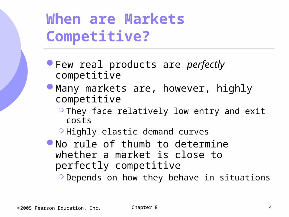
Few real products are perfectly competitive
Many markets are, however, highly competitive They face relatively low entry and exit costs Highly elastic demand curves
No rule of thumb to determine whether a market is close to perfectly competitive Depends on how they behave in situations

Chapter 8 5©2005 Pearson Education, Inc.
Profit Maximization
Do firms maximize profits? Managers in firms may be concerned with
other objectivesRevenue maximizationRevenue growthDividend maximizationShort-run profit maximization (due to bonus or
promotion incentive) Could be at expense of long run profits

Chapter 8 6©2005 Pearson Education, Inc.
Profit Maximization
Implications of non-profit objective Over the long run, investors would not
support the company Without profits, survival is unlikely in
competitive industries
Managers have constrained freedom to pursue goals other than long-run profit maximization

Chapter 8 7©2005 Pearson Education, Inc.
Marginal Revenue, Marginal Cost, and Profit Maximization
We can study profit maximizing output for any firm, whether perfectly competitive or not Profit () = Total Revenue - Total Cost If q is output of the firm, then total revenue is
price of the good times quantity Total Revenue (R) = Pq

Chapter 8 8©2005 Pearson Education, Inc.
Marginal Revenue, Marginal Cost, and Profit Maximization
Costs of production depends on output Total Cost (C) = C(q)
Profit for the firm, , is difference between revenue and costs
)()()( qCqRq
Chapter 8 9©2005 Pearson Education, Inc.
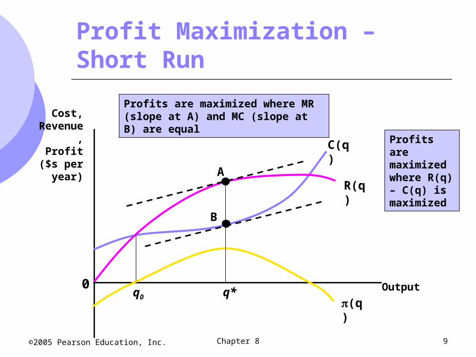
Profit Maximization – Short Run
0
Cost,Revenue,
Profit($s per
year)
Output
C(q)
R(q)A
B
(q)q0 q*
Profits are maximized where MR (slope at A) and MC (slope at B) are equal
Profits are maximized where R(q) – C(q) is maximized

Chapter 8 10©2005 Pearson Education, Inc.
Marginal Revenue, Marginal Cost, and Profit Maximization
Profit is maximized at the point at which an additional increment to output leaves profit unchanged
MCMR
MCMR
q
C
q
R
q
CR
0
0

Chapter 8 11©2005 Pearson Education, Inc.
Marginal Revenue, Marginal Cost, and Profit Maximization
The Competitive Firm Price taker – market price and output
determined from total market demand and supply
Market output (Q) and firm output (q) Market demand (D) and firm demand (d)

Chapter 8 12©2005 Pearson Education, Inc.
The Competitive Firm
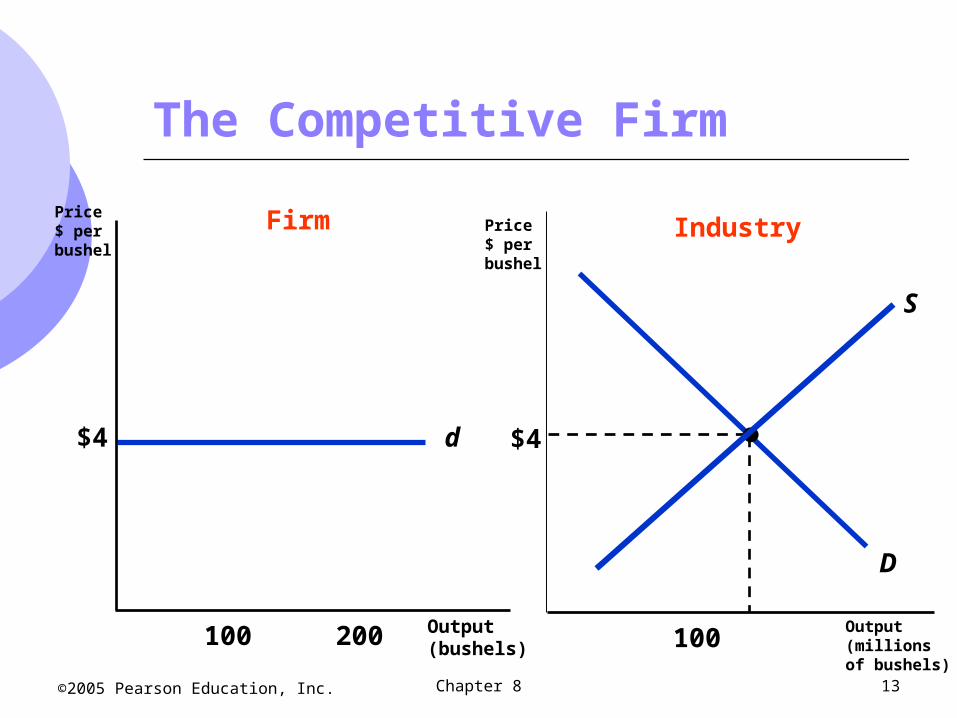
Demand curve faced by an individual firm is a horizontal line Firm’s sales have no effect on market price
Demand curve faced by whole market is downward sloping Shows amount of goods all consumers will
purchase at different prices
Chapter 8 13©2005 Pearson Education, Inc.
The Competitive Firm
d$4
Output (bushels)
Price$ per bushel
100 200
Firm Industry
D
$4
S
Price$ per bushel
Output (millions of bushels)
100

Chapter 8 14©2005 Pearson Education, Inc.
The Competitive Firm
The competitive firm’s demand Individual producer sells all units for $4
regardless of that producer’s level of output MR = P with the horizontal demand curve For a perfectly competitive firm, profit
maximizing output occurs when
ARPMRqMC )(

Chapter 8 15©2005 Pearson Education, Inc.
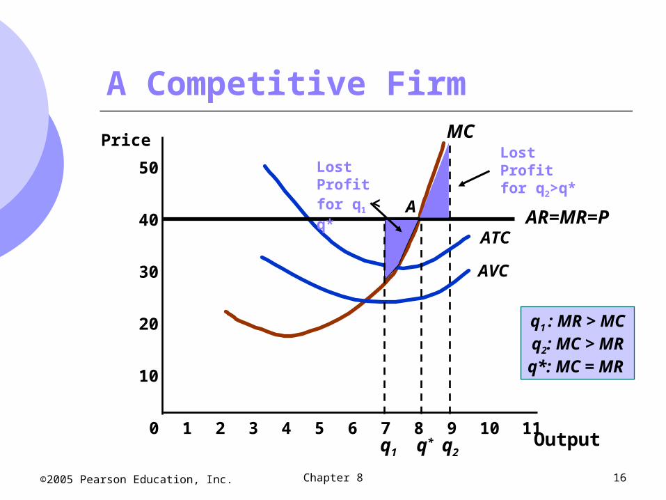
Choosing Output: Short Run
In the short run, capital is fixed and firm must choose levels of variable inputs to maximize profits
We can look at the graph of MR, MC, ATC and AVC to determine profits
The point where MR = MC, the profit maximizing output is chosen
Chapter 8 16©2005 Pearson Education, Inc.
q2
A Competitive Firm
10
20
30
40
Price
50
MC
AVC
ATC
0 1 2 3 4 5 6 7 8 9 10 11Outputq*
AR=MR=PA
q1 : MR > MCq2: MC > MRq*: MC = MR
q1
Lost Profit for q2>q*Lost Profit
for q1 < q*

Chapter 8 17©2005 Pearson Education, Inc.
A Competitive Firm – Positive Profits
10
20
30
40
Price
50
0 1 2 3 4 5 6 7 8 9 10 11Outputq2
MC
AVC
ATC
q*
AR=MR=PA
q1
D
C B Profits are determined
by output per unit times quantity
Profit per unit = P-AC(q) = A to B
Total Profit = ABCD

Chapter 8 18©2005 Pearson Education, Inc.
The Competitive Firm
A firm does not have to make profitsIt is possible a firm will incur losses if the
P < AC for the profit maximizing quantity Still measured by profit per unit times
quantity Profit per unit is negative (P – AC < 0)

Chapter 8 19©2005 Pearson Education, Inc.
A Competitive Firm – Losses
Price
Output
MC
AVC
ATC
P = MRD
At q*: MR = MC and P < ATCLosses = (P- AC) x q* or ABCD
q*
A
BC

Chapter 8 20©2005 Pearson Education, Inc.
Choosing Output in the Short Run
Summary of Production Decisions Profit is maximized when MC = MR If P > ATC the firm is making profits If P < ATC the firm is making losses

Chapter 8 21©2005 Pearson Education, Inc.
Short Run Production
Why would a firm produce at a loss? Might think price will increase in near future Shutting down and starting up could be
costly
Firm has two choices in short run Continue producing Shut down temporarily Will compare profitability of both choices

Chapter 8 22©2005 Pearson Education, Inc.
Short Run Production
When should the firm shut down? If AVC < P < ATC, the firm should continue
producing in the short runCan cover all of its variable costs and some of
its fixed costs If AVC > P < ATC, the firm should shut down
Cannot cover its variable costs or any of its fixed costs

Chapter 8 23©2005 Pearson Education, Inc.
A Competitive Firm – Losses
Price
Output
P < ATC but AVC so firm will continue to produce in short run
MC
AVC
ATC
P = MRD
q*
A
BC
Losses
EF

Chapter 8 24©2005 Pearson Education, Inc.
Competitive Firm – Short Run Supply
Supply curve tells how much output will be produced at different prices
Competitive firms determine quantity to produce where P = MC Firm shuts down when P < AVC
Competitive firms’ supply curve is portion of the marginal cost curve above the AVC curve

Chapter 8 25©2005 Pearson Education, Inc.
A Competitive Firm’sShort-Run Supply Curve
Price($ per
unit)
Output
MC
AVC
ATC
P = AVC
P2
q2
The firm chooses theoutput level where P = MR = MC,
as long as P > AVC.
P1
q1
S
Supply is MC above AVC

Chapter 8 26©2005 Pearson Education, Inc.
MC2
q2
Input cost increases and MC shifts to MC2
and q falls to q2.
MC1
q1
The Response of a Firm toa Change in Input Price
Price($ per
unit)
Output
$5
Savings to the firmfrom reducing output

Chapter 8 27©2005 Pearson Education, Inc.
Short-Run Market Supply Curve
Shows the amount of product the whole market will produce at given prices
Is the sum of all the individual producers in the market
We can show graphically how we can sum the supply curves of individual producers

Chapter 8 28©2005 Pearson Education, Inc.
MC3
Industry Supply in the Short Run$ perunit
MC1
SSThe short-runindustry supply curve
is the horizontalsummation of the supply
curves of the firms.
Q
MC2
15 21
P1
P3
P2
1082 4 75

Chapter 8 29©2005 Pearson Education, Inc.
Long-Run Competitive Equilibrium
For long run equilibrium, firms must have no desire to enter or leave the industry
Relate economic profit to the incentive to enter and exit the market
Relate accounting profit to economic profit

Chapter 8 30©2005 Pearson Education, Inc.
Long-Run Competitive Equilibrium
Accounting profit Difference between firm’s revenues and
direct costs
Economic profit Difference between firm’s revenues and
direct and indirect costs Takes into account opportunity costs

Chapter 8 31©2005 Pearson Education, Inc.
Long-Run Competitive Equilibrium
Firm uses labor (L) and capital (K) with purchased capital
Accounting Profit and Economic Profit Accounting profit: = R - wL Economic profit: = R = wL - rK
wl = labor costrk = opportunity cost of capital

Chapter 8 32©2005 Pearson Education, Inc.
Long-Run Competitive Equilibrium
Zero-Profit A firm is earning a normal return on its
investment Doing as well as it could by investing its
money elsewhere Normal return is firm’s opportunity cost of
using money to buy capital instead of investing elsewhere
Competitive market long run equilibrium

Chapter 8 33©2005 Pearson Education, Inc.
Long-Run Competitive Equilibrium
Zero Economic Profits If R > wL + rk, economic profits are positive If R = wL + rk, zero economic profits, but the
firm is earning a normal rate of return, indicating the industry is competitive
If R < wl + rk, consider going out of business
Chapter 8 34©2005 Pearson Education, Inc.
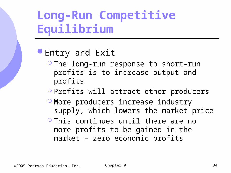
Long-Run Competitive Equilibrium
Entry and Exit The long-run response to short-run profits is
to increase output and profits Profits will attract other producers More producers increase industry supply,
which lowers the market price This continues until there are no more profits
to be gained in the market – zero economic profits

Chapter 8 35©2005 Pearson Education, Inc.
Long-Run Competitive Equilibrium – Profits
S1
Output Output
$ per unit ofoutput
$ per unit ofoutput
LAC
LMC
D
S2
$40 P1
Q1
Firm Industry
Q2
P2
q2
$30
•Profit attracts firms•Supply increases until profit = 0

Chapter 8 36©2005 Pearson Education, Inc.
Long-Run Competitive Equilibrium – Losses
S2
Output Output
$ per unit ofoutput
$ per unit ofoutput
LAC
LMC
D
S1
P2
Q2
Firm Industry
Q1
P1
q2
$20
$30
•Losses cause firms to leave•Supply decreases until profit = 0

Chapter 8 37©2005 Pearson Education, Inc.
Long-Run Competitive Equilibrium
1. All firms in industry are maximizing profits
MR = MC
2. No firm has incentive to enter or exit industry
Earning zero economic profits
3. Market is in equilibrium QD = QS

Chapter 8 38©2005 Pearson Education, Inc.
Choosing Output in the Long Run
Economic Rent The difference between what firms are willing
to pay for an input less the minimum amount necessary to obtain it
When some have accounting profits that are larger than others, they still earn zero economic profits because of the willingness of other firms to use the factors of production that are in limited supply

Chapter 8 39©2005 Pearson Education, Inc.
Choosing Output in the Long Run
An Example Two firms A & B that both own their land A is located on a river which lowers A’s
shipping cost by $10,000 compared to B The demand for A’s river location will
increase the price of A’s land to $10,000 = economic rent
Although economic rent has increased, economic profit has become zero

Chapter 8 40©2005 Pearson Education, Inc.
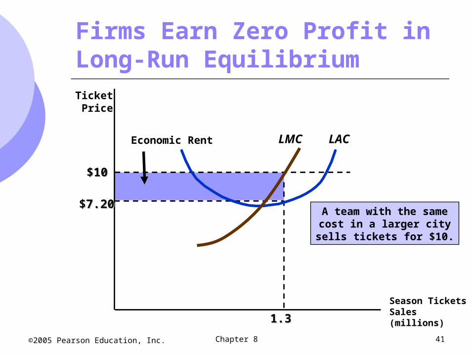
Firms Earn Zero Profit inLong-Run EquilibriumTicketPrice
Season TicketsSales (millions)
$7$7
1.01.0
A baseball teamin a moderate-sized city
sells enough tickets so that price is equal to marginal
and average cost(profit = 0).
LACLMC
Chapter 8 41©2005 Pearson Education, Inc.
1.31.3
$10$10
Economic Rent
TicketPrice
$7.20$7.20A team with the samecost in a larger citysells tickets for $10.
Firms Earn Zero Profit inLong-Run Equilibrium
Season TicketsSales (millions)
LACLMC
Chapter 8 42©2005 Pearson Education, Inc.
Firms Earn Zero Profit inLong-Run Equilibrium
With a fixed input such as a unique location, the difference between the cost of production (LAC = 7) and price ($10) is the value or opportunity cost of the input (location) and represents the economic rent from the input

Chapter 8 43©2005 Pearson Education, Inc.
Firms Earn Zero Profit inLong-Run Equilibrium
If the opportunity cost of the input (rent) is not taken into consideration, it may appear that economic profits exist in the long run (positive accounting profits)