2009:062 civ master's thesis
TRANSCRIPT

2009:062 CIV
M A S T E R ' S T H E S I S
Analysis of an Engine FrameSubjected to Large Imbalance Loads
Niklas Blind Rickard Östlund
Luleå University of Technology
MSc Programmes in Engineering Mechanical Engineering
Department of Applied Physics and Mechanical EngineeringDivision of Solid Mechanics
2009:062 CIV - ISSN: 1402-1617 - ISRN: LTU-EX--09/062--SE


Abstract
This master thesis deals with the load carrying capability of a turbine exhaustcase subjected to large imbalance loads. The event is transient dynamic toits nature and displays non-linear features such as plasticity and large deflec-tions. The main result sought is the ultimate load to which structural integritycan be guaranteed. Results are compared between dynamic and quasi-staticanalyses and the methods are evaluated. The ability to overcome computa-tional difficulties and the solver time are compared between three finite ele-ment solvers. Abaqus/Explicit is compared to LS-DYNA in dynamic analysisand Abaqus/Standard is compared to ANSYS in quasi-static analysis. Theresults show consistency between analysis methods and solvers. LS-DYNA isfaster than Abaqus/Explicit and Abaqus/Standard is faster than ANSYS forthe simulations performed in this thesis.


Sammanfattning
I examensarbetet undersoks analysmetoder for dimensionering av ett bakre tur-binstativ utsatt for stora obalanslaster. Forloppet ar transient och ickelinjartda plasticitet och stora deformationer ingar i responsen. Maximal lastbarandeformaga av det bakre turbinstativet ar det huvudsakliga resultatet som soks.Resultat fran dynamisk och kvasi-statisk analys jamfors och analysmetodernautvarderas. Tre kommersiella finita element losare anvands for att underso-ka hur berakningstekniska svarigheter hanteras, och hur resultat och berak-ningstid forhaller sig mellan losarna. Abaqus/Explicit och LS-DYNA jamforsi dynamisk analys och Abaqus/Standard och ANSYS jamfors i kvasi-statiskanalys. Resultaten visar pa god overensstammelse mellan analysmetoder ochmellan losare. Det visar sig att LS-DYNA ar snabbare an Abaqus/Explicit ochatt Abaqus/Standard ar snabbare an ANSYS for analyserna utforda i dettaexamensarbete.


Preface
This master thesis is the final project for the Master of Science programme inMechanical Engineering at Lulea University of Technology. The master thesiswas performed at Volvo Areo Corporation in Trollhattan at the department ofsolid mechanics and structural dynamics.
We would like to thank our supervisors Ph.D John Eriksson and Ph.DRobert Tano for their support and commitment and for making this projectpossible. We send our gratitude to the people at the department of solid me-chanics and structural dynamics for providing a stimulating environment.
We would also like to thank for the software support from Mr. JoakimAsklund, Mr. Ulf Karlsson and Mr. Jan Rydin at Simulia Scandinavia AB,Ph.D Daniel Hilding at Engineering Research Nordic AB and Mr. Mikael Lauthat Medeso AB.
Finally we thank our examiner at the university, Prof. Mats Oldenburg forsupporting our work.
Your contribution is greatly appreciated.
Niklas Blind and Rickard Ostlund
Trollhattan, March 2009
5

6

Contents
1 Introduction 151.1 Aim and scope . . . . . . . . . . . . . . . . . . . . . . . . . . . 151.2 Turbo fan jet engine . . . . . . . . . . . . . . . . . . . . . . . . 151.3 Volvo Aero Corporation . . . . . . . . . . . . . . . . . . . . . . 151.4 Turbine exhaust case . . . . . . . . . . . . . . . . . . . . . . . . 161.5 Design requirements . . . . . . . . . . . . . . . . . . . . . . . . 171.6 Fan blade out . . . . . . . . . . . . . . . . . . . . . . . . . . . . 171.7 Structural collapse . . . . . . . . . . . . . . . . . . . . . . . . . 18
2 Theory 212.1 Governing equations . . . . . . . . . . . . . . . . . . . . . . . . 212.2 Large deformation . . . . . . . . . . . . . . . . . . . . . . . . . 222.3 Elastoplasticity . . . . . . . . . . . . . . . . . . . . . . . . . . . 232.4 Solution procedures . . . . . . . . . . . . . . . . . . . . . . . . 25
2.4.1 Explicit dynamic analysis . . . . . . . . . . . . . . . . . 252.4.2 Quasi-static analysis . . . . . . . . . . . . . . . . . . . . 262.4.3 Implicit dynamic analysis . . . . . . . . . . . . . . . . . 272.4.4 Linear buckling analysis . . . . . . . . . . . . . . . . . . 28
3 Method 313.1 Finite element model . . . . . . . . . . . . . . . . . . . . . . . . 313.2 Material . . . . . . . . . . . . . . . . . . . . . . . . . . . . . . . 323.3 Boundary conditions . . . . . . . . . . . . . . . . . . . . . . . . 323.4 Elements . . . . . . . . . . . . . . . . . . . . . . . . . . . . . . 343.5 Explicit dynamic solution method . . . . . . . . . . . . . . . . 353.6 Quasi-static solution method . . . . . . . . . . . . . . . . . . . 363.7 Implicit dynamic solution method . . . . . . . . . . . . . . . . 39
4 Results 414.1 Failure mode . . . . . . . . . . . . . . . . . . . . . . . . . . . . 414.2 Explicit dynamic . . . . . . . . . . . . . . . . . . . . . . . . . . 424.3 Quasi-static . . . . . . . . . . . . . . . . . . . . . . . . . . . . . 454.4 Implicit dynamic . . . . . . . . . . . . . . . . . . . . . . . . . . 48
7

5 Conclusions 515.1 Method and accuracy . . . . . . . . . . . . . . . . . . . . . . . 515.2 Simulation time . . . . . . . . . . . . . . . . . . . . . . . . . . . 51
6 Further work 53
A Appendix figures. Explicit dynamic 55
B Appendix figures. Quasi-static 63
C Appendix figures. Implicit dynamic 67
D Appendix. Analysis equipment 69
Bibliography 71
8

List of Figures
1.1 Engine Alliance GP7000 turbo fan jet engine [1]. . . . . . . . . 161.2 Turbine Exhaust Case. . . . . . . . . . . . . . . . . . . . . . . . 161.3 Schematic cross-section of a typical turbo fan jet engine. . . . . 171.4 Snap-through buckling. . . . . . . . . . . . . . . . . . . . . . . 181.5 Bifurcation buckling. . . . . . . . . . . . . . . . . . . . . . . . . 19
2.1 Elastic response left and elasto-plastic response right. . . . . . 242.2 Von Mises yield surface in the principal stress space. . . . . . . 242.3 A schematic load deflection curve showing a local instability point. 27
3.1 Exploded view of the FE-model. . . . . . . . . . . . . . . . . . 313.2 Crossection view of applied loads and constraints. . . . . . . . . 323.3 Axial view of applied loads. . . . . . . . . . . . . . . . . . . . . 333.4 Typical FBO force transients. . . . . . . . . . . . . . . . . . . . 333.5 Output of specific node displacements and cross section forces. 36
4.1 Failure mode. . . . . . . . . . . . . . . . . . . . . . . . . . . . . 414.2 Strut sub-model of TEC. . . . . . . . . . . . . . . . . . . . . . . 434.3 Element stiffness comparison using the sub-model. . . . . . . . 434.4 CPU scaling comparison, for explicit solvers using Model 1. . . 454.5 Failure mode results from Abaqus. Quasi-static left and explicit
dynamic right. . . . . . . . . . . . . . . . . . . . . . . . . . . . 464.6 A typical local buckle, rendering in a too early simulation abortion. 474.7 Time incrementation comparison ANSYS blue and Abaqus/Standard
black. . . . . . . . . . . . . . . . . . . . . . . . . . . . . . . . . 47
A.1 von Mises stress Model 1, aft looking forward. LS-DYNA leftand Abaqus/Explicit right. . . . . . . . . . . . . . . . . . . . . 55
A.2 von Mises stress Model 1, forward looking aft. LS-DYNA leftand Abaqus/Explicit right. . . . . . . . . . . . . . . . . . . . . 56
A.3 Plastic strain Model 1, aft looking forward. LS-DYNA left andAbaqus/Explicit right. . . . . . . . . . . . . . . . . . . . . . . . 56
A.4 Plastic strain Model 1, forward looking aft. LS-DYNA left andAbaqus/Explicit right. . . . . . . . . . . . . . . . . . . . . . . . 57
9
A.5 von Mises stress Model 2, aft looking forward. LS-DYNA leftand Abaqus/Explicit right. . . . . . . . . . . . . . . . . . . . . 57
A.6 von Mises stress Model 2, forward looking aft. LS-DYNA leftand Abaqus/Explicit right. . . . . . . . . . . . . . . . . . . . . 58
A.7 Plastic strain Model 2, aft looking forward. LS-DYNA left andAbaqus/Explicit right. . . . . . . . . . . . . . . . . . . . . . . . 58
A.8 Plastic strain Model 2, forward looking aft. LS-DYNA left andAbaqus/Explicit right. . . . . . . . . . . . . . . . . . . . . . . . 59
A.9 Resultant displacement for mount lugs and bearing, Model 1. . 59A.10 External work, 125% load factor, Model 1. . . . . . . . . . . . . 60A.11 Resultant section forces, Model 1. . . . . . . . . . . . . . . . . . 60A.12 External work, 119% load factor, Model 1. . . . . . . . . . . . . 61A.13 External work. LS-DYNA only shell type 16. Abaqus/Explicit
Model 1. . . . . . . . . . . . . . . . . . . . . . . . . . . . . . . . 61A.14 Sub-model reaction forces for different hourglass formulation.
Red is viscous and blue is stiffness based. . . . . . . . . . . . . 61A.15 Sub-model reaction force for different shell types. . . . . . . . . 62
B.1 von Mises stress. Explicit dynamic method left and quasi-staticmethod right. . . . . . . . . . . . . . . . . . . . . . . . . . . . . 63
B.2 Plastic strain. Explicit dynamic method left and quasi-staticmethod right. . . . . . . . . . . . . . . . . . . . . . . . . . . . . 64
B.3 Displacement, 3 times magnified. ANSYS left and Abaqus/Standardright. . . . . . . . . . . . . . . . . . . . . . . . . . . . . . . . . . 64
B.4 von Mises stress. ANSYS left and Abaqus/Standard right. . . . 65B.5 Displacement of left mount lug. ANSYS blue and Abaqus/Standard
black. . . . . . . . . . . . . . . . . . . . . . . . . . . . . . . . . 65B.6 Dissipated stabilization energy. ANSYS blue and Abaqus/Standard
black. . . . . . . . . . . . . . . . . . . . . . . . . . . . . . . . . 66
C.1 von Mises stress dynamic analysis. Explicit left and implicit right. 67
10

List of Tables
3.1 Element types used in explicit dynamic simulations. . . . . . . 343.2 Element types used in quasi-static and implicit dynamic simula-
tions. . . . . . . . . . . . . . . . . . . . . . . . . . . . . . . . . . 353.3 Load stepping. . . . . . . . . . . . . . . . . . . . . . . . . . . . 373.4 Time control, quasi-static. . . . . . . . . . . . . . . . . . . . . . 38
4.1 Shell element integration. . . . . . . . . . . . . . . . . . . . . . 424.2 Minimum loadfactor triggering collapse. . . . . . . . . . . . . . 444.3 Model 1 time comparison, explicit dynamic. . . . . . . . . . . . 444.4 Model 2 time comparison, explicit dynamic. . . . . . . . . . . . 444.5 Quasi-static solution, time comparison to global collapse. . . . 484.6 Quasi-static solution, time comparison to 100% load. . . . . . . 484.7 Simulation time, dynamic implicit. . . . . . . . . . . . . . . . . 49
11

12

Nomenclature
Tensorial quantities
σij Cauchy stressfi Body loadui Displacementui Velocityui Accelerationni Surface normalti Surface tractionδvi virtual velocityεij Total strainεeij Elastic strainεpij Plastic strainδij Dirac delta function,αij Back stressC Elastic constitutive tangentD Rate of deformationΩ Spin
Vector and matrix quantities
x Spatial coordinate of material pointu Nodal displacementu Nodal velocitiesu Nodal accelerationsNn Displacement interpolation functionM Mass matrixF Deformation gradientFext External forcesFint Internal forcesFv Viscous damping forcesσ Cauchy stressK Material stiffnessKσ Stress stiffness
13

Scalar quantities
ρ Mass densityt Timeσy0 Initial yield stressσy Yield stressc Damping constantλ Load factorωf Load frequencyω0 Fundamental frequency
14

Chapter 1
Introduction
1.1 Aim and scope
In this master thesis methods for ultimate strength analysis of a Turbine Ex-haust Case (TEC) are reviewed. The purpose is to contribute to Volvo Aeromethod development by evaluation of solution methods and commercial finiteelement solvers. The studied event is transient dynamic and requires non-linearanalysis. A dynamic and a quasi-static method are used to investigate eachmethods appropriateness and efficiency. Abaqus/Explicit and LS-DYNA arecompared in a transient dynamic analysis and ANSYS and Abaqus/Standardare compared in a quasi-static analysis. The solver efficiency is evaluated interms of analysis time. As an alternative method a dynamic approach usingimplicit time integration is studied briefly.
1.2 Turbo fan jet engine
The Engine Alliance GP7000, figure 1.1, is a turbo fan jet engine developed bya joint venture between GE Aircraft Engines and Pratt & Whitney. With 363kN of thrust this engine powers the Airbus super-jumbo A380. The GP7000 is atwo-spool architecture high-bypass ratio turbo fan engine with 2.95 m diameterfan and a dry weight of 6712 kg.
1.3 Volvo Aero Corporation
Volvo Aero develops and manufactures components for commercial and militaryaircraft engines, rocket engines and gas turbine derivatives for power- and heatgeneration. Volvo Aero is specialized in light-weight technology which hasrendered to a development and manufacturing contract for the component inquestion, a Turbine Exhaust Case (TEC).
15

Figure 1.1: Engine Alliance GP7000 turbo fan jet engine [1].
1.4 Turbine exhaust case
The TEC, figure 1.2, is located between the Low Pressure Turbine (LPT) andthe exhaust components. The TEC studied in this master thesis consist of a
Figure 1.2: Turbine Exhaust Case.
hub which attaches to the bearing housing and 13 struts welded between thehub and the outer case. The aerofoil shaped struts serve as a load transferbetween the bearing and engine mount. Three mount lugs are situated at thetop which attaches the aft section of the engine to the aircraft wing pylon. Themost important functions the TEC provides are:
- Low Pressure Turbine discharge flow path and reduce swirl to obtainstraight axial thrust.
- Load transfer between bearing and engine mount.
All the major parts in a turbo fan engine are shown in figure 1.3. Fromthe left, the Fan, Low Pressure Compressor (LPC), High Pressure Compressor(HPC), High Pressure Turbine (HPT), Low Pressure Turbine (LPT) and finallythe Turbine Exhaust Case (TEC).
16

Figure 1.3: Schematic cross-section of a typical turbo fan jet engine.
1.5 Design requirements
To ensure the functionality, several design requirements are imposed on theTEC. A simplified form of the structural requirements is listed below followedby a short description:
- Ultimate strength: Ultimate loads must be sustained without separationfrom the aircraft, i.e. load path must remain intact. For ultimate loadssee section 1.6.
- Limit strength: Loads expected to occur once per 50 000 flight hours mustbe sustained without detrimental permanent deformation, which wouldinterfere with safe engine operation.
- Life requirements: TEC must be designed to function through out itsdeclared flight envelope. Total life must exceed service life and componentresonances must be placed outside engine operating speed.
- Stiffness: TEC must provide acceptable engine stability and prevent rotorblade closure during flight manoeuvres.
1.6 Fan blade out
There are different ultimate loads such as wheel upp landing, fan blade out,bird ingestion etc. This thesis is restricted to the Fan Blade Out (FBO) event.In order to ensure safety, a turbo fan jet engine must be designed to withstandthe loss of a fan blade rotating at high speed. This event is also known as afan blade out and is one of the most violent loading conditions a TEC can besubjected to. The resulting rotor imbalance generates large forces on the entireengine carcass. As mentioned earlier the TEC design must accommodate theseloads with integrity of engine and part.
17

1.7 Structural collapse
Due to the slender design of struts of the TEC, the predominant failure modeduring ultimate load conditions is a sudden loss of structural integrity, owingto a combination of material failure and buckling. It is therefore important todetermine the margin to collapse, and evaluate whether material failure occursbelow this margin. There are several methods to determine margin to collapseof structures:
- Handbook solutions
- Linear buckling analysis, i.e. eigenvalue analysis
- Non-linear quasi-static analysis
- Non-linear dynamic analysis
This thesis deals with the two latter approaches.The term collapse often refers to sudden loss of structural integrity and does
not distinguish between the two major categories leading to failure: materialfailure or structural instability due to loss of stiffness within elastic limit. Theterm buckling is often reserved specifically for the latter category. Materialfailure and buckling may occur in sequence, leading to structural collapse, e.g.localized plastic behaviour which lowers the stiffness, leading to buckling.
When considering the response of a structure undergoing buckling as equi-librium between load and displacement, and the path of this equilibrium istraced as the load is increased, the response can either follow a single equilib-rium path or shift between paths. The first is called snap-trough behaviour and
Figure 1.4: Snap-through buckling.
can be illustrated by a curved beam with concentrated point load, figure 1.4.The displacements of the new configuration are predominantly in the samedirection as the applied loading. The second is called bifurcation buckling,and can be characterized by an idealized axially loaded column. A bifurcationpoint is the intersection of two equilibrium paths, i.e. there is two displacement
18

Figure 1.5: Bifurcation buckling.
solutions for the same load increment, figure 1.5. Above this point the struc-ture will shift from one displacement mode to another, with secondary pathdisplacements orthogonal to load direction.
The analysis main output is collapse load factor, i.e. at which multiple ofthe applied load the structural integrity cannot be guaranteed.
19

20
Chapter 2
Theory
2.1 Governing equations
Newton’s second law of motion states that the net force on a particle is propor-tional to the time rate of change of its linear momentum. We seek a solutionto this momentum equation
σij,j + fi = ρui , (2.1)
that satisfies the traction boundary conditions σijni = ti(t) and the displace-ment boundary conditions ui = Di(t).
The weak form of (2.1) may be obtained trough the principle of virtualwork, by multiplying the differential equations by an arbitrary, vector-valuedtest function, over the entire volume, and integrating. The test function can bea velocity field, δv, which is completely arbitrary except that it must obey anyprescribed kinematical constraints and have sufficient continuity. The productof this test function with the equilibrium force field then represents the virtualwork rate
δπ =∫V
ρuiδvidV +∫V
σijδvi,jdV −∫V
fiδvidV −∫S
tiδvidS = 0 . (2.2)
The virtual work statement has a simple physical interpretation: the rate ofwork done by the external forces subjected to any virtual velocity field is equalto the rate of work done by the equilibrating stresses on the rate of deformationof the same virtual velocity field.
The basis for the development of a displacement-interpolation finite elementmodel is the introduction of some locally based spatial approximation to partsof the solution. The finite element displacement interpolator can be written ingeneral as
u = Nnun . (2.3)
21

WhereNn are interpolation functions that depend on some material coordinatesystem and un are nodal displacements.
Since δv must be compatible with all kinematical constraints, it must havethe same spatial variation as the assumed displacements
δv = Nnδvn . (2.4)
The second integral term in (2.2), the internal virtual work, is rewritten in termsof any work conjugate pair of stress and strain, and the continuum variationstatement (2.2) is approximated over the finite set δvn ,
δvn(∫
V
ρNTNdV u+∫V
BTσdV −∫V
NTfdV −∫S
NT tdS
)= 0 . (2.5)
We can choose each δvn to be non-zero and all others zero in turn, to arrive ata system of non-linear equations∫
V
ρNTNdV u+∫V
BTσdV −∫V
NTfdV −∫S
NT tdS = 0 . (2.6)
The matrix B that defines the strain variation from the variations of the kine-matical variables is derivable immediately from the interpolation functions Nonce the particular strain measure to be used is defined. This system forms thebasis for the standard assumed displacement finite element analysis procedurewhere
M =∫V
ρNTNdV , (2.7)
F int =∫V
BTσdV , (2.8)
F ext =∫V
NTfdV +∫S
NT tdS . (2.9)
Arriving at the equation of motion
Mu+ F int(u) = F ext . (2.10)
This equation system is then solved for u in time, which are described in section2.4.
2.2 Large deformation
When geometrical changes have a significant effect on the load deflection char-acteristics of the structure, a linear response assumption is no longer valid. Forthis non-linear buckling analysis an updated Lagrangian formulation is used.All integrals of equation (2.9) are calculated with respect to a known deformed
22

configuration and are continually updated as the calculation proceeds, i.e. anincremental solution.
In a material or Lagrangian formulation the position of a particle is givenin terms of the previous position of that same particle
x = x(X, t) , (2.11)
and the velocity of the particle is
v = x(X, t) . (2.12)
Since the discrete equilibrium is formulated in current deformed configurationthe stress measure used is the Cauchy stress. The strain rate measure, whichis work conjugate to Cauchy stress, is the rate of deformation, D. The rate ofdeformation is defined as
D =12
(L+LT ) (2.13)
Where L = ( ∂v∂x ). During rigid body motion, D is unchanged meaning thatno material straining occurs. To account for changes in geometry the Cauchystress must be updated objectively to rigid body rotations. There are severalmethods for this, where the most common for hypo-elastoplastic approach isthe Truesdell, Green-Naghdi and Jaumann rates. The Jaumann rate of Cauchystress is defined
σ = C ·D + Ω · σ − σ ·Ω , (2.14)
WhereC is the constitutive matrix, and Ω is the spin defined as Ω = 12 (L−LT ).
Stress is then updated σt+∆t = σt + ∆t · σ. Thus the internal forces arecomputed with respect to deformed configuration and with a stress measurethat accounts for changes in configuration.
For a thurough description on large deformation and its measures see [2].
2.3 Elastoplasticity
Constitutive equations describe the materials deformation properties as a re-lation between stress and strain. When the relation is a linear function thematerial is elastic, which is the simplest material model. For isotropic materi-als this relation is expressed by Hooke’s law
σij = 3K(
13εkkδij
)+ 2G
(εij −
13εkkδij
). (2.15)
Where the first term is the hydrostatic pressure component and the second isthe deviatoric stress tensor. K is the compression modulus and G is the shearmodulus. This constitutive relation is only valid for linear response. In the caseof elasto-plastic response the total strain can be given by the sum of elastic andplastic strain
εij = εeij + εpij . (2.16)
23

Figure 2.1: Elastic response left and elasto-plastic response right.
The elastic strain is recovered when the material is unloaded, which is not thecase for the plastic strain, see figure 2.1. At σy0 the material starts to yield,and to capture this non-linear behaviour a hardening law needs to be applied.A systematic treatment of constitutive relations is often done by defining ayield surface
f(σij − αij , σy(κ)
)= 0 , (2.17)
shown in figure 2.2, where
Figure 2.2: Von Mises yield surface in the principal stress space.
σy(κ) = σy0 + σy(εp) , (2.18)
and κ is the hardening parameter. For strain proportional hardening κ = εp.If f < 0 strain state is elastic, f > 0 is non-physical. There are several
measures to find yield stress, and here the associative von Mises flow rule isused. For isotropic hardening material without Baushinger effect (αij = 0) theyield function is defined as
f(σij , σy(κ)
)=(
32sijsji
) 12
− σy(κ) . (2.19)
Where sij is the deviatoric stress tensor, which is defined as the stress tensorminus the hydrostatic pressure tensor
sij = σij −13σkkδij . (2.20)
With an isotropic hardening rule the yield surface expands radially in the prin-cipal stress space when the material yields, as opposed by a kinematical hard-ening law where the yield surface translates.
24

The relation between the yield stress σy and the effective plastic strain εp
is obtained from a material uni-axial test specimen and is used as input datadefining the plastic response of the materials used in the model.
These three components, yield criterion, flow rule and hardening law arethe fundamental components of incremental plasticity theory. For detailedtreatment of this topic see [3].
2.4 Solution procedures
The equilibrium equations (2.10) can be solved by direct integration. Either aquasi-static approach can be used, when inertia forces are considered insignifi-cant, or a fully dynamic. Both require the use of incremental solution schemes,as the structures response is non-linear. Solution is obtained by integratingthe equations of motion with respect to time, either physical time or some ar-tificial time. The artificial time scale refers to the quasi-static solution whenvelocities and accelerations are zero. In order to solve the dynamic equation,an assumption is made regarding how the acceleration varies over a small timeinterval ∆t. Available dynamic integration schemes are broadly characterizedas explicit or implicit. For the quasi-static approach the non-linear equilibriumequation is linearised with a 1st order Taylor expansion in time, and then solvedincrementally with the Newton-Rhapson method.
2.4.1 Explicit dynamic analysis
For explicit time integration the central difference operator is used
u =ut+∆t − ut−∆t
2∆t, u =
ut+∆t − 2ut + ut−∆t
∆t2, (2.21)
these approximations in the equilibrium equation 2.10 yields
M
(ut+∆t − 2ut + ut−∆t
∆t2
)+ F int(u)t = F text , (2.22)
with rearranged terms
ut+∆t = 2ut − ut−∆t + ∆t2M−1(F text − Ftint) . (2.23)
When the time step is small the stiffness term F int(u) will not change signif-icantly over the step, hence no iteration is needed to find equilibrium. Usinga lumped mass matrix, i.e. all mass terms are added row wise to the maindiagonal. This uncouples the equation system such that the equations can besolved on element-by-element basis; hence no need to form global stiffness norelement stiffness matrix. Inversion of M is trivial since the matrix is diagonal.
25

The explicit integration operator is conditionally stable, and the largeststable time increment, ∆t, depends on the characteristic element length, Le,the material stiffness, E, and the density, ρ, as follows
∆t ≤ Le√Eρ
. (2.24)
2.4.2 Quasi-static analysis
The quasi-static solution procedure assumes that acceleration and velocitiesare zero, reducing the equilibrium equation to
F int(u)− F ext = 0 . (2.25)
Since the equation is non-linear it must be solved by incrementally stepping upthe external force, F ext, and updating the displacements, u. Equation (2.25)is reformulated to a residual problem
R(u) = F int(u)− F ext . (2.26)
Every force increment the displacements are updated iteratively until the resid-ual criteria is reached.
In the following presentation subscript denotes iteration number and su-perscript denotes increment number, and the unknown ut+∆t is solved from aknown state ut. The right hand side of equation (2.26) is expanded in a Taylorseries about the sought variable ut+∆t,
R(ut+∆ti ) = F int(ut+∆t
i ) +Ktan(ut+∆ti )(ut+∆t
i+1 − ut+∆ti )− F t+∆t
ext , (2.27)
Ktan(ut+∆ti ) =
∂
∂uF int(ut+∆t
i ) , (2.28)
higher order terms are neglected. Equation (2.27) is solved for the displacementcorrection (ut+∆t
i+1 − ut+∆ti ) which can be written
∆ut+∆t = K−1tan(ut+∆t
i )(F int(ut+∆ti )− F ext) . (2.29)
The displacement correction is added to the previous state, thus the improveddisplacement solution is
ut+∆ti+1 = ut+∆t
i + ∆ut+∆t (2.30)
and the iteration continues. Convergence is measured by ensuring that theresidualR(u), displacement increment ut+∆t and displacement correction ∆ut+∆t
i+1
are sufficiently small.When using a quasi-static procedure to solve a stability problem difficul-
ties may arise since the Newton-Rhapson algorithm cannot follow a negative
26

Figure 2.3: A schematic load deflection curve showing a local instabilitypoint.
response of the load-deflection curve, see figure 2.3. Inversion of Ktan in (2.29)is impossible if it becomes singular. There are several measures to circumventthis problem. If the instability manifests itself in a global load-displacementresponse with a negative stiffness, an arc-length method can be used. For adescription of arc-length methods see [3]. When the instability is local therewill be a transfer of strain energy within the model. Artificial damping can beapplied to dissipate the strain energy, which may prevent stiffness singularity.
Artificial damping in the form of volume proportional viscous dampingforces
F v = cMa∆u∆t
, (2.31)
where Ma is an artificial mass matrix calculated with unit density, i.e. volumematrix and c is the damping coefficient. The damping forces are added to theglobal equilibrium equations as
F ext − F int(u)− F v = 0 . (2.32)
Damping forces contribute to the internal forces, hopefully preventing stiffnesssingularity, represented by the dotted grey curve in figure 2.3.
2.4.3 Implicit dynamic analysis
The implicit operator used for time integration is the operator defined byHilber, Hughes, and Taylor [4]. It is a variant of the Newmark scheme butwith a controllable numerical damping. The scheme is
Mu+ (1− α)(F int(u)t+∆t − F t+∆text )− α(F int(u)t − F text) = 0 . (2.33)
Velocity and displacement integration is done with the Newmark formulae
ut+∆t = ut + ∆tut + ∆t2((
12− β
)ut + βut+∆t
), (2.34)
27

ut+∆t = ut + ∆t(1− γ)ut + ∆tut+∆t . (2.35)
The operator replaces the actual equilibrium with a balance of the dynamicforces at the end of the step and a weighted average of the static forces at thebeginning and end of the time step. The parameter α controls the numericaldamping, and is useful for dissipating the high frequency noise that is inducedwhen time step size is changed. Hence the damping is motivated when anautomatic time incrementation algorithm is used. For β = 1/4 and γ = 1/2,the time integration is implicit and unconditionally stable. Since equilibriumis established with conditions at t + ∆t, (2.33) is solved iteratively similar tothe process described in section 2.4.2.
2.4.4 Linear buckling analysis
The simplest form of buckling analysis is the linear analysis, where the dis-placement is approximated to be linearly proportional to external force.
To obtain the buckling load, the problem is formulated as a bifurcationproblem where the equations defining the stiffness of the system must have aspecial form. The small displacement elastic equation is written
Ku = F . (2.36)
where the external loads give rise to stresses in the structure. These internalstresses causes stress stiffening of the structure hence the total equation ofequilibrium is
(K +Kσ)u = F . (2.37)
The stress stiffness is directly proportional to the applied loads factorized byλ. The buckling load is where the structure bifurcates, and is characterisedwhen the sum of the material stiffness K and the stress stiffness Kσ becomessingular, i.e
(K + λKσ)u = 0 . (2.38)
This equation has two solutions, either u is zero, which is the case for lowvalues of the load factor λ. The other solution is when det(K+λKσ) = 0, andcan be written as a general eigenvalue problem
(K + λiKσ)θi = 0 (2.39)
where λi is the i’th eigenvalue, i.e. the buckling load factor for the i’th bucklingmode shape θi.
The steps of a finite element eigenvalue analysis can be summarized asfollows. First assemble material stiffness matrix K and solve for the internalstress. Then Kσ is assembled using this internal stress distribution, and thenthe eigenvalue problem is solved.
This method is not used in this thesis for several reasons. Linear bucklinganalysis presupposes that initial imperfections are negligible, that is not the
28

case for the aero-foil shaped struts of the TEC. Local plasticity is expected tooccur, which is not considered. This makes the linear method non-conservative,and forces us to turn to a non-linear solution method.
29

30

Chapter 3
Method
3.1 Finite element model
This stability problem is solved using two different methods, quasi-static analy-sis and dynamic analysis, which are discussed in chapter 2. Within the dynamicanalysis two different integration schemes are used, explicit and implicit timeintegration.
The same analysis model is used in all approaches with exception of a fewmethod specific changes. The model used consists of the TEC with a coupleoff surrounding components, figure 3.1. The parts in the model are, in order
Figure 3.1: Exploded view of the FE-model.
from the left, the LPT case, a bearing housing, the TEC, the nozzle and theplug structure. The leading edge of the LPT case connects to the TurbineCenter Frame (TCF) and the TEC attaches to the wing via a link system. Thelink system is not included in the model, neither is the TCF. The LPT case,nozzle and plug, are included to provide flange stiffness to the TEC and means
31

to apply boundary conditions further away. It is stressed that the geometryanalysed in this thesis is from an early concept study and does not representthe final TEC, nor any physical hardware.
3.2 Material
The TEC is fabricated out of cast, forged and sheet metal parts which arewelded together. An elastoplastic material model with isotropic hardening, seesection 2.3, is used to describe the mechanical properties of the TEC. Corre-sponding material model between solvers and solution methods are used.
No preceding thermo-mechanical analysis is performed based on the as-sumption that thermal loads are insignificant compared to mechanical loads.Instead the TEC is divided in to thermal zones, where material properties areconverted to the specific temperature at each zone. Same material in differ-ent temperature zones will thus have different properties. The thermal maprepresents conditions at end of take-off.
The requirements of the surrounding components are to provide flange stiff-ness to the TEC. It is therefore sufficient to use a linear-elastic material modelin the LPT case, bearing housing, nozzle and plug.
3.3 Boundary conditions
Loads are applied to the bearing housing, plug, nozzle and mount lugs via pilotnodes and distributed through coupling equations, represented by dashed lines,or beam elements, all seen in figure 3.2 and 3.3. Loads cannot be formulated
Figure 3.2: Crossection view of applied loads and constraints.
32

Figure 3.3: Axial view of applied loads.
in the same way in a quasi-static and dynamic analysis. A quasi-static analysishas obviously no time dependency and the loads must be applied as scalars,extracted at a chosen moment in time during the FBO load transient. In thedynamic analysis the loads applied are time dependent, the whole FBO loadtransients are given as input. Loads used in the simulations are extracted froman analysis of a whole engine model that has been validated against a FBO test.A typical FBO load is seen in figure 3.4, the dotted vertical line represents themoment in time for which the static loads are extracted. In both the quasi-
0 0.05 0.1 0.15 0.2 0.25−1
−0.8
−0.6
−0.4
−0.2
0
0.2
0.4
0.6
0.8
1
Time / s
Ampl
itude
Typical FBO force transients
Figure 3.4: Typical FBO force transients.
static and the dynamic method the loads used in the analysis are scaled by aload factor, providing a way to search for the margin to collapse.
Constraints are formulated the same way whether the analysis is quasi-static or dynamic. In the analysis the TCF is chosen as reference. Meaningthat the front flange of the LPT case is given fixed displacement and rotationalconstraints in all degrees of freedom, seen in figure 3.2.
33

3.4 Elements
The model consists mainly of shell elements, but strut leading edge reinforce-ments and mounting lugs are modelled with solid elements. The total numbersof elements are approximately 70000.
The explicit dynamic simulations are carried out with both fully integratedand reduced integrated shell elements, the elements used are listed in table 3.1.Full integration is the minimum integration order required for exact integration
Table 3.1: Element types used in explicit dynamic simulations.
Element type Abaqus/Explicit LS-DYNA
Fully integrated S4, S3 Type 16shellsReduced integrated S4RS, S3RS Type 2shellsSolid elements C3D8R, C3D6, C3D4 Type 1, Type 3Beam elements B31 Type 1
of the strain energy for an undistorted element with linear material properties.Reduced integration is of an order less than the full integration rule. A questionto be investigated is whether it is possible to use shell elements with reducedintegration in the explicit dynamic simulations to improve the simulation timeand retain accuracy.
Fully integrated elements are known to “lock” as elastic incompressible con-ditions are approached. The use of reduced integration schemes avoids thisproblem but introduces zero-energy modes, also known as hourglass modes.There is also a type of element integration known as selectively reduced in-tegration. It is a compromise between full and reduced integration, in whichthe shear contribution to stiffness is exactly integrated, as in the full integra-tion whereas the volumetric contribution to stiffness is evaluated using reducedintegration [5].
LS-DYNA shell element type 16 is a kind of selectively reduced element withthe transverse shear evaluated with only one in-plane integration point [6]. Thiseliminates transverse shear locking. Shell element type 16 is referred to as afully integrated shell in the LS-DYNA manuals and in this thesis. Abaqus shellelement S4 uses full integration with four in-plane integration points. Bothtype 16 and S4 are useful for calculations including large strains and arbitraryrotations.
The reduced integrated shells Abaqus S4RS and LS-DYNA type 2 are bothderived from the same co-rotational velocity-strain formulations by Belytschkoand Tsay 1984 [7]. They are small strain shell elements and was mainly de-veloped for crash analysis [8] [9]. They may not be preferable for this type
34

of buckling analysis where the predominant response is elastic. S4RS is onlyavailable in Abaqus/Explicit.
Elements used in the quasi-static and implicit dynamic simulations are listedin table 3.2. Shell elements Abaqus S4R and ANSYS SHELL181 are large strain
Table 3.2: Element types used in quasi-static and implicit dynamic simula-tions.
Element type Abaqus/Standard ANSYS
Shell elements S4R, S3R SHELL181Solid elements C3D8R, C3D6, C3D4 SOLID185Beam elements B31 BEAM188
elements that accounts for arbitrary rotations, reduced integration is used. Thethree node Abaqus shell elements S3, S3R and S3RS are degenerations of thefour node element S4R. S3 and S3R use the exact same formulation.
All the solid elements used account for large strains and rotations. LS-DYNA solid element type 1 is reduced integrated with hourglass control. LS-DYNA type 3 is a eight node second order fully integrated solid with nodalrotations. Solid element type 1 is used in the struts leading edge reinforcementsand type 3 is used in the attachment lugs on top of the TEC. None of the eightnode solid elements is Abaqus uses nodal rotations. This means that only eightnode first order elements are available. Abaqus C3D8R and ANSYS SOLID185are eight node solid elements with reduced integration. ANSYS SOLID185default uses full integration but in these simulations reduced integration is used.These elements are used for both the leading edge reinforcements and the mountlugs in Abaqus and ANSYS respectively. Abaqus C3D6 and C3D4 are the sixand four node variants of C3D8R. C3D6 is fully integrated in Abaqus/Standardand reduced integrated in Abaqus/Explicit, C3D4 is always fully integrated.
The beam elements LS-DYNA type 1, Abaqus B31 and ANSYS BEAM188all accounts for large rotations and strains, including transverse strain compo-nents.
3.5 Explicit dynamic solution method
The two finite element solvers Abaqus/Explicit and LS-DYNA are comparedin terms of accuracy and computational efficiency.
Before any conclusions about the computational efficiency can be made itmust be established that the response is the same between the solvers. Whenknowing the failure mode, shown in section 4.1, a couple of cross section forcesand node displacements are chosen for comparing the solvers, see figure 3.5.This is done to compare collapse response and to ensure equal load distributionbetween solvers.
35

Figure 3.5: Output of specific node displacements and cross section forces.
To find the margin to collapse the model is run with a load factor highenough to trigger collapse. The highest section force for the collapsing strut isthen compared to that from a simulation with a load factor of 1.00, where thestructure does not collapse. The ratio between these two section forces givesthe load factor at which the strut collapses. This is then double checked withsimulations using the calculated load factor.
The most common way to control the time increment (2.24) in a solution,without modifying the mesh size, is to use mass scaling. This is accomplishedby applying a scale factor on the element densities and it can be controlled inthe following ways.
- Element densities scaled by the same scalar.
- Elements with a stable increment below, or above, a specified time incre-ment are scaled to meet this increment.
- Element densities scaled, both up and down, so that elements meet thesame stable increment.
In the following simulations elements with a stable increment below 7 · 10−7sare mass scaled to meet this criteria and it is done before every incrementthroughout the step. LS-DYNA uses a time increment scale factor which iskept at its default value of 0.9.
3.6 Quasi-static solution method
The quasi-static solution approach is a simplified form of the transient analysis.No inertial effects are considered, inertia relief is not used, neither is loadcycling, loads are ramped linearly. As in the explicit dynamic solution methodtwo finite element solvers are compared, ANSYS and Abaqus/Standard.
36

The advantage with the quasi-static procedure is that the time step is notlimited by element size, as opposed to the explicit dynamic. This allows a highspatial resolution without affecting the simulation time to much. The reason forhigher resolution is not necessarily to capture buckling modes, provided thatresolution is sufficient for that, but rather to dissolve high stress and straingradients. This enables the analyst to evaluate if excessive yielding occursaround sharp corners and small fillets. However, in this study the same FE-model is used for all simulations. The disadvantage of the quasi-static approachis that no inertia or sequence effects are considered.
The applied loads are ramped according to table 3.3, this makes it easy totrace the loads by the current time. The time at which the solution divergescorresponds directly to the amount of applied load. Automatic time incremen-
Table 3.3: Load stepping.
Time Load
0.0 0%1.0 100%1.5 150%
tation is used in both solvers, which is based on convergence history for previousincrements. If the rate of convergence is to slow, time increment is cut back,and if sufficiently fast the time increment is increased. Initial, maximum andminimum time increment is specified by the user to ensure adequate numberof sub steps and avoid excessive computation. The time increment algorithmmonitors the convergence rate of the residual force and displacement correction,see section 2.4.2, and the following quantities:
- Displacement increment.
- Plastic strain increment.
- Excessive element deterioration.
If these quantities exceed a predefined value, the time increment is cut back.The automatic scheme is preferred rather than direct time-stepping for unstableproblems, since local instabilities may occur trough the load history whichrequires time step size to be decreased to find equilibrium. Time incrementationparameters used are listed in table 3.4.
The approach used to find the collapse load is in fact to search for thepoint where no geometrical solution satisfies the force equilibrium which canbe found with the Newton-Raphson algorithm. This is expected to happenwhen the structure collapses due to loss of stiffness. A singular stiffness matrixis non-invertible and thus the algorithm is unable to converge.
37

Table 3.4: Time control, quasi-static.
Parameter Value
Initial time step 0.15Maximum time step 0.15Minimum time step 0.15 · 10−4
Total time 1.5
But local instabilities may cause a non converging solution at a significantlylower load, e.g. when local snap-through buckling occurs. This causes a nonconverged solution and an error termination.
The most common ways to treat unstable problems are:
- Use an arc-length method.
- Stabilize with artificial damping.
- Loosen convergence criteria.
- Switch to a dynamic solution procedure.
The arc-length method is generally not applicable to local instabilities [3]. Thepossibility that local instabilities hopefully requires a much lower damping tobecome numerically stable than what the global collapse should require, makesthe use of artificial damping a possible way to avoid problems with local insta-bilities without interfering with the accuracy of global collapse prediction.
There are different ways to control artificial damping stabilization in Abaqus/Standardand ANSYS.
- User specified damping factor.
- Damping factor calculated by solver from specified energy fraction.
Both methods can be extended by adding an adaptive algorithm that controlsthe stabilization energy during the step. It can be hard to set a proper valueto the damping factor. It requires knowledge of the internal force magnitudes,material behaviour and mesh size [9]. That is information only available inoutput from previous runs. The alternative is to provide a dissipated energyfraction, the ratio between the stabilization energy and the total strain en-ergy. The advantage is that this is a model in-specific value. The solver thencalculates the damping factor from the given dissipated energy fraction and aextrapolated strain energy after the first increment of the analysis.
Convergence criteria are not changed from their default values in this anal-ysis, see chapter 5 for discussion. Using a dynamic procedure to solve for thestatic response, and thus avoiding local instabilities, is presented in the follow-ing chapter.
38

3.7 Implicit dynamic solution method
An implicit dynamic procedure is evaluated as an alternative to the previouslymentioned methods using Abaqus/Standard. No solver performance compari-son is done, just a basic method evaluation. The time step size in a dynamicimplicit procedure is not limited by element size, which allows a higher spa-tial resolution and is the incentive to investigate the efficiency of this method.Using the dynamic implicit method the problem is approached in two differentways:
- A transient analysis; dynamic response from transient excitation whereinertial effects are a part of the solution.
- Linearly ramped loading; loads are ramped linearly, similar to the quasi-static analysis except that loads are ramped during true physical time.
For the second approach loads are ramped slowly since it is the “static” solu-tion that is sought. Inertial contributions to internal forces prevent stiffnesssingularity, which is the main justification of using this approach.
Automatic time integration is used based on the half-step residual control.The half-step residual [9] is set to 10 ·P where P is actual load level. Adequatetime resolution is obtain irrespective of this value, because time step is limitedby convergence issues and thus kept very small, see section 4.4. A Rayleighstiffness proportional damping is included to ease convergence and thus keepingtime step somewhat larger. Though damping is not necessary to obtain asolution, it is included to speed up the simulation and does not affect the finalresult in an inadmissible way.
39

40

Chapter 4
Results
4.1 Failure mode
The comparison of the finite element solvers will mainly focus on accuracy interms of equal results and computational efficiency in terms of analysis time.First it must be examined whether the solvers compute the same responsebefore any other comparison is made. The term computational efficiency couldof course also include the whole analysis chain, from model creation to resultinterpretation but the focus will in this thesis be on analysis time.
The failure mode for this turbine exhaust case in event of a fan blade out isa collapse at the left lug, see figure 4.1. This is a result of the underlying strutloosing its structural integrity.
Figure 4.1: Failure mode.
To conclude that the finite element solvers compute the same result, thefollowing questions are considered.
- Are the global failure modes the same, does the structures collapse in thesame way?
- Are the stress and strain magnitudes the same?
41

- Are the load paths in the structures the same, do the same componentscarry the load?
- Is the stiffness the same, do the structures deform equally under the sameloading?
- Do the structures collapse at the same external load?
The response is compared with different load magnitudes, both higher andlower than the point where the TEC collapses.
4.2 Explicit dynamic
Two models are studied. One with mixed shell element integration types andthe other with only reduced shell element integration, see table 4.1. Model 1 is
Table 4.1: Shell element integration.
Elements Model 1 Model 2
TEC Full ReducedDummy parts Reduced Reduced
analysed earlier at Volvo Aero, and is therefore possible to use as a reference toearlier work. Model 2 is used to examine the possibility to use only reduced shellelement integration to speed up the simulations without affecting the results.
Strut cross section loads and displacements are evaluated to find and com-pare the point of instability in terms of load. The failure modes are similarbetween Abaqus/Explicit and LS-DYNA independent of which shell elementformulation is used. There is however a difference in the stress and strain lev-els. Figures of the stress and strain levels together with fail modes are shownin appendix A. The difference is seen most clear when comparing the reducedshell element formulations, figure A.5 to A.8.
The cause of the difference might partially be explained by the differenceseen in displacements; the left mount lug shows larger post-collapse displace-ments in LS-DYNA. Figure A.9 shows the displacement difference betweenLS-DYNA and Abaqus/Explicit for Model 1 and the difference is even largerfor Model 2. The same difference as the displacements show is also seen in theexternal work, figure A.10. As for the displacements, the difference in externalwork is larger for Model 2 than Model 1.
Cross section forces through a couple of struts will show whether the dif-ferences discussed arises due to different load paths through the TEC in thesolvers. The load paths are examined by looking at section forces in four op-posite struts, figure 3.5. The results, figure A.11, ensures agreement in loaddistribution comparing both solvers and is not a cause to the seen deviation.
42

The differences remains even when the simulations are performed with alower load factor not triggering collapse, figure A.12. This suggests that thedifference is independent of post-collapse response and leads to investigate apossible stiffness difference between the LS-DYNA and Abaqus/Explicit mod-els. Different shell element formulations are compared with a sub-model of theleft mount strut, figure 4.2. The top nodes are given a prescribed displacement
Figure 4.2: Strut sub-model of TEC.
and the reaction force is calculated at the bottom.The sub-model result shows that LS-DYNA shell element type 2 is more
flexible than type 16 and the Abaqus shells S4 and S4RS, figure 4.3. Simulations
0 0.1 0.2 0.3 0.4 0.5 0.6 0.7 0.8 0.9 10
2
4
6
8
10
12x 105
Displacement / mm
Fore
ce /
N
S4, AbaqusS4RS, AbaqusType 16, LS−DynaType 2, LS−Dyna
Figure 4.3: Element stiffness comparison using the sub-model.
of the TEC model with only shell type 16 does reduce the difference betweensolvers in response, but it does not completely eliminate it, see the differencebetween figure A.10 and figure A.13. Some difference in response should beexpected since different element formulations and different solvers may produceresults that do not completely conform.
To attend to the difference in stiffness several parameters and their impact
43

on response have been investigated, mainly using the sub-model. Both a dis-placement and velocity proportional hourglass control have been tried for theunder integrated elements, see figure A.14 but with no significant change in re-sult. Changing from shell element type 2 to shell element type 10 in LS-DYNA,a shell better suited for warped geometry, does not increase the stiffness of thestructure, see figure A.15. Computations have been performed in both singleand double precision, not rendering in different results.
Returning to the TEC model, the slightly more flexible LS-DYNA shellelement type 2 renders a approximately 3% lower collapse load than Abaqusshell S4RS, see table 4.2. Even though LS-DYNA element type 2 stands out
Table 4.2: Minimum loadfactor triggering collapse.
Solver Model 1 Model 2
LS-DYNA 1.21 1.16Abaqus/Explicit 1.20 1.20
from the other formulations there is no way to tell from these comparisonswhich formulation gives the most physical correct response.
The reduced integration formulation is often desired due to the computa-tional efficiency. The performance gain is clearly seen in table 4.3 and table 4.4,LS-DYNA is generally faster than Abaqus/Explicit whereas Abaqus/Explicit
Table 4.3: Model 1 time comparison, explicit dynamic.
Solver Time/min
1 CPU 4 CPUsLS-DYNA 180 65Abaqus/Explicit 430 133
Table 4.4: Model 2 time comparison, explicit dynamic.
Solver Time/min
1 CPU 4 CPUsLS-DYNA 78 33Abaqus/Explicit 120 38
scales a bit better to 4 CPU’s. How well the solvers scale to even moreCPU’s are also compared with help from the software distributors. The re-sults are compiled in figure 4.4. In this comparison the LS-DYNA MPP solveris used. The results shows the same thing as seen in table 4.3 and table 4.4,Abaqus/Explicit scales slightly better to multiple CPU’s.
44

0 5 10 15 20 25 30 350
5
10
15
20
25
30
35
Number of CPU cores
Sca
le fa
ctor
LS−DYNA, MPP
Abaqus/Explicit
Optimal scaling
Figure 4.4: CPU scaling comparison, for explicit solvers using Model 1.
4.3 Quasi-static
In a truly static problem the load frequency is non-existent. In the case of aFBO though, the load frequency is proportional to engine speed. The errorof discarding inertial effects when choosing a quasi-static solution is hard toestimate beforehand, but two guidelines can be helpful:
- Loading frequency should be small compared to the structures fundamen-tal frequency.
- The inertial load magnitude must be small compared to applied loads.
Obviously a quasi-static solution method is best suited when the loading isstatic, and it comes to judgement of how large deviation is acceptable whenthe loading frequency is higher than zero and approaches the fundamentalfrequency. The TEC’s fundamental frequency compared to the load frequencyis
ωfω0
≈ 0.6 . (4.1)
This does not give a definite answer to whether a quasi-static solution will be agood approximation. To investigate the quasi-static approach more thoroughly,analysis is performed and the response is compared to the dynamic result.While this is done, an evaluation of computational efficiency between ANSYSand Abaqus/Standard is also performed. In the quasi-static study only Model2 is used, i.e. all shell elements are reduced integration shells.
The collapse load is reached when divergence occurs due to a large stiffnessreduction in the structure, and is then interpreted as the last converged analysisload step. Divergence may occur premature of maximum load carrying capabil-ity of the TEC, for instance due to a local buckle. This local loss of convergence
45
must be circumvented to reach collapse load, as discussed in section 2.4.2. Todetermine that divergence is due to collapse, Newton-Raphson residual forcesfrom last converged step are examined. Experience from the dynamic analysisgives an anticipated failure mode and load level, so two criteria can be statedto determine if actual collapse have been reached:
- Load factor in range of 1.2.
- Maximum Newton-Raphson residual force in area of collapsing strut.
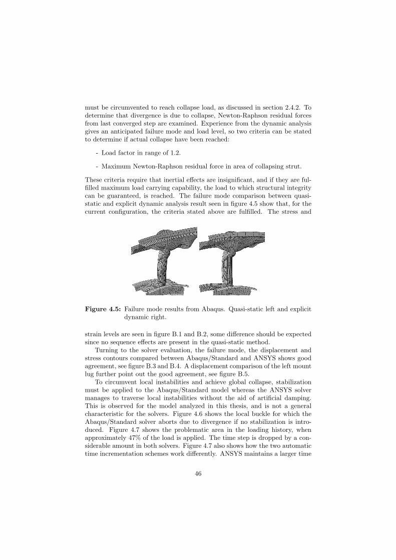
These criteria require that inertial effects are insignificant, and if they are ful-filled maximum load carrying capability, the load to which structural integritycan be guaranteed, is reached. The failure mode comparison between quasi-static and explicit dynamic analysis result seen in figure 4.5 show that, for thecurrent configuration, the criteria stated above are fulfilled. The stress and
Figure 4.5: Failure mode results from Abaqus. Quasi-static left and explicitdynamic right.
strain levels are seen in figure B.1 and B.2, some difference should be expectedsince no sequence effects are present in the quasi-static method.
Turning to the solver evaluation, the failure mode, the displacement andstress contours compared between Abaqus/Standard and ANSYS shows goodagreement, see figure B.3 and B.4. A displacement comparison of the left mountlug further point out the good agreement, see figure B.5.
To circumvent local instabilities and achieve global collapse, stabilizationmust be applied to the Abaqus/Standard model whereas the ANSYS solvermanages to traverse local instabilities without the aid of artificial damping.This is observed for the model analyzed in this thesis, and is not a generalcharacteristic for the solvers. Figure 4.6 shows the local buckle for which theAbaqus/Standard solver aborts due to divergence if no stabilization is intro-duced. Figure 4.7 shows the problematic area in the loading history, whenapproximately 47% of the load is applied. The time step is dropped by a con-siderable amount in both solvers. Figure 4.7 also shows how the two automatictime incrementation schemes work differently. ANSYS maintains a larger time
46

Figure 4.6: A typical local buckle, rendering in a too early simulation abor-tion.
increment whilst Abaqus/Standard bisects more frequently. Abaqus/Standardperforms fever equilibrium iterations for the majority of increments than AN-SYS.
0 0.2 0.4 0.6 0.8 1 1.2 1.40
0.02
0.04
0.06
0.08
0.1
0.12
0.14
0.16
Load
Load
incr
emen
t
Load incrementation
ANSYSAbaqus
Figure 4.7: Time incrementation comparison ANSYS blue andAbaqus/Standard black.
The simulation time is compared both from terminated analysis due todivergence and completed analysis run with smaller load factor, see table 4.5and 4.6. To investigate how stabilization impacts the simulation time, a ANSYSsimulation is performed with the same amount of stabilization that is appliedto the Abaqus/Standard model, see B.6. Abaqus/Standard is generally fasterthan ANSYS with one exception, when applying a lower load so that the TECdoes not collapse, i.e. convergence for all load steps. Abaqus/Standard alsoscales better to multiple CPUs, see tables 4.5 and 4.6.
47

Table 4.5: Quasi-static solution, time comparison to global collapse.
Solver, load level Time/min
1 CPU 4 CPUsAbaqus/Standard, 120% 172 61ANSYS, 119% 255 166ANSYS, 118% * 237 153* without stabilization
Table 4.6: Quasi-static solution, time comparison to 100% load.
Solver Time/min
1 CPU 4 CPUsAbaqus/Standard 114 41ANSYS 97 64
Efficiency of the equation solvers could be compared by the time it takes toperform one equilibrium iteration. This is done by dividing the simulation timefor one CPU by the total number of iterations. Abaqus/Standard performs oneequilibrium iteration in approximately 25 seconds , which is considerably fasterthan ANSYS which takes approximately 48 seconds.
4.4 Implicit dynamic
As in the quasi-static study only Model 2 is used, i.e. all shell elements arereduced integration shells.
The contribution from the inertial forces in the equilibrium equations helpsto avoid singular matrices, and thus helps to circumvent local instability prob-lems. The response from the transient excitation is very similar whether im-plicit or explicit time integration is used, see failure mode and stress distributionin figure C.1. Results coincide in terms of failure load.
Turning to the ramped loading approach, the static solution is sought witha dynamic procedure, so the dynamic forces must not affect the solution in anunwanted way. Thus the rate of which loads are ramped must be small. Loadrate is defined as load frequency divided by fundamental frequency, ωf/ω0. Inother words a measure of how “static” the simulations are. Results show thatthe rate must be below 0.12 to obtain the static solution for this structureand load case. A response consistent with the quasi-static solution method isobtained when load rate is around 0.05. In both approaches, the failure mode iscaptured and can be inspected visually in contrast to the quasi-static method.
The efficiency of the dynamic implicit methods in terms of simulation time
48

is shown in table 4.7.
Table 4.7: Simulation time, dynamic implicit.
Approach Time/min, 4 CPU Loadrate, ωf/ω0
Transient load, damping 278 *Ramped load 489 0.005Ramped load, damping 332 0.005Ramped load, damping ≈ 140 0.12* not of interest
Applying a small amount material damping, Rayliegh stiffness proportionaldamping, decreases simulation time by a considerable amount and no impacton response is observed.
49

50

Chapter 5
Conclusions
5.1 Method and accuracy
The obtained failure mode is the same independent of solver and method used,provided that the proper analyse settings has been used. This implies that thesignificance of inertial forces are small for this type of problem.
The explicit dynamic procedure, where true load transient is used and nosimplification on inertial forces are made, is a efficient way to simulate the FBOevent. The most significant drawback is the inherent limitation of time step size,see section 2.4, which in turn limits the spatial resolution of the model and thusstress and strain resolution. In the implicit dynamic procedure the time stepis not limited by spatial resolution, however it is quite costly. The alternativemethod is the quasi-static solution. In spite of a quite high frequency ratioa good agreement in collapse mode and load factor is seen between solutionmethods. One likely reason for this is that the applied loads are so large thatthey together with stiffness forces dominate the equilibrium relation.
Though failure mode is very similar, deformation evolves somewhat differ-ently between quasi-static and dynamic methods. Since the quasi-static ap-proach is simplified in terms of no load cycling, sequence effects, e.g. plasticstrain differs between methods.
The most reliable way to determine if a quasi-static method computes ac-ceptable results is to perform analysis with both solution procedures and com-pare the result. The work performed shows that a quasi-static approach is anacceptable simplification for the configuration an load studied in this thesis.
5.2 Simulation time
In the dynamic explicit simulations LS-DYNA is twice as fast as Abaqus/Explicit,however the result from the shell element evaluation, section 4.2, point out that
51

shell element type 2 gives a slightly more flexible response than other testedshell element formulations. The analyst should be aware of this when deter-mining which shell formulation to use. The Abaqus/Explicit solver computesequivalent collapse load factor regardless of shell element type. This impliesthat when comparing Abaqus/Explicit Model 1 and LS-DYNA Model 2 resultsand simulation time corresponds.
For the quasi-static analysis Abaqus/Standard is generally faster than AN-SYS. However, if the analysis is not driven to the global limit point, i.e. con-vergence on all load steps, ANSYS is somewhat faster than Abaqus/Standard.This may not be directly meaningful for buckling analysis but indicates thatmodifications to ANSYS’s default time incrementation scheme might speed upsolution time for this type of analysis.
Abaqus/Standard experiences difficulties traversing local buckles for themodel analysed in this thesis. A permitted higher number of equilibrium itera-tions before convergence check, to prevent premature cutback, does not seem tohelp. No correlation between the solvers convergence criteria and their imple-mentation has been done. It is likely that they differ from each other, and couldbe one reason why Abaqus/Standard needs stabilization and ANSYS does not.However, other models analysed at Volvo Aero has shown difficulties with localinstabilities in ANSYS.
To perform quasi-static buckling analysis, experience of the structures re-sponse is very useful. Applying the right amount of stabilization, if needed, andsetting time incrementation parameters can be difficult if no previous knowl-edge is at hand.
When it comes to the experimentation with the implicit dynamic procedure,two different conclusions is drawn. The ramped load approach is not a preferredmethod, since it is time costly to use a sufficiently long timescale to obtain thestatic solution and avoid unwanted dynamic effects. If time scale is to short,it may render in a wrong problem being solved. The time step is limited byconvergence issues, caused by high frequency panel modes at the outer caseof the TEC. Thus the problem with using the ramped load approach is thatthe ratio between the period time of the fundamental mode and the highermodes is large. The time scale must be substantially longer than the periodtime of the fundamental mode, but the time step size is limited by convergenceissues caused by the higher modes of vibration. This observation implies thatresolving the FBO transient is not an issue due to the small time step causedby the structural response, leading to the second conclusion. The dynamicprocedure should be used to analyze the transient response and not the staticresponse.
For the element size used in this thesis the explicit procedure is considerablyfaster, although at some point of model refinement the two methods shouldcoincide in terms of simulation time. The possibility to perform sub-modelanalysis will affect the choice of solution technique.
52

Chapter 6
Further work
As the thesis has shown, both quasi-static and dynamic methods are feasible.The ability to change solution method during analysis could be useful to tra-verse local buckles. The implicit solver in LS-DYNA has not been evaluated inthis thesis. The work performed however, can be used as a starting point forsuch studies.
As the element stiffness differ somewhat in this study, it is recommendedto perform a mesh convergence study for the sub-model. Then a componentstiffness test, similar to the stiffness test in section 4.2, could be used to validatewhich shell element is most appropriate for the structure.
Reducing simulation time for the implicit dynamic method could be investi-gated with following measures. Specifying the material damping for individualparts, e.g. a larger amount of damping could be applied to panels that expe-riences high frequency vibration, or selectively scale the mass of these parts toreduce their frequency of vibration.
53

54

Appendix A
Figures. Explicit dynamic
Figure A.1: von Mises stress Model 1, aft looking forward. LS-DYNA leftand Abaqus/Explicit right.
55
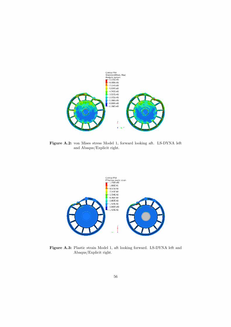
Figure A.2: von Mises stress Model 1, forward looking aft. LS-DYNA leftand Abaqus/Explicit right.
Figure A.3: Plastic strain Model 1, aft looking forward. LS-DYNA left andAbaqus/Explicit right.
56

Figure A.4: Plastic strain Model 1, forward looking aft. LS-DYNA left andAbaqus/Explicit right.
Figure A.5: von Mises stress Model 2, aft looking forward. LS-DYNA leftand Abaqus/Explicit right.
57

Figure A.6: von Mises stress Model 2, forward looking aft. LS-DYNA leftand Abaqus/Explicit right.
Figure A.7: Plastic strain Model 2, aft looking forward. LS-DYNA left andAbaqus/Explicit right.
58

Figure A.8: Plastic strain Model 2, forward looking aft. LS-DYNA left andAbaqus/Explicit right.
0 0.02 0.04 0.060
5
10
15
20
25Bearing resultant displacement
Time / sec
Disp
lace
men
t / m
m
LS−DynaAbaqus
0 0.02 0.04 0.060
5
10
15
20
25
30Right lug resultant displacement
Time / sec
Disp
lace
men
t / m
m
LS−DynaAbaqus
Loadfactor 125%
0 0.02 0.04 0.060
50
100
150Left lug resultant displacement
Time / sec
Disp
lace
men
t / m
m
LS−DynaAbaqus
Figure A.9: Resultant displacement for mount lugs and bearing, Model 1.
59

0 0.01 0.02 0.03 0.04 0.05 0.06 0.070
2
4
6
8
10
12
14
16
18x 107 External work, Loadfactor 125%
Time / sec
Ener
gy /
mJ
LS−DynaAbaqus
Figure A.10: External work, 125% load factor, Model 1.
0 0.02 0.04 0.060
2
4
6
8
10x 105 Left upper strut resultant force
Time / sec
Forc
e / N
LS−DynaAbaqus
0 0.02 0.04 0.060
2
4
6
8
10
12x 105 Right upper strut resultant force
Time / sec
Forc
e / N
LS−DynaAbaqus
0 0.02 0.04 0.060
2
4
6
8x 10⁴ Left lower strut resultant force
Time / sec
Forc
e / N
LS−DynaAbaqus
Loadfactor 125%
0 0.02 0.04 0.060
0.5
1
1.5
2x 10⁵ Right lower strut resultant force
Time / sec
Forc
e / N
LS−DynaAbaqus
Figure A.11: Resultant section forces, Model 1.
60

0 0.05 0.1 0.15 0.2 0.250
1
2
3
4
5
6
7
8x 10⁷ External work, Loadfactor 119%
Time / sec
Ener
gy /
mJ
LS−DynaAbaqus
Figure A.12: External work, 119% load factor, Model 1.
Figure A.13: External work. LS-DYNA only shell type 16. Abaqus/ExplicitModel 1.
0 0.1 0.2 0.3 0.4 0.5 0.6 0.7 0.8 0.9 10
2
4
6
8
10
12x 105
Displacement / mm
Fore
ce /
N
Type 2,LS−Dyna,IHQ=1Type 2, LS−Dyna,IHQ=4
Figure A.14: Sub-model reaction forces for different hourglass formulation.Red is viscous and blue is stiffness based.
61

0 0.1 0.2 0.3 0.4 0.5 0.6 0.7 0.8 0.9 10
2
4
6
8
10
12x 105
Displacement / mm
Fore
ce /
N
S4, AbaqusS4RS, AbaqusType 2, LS−DynaType 16, LS−DynaType 10, LS−Dyna
Figure A.15: Sub-model reaction force for different shell types.
62

Appendix B
Figures. Quasi-static
Figure B.1: von Mises stress. Explicit dynamic method left and quasi-staticmethod right.
63

Figure B.2: Plastic strain. Explicit dynamic method left and quasi-staticmethod right.
Figure B.3: Displacement, 3 times magnified. ANSYS left andAbaqus/Standard right.
64

Figure B.4: von Mises stress. ANSYS left and Abaqus/Standard right.
Figure B.5: Displacement of left mount lug. ANSYS blue andAbaqus/Standard black.
65

0 0.2 0.4 0.6 0.8 1 1.2 1.40
0.5
1
1.5
2
2.5
3
3.5
4
4.5
5x 10⁴ Dissipated energy
Time
Ener
gy /
j
AbaqusANSYS
Figure B.6: Dissipated stabilization energy. ANSYS blue andAbaqus/Standard black.
66

Appendix C
Figures. Implicit dynamic
Figure C.1: von Mises stress dynamic analysis. Explicit left and implicitright.
67

68

Appendix D
Analysis equipment
The computer used:
- Two Dual Core Intel X5260 @ 3.33 GHz processors
- 8 GB RAM
- Hitachi Ultrastar 15K300 SAS 3.0 Gb/s hard drive dedicated for thesimulations
Finite element solvers used:
- LS-DYNA 971 rev 1224 SMP
- Abaqus 6.8-1
- ANSYS 11.0
69

70
Bibliography
[1] MTU Aero Engines GmbH
[2] Bathe, K. J., “Finite Element Procedures”, Prentice-Hall, 1996
[3] Hinton, E., “Introduction to Nonlinear Finite Element Analysis”,NAFEMS, 1992.
[4] Hilber, H. M., Huges, T. J. R. and Taylor, R. L., “Collocation, Dissipa-tion and ‘Overshoot’ for Time Integration Schemes in Structural Dynam-ics”, Earthquake Engineering and Structural Dynamics, Vol. 6, pp. 99-117,1978.
[5] Griffiths, D. V. and Mustoe, G. G. W., “Selective Reduced Integration ofFour-Node Plane Element in Closed Form”, Journal of Engineering Me-chanics, Vol. 121, No. 6, pp. 725-729, June 1995.
[6] LSTC Inc, Engineering Research Nordic AB and DYNAmore GmbH
[7] Belytschko, T., Lin, J. I. and Tsay, C. S. “Explicit Algorithms for theNonlinear Dynamics of Shells”, Computer Methods in Applied Mechanicsand Engineering, Vol. 42, pp. 225-251, 1984.
[8] LS-DYNA Theory Manual 2006
[9] Abaqus Analysis User’s Manual v6.8
71