2008:133 CIV

M A S T E R ' S T H E S I S

Fluid Flow in Microgeometries

Anders G. Andersson

Luleå University of Technology

MSc Programmes in Engineering Engineering Physics

Department of Applied Physics and Mechanical EngineeringDivision of Fluid Mechanics

2008:133 CIV - ISSN: 1402-1617 - ISRN: LTU-EX--08/133--SE

2

Preface

This thesis is the result of work carried out at the Division of Fluid Mechanicsat Luleå University of Technology as a part of the Research Trainee programduring August 2007 - May 2008. The project was partially funded by theNanofun-Poly Network of Excellence.

I would like to acknowledge some important people who made this thesis pos-sible. First of all I would like to acknowledge my supervisor professor StaffanLundström for giving me the oppurtunity to work with this project and alot oftactical advice. I would also like to acknowledge associate professor ThanasisPapathanasiou at University of South Carolina for supplying the experimentalchannels and for bringing alot of enthusiasm and ideas on the experimentalwork. I would like to thank PhD student Torbjörn Green and PhD Lars-GöranWesterberg for the assistance with the experiments and the divisions technicianAllan Holmgren who helped greatly with all the practical issues which alwaysoccurs when working in a lab enviroment.

Anders AnderssonLuleå, June 17, 2008

i

ii

Abstract

The flow in micro geometries is of interest in applications such as bioanalysissystems, micro-valves and flow through porous media. The flow is generallystraight-forward to predict since the flow is laminar and the geometries areoften simple. However when it comes to flow through dual scale porous me-dia, the flow gets harder to predict. The flow through porous media can beapplied to areas such as composites manufacturing, paper making and dryingof iron ore pellets. The aim of this project is therefore to study flows in microgeometries with numerical and experimental methods to gain increased under-standing of porous media flow. The optical method best suited for this kindof geometries is micro particle image velocimetry(µ-PIV) and the numericalcalculations are done with computational fluid dynamics(CFD). µ-PIV is usedto investigate the flow in channels with a single fibre and with fibre arrays ofdifferent patterns and densities. The effect permeability has on flow fields inchannels is investigated with CFD.

iii

iv

Contents

Preface i

Abstract iii

Nomenclature 1

1 Introduction 31.1 Porous media . . . . . . . . . . . . . . . . . . . . . . . . . . 41.2 Optical measuring methods . . . . . . . . . . . . . . . . . . . 51.3 Computational Fluid Dynamics . . . . . . . . . . . . . . . . . 5

2 Method 72.1 Particle Image Velocimetry . . . . . . . . . . . . . . . . . . . 7

2.1.1 Seeding Particles . . . . . . . . . . . . . . . . . . . . 82.2 Experimental setup . . . . . . . . . . . . . . . . . . . . . . . 92.3 Numerical models . . . . . . . . . . . . . . . . . . . . . . . . 12

2.3.1 Flow around single fibre . . . . . . . . . . . . . . . . 122.3.2 Flow through fibre bundle . . . . . . . . . . . . . . . 13

3 Results 153.1 Flow around single fibre . . . . . . . . . . . . . . . . . . . . 153.2 Flow through fibre bundles . . . . . . . . . . . . . . . . . . . 17

3.2.1 Rectangular fibre array . . . . . . . . . . . . . . . . . 173.2.2 Hexagonal fibre array . . . . . . . . . . . . . . . . . . 20

4 Discussion 25

v

vi CONTENTS

Bibliography 28

Nomenclature

K̄ Permeability tensor, m2

∆t Measurement time interval, s

εB Relative error due to Brownian motion

µ Dynamic viscosity, Pa · s

ν Kinematic viscosity, m2/s

νs Superficial velocity, m/s

ρ Density, kg/m3

Ac Cross-sectional area, m2

Dh Hydraulic diameter, m

p Pressure, Pa

pw Wetted perimeter

u Velocity, m/s

D Einsteins diffusion coefficient, m2/s

f Fibre volume fraction

R Fibre radius, m

1

2 CONTENTS

Chapter 1Introduction

There is said that fluid flows has two states. When the flow is said to be lam-inar, it means that the flow is highly ordered and has smooth streamlines. Astreamline is defined as a curve that is everywhere tangent to the instantaneouslocal velocity vector. When flow has velocity fluctuations and disordered mo-tion, the flow is said the be turbulent. There are several parameters that affectthe transition from laminar to turbulent flow, for instance the geometry, fluidvelocity and material properties of the fluid. The experimental work of Os-borne Reynolds in the 1880’s led to the conclusion that the transition could bedescribed as a ratio of the inertial forces to viscous forces in the fluid. Thisratio is known as the Reynolds number and is defined as

Re =uDh

ν(1.1)

where u [m/s] is the average velocity of the flow, ν [m2/s] is the kinematicviscosity and Dh [m] is the hydraulic diameter. The hydraulic diameter isdefined as

Dh =4Ac

pw(1.2)

where Ac [m2] is the total cross-sectional area of the flow and p is the wettedperimeter.

In the case of flow through microgeometries the flow is laminar in almost ev-ery case because of the small scales involved.

3

4 CHAPTER 1. INTRODUCTION

The flow can be described by the equations of fluid motion. The continuityequation and the Navier-Stokes equation is defined as follows

∂ρ

∂t+∇ · (ρu) = 0 (1.3)

ρ

(∂u∂t

+(u ·∇)u)

=−∇p+µ∇2u (1.4)

where ρ [kg/m3] is the density of the fluid, p [Pa] is the pressure and µ [Pa·s]is the dynamic viscosity. If the fluid is considered incompressible or in otherwords ρ is constant, the continuity equation reduces to

∇ ·u = 0 (1.5)

Solving Navier-Stokes equation for anything except simple flow fields is notpossible at present time since it is an time dependant, nonlinear, second or-der partial differential equation[1]. Since analytical solutions are not possiblefor more complex cases it is therefore of great interest to analyze these casesexperimentally or numerically.

1.1 Porous media

The flow in porous media has been of interest for a long time. Henry Darcystudied the filtering of drinking water in the city of Dijon as early as in 1856.From the experimental observations he derived a one-dimensional law for flu-ids propagating through a porous media. His law was theoretically derived andextended to several dimensions to take the form

νs =−K̄µ

∇p (1.6)

where νs [m/s] is the superficial velocity(ratio between volumetric flow ratethrough the porous medium and the cross-sectional area in the flow direction)and K̄ [m2] is the permeability tensor of the porous medium[2]. The law isvalid as long as the Reynolds number is low enough to ensure a totally lami-nar flow, the fluid is incompressible and Newtonian and the porous domain isstationary.

1.2. OPTICAL MEASURING METHODS 5

A Newtonian fluid is defined as as a fluid for which the shear stress is lin-early proportional to the shear strain rate. This can be compared to the elasticsolids where the stress can be described as a material constant times the strain.

1.2 Optical measuring methods

Optical measuring methods have been used for several years. These kinds ofmethods are well suited for fluid mechanical problems since mechanical meth-ods tend to disturb the flow. Among the first to use tracker particles to mon-itor flows was Ludwig Prandtl. In the beginning of the 1900s he performedexperiments on flow around objects in a water tunnel where particles was in-troduced to the surface of the flow. From these experiments Prandtl was ableto show flow phenomena in a qualitative way. With the development of tech-nology in the last couple of decades, mostly the transition to digital recordingand evaluation have given the optical measurement techniques the ability togive quantitative data such as velocities. Particle image velocimetry or Laserspeckle velocimetry as it was called early on started to develop in the late 70sand early 80s. In the early work of Roland Meynart he showed that it waspossible to make practical measurements on both laminar and turbulent flowof fluids with this method[3, 4]. The concept of applying this technique to submillimeter scaled geometries started developing in 1998 where the flow aroundan elliptical cylinder with a major diameter of 30 µm was investigated[5]. Theflow through rectangular networks of cylinders has been investigated with thePIV-method where different solid volume fractions and fibre radii was lookedat[6, 7].

1.3 Computational Fluid Dynamics

Solving fluid related problems numerically with Computational Fluid Dynam-ics has become a standard industral tool. Solving the Reynolds-AveragedNavier-Stokes(RANS) equations with the help of computers is considered agood method on solving problems that are too complex to solve analytically. Itis important to understand that the solutions obtained from CFD will always beapproximate because a CFD model is always a simplification of reality. Therewill be model uncertainties which are the difference between the exact solu-tions of the solved equations and the actual flow, there will be discretisation or

6 CHAPTER 1. INTRODUCTION

numerical errors since the geometry is discretised and only the discretised ver-sions of the continuum transport equations and energy transfer can be solvednumerically and when these equations are solved numerically there will be it-eration or convergence errors. The iteration and convergence errors are thedifference between the fully converged solution on the numerical grid and asolution which is not fully converged due to lack of time or inadequate nu-merical methods. Since computers have a limits for how many digits they canstore for a parameter value there will always be some kind of round-off errorin CFD-results as well[8].There is different approaches on how to discretize numerical models for CFD.The easiest method to apply to simple geometries is the Finite Differencemethod(FD). This method can be applied to any type of grid but it is mostly as-sociated with structured grids. The basic principle for FD is that Taylor seriesexpansions or polynomial fitting is used to find approximations of the first andsecond order derivates of the investigated variables in the coordinates that arelocated along the grid lines. The downsides of FD is that it does not enforceconservation and that is restricted to simple geometries.With the Finite Volume Method(FV), the solution domain is divided into con-trol volumes(CVs), and the conservation equations are solved applied to eachCV. The integral form of the conservation equations is used which also meansthat conservation will always be maintained. Surface and volume integrals areapproximated which gives values in nodes in the centroid of each CV and in-terpolation gives values on the CV surface. The main disadvantage with FVis that it is hard to develop methods of order higher than two for three dimen-sional cases.The Finite Element method(FE) uses a similar approach as FV with the maindifference being that the equations are multiplied with weight functions beforethey are integrated over the domain. The FE method is also mostly associatedwith unstructured grids[9]. There is also hybrid methods between FE and FVwhich is used by commerical software such as ANSYS CFX.

Computational fluid dynamics can be applied to the flow through porous me-dia in several ways. A finite volume approach can be used to calculate thepermeability of cells with a geometry typical for composite materials[10] orfor a given permeability, calculate important physical variables such as veloc-ities or temperatures. There are other ways to model flows through porousmaterials which will allow one to model every fibre in a fibre bundle e g theBoundary Element Method were flows through bundles of circular fibres hasbeen investigated[11, 12].

Chapter 2Method

2.1 Particle Image Velocimetry

Particle Image Velocimetry is a method that allows complex instantaneousvelicty fields to be measured[13]. In a typical PIV-setup the flow is seededwith tracer particles and a plane is illuminated two times or more in a shortperiod of time. The emitted light from the particles are then recorded by acamera. The recordings are evaluated on a computer by dividing the imagesinto smaller subareas and comparing the particle placement in these subareas.The assumtion is made that the particles move linearly within the subarea whenthe time between images ∆t is sufficiently small. By correlating the particlesplacement in sequential images, both the magnitude of the velocity and the di-rection can be evaluated, see Fig. 2.1.

One disadvantage with conventional two-dimensional PIV is that it only ac-counts for the particles that move in the investigated plane. Particles that moveinto or out of that plane will cause problems in the correlation and give corruptdata to the obtained results.

When applying the PIV technique to microgeometries some adjustments mustbe made. The investigated domain is imaged through a microscope before itis captured by the camera. Since the illumination of a single plane is difficultto achieve in these kinds of geometries the entire volume is illuminated by thelight source. The limitation in measurement depth is instead decided by thefocus of the microscope.

7

8 CHAPTER 2. METHOD

Figure 2.1: Basic principle behind cross-correlation

2.1.1 Seeding Particles

The seeding particles have a big impact on how the results of an experimentwill turn out. Both the size of the particles and the particle concentration areparameters that should be chosen in such a way that they match the studiedgeometry and flow velocity. The particles should be small enough to followthe flow in a good way but not so small that they will be affected by randomdisturbances in their movement which is known as Brownian motion. Therelative error that occurs from Brownian motion can be estimated by

εB =1u

√2D∆t

(2.1)

where D [m2/s] is Einsteins diffusion coefficient and ∆t [s] is the measurementinterval[5].

The particle concentration should be kept as low as possible to keep a goodsignal-to-noise ratio[14]. This is because the number of particles that moveoutside the investigated plane is lower and their emitted light will not add asmuch noise to the pictures obtained. Since low particle concentrations canlead to insufficient data to perform correlations between two consecutive im-ages the "‘Sum of Correlations method"’ was used. This method will sum upan arbitrary number of correlations before the velocity field is calculated[15].

Parafin oil was used as fluid in all experiments because it has a refraction index

2.2. EXPERIMENTAL SETUP 9

close to that of the glass walls of the channels. It is important to have a ho-mogenous particle distribution in the fluid. If particles start to clump togetherthey will disturb the velocity field obtained from the experiments. When mix-ing the particles into the parafin oil special care has to be taken or alot of airwill be added to the fluid. Since the air bubbles generally are larger than thetracer particles they will have a significant negative effect on the results. Thefirst method was simple to apply the particles to the surface of the containerthat held the fluid and then stir. With the stirring method alot of air is trappedinside the fluid and alot of particles adhere to the walls. The method thatseemed to give the best fluid was to use a sonic bath for the mixing. Placingthe container with the fluid and tracker particles in the sonic bath where smallvibrations handled the mixing gave a very homogenous distribution of parti-cles in the fluid. The procedure does however add some air to the mixture andthis had to be dealt with in some way. The solution was to put the containerwhich held the mixtrure in a vacuum pump to get rid of all the residual air.

2.2 Experimental setup

The light source used in the expermients was a pulsed Nd:YAG laser fromLitron Lasers emitting light at a wavelength of λ = 532nm. The images arepictured through a Zeiss Axiovert 200 microscope. The seeding particles usedwas 10.2 ±0.17µm Rhodamine B particles from Microparticles GmbH. In or-der to get a constant volume flow into the inlet of the channel, a KDS Model100 Series pump was used. The experimental setup can be seen in Fig. 2.2.

Figure 2.2: Experimental setup[16]

Several experimental cells was constructed to investigate fluid flow in microge-ometries. The geometry consists of an inlet pipe with R = 0.6 mm which leadsto a 1.6 mm wide slit designed to remove three dimensional effects which inturn ends up in the main channel with dimensions 5.3x7x7 mm3. The main

10 CHAPTER 2. METHOD

channel has a porous region, in reality consisting of an array of fibres, whichis 4 mm wide and 4 mm long and takes up the entire channel depth. The fibresare shaped as cylindrical rods and have a radius of 150µm. Open regions areleft around the fibre array to allow different flow phenomena to be investigated.Several top plates with pre-drilled holes in different formations were used forattaching the fibres. Since the channel consists of several parts and the topand bottom plates are replaceable there will always be a risk for leakage. Thechannel must be filled before it is sealed to make sure no air is trapped insidethe cavity. A thin layer of a two component epoxy glue was applied to theedges of the top and bottom plates to make them completely sealed shut. Eventhe smallest leak will cause air to enter the channel and the measurement to beruined. This will also lead to that the channel must be taken apart and refilledwhich can be very time-consuming.To see how well the PIV handled the small fibres the first experiment containedonly one single fibre attached to the top plate and the flow around it was inves-tigated both experimentally and numerically.Another experiment was carried out when the fibres was arranged as an rect-angular array with a relatively low solid fraction. The final experiment was theflow through and around a much denser hexagonally arranged fibre array. Anoptical view of the hexagonal fibre array can be seen in Fig. 2.3.

2.2. EXPERIMENTAL SETUP 11

Figure 2.3: Optical view of fibre bundle

12 CHAPTER 2. METHOD

2.3 Numerical models

2.3.1 Flow around single fibre

The geometry for the numerical model of the flow around one fibre was createdin ANSYS Workbench and the unstructured mesh was created in ICEM CFD.The unstructured mesh had 737k tetrahedral elements. A local refinement nearthe cylinder was applied to give increased accuracy near the cylinder surface,see Fig. 2.4.

Figure 2.4: Mesh

The inlet boundary condition is set as a plug profile with velocity obtained fromexperimental data. The cylinder and the top and bottom walls are modelledwith a no slip boundary condition and the front and back walls are modelledas symmetry planes to remove wall effects. The outlet uses an average staticpressure of 0Pa. The root mean square(RMS) residual targets was set to 1e-6 which is very tight convergence suitable even for geometrically sensitiveproblems[17].

2.3. NUMERICAL MODELS 13

2.3.2 Flow through fibre bundle

The geometry for the channel with the porous material was the same as the ge-ometry of the channel used in the experiments with the fibre bundles. The ge-ometry was created and a block structured mesh was created which had 1470knodes. The block structure for the mesh was built up by a O-grid which startsat the inlet and goes all the way to the outlet and the areas around the O-gridwas meshed as homogenous as possible. The geometry and the mesh can beseen in Fig. 2.5(a) and 2.5(b) respectively.

(a) Geometry (b) Mesh

Figure 2.5: Geometry and mesh for numerical model

The velocity at the inlet was set to a plug profile with velocity correspondingto the inlet velocity of the experiments. A plug profile is not a very realisticassumption but it was considered a reasonable approximation since a fully de-veloped profile will be obtained very soon in the tiny capillary leading to thecavity. All walls were modelled with a no-slip boundary condition. The outletwas set to use an average static pressure of 0Pa. The fibre bundle was modelledas a porous subdomain with constant permeabilty. This approach was chosenbecause it’s easier to model a complex 3D structure this way than to modelevery fibre in the fibre bundle. The permeability for hexagonal fibre arrays canbe calculated as

K|| =8C

(1− f )3

f 2 R2 (2.2)

K⊥ = C

(√fmax

f−1

)(5/2)

R2 (2.3)

14 CHAPTER 2. METHOD

where f is the fibre bundle volume fraction, C is a constant close to unity thatis dependent on the actual fibre arrangement and R [m] is the fibre radius[18].

Chapter 3Results

3.1 Flow around single fibre

The velocity field obtained from PIV and the one obatined from CFD can beseen in Fig. 3.1(a) and 3.1(b) respectively. The results looks very similarand the flow is much like what one would expect for flows with low reynoldsnumbers. With very low upstream velocities the fluid completely wraps thecylinder and the flow going above the cylinder and the flow going beneath itwill meet behind the cylinder in an ordered manner. For RE ≥ 10 there willbe some separation that starts occuring behind the cylinder but in this case RE≤ 1 and hence no separation will occur.

15

16 CHAPTER 3. RESULTS

(a) Experimental

(b) Numerical

Figure 3.1: Velocity fields

3.2. FLOW THROUGH FIBRE BUNDLES 17

3.2 Flow through fibre bundles

3.2.1 Rectangular fibre array

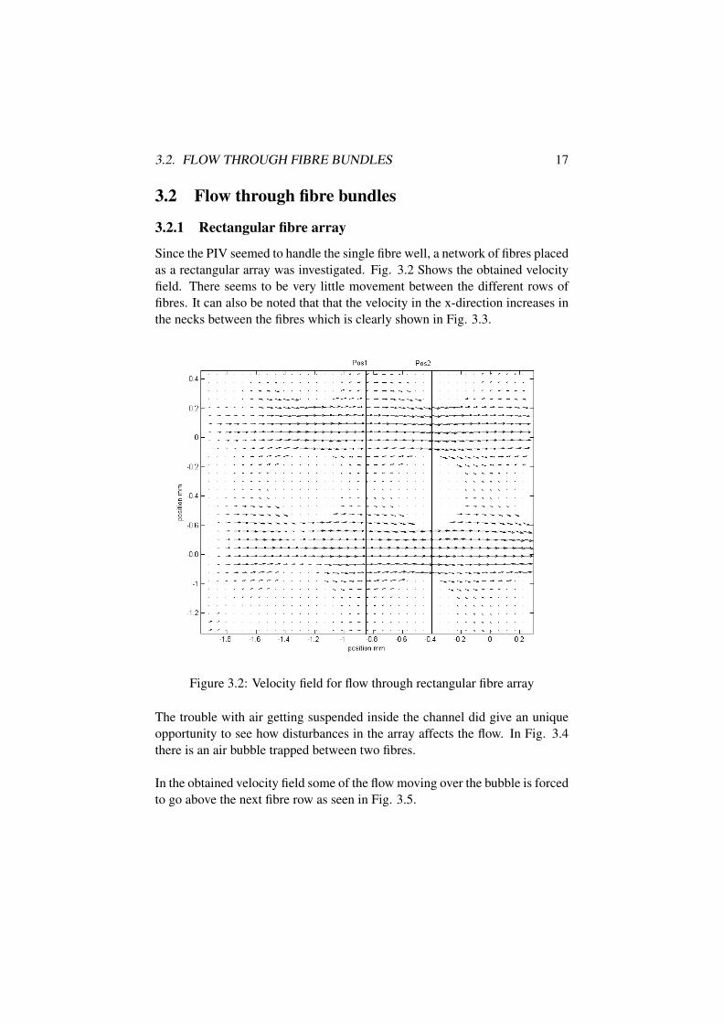
Since the PIV seemed to handle the single fibre well, a network of fibres placedas a rectangular array was investigated. Fig. 3.2 Shows the obtained velocityfield. There seems to be very little movement between the different rows offibres. It can also be noted that that the velocity in the x-direction increases inthe necks between the fibres which is clearly shown in Fig. 3.3.

Figure 3.2: Velocity field for flow through rectangular fibre array

The trouble with air getting suspended inside the channel did give an uniqueopportunity to see how disturbances in the array affects the flow. In Fig. 3.4there is an air bubble trapped between two fibres.

In the obtained velocity field some of the flow moving over the bubble is forcedto go above the next fibre row as seen in Fig. 3.5.

18 CHAPTER 3. RESULTS

Figure 3.3: velocity profiles for flow through rectangular fibre array

Figure 3.4: Air bubble trapped between fibres

3.2. FLOW THROUGH FIBRE BUNDLES 19

Figure 3.5: Velocity field of array with air bubble

20 CHAPTER 3. RESULTS

3.2.2 Hexagonal fibre array

Since the difference in velocities of the flow moving through the bundle andthe flow moving around it is so large it will be difficult to cross correlate theparticles movements both inside the bundle and around it on the same picture.The flow around the fibre bundle is shown in Fig. 3.6 where three fibres canbe vaguely spotten in the upper part of the plot.

Figure 3.6: Velocity field ouside fibre bundle

In order to get as small contribution as possible from particles that move intoor out of the measurement plane it is desired to put the measurement planewhere the flow has the smallest variations in the direction perpendicular toit. Fig. 3.7 shows streamlines for the flow in the plane perpendicular to themeasurement plane obtained from the numerical simulations. As it can beseen the optimal places to measure would be in the symmetry plane or close tothe top or bottom wall. The symmetry plane would be more suitable becausethe velocity near the walls is very slow and there might be some wall effectpresent. Due to geometrical limitations for the channels and the microscopethis was not possible at first and because of this, the flow was captured close tothe bottom wall. The cross-correlated image of a measurement series is shownin Fig. 3.8. The results show that we have flow moving further into the porousbundle and also out into the bulk flow which can be seen in the upper part ofthe figure.

3.2. FLOW THROUGH FIBRE BUNDLES 21

Figure 3.7: Streamlines for velocity in plane perpendicular to measurementplane

Figure 3.8: Fluid flow through fibre bundle

22 CHAPTER 3. RESULTS

In order to investigate the flow at a greater distance from the microscope lence,a holder for the channel was constructed. The holder allowed the channel tobe lowered so it was closer to the microscope lence which increased the mea-surement depth. The holder was made out of PMMA and it had four screwsto stabilize the channel and help keep it horisontal. The velocity profile insidethe bundle obtained near the middle of the channel can be seen in Fig. 3.9.

Figure 3.9: Velocity profile near middle of channel

The velocity obtained from the numerical simulations in the plane in the cen-ter of the channel is shown in Fig. 3.10(a). Since the difference in velocitybetween the flow going through the bundle and the flow going around it israther large, a logarithmic scale was chosen for the velocity. A close-up onthe porous domain is shown in Fig. 3.10(b). It can be observed that there is aslightly higher velocity near the corners of the bundle which implies that someof the flow is forced to pass through the bundle there.

An investigation was made on how the permeability of the porous domain af-fects the flow in the channel. The original permeability that was calculatedfrom the experimental cell was used as a base and was compared to simula-tions that hade that permeability increased by 100 times and 1000 times. Theresults of that investigation can be seen in Fig. 3.11

This shows that the permeability of the porous domain greatly affects the be-

3.2. FLOW THROUGH FIBRE BUNDLES 23

(a) Channel (b) Porous domain

Figure 3.10: Contour plot at the porous domain

haviour of the flow in the channel. When the permeability is 100 times greaterthan for the experimental cell, the difference in velocities between the flowthrough the bundle and around it are significantly less but the parabolic shapesof the bulk flow are still very prominent. For the case of 1000 times perme-ability the flow inside the bundle is higher than for the flow around it and thevelocity profile is approaching the parabolic shape of a velocity profile forregular channel flow.

24 CHAPTER 3. RESULTS

Figure 3.11: Velocity profile in the channel for different permeabilities

Chapter 4Discussion

Micro particle image velocimetry and computational fluid dynamics was usedto investigate flows in simple sub millimeter geometries. Since reasonableresults were obtained the more complex case of porous media was looked at.The porous material in the experiments consisted of fibre arrays in differentalignments and solid volume fractions. The obtained flow fields from PIVshows that the technique can be used even in very dense arrays where thevelocities are very slow compared to the bulk flow. Although all the studiesperformed with the PIV was considered stationary, the results obtained indicatethat it should be possible to monitor flows in transient applications such as flowfronts in filling processes. It should also be possible to mix larger particlesin the fluid to see how they hinder the fluids propagation through the porousmedia. When looking at transient events there will be little to no room foroptimizing settings after the measurement has started and parameters such aslaser power, microscope focus and time between laser pulses all have greatimpact on the final results. One way to handle this would be to run a stationarycase first to evaluate the different parameters and selecting optimal settings forthem.Numerical simulations was carried out with the porous media modelled withconstant permeability according to analitycal formulas. The results showedthat the permeability of the porous material affected the flow field both insidethe fibre bundle but also the flow around it. This kind of simulations couldbe used with more complex models for permeability or porosity in order toget physical properties such as velocities or temparatures. It should also bepossible to use this method to run transient simulations where flow fronts could

25

26 CHAPTER 4. DISCUSSION

be examined over time. Another interesting aspect would be to add particles tothe fluid and use particle tracking to monitor their movement through the flowdomain.

Bibliography

[1] Y. A. Cengel and J. M. Cimbala, Fluid Mechanics: Fundamentals andApplications. McGraw-Hill, 2006.

[2] J. Bear, Dynamics of Fluids in Porous Media. American Elsevier Pub-lishing Company, 1972.

[3] R. Meynart, “Equal velocity fringes in a rayleigh-benard flow by aspeckle method,” Appl. Opt., vol. 19, no. 9, p. 1385, 1980.

[4] R. Meynart, “Speckle velocimetry study of vortex pairing in a low-Reunexcited jet,” Physics of Fluids, vol. 26, pp. 2074–2079, 1983.

[5] J. G. Santiago, S. T. Wereley, C. D. Meinhart, D. J. Beebe, and R. J.Adrian, “A particle image velocimetry system for microfluidics,” Exper-iments in Fluids, vol. 25, pp. 316–31, 1998.

[6] M. Agelinchaab, M. F. Tachie, and D. W. Ruth, “Velocity measurementof flow through a model three-dimensional porous medium,” Physics ofFluids, vol. 18, no. 1, p. 017105, 2006.

[7] W. H. Zhong, I. G. Currie, and D. F. James, “Creeping flow through amodel fibrous porous medium,” Experiments in Fluids, vol. 40, pp. 119–126, Jan. 2006.

[8] ERCOFTAC Special Interest Group, Quality and Trust in IndustrialCFD: Best Practice Guidelines. 2000.

[9] J. H. Ferziger and M. Peric, Computational Methods for Fluid Dynamics.Springer-Verlag, 2002.

27

28 BIBLIOGRAPHY

[10] M. Nordlund, T. S. Lundström, V. Frishfelds, and A. Jakovics, “Per-meability network model for non-crimp fabrics,” Composites Part A,vol. 37A, pp. 826–835, 2006.

[11] X. Chen and T. D. Papathanasiou, “Micro-scale modelling of axial flowthrough unidirectional disordered fiber arrays,” Composites Science andTechnology, vol. 67, pp. 1286–1293, 2007.

[12] X. Chen and T. D. Papathanasiou, “The transverse permeability of disor-dered fiber arrays: A statistical correlation in terms of the mean interfiberspacing,” Transport in Porous Media, vol. 71, pp. 233–251, 2008.

[13] M. Raffel, C. Willert, and J. Kompenhans, Particle Image Velocimetry: APractical Guide. Springer-Verlag, 1998.

[14] C. D. Meinhart, S. T. Wereley, and M. H. B. Gray, “Volume illumina-tion for two-dimensional particle image velocimetry,” Meas. Sci. Tech-nol., vol. 11, pp. 809–814, 2000.

[15] LaVision GmbH, DaVis Flowmaster Software manual. LaVision GmbH,Göttingen, Germany, 2005.

[16] M. Nordlund, Permeability Modelling and Particle Deposition Mecha-nisms Related to Advanced Composites Manufacturing. Luleå Universityof Technology, PhD thesis, 2006.

[17] ANSYS, CFX 11.0 Documentation. Ansys Inc, 2006.

[18] B. R. Gebart, “Permeability of unidirectional reinforcements for rtm,”Journal of Composite Materials, vol. 26, no. 8, pp. 1100–1133, 1992.