2013-06 uav swarm tactics: an agent-based simulation and ... · agent-based simulation allows for...
TRANSCRIPT

Calhoun: The NPS Institutional Archive
Theses and Dissertations Thesis Collection
2013-06
UAV swarm tactics: an agent-based
simulation and Markov process analysis
Gaerther, Uwe
Monterey, California: Naval Postgraduate School
http://hdl.handle.net/10945/34665


THIS PAGE INTENTIONALLY LEFT BLANK


THIS PAGE INTENTIONALLY LEFT BLANK
ii

Approved for public release; distribution is unlimited
UAV SWARM TACTICS: AN AGENT-BASED SIMULATION AND MARKOVPROCESS ANALYSIS
Uwe GaertnerCaptain, German Army
Diplom, University of the German Armed Forces Munich, 2004
Submitted in partial fulfillment of therequirements for the degree of
MASTER OF SCIENCE IN OPERATIONS RESEARCH
from the
NAVAL POSTGRADUATE SCHOOLJune 2013
Author: Uwe Gaertner
Approved by: Timothy H. ChungThesis Advisor
Michael AtkinsonSecond Reader
Robert F. DellChair, Department of Operations Research
iii

THIS PAGE INTENTIONALLY LEFT BLANK
iv

ABSTRACT
The rapid increase in the use of unmanned aerial vehicles (UAVs) in recent decades lead to theirpotential use as saturation or swarm threats to Allied Forces. One possible counter measure isthe design and deployment of a defensive UAV swarm. This thesis identifies a future concept ofswarm-versus-swarm UAV combat, focusing on the implications of swarm tactics and identifiesimportant factors for such engagements. This work provides initial key insights through signif-icant modeling, simulation, and analysis. The contributions of the presented work include thedesign of an agent-based simulation and the formulation of an associated analytical model. Theagent-based simulation allows for the UAV to be modeled as an agent that follows a simple ruleset, which is responsible for the emergent swarm behavior relevant to defining swarm tactics. Atwo-level Markov process is developed to model the air-to-air engagements, where the first levelfocuses on one-on-one combat while the second level incorporates the results from the first andexplores multi-UAV engagements. Tactical insights obtained from this study can be contrastedwith tactics for manned air combat, which highlights the potential need to develop new tacticsfor unmanned combat aviation as well as for swarm scenarios. Additional analysis performedin this thesis provides further tactical recommendations and outlines multiple avenues of futurestudy.
v

THIS PAGE INTENTIONALLY LEFT BLANK
vi

Table of Contents
List of Acronyms and Abbreviations xv
1 Introduction 11.1 Background . . . . . . . . . . . . . . . . . . . . . . . . . . . . 1
1.2 Objectives . . . . . . . . . . . . . . . . . . . . . . . . . . . . . 2
1.3 Literature Review . . . . . . . . . . . . . . . . . . . . . . . . . . 3
1.4 Scope of the Thesis . . . . . . . . . . . . . . . . . . . . . . . . . 6
1.5 Course of Study and Methodology . . . . . . . . . . . . . . . . . . . 6
1.6 Organization of Thesis . . . . . . . . . . . . . . . . . . . . . . . . 8
2 Model Formulation 112.1 Scenario and Related Motivation . . . . . . . . . . . . . . . . . . . . 11
2.2 Simulation Model . . . . . . . . . . . . . . . . . . . . . . . . . . 13
2.3 Markovian Model . . . . . . . . . . . . . . . . . . . . . . . . . . 33
3 Design of Experiments 393.1 Variables of Interest . . . . . . . . . . . . . . . . . . . . . . . . . 40
3.2 Generation of the Design of Experiments . . . . . . . . . . . . . . . . . 42
3.3 Simulation Response Variables . . . . . . . . . . . . . . . . . . . . . 45
3.4 Conducting the Experiment . . . . . . . . . . . . . . . . . . . . . . 47
4 Analysis 514.1 Simulation Model Analysis . . . . . . . . . . . . . . . . . . . . . . 51
4.2 Markov Process Analysis . . . . . . . . . . . . . . . . . . . . . . . 75
5 Conclusions and Future Work 83
vii

5.1 Conclusions . . . . . . . . . . . . . . . . . . . . . . . . . . . . 83
5.2 Future Work . . . . . . . . . . . . . . . . . . . . . . . . . . . . 86
A Simulation Environment Installation 89
B Complete list of fitted β s 91
List of References 95
Initial Distribution List 99
viii

List of Figures
Figure 2.1 Illustration of the envisioned battlespace environment for the swarm-versus-swarm combat scenario, including definition of the coordinate di-rections. . . . . . . . . . . . . . . . . . . . . . . . . . . . . . . . . . 12
Figure 2.2 Information flow for an individual agent in an agent-based simulationmodel. . . . . . . . . . . . . . . . . . . . . . . . . . . . . . . . . . . 15
Figure 2.3 Shape of the simplified simulated UAV platform, projected in two andthree dimensions . . . . . . . . . . . . . . . . . . . . . . . . . . . . . 18
Figure 2.4 Images of research UAVs for live-fly field experimentation . . . . . . . 19
Figure 2.5 Battle arena with Blue and Red home base and 50 UAVs on each side.The Blue and Red box show the space for the initial positioning of theBlue and Red swarm, respectively. The used coordinate system is alsomentioned in this figure. . . . . . . . . . . . . . . . . . . . . . . . . . 20
Figure 2.6 Beta distribution for different values of α and β . . . . . . . . . . . . . 21
Figure 2.7 This is a rough picture of the idea of turning the velocity vector towardsthe vector defined by the current position and the point of heading. . . 26
Figure 2.8 State diagram for the one-on-one combat (level 1). . . . . . . . . . . . 35
Figure 2.9 State diagram for level two (multi-UAV engagement). . . . . . . . . . 37
Figure 3.1 Different initial positioning of the swarms . . . . . . . . . . . . . . . 43
Figure 3.2 Schematic diagram for the measurement of response variables, DistanceCenterand DistanceUAV . . . . . . . . . . . . . . . . . . . . . . . . . . . . 47
Figure 3.3 Run number 13 of the central composite design at time t = 0, t = 72, t =144, t = 216, t = 288 and t = 360. . . . . . . . . . . . . . . . . . . . . 50
Figure 4.1 DistanceCenter against DistanceUAV design points . . . . . . . . . 52
Figure 4.2 Summary of the regressors . . . . . . . . . . . . . . . . . . . . . . . . 53
Figure 4.3 Overview of data of the three responses. . . . . . . . . . . . . . . . . 54
ix

Figure 4.4 Boxplots for blue success greater than 90%. . . . . . . . . . . . . . . 55
Figure 4.5 Smooth function for all regressors with 95% confidence interval. Theplots indicate that NumAllocBlue, NumAllocRed, ConvergeRed, WeightBlue,WeightRed, DistanceCenter and DistanceUAV are nonlinear. . . . . 56
Figure 4.6 Smooth function for all main effects and transformed terms with 95%confidence interval. . . . . . . . . . . . . . . . . . . . . . . . . . . . 58
Figure 4.7 Lasso Regularization: Horizontal axis shows the log of the tuning param-eter, λ (bottom axis) which is equivalent to the number of terms left inthe model (top axis). Vertical axis determines the size of the coefficients. 64
Figure 4.8 Lasso Regularization: Cross-validated λ s against deviations. . . . . . 65
Figure 4.9 Interaction of the weight factor for the Blue and Red swarms. . . . . . 67
Figure 4.10 Surviving Blue and Red UAVs at the end of the engagement for differentred weight factors. . . . . . . . . . . . . . . . . . . . . . . . . . . . . 68
Figure 4.11 Influence of ConvergeRed and the quadratic transformation on the re-sponse. . . . . . . . . . . . . . . . . . . . . . . . . . . . . . . . . . . 69
Figure 4.12 Influence of WeightBlue and the quadratic transformation on the prob-ability of Blue success. . . . . . . . . . . . . . . . . . . . . . . . . . 70
Figure 4.13 Interaction between DistanceCenter and WeightRed. . . . . . . . . 70
Figure 4.14 Interaction between NumAllocBlue and WeightBlue. . . . . . . . . . 71
Figure 4.15 Interaction between NumAllocRed and WeightRed. . . . . . . . . . . 72
Figure 4.16 Interaction between StayingPwHVT and WeightBlue (a)/ WeightRed(b). . . . . . . . . . . . . . . . . . . . . . . . . . . . . . . . . . . . . 72
Figure 4.17 Steady state probabilities for multi-UAV engagement. . . . . . . . . . 77
Figure 4.18 Steady state probabilities for different values of p0,HR (or equivalently,pB,HR and pR,HR). The magnitude of this probabilities refer to the weightfactor in the simulation model. The plot shows that an offensive swarmis superior to a more defensive one. . . . . . . . . . . . . . . . . . . . 79
Figure 4.19 Blue success probability as function of p0,B and p0,R. . . . . . . . . . 80
Figure 4.20 Blue success probability as function of p0,B and p0,HR. . . . . . . . . . 81
x

List of Tables
Table 2.1 UAV parameter specification. . . . . . . . . . . . . . . . . . . . . . . . 24
Table 2.2 One-step transition probability matrix for level one (one-on-one combat) 36
Table 2.3 One-step transition probability matrix for level two (multi-UAV engage-ment). . . . . . . . . . . . . . . . . . . . . . . . . . . . . . . . . . . . 38
Table 3.1 Simulation variables considered in the presented statistical design of ex-periments . . . . . . . . . . . . . . . . . . . . . . . . . . . . . . . . . 40
Table 3.2 Resolution VII fractional factorial design with star and center points for12 factors. . . . . . . . . . . . . . . . . . . . . . . . . . . . . . . . . . 45
Table 3.3 Nearly Orthogonal Latin Hypercube design for 12 factors. . . . . . . . 46
Table 3.4 Example simulation output for ten replications on each design point . . 49
Table 4.1 Comparison of different order models and regression techniques. . . . . 60
Table 4.2 Modified data set for analysis purposes where Y3 is the column for BlueWonand X13 and X14 are DistanceCenter and DistanceUAV, respectively. . 61
Table 4.3 Most influential main effects and interactions in the final model and theircoefficient values. . . . . . . . . . . . . . . . . . . . . . . . . . . . . . 66
Table 4.4 Parameter setting for additional analysis. . . . . . . . . . . . . . . . . . 73
Table 4.5 Transition probabilities for the one-on-one combat (first level) Markovprocess. . . . . . . . . . . . . . . . . . . . . . . . . . . . . . . . . . . 75
Table 4.6 Steady state probability matrix for one-on-one combat (level1). . . . . . 76
Table B.1 Sorted terms of the fitted model with β s. . . . . . . . . . . . . . . . . . 93
xi

THIS PAGE INTENTIONALLY LEFT BLANK
xii

List of Acronyms and Abbreviations
ABS Agent-Based SimulationABM Agent-Based ModelAPI Application Programming InterfaceCCD Center Composite DesignCOM Center Of MassCRN Common Random NumbersCSV Comma Separated ValuesDoE Design of ExperimentGLM Generalized Linear ModelHVT High Value TargetJAR Java ARchiveJMF Java Media FrameworkJRE Java runtime environmentMason Multi-Agent Simulator Of NetworksMOE Measure Of EffectivenessMOP Measures Of PerformanceNOLH Nearly Orthogonal Hypercube DesignNPS Naval Postgraduate SchoolPRAWN PRoliferated Autonomous WeapoNSO Self-OrganizationUAV Unmanned Aerial VehicleUSG United States Government
xiii

THIS PAGE INTENTIONALLY LEFT BLANK
xiv

Executive Summary
With the advent of unmanned combat aerial vehicles, the present day may represent one of themost significant periods of change in the battle space since the first use of aircraft in warfare.Unmanned aerial vehicles (UAVs) are increasingly tasked with more missions, including thoseoriginally done by manned fighter aircraft. The advantages are obvious: first of all, they savelives because pilots are not exposed in the battle space. UAVs also have the advantage (eitherpresently or in the future) of being cheaper in procurement, operation, maintenance, and nec-essary ground personnel. Such benefits do not stop at simply replacing manned aircraft withUAVs. The potential applications are even more significant, such as using autonomous swarmsof UAVs as the next evolution of aerial warfare. The drawback of these emerging technologiesis that potential adversaries also recognize these advantages of unmanned systems, which canthen pose a threat to allied forces, including saturation attacks with large numbers of weaponsand/or unmanned systems. One possible countermeasure to such threats is a defensive UAVswarm.
The concept of air-to-air combat with unmanned combat aerial vehicles is still in its nascentstages, and this work proposes and explores a novel future concept in which swarms of UAVscombat the adversary’s UAV swarm. Though there is substantial scientific literature availablewhich address aspects of UAV swarms such as self-organization, UAV system measures, ormulti-UAV search and detection approaches, this thesis uniquely investigates the developmentof tactics specifically addressing swarm versus swarm engagements. Even if tactics in mannedair-to-air combat have previously been discussed during the last century of naval aviation, weassume that the employment of UAV swarms distinctly offers new tactics and merits revisionof existing ones. The development of these swarm tactics motivates this thesis, with the goal ofidentifying influential factors and providing a foundation for follow-on research.
First we define a simple scenario that drives the presented work, motivated by ongoing proof-of-concept. We then develop an agent-based simulation in a bottom-up process, in which eachUAV is treated as an agent in a network that forms the swarm. The agent is endowed witha small set of rules concerning the agent’s motion, combat behavior, and its interaction withteammates. The behavior set itself can be extended to the needs of other research questions inswarm vs. swarm engagements. By construction, there is no central controller that manages theagents; rather, all UAVs are assumed to be vehicles acting autonomously. Design of the agents’rule sets leads to emergent behaviors of the collective, which are observed in the simulation
xv

and can be evaluated across varying input parameters defined in this thesis. Statistical designof experiments in the form of a central composite design is used to scan the factor space for theidentified parameters. Among other parameters, we vary the initial positioning of a swarm, theweighting factor between preferences of the swarm for offensive and defensive behavior, andthe maximum number of assignments of friendly UAVs to each detected enemy UAV. Logisticregression on the responses of the Monte Carlo simulation runs show that all identified factorsare nominally important to explain the model behavior, though the weight factors for each re-spective swarm are determined to be the most significant ones. Though the presented scenarioexplores fixed swarm sizes of 50 versus 50 UAVs, the analysis provides insights on the effec-tiveness of a smaller number of UAVs on one side. For example, such a smaller swarm can beseen to successfully destroy the adversary’s high value unit by concentration of force with a highpreference for offensive attack. We see that such behavior incurs substantial losses; however,for sufficiently expendable unmanned assets, the potential operational and tactical advantagesof destroying a valuable target may outweigh such losses.
Another approach explored in this thesis is an analytic model formulation to describe the swarmversus swarm engagement. A two-level Markov process first looks at one-on-one UAV combat,which then incorporates the resulting insights in the transition probabilities into an expandedmodel of the multi-UAV battle. Sensitivity analysis on this theoretical formulation shows sim-ilar results as provided by the agent-based simulation model, serving as reasonable verificationof the models. Continued theoretical analysis is thus determined to be a promising avenue offuture work, in which the Markov process model can provide an efficient analysis tool to gener-ate high-level insights, and coupled with the higher-fidelity agent-based simulation model, canrobustly explore the space of swarm tactics.
The presented work additionally highlights many potential opportunities for further research,and provides a foundation to encourage other researchers to further explore this interesting andemerging capability area.
xvi

Acknowledgements
I would like to thank my advisor Timothy Chung for giving me the opportunity to explore thisinteresting research area and for always encouraging me to learn more about this interestingtopic. His enthusiastic and positive nature made it an enjoyable lesson for me. I also thankLyn Whitaker who walked me through the analysis and spent many hours to teach me advancedlogistic regression techniques.
xvii

THIS PAGE INTENTIONALLY LEFT BLANK
xviii

CHAPTER 1:
Introduction
1.1 BackgroundUnmanned aerial vehicles (UAVs) have played an increasing role in warfare in the previoustwo decades. Most of these early approaches, especially those UAVs designed for operationalmission purposes, focused on heavily equipped UAVs engineered to support a wide range ofmissions [1]. However, the downside of this multi-mission capability is the increased cost indevelopment, test and evaluation, and acquisition, as well as increased demand for personnelto operate them. As a result, only industrialized countries have previously been able to affordUAVs and/or have the technical knowhow to build them.
Nowadays, in contrast, inexpensive and easy-to-produce UAVs are readily available, eitherthrough commercial or public domain avenues, which makes them accessible and usable formany more groups and nations. Such availability of these emerging technologies inevitablywill also change the existing doctrine or generate new doctrine. As the capability evolves, oper-ators may not assign only a single UAV to a mission, but rather will use multiple assets for onemission in order to increase the probabilities for success. This trend towards increasing numbersof employed unmanned systems, together with the fact that UAVs, especially the smaller, tacti-cal variants, are challenging to detect, especially smaller, tactical variants, poses a future threatto allied forces in military contexts. This emerging threat motivates the study of the strengthsand weaknesses of such use of unmanned systems, especially for analyzing their capabilitiesand potential opportunities to use them in defensive contexts as well.
A potentially interesting concept in this sense is the use of an autonomous network of suchUAVs, where every UAV is an agent in the network and is able to communicate with all otherUAVs. The level of autonomy is such that the network of UAVs can all work together and self-organize in order to accomplish a common mission, in which case we can describe this networkas a UAV swarm. An analogy in nature is an ant colony where all ants follow one goal, forexample, the survival of the colony. A mission where a UAV swarm could be appropriatelyapplied may be the protection of a certain area against intruders, where each UAV searches in aseparate part of this area and seeks to detect an intruder. If it detects one, then the UAV attacksand destroys the intruder. On the other hand, if there is more than one intruder, the defending
1

UAV can call for help and tracks the intruders until all other UAVs gather and prepare to attackthe intruders all at the same time. A reasonable question in this hypothetical scenario is whetherthis latter tactic of amassing forces is more efficient than attacking an intruder immediatelywhen one is detected.
Such questions of tactical approaches are increasingly important and merit study. In particular,tactical approaches become more challenging in the case where the intruders are also numerousand are as capable as allied agents. We can then call this a swarm versus swarm scenario, whichis the subject of deeper study in this thesis.
1.2 ObjectivesTo date, air battles have only take place between manned fighters. However, with the increasingnumber of UAVs in the battle space and the increasing number of countries which use UAVs, thechances for combat engagements between UAVs are also increasing. Some relevant questionsinclude: what are the factors that makes one UAV a winning UAV, and what are the differencesbetween traditional air battles and future ones involving UAVs? Will the tactics be different?If an autonomous swarm of UAVs is involved, employment of swarm tactics could make thedifference in these cases.
One way to explore the area of UAV swarm tactics is by using simulation, especially if thereis a capability gap in reliable experimentation of UAVs capable of interacting intelligently withother UAVs. A good choice would be an agent-based model (ABM) because agents in theswarm normally have a small set of rules and are guided by their local objectives. Note that thisabstraction of a relatively simple agent supports the idea of easy-to-build, simple, and cheapUAVs, which can be used in a fire-and-forget sense. Another way to describe swarm UAVcombat is by modeling it as a Markov process, where the states represent certain battle situa-tions. In order to conduct this analysis, we require information regarding the transition rates atwhich state changes occur. However, such information is not currently available because of thescarcity of research in swarm unmanned system tactics. One idea is to estimate these rates byanalyzing the ABM. Another way would be to look at previous research papers on manned aircombat and adapt those results for our purposes. Feigin [2] and Nunn and Oberle [3] analyzedair combat engagements between manned fighter aircraft by using stochastic models. The ad-vantage of the Markov process model is that it provides an analytic way to study such combatscenarios and represents them with a formal mathematical description.
2

With the combined simulation-based and stochastic model-based approach, rather than design-ing specific tactics which may not generalize beyond the investigated scenario setting, we usedata farming methods, statistical design of experiments, and data analysis techniques to explorethis area. In this manner, this work has the advantage of not solely relying on conventional aircombat doctrine, such that the results can illuminate potential new insights into this new arenafor swarm UAV combat.
1.3 Literature ReviewThe idea of swarms of unmanned vehicles is not new and has been extensively studied in a vari-ety of contexts. Frelinger et al. [4] researched swarming connected to PRoliferated AutonomousWeapoNs, termed “PRAWNs.” These weapons recognize their targets and fire at them. The im-plementation of cooperative behavior through communication between the weapons was shownto increase their effectiveness. A limited sensor range was compensated by communicating tar-get detections to nearby weapons. The result was that more targets were hit in the target areaand the system as a whole achieved better performance. We also implement this kind of behav-ior in the simulation models presented in this thesis, so as to explore how the disadvantage ofless effective but cheaper and lighter sensors can be counterbalanced by communication.
Clough also describes this advantage of numbers and goes a little bit deeper to provide a rea-sonable working definition of a “swarm” [5], which we extend slightly in the next section forour purposes:
A collection of autonomous individuals relying on local sensing and reactive be-haviors interacting such that a global behavior emerges from the interactions.
This definition addresses issues of local awareness and reactive actions for individual agents,which contrasts with the need to maintain a global picture of the environment and conductglobal predictive planning. In other words, we do not need every UAV to have the globalview, but the swarm has a common picture of the battle space. This common picture enables themanifestation of what Clough and others calls an emergent behavior. In the presented approach,we also observe such a behavior upon implementing a model of communication between theUAVs. The self-organization (SO) of a swarm is closely connected to this. While every UAVcan be seen as an individual, we want them to recognize each other and build a swarm ofUAVs. Reynolds [6] describes this as flocking behavior which includes cohesion, alignment
3

and separation as the three main patterns of this behavior. Price [7] talks about this topic ingreat detail, using Reynolds’ approach to UAVs as an example and providing a mathematicalmodel to describe swarming. Besides different types of swarming and levels of SO, he alsomentions kinds of communication to make necessary information available among the swarmmembers. A radio broadcast is one simple option that is also applied in this thesis. Anothercommunication issue is the negotiation of target allocations, which Day [8] explored throughhis study and analysis of different decentralized and centralized algorithms.
Clough also mentions, among others, two suitable tasks for swarm UAVs which are of relevanceto this thesis. The first one is Area Search and Attack, where a swarm searches an area for targetsand attacks them after detection. The second is Surveillance and Suppression, where a swarmcovers an area by possibly random search patterns and destroys every intruder. The randomsearch pattern makes the swarm unpredictable in this case. These cases reflect both defensiveand offensive tasks for swarms, and both are incorporated into the scenario studied in this thesis.Other works have studied analogous scenarios, such as in [4], where an air defense battalion infive clusters of ten elements in each cluster are attacked by PRAWNs. Beyond hypotheticalscenarios and associated technologies, real-world operational contexts exist to motivate thisstudy. For example, the Harpy UAV, developed by Israeli Aerospace Industries, is designed toattack enemy radar stations, and is nominally able to operate in large numbers in an offensivecontext [9]. This is one example of an existing threat posed by large numbers of weaponizedUAVs working together in order to accomplish one common mission. The described threatmotivates the operational scenario we use in this thesis.
In recent news, we see the first examples of manned fighters in engagements with unmanneddrones [10, 11]. However, these fights are limited to cases where the drone remains in a defen-sive position where the manned fighter tries to shoot it down. However, some views have beenoffered and some attempts made to enable UAVs for air-to-air combat missions [1], and [12]posits that our armed forces will see such capabilities within the next ten to twenty years. Assuch, this thesis addresses this future concept beyond the current capabilities of present-daytechnologies, which can further provide insights to guide development of and investment in forsuch future systems.
Despite the lack of substantial research in unmanned aerial fighter combat, we can learn frommanned fighter combat tactics, for example, as described by Shaw [13]. Shaw discusses bothdogfighting maneuvers and division tactics. “Dogfight” is a term that describes maneuvers
4

in a one-on-one fight, whereas “division tactics” concerns the behavior of a group of fightersworking together as a unit. The models of combat we use in this thesis include a limited im-plementation of dogfighting behavior, but it is not the primary focus of this research. However,we should keep a deeper exploration of basic fighter maneuvers from the manned fighter worldin mind as a potential future analysis question, in which a sensitivity analysis could be done tosee if different employment of basic maneuvers changes the results dramatically. In contrast,given the interest of this thesis in investigating swarm tactics, this study specifically implementselements of division tactics.
To date, there are no real-world operational examples of swarm UAV combat available. How-ever, swarming in warfare is not restricted to robotic forces. History provides numerous battleswhere at least one force can be considered a swarm, as studied extensively by Edwards [14].He explains that “a swarming case is any historical example in which the scheme of maneuverinvolves the convergent attack of five (or more) semiautonomous (or autonomous) units on atarget force in some particular place” [14]. With this definition, Edwards identified ten histori-cal battles from ancient times to the recent past. The most interesting ones are the horse-archercases in the Eurasian steppe. Light but fast horsemen armed with bow-and-arrows surroundedthe enemy force and converged, shot, and departed continuously by staying outside of the en-emy’s weapon range and using their own superior range. Edwards identified three factors -elusiveness, longer range of firepower, and superior situational awareness - as key factors en-abling the swarm’s success. The work done by Day [8] also demonstrates the importance ofthese key factors for UAV swarm versus UAV swarm battles, where Day identifis speed, whichrelates to elusiveness, and probability of hit, which is connected to longer range of firepower, askey factors for swarm UAVs. However, in the case of this thesis, we assume that both sides areequipped with the same type of UAV with no platform-based advantages on either side. There-fore, we expect that all three factors do not come into play. Rather, we investigate the describedtactic, such that we anticipate that this should give an advantage at least to those UAVs whoattack from the rear in the first phase of the battle. Edwards also makes another differentia-tion between dispersed swarm and massed swarm approaches [14], where dispersed swarms aremore appropriate for modern combat because of the effect of weapons of mass destruction thatcan inflict wide-area damage and casualties. As we do will not have such wide-area weaponsmodeled in the presented scenario, we neither expect show this absence through simulationanalysis, nor do we expect to see a difference in our case between dispersed and massed swarmtactics.
5

Further, Sanchez and Lucas define agents as entities which “are aware of (and interact with)their local environment through simple internal rules for decision-making, movement, and ac-tion” [15]. This complements the definition of the UAVs we are thinking about and the mod-eling approach for this thesis. Simple and inexpensive UAVs operate in an autonomous andself-organized manner to accomplish the mission. Hence, agent-based simulation (ABS) seemsto be a reasonable choice of tool. There are plenty of ABSs available, including some reviewedby Nowak [16] with respect to modeling capabilities for swarm UAVs. He mentions MASON(Multi-Agent Simulator Of Networks) as a good framework for this purpose, though it is notwithout some gaps in analytical capabilities, visualization, learning algorithms, visualizationand kinematics. Upon review, these limitations in earlier versions of MASON have largelybeen addressed through further development of the software. MASON is designed to maximizeexecution speed [17] and comprises a 3D representation of the environment. These are the mainreasons for the decision to use MASON for this research.
1.4 Scope of the ThesisThe area of swarm UAVs offers a wide range of research opportunities which have been rarelyexplored so far. We focus on the tactics of a UAV swarm in this paper. The proposed scenarioenvisages two phases, one which requires search and detection of the adversary’s UAVs andthe second which specifically investigates the interaction between opposing UAVs. This workfocuses on the latter air-to-air engagement, and employs simplified search and detection modelsfor the former.
Further, there exist many diverse UAV platform types which differ in size, weight, body struc-ture, aerodynamic behavior, and so on. Another issue is that current UAVs rarely possess air-to-air fighting capabilities, such that we are analyzing a future system where UAVs are endowedwith such capabilities. As the focus of this research is on tactics and not platform design, weconcentrate on a model of a representative UAV with given and fixed platform characteristics tobe detailed later.
1.5 Course of Study and MethodologyThe importance of UAVs is increasing in military missions and significant effort has been in-vested to raise the level of autonomy of UAVs. One goal is to develop fully autonomous swarms.If we get to such a level, then one possible scenario is the proposed swarm versus swarm combatsetting. We want to address the question what such an engagement would look like. However,
6

we note that there is almost no data available because current UAVs lack such capabilities.Simulation is one reasonable way to obtain reasonable insights given the absence of real-worlddata. One also obtains some benefits from simulation that real world experiments do not offer.With simulation, for example, we have the opportunity to conduct many experiments, and weare not (as severely) restricted by weather, time, or money. For these reasons, one can exploreinnovative ideas beyond those of common knowledge and understanding to potentially providemore insights. The drawback is that simulations or models (more generally) are abstractionsof the real world with more or less reasonable assumptions, which have a significant impacton the results. Therefore, these assumptions have to be chosen very carefully and should bedocumented, as is done in this thesis.
The first step in the presented approach is to define an operational scenario for our purpose.Let us consider two high value targets of opposing forces, a Red and a Blue one. Both havethe ability to launch a swarm of 50 UAVs, which are able to cooperate among their respectiveagents. The mission is to protect their own home base (i.e., the high value target) and to destroythe opposing one. Each side has the same type of UAV with the same specifications. Thescenario starts with UAVs already launched. During the experiments, we vary relevant factorssuch as the initial positioning, spatial and temporal coordination, number of flights, and tacticalbehavior.
In order to model the scenario we use the discrete-event multiagent simulation library, MASON.The advantages of MASON are the fast execution times, the provided 3D environment, and theseparated visualization from the model implementation itself. The agents are the key part ofthe simulation. They implement the main logic which describes the scenario, but in the end areguided by simple rules like search, destroy, stay close to your neighbors, etc. For that purpose,we implement the agents (UAVs) by writing sub-models for motion, cohesion, communication,search and detection, target assignment, combat and tactics. Initially, we do not know to whatdegree of fidelity the sub-models must be to provide realistic representation while garneringuseful insights. Therefore, we construct the sub models in an incremental, iterative manner,which means we implement the sub models with very simple functionality in the first step andprogressively enrich the sub models. For example, the initial search and detection model uses acookie cutter sensor to model perfect, yet perhaps unrealistic, sensing. After the analysis of thesimulation output, we assess whether we implemented a model which allows us to answer theresearch questions or we have to refine the sub models. The simulation itself should be designedwith this modularity in mind, and to facilitate both easy input and output, should be able to read
7

comma-separated values (CSV) files with sets of initial values, to run the model with every setseveral times, and to write a CSV file with the results.
Rather than scripting the agent behavior deterministically, the agents should be endowed withsufficient logic to accomplish the mission on their own only depending on a set of initial values.Each possible set of initial values is one setup for the swarm. If we screen all sets, then we canidentify important factors which are crucial for mission success within the simulation and foranswering the proposed research questions. Unfortunately, given the numbers of factors and themagnitude of all possible permutations, we are not able to run the simulation with every possibleset to do this in a feasible amount of time. Therefore, we have to choose carefully through theuse of design of experiment techniques, which allow the analysis of the whole factor space byusing a much smaller number of design points. Latin hypercubes are one method that providesthe opportunity to scan the whole factor space efficiently. Given initial insights into swarmbehavior from this study, additional richer methods may be applied for exploring a subset of thefactor space more deeply.
After the simulation runs, we analyze the output data, and in order to do so, we need to identifyappropriate response variables, as defined by measures of effectiveness (MOEs) and measuresof performance (MOPs). We are mainly interested in the outcome of the swarm versus swarmengagement; therefore, the first measure is who won the battle. The response variable wouldbe either zero for a Red success or one for a Blue success. This is a binary variable, and wecan use logistic regression. Another metric is the number of remaining UAVs on each side.Linear regression should be applied in this case. Based on the statistical analysis, we are ableto determine which sets of factor values are the most promising ones and derive insights fromthem.
1.6 Organization of ThesisIn Chapter 2, we provide a description of the scenario that was used for our research. Then wedevelop the simulation model. We start on the application level, describe the the integration ofthe model in the used framework and explaining some basic concepts we are using. Later wegive the mathematical descriptions of the programed modules which provide the agent behav-ior. In the third section of Chapter 4 we talk about the Markov process. We use a bottom-upapproach in this case. First one-on-one combat is modeled and the results are integrated in amulti-agent engagement.
8

The experiment we want to conduct is described in Chapter 3. There we explain the indepen-dent and dependent variables. Furthermore, we introduce the two designs that were run on thesimulation system.
Chapter 4 is divided into two parts. The first leads us through the analysis of the output ofthe simulation model. We look at the raw data as a first step. Then we solve some issues in theregressors, followed by regression it self. We finish the section with an exploration of additionalsimulation runs where we apply findings from the former analysis. The second part analyzes thesteady states of the analytical model and provides sensitivity analysis of transition probabilities.
We connect the findings in Chapter 4 and gives recommendations for tactics in swarm versusswarm combat. We also identify issues with the current models and give ideas for furtherresearch.
9

THIS PAGE INTENTIONALLY LEFT BLANK
10

CHAPTER 2:
Model Formulation
An expanded description of the presented swarm-versus-swarm scenario is contained in thischapter, followed by a detailed outline of the simulation and analytical models explored in thisthesis. The simulation model provides the flexibility to investigate the complex scenario whiledoing so in a methodical manner through design of simulation experiments. We also examinewhether an analytic model based on a stochastic process representation can provide similar oralternate insights..
More specifically, we analyze swarm tactics using a 3D agent-based simulation model based onthe simulation software framework, MASON [18]. In this simulation, the UAVs are defined asagents, where sub-models for motion, sensors and combat define the individual agent behav-iors. The swarm itself is based on the emergent flocking behavior and assumed communicationbetween the agents.
The second modeling approach is a stochastic process model based on Markov transitions be-tween discrete states. We define phases for UAVs in swarm engagements, and including non-fighting UAVs (i.e., those in transit) and those already downed (e.g., by the opposing forces).We assume that engaging UAVs meet with a given probability and commence the swarm combatsequence. As these swarm engagements can often be decomposed into one-on-one dogfights,we can define states such as when one of the two UAVs defeats the other and proceeds to seekanother opposing UAV to engage. The steady state for this model gives the probabilities forRed and Blue forces to win the battle.
2.1 Scenario and Related MotivationThe main purpose of this thesis is to analyze a UAV swarm as a countermeasure against threatsimposed by a hostile UAV swarm. The research community has worked on autonomous UAVswarm capabilities for some time, including research into swarms for air-to-ground missions.However, very few works have investigated air-to-air engagements for unmanned combat aerialvehicles, let alone swarms of UAVs. In practice, UAVs capable of fighting against other un-manned aerial vehicles are also unavailable at this time. However, given the motivating trendsin unmanned systems in warfare, UAV swarms in general and, in particular, their use in air-to-aircombat are envisioned to be part of future military missions.
11

To analyze such missions, we define a scenario with a Blue and a Red swarm, each consistingof 50 UAVs, with each UAV equipped with weapons, and their respective home bases, whichrepresent high value targets (HVTs). The UAVs act as autonomous entities of a swarm withcapabilities for communicating with one another and correctly recognizing friendly and oppos-ing UAVs. The area of operations is designed to be ten by ten kilometers, and both bases areplaced on opposite sides of the area, ten kilometers apart. The air space is designed to be fourkilometers high. Both swarms are assumed to have already been launched and are initially loi-tering in the space above of their home bases at the beginning of the scenario. It is assumed thatboth sides have perfect knowledge, presumably through reconnaissance, of the position of theenemy home base. Figure 2.1 gives an idea of what the situation looks like at the beginning ofa simulation run. Blue and Red start their attack at the same time.
Figure 2.1: Illustration of the envisioned battlespace environment for the swarm-versus-swarm combatscenario, including definition of the coordinate directions.
The main objectives of each swarm are two-fold: to destroy the opposing home base througha “suicide” UAV attack and to protect their own home base by engaging inbound enemy UAVsand shooting down them. Note that victory condition is defined as when the enemy’s HVT isdestroyed (i.e., hit beyond the HVT’s staying power) or if the enemy swarm is destroyed (i.e.,no adversary UAVs remain).
The relevant MOEs for this scenario include the probability that blue wins the battle and theexpected numbers of downed blue and red UAVs, respectively.
12

2.1.1 Statement of AssumptionsThe described reference scenario represents a simplified environment, which does not includeany external features like different terrain or other kinds of obstacles. It is also assumed that bothswarms consist of the same type of fixed-wing UAV with exactly the same platform capabilities,and are further assumed to be basic platforms that are easy and inexpensive to produce, therebyenabling expendable employment. In addition, both home bases are assumed to have no otherdefensive or offensive capabilities beyond their respective swarm of UAVs.
In order to keep the computational effort as small as possible, we assume perfect conditionsfor communication, reconnaissance, and shooting. It is possible to scale the radio, sensor, andweapon ranges as necessary, but we do not implement any distribution that models the loss ofprecision with greater distance. In this manner, all three components can be seen as cookiecutter models.
Further, launching and recovery of UAVs is not modeled; instead, it is assumed that all UAVshave already been launched at the beginning of the scenario and fly and fight until they either getshot down or one side has reached the main objective. Fuel (endurance) and ammunition con-sumption (weapons availability) are not included in the model. Also, both swarms are initiallypositioned within a defined space near their respective home bases.
A pre-launched swarm seems unrealistic as this would reduce the endurance when an attack isreally conducted. On the other hand a dispersed positioning is time consuming when the UAVsget lunched right before the mission starts. This would limit the options to just a central setup.One way to get around these issues in real world are several launchers which launch UAVsparallel. This saves time and the launchers can be prepositioned itself to support the preferredpositioning of the UAVs.
2.2 Simulation ModelSeveral simulation design questions arise when developing such simulation models. We statethat the overall goal is to provide a simulation environment that gives the ability to analyzedifferent swarm tactics based on various parameters of interest. Therefore, we require datafarming capabilities, in which case the computational runtime of the simulations is a significantconcern. We will always find a tradeoff between realism and abstraction in this sense. Theprimary questions include: How much realism is needed, and is it worth the increase in modelcomplexity? What are the limits of the insights obtained from different levels of fidelity of the
13

simulation model?
Another important aspect of simulation design is the construction of the environment itself.Should we use a two- or three-dimensional space? Given the fact that UAVs operate in a three-dimensional space naturally and the positioning of units is integral in the definition of tactics,there is no reason to believe that analysis in two dimensions will provide the same insights asin three. Therefore, we consider a 3D environment in which to model the swarm versus swarmengagement scenario.
In the previously stated assumptions, we note that the swarms on both sides comprise identi-cal, inexpensive, and easy-to-produce UAVs. These UAVs are endowed with simple behaviorsdefined by a rule set, for example, including:
• Stay close to your teammates,• Avoid collision among teammates,• Attack an opposing target,• Help your teammates,• Detect opponent UAVs
Even if the rules are basic, the interactions between the UAVs can be complex, as mentioned bySanchez and Lucas in their paper [15]. It is then an obvious choice to use an agent-based model(ABM) to consider each UAV as an individual agent.
2.2.1 Agent-Based SimulationAgent-based simulation (ABS) can be considered a bottom-up simulation modeling approach.Objects of the real world are modeled as agents. These objects are mostly individuals whoare able to think, make decisions, and interact with the environment or other objects. Somecommon real-world examples include a flock of birds, a colony of ants, or a crowd of humans.An agent is modeled as being driven by its local preferences, which can potentially be numerousand not necessarily of all equal weight. The agent observes the environment with sensors, andis also assumed able to communicate with other agents to get relevant information that affectsits behavior. All of these influences are analyzed in a decision process and are used to determinethe next action for the agent to perform. This action, in turn, further influences the environment,and iteratively impacts the dynamic scenario, including its own future actions. A visual blockdiagram explanation of this iterative dynamic process is shown Figure 2.2.
14

Figure 2.2: Information flow for an individual agent in an agent-based simulation model.
Despite the simplicity of the proposed behavior rule sets, the decentralized implementationand further implications for the simulation can be quite complex, as discussed in, for example,Cioppa, Lucas and Sanchez [19]. ABS is often the first choice in problems connected to swarmbehavior. We want to take advantage of these simple rules and their employment on simple,cheap and easy-to-produce UAVs which could benefit from swarming. As a matter of fact, wecan observe such behaviors in natural systems as well, such as with a school of sardines inthe ocean. They are nominally simplistic creatures with limited sets of behaviors, includingan instinctual behavior to stay close together and to evade predators. Their sensors are theireyes with which they recognize other fish and react according to their local preferences. Theresulting school collectively moves in complex shapes that we would not expect at first glance.
2.2.2 Simulation Software EnvironmentFast runtime execution, representation of a 3D environment, and the ability to implement agent-based behaviors are the three characteristics which are important for the simulation environ-ment. MASON (Multi-Agent Simulator Of Networks) is a discrete-event simulation frameworkthat satisfies all three. According to Luke et al., MASON is designed to meet the computationaldemands for multi-agent systems [20]. It also provides a 3D environment with modular visual-ization (i.e. the visualization engine is separate from the agent behavior logic). The frameworkis an open-source Java project out of George Mason University with a minimal model library.Experienced programmers can easily add features and adapt the environment to their custom
15

needs. Our own experience with MASON shows that the framework provides exactly the rightamount of functionality to setup a basic model immediately. It is well documented and providesinstructive examples, which are very useful to understand the concepts.
Software ArchitectureThe simulation designed in this thesis is developed using Eclipse [21], a commonly used envi-ronment with many development tools for Java projects. MASON is essentially a Java libraryand can be imported into Eclipse. The Java 3D application programming interface (API) isneeded for the 3D support and the Java Media API enables multimedia capabilities such asmovies, charts and graphs. A brief installation how-to for MASON, discussion of additionalAPIs, and a tutorial of a simple existing simulation model are provided in Appendix A.
The simulation software consists of four classes that define the swarm engagement scenario ofinterest to this thesis:
1. HVT.java: This class implements the agent that represents the home bases. It is moreor less a dummy agent because the bases have no functionality at all and represent thetarget for the UAVs. Without visualization we would not need this agent type. However,future extensions for mobile targets, for example, can benefit by instantiating agents ofthis object class.
2. UAV.java: This class contains all the logic for the individual UAV and is therefore alsoan agent type. The UAV agent is essentially the core of the simulation model as thisclass implements all the functionality that makes a swarm of UAVs out of a collection ofagents. Given its importance, we discuss this class in more detail in the next section.
3. UAVSwarm.java: This class defines the battle arena and controls the simulation flow,and thus provides the entry point to inclusion of variable parameters in the simulationenvironment. The main method contained in this class starts the simulation and generatesan instance of UAVSwarm by calling the doLoop method with input argument args, whichcontrols the simulation:
635 args = new String [ ] 636 "− r e p e a t " , String . valueOf ( 1 0 0 0 ) , / / how o f t e n each row of t h e CSV f i l e637 "−t ime " , String . valueOf ( 0 ) , / / no messages d u r i n g t h e run638 "−u n t i l " , String . valueOf ( 3 0 0 0 ) , / / max t ime f o r each run639 "−s eed " , String . valueOf (1366691235073L ) / / s eed f o r t h e f i r s t r e p l i c a t i o n640 ;
The parameters repeat defines the number of simulation runs, seed specifies the seed,until stops the simulation run after a certain simulation time, and time can be used to
16

provide information about the state of the simulation in periodic intervals. These param-eters can be used to assist in the experimental design for simulation studies.
4. UAVGUI.java: This helper class comprises necessary code to visualize the simulation run(see Figure 2.5). It initializes an instance of UAVSwarm and runs it. Since visualization isnot the main objective of this thesis, we do not explain this class in detail. However, theinterested reader can find all code in Appendix A.
3D UAV representationThe battle space is a 3D environment; therefore, we model the UAV as a three-dimensional rigidbody. A simple way to do this would be to model each agent as a sphere with an attached arrowthat describes the heading of the UAV. However, for the sensing and combat models, we wish toaddress the variable projected surface area (e.g., radar cross section) for different aspect angles.In other words, the probability of hit by an attacking UAV’s weapon is assumed to be influencedby the exposed surface area of the attacked UAV.
Even though no current UAVs have such swarm combat capabilities, we present a simplifiedgeometric UAV design, as shown in Figure 2.3, as a platform shape similar to those currentlyin development for live-fly experiments of this future concept of swarm-versus-swarm UAVcombat (see Figure 2.4).
The illustrated flying wing aircraft has a wing spread of 10 meters. Later, in Section 2.2.3, weuse the area shown in the three two-dimensional plots to determine the probability of hit. Here,the area as seen directly from above or below (Figure 2.3[a]) is A1 = 18.75 m, from the nose ortail (Figure 2.3[b]) is A2 = 7 m, and from left or right sides ((Figure 2.3[c]) is A3 = 3.56 m.
Initial Positioning of Swarm UAVsSection 2.1.1 states that the UAVs are already launched and remaining near their respectivehome bases at the start of the simulation. The initial positioning of the elements of the swarmrepresents a tactical decision to spatially amass or disperse forces, and thus, is a specific factorof interest which we vary to observe its impact on overall mission effectiveness.
In reference to the simulation software, the arena is defined within the UAVSwarm.java class,in which the start method (see the illustrative example below) first initializes the dimensionsof the area of operations.
p u b l i c vo id start ( ) Continuous3D yard = new Continuous3D ( 1 , 1 0 0 0 0 , 1 0 0 0 0 , 4 0 0 0 ) ;
17

Figure 2.3: Shape of the simplified simulated UAV platform, projected in two and three dimensions.Different approach angles yield different projected cross sectional areas, which influence factors such asprobability of successful hit by enemy fire.
UAV uav = new UAV ( 2 7 , 0 , 0 ) ;yard . setObjectLocation ( uav , new Double3D ( 0 , 0 , 0 ) ;schedule . scheduleOnce ( uav , 0 ) ;
The first line identifies an instance of Continuous3D that defines a field of 10 by 10 by 4kilometers (where the first argument is the discretization length, a value of one meter resolutionin this case). The origin is placed in the center of the field, such that the boundaries of the arenaare defined as x = ±5000 meters, y = ±2000 meters, and z = ±5000 meters in a right-handedcoordinate system.
The remaining lines in the above start() method allows initialization of UAVs within thisarena (in this example case, only a single UAV) and place them at a specified position with thesetObjectLocation method (in this case, at (0,0,0)). As a note on agent-based simulation
18

(a) (b)Figure 2.4: Images of two current research UAV platforms, namely the (a) Procerus Unicorn UAVand (b) modified Ritewing ZephyrII RC plane, for ongoing live-fly field experimentation of the swarm-versus-swarm combat scenario.
execution, the method scheduleOnce puts the agent in the event queue to execute this agent’sbehaviors in each simulation step.
The battle arena for the given dimensions and coordinate frame, as well as the initial configura-tions for both UAV swarms and high value units are shown in Figure 2.5. The home bases arepositioned near the minimum and maximum limits along the x-axis and laterally centered.
Figure 2.5 also annotates the regions within which the UAVs can initially be positioned, suchthat randomized variations in starting locations can be studied as a matter of tactical relevance.The starting bins are defined by the volume comprising the whole width along the z-axis, thewhole height along the y-axis and 1000 meters in depth from either limit along the x-axis.
Due to the assumed symmetry in the capabilities of both Red and Blue swarms, we can inves-tigate variations only on one side (Blue) while initially assuming a nominal deployment by theother (Red). In this manner, assume that the Red UAVs are initially positioned in their startingregion uniformly randomly, where pPinitialRed =
(xPp,yPp,zPp
)T and
xPp ∼U (−5000,−4000)
yPp ∼U (−2000,−2000)
zPp ∼U (−5000,5000)
This scatters the Red agents in the swarm uniformly within the bin for every simulation run.
In contrast, we provide additional degrees of freedom for the initial positioning of the Blue
19

Figure 2.5: Battle arena with Blue and Red home base and 50 UAVs on each side. The Blue and Red boxshow the space for the initial positioning of the Blue and Red swarm, respectively. The used coordinatesystem is also mentioned in this figure.
UAVs, by using the beta distribution to (independently) randomize the starting y- and z-coordinates.The x-coordinate distribution for the Blue UAVs, like their Red counterparts, is distributed uni-formly. Thus, we have that
pPinitialBlue =
U (4000,5000)Beta−2000,2000 (αy,βy)
Beta−5000,5000 (αz,βz)
A beta distribution has nice properties which we will use for the design of experiment and theanalysis. The goal is to explore various initial positions of the Blue swarm against a Red swarmwhose collective initial positions are always uniformly distributed. Rather than being restrictedby a handful manually selected positions, the whole space, at least in y- and z-directions, shouldbe explored, and the beta distribution provides a parametric ability to perform such a diversestudy.
The choice of the beta distribution merits some additional discussion. It takes two shape pa-
20
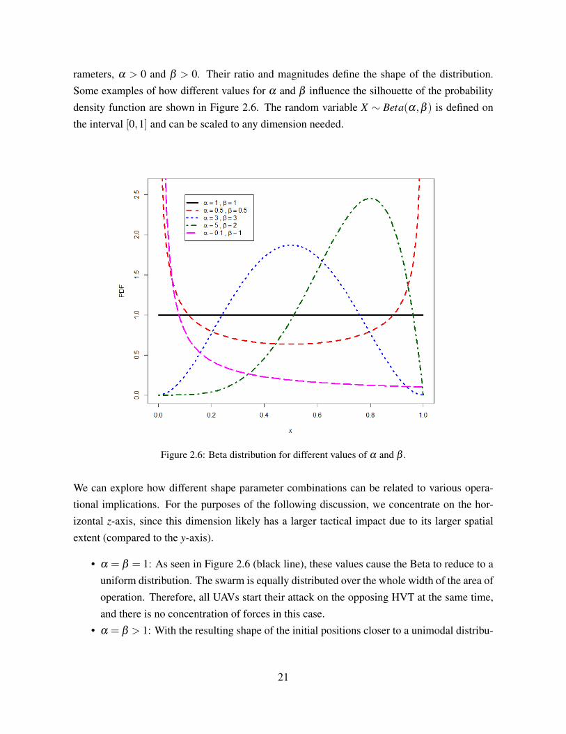
rameters, α > 0 and β > 0. Their ratio and magnitudes define the shape of the distribution.Some examples of how different values for α and β influence the silhouette of the probabilitydensity function are shown in Figure 2.6. The random variable X ∼ Beta(α,β ) is defined onthe interval [0,1] and can be scaled to any dimension needed.
Figure 2.6: Beta distribution for different values of α and β .
We can explore how different shape parameter combinations can be related to various opera-tional implications. For the purposes of the following discussion, we concentrate on the hor-izontal z-axis, since this dimension likely has a larger tactical impact due to its larger spatialextent (compared to the y-axis).
• α = β = 1: As seen in Figure 2.6 (black line), these values cause the Beta to reduce to auniform distribution. The swarm is equally distributed over the whole width of the area ofoperation. Therefore, all UAVs start their attack on the opposing HVT at the same time,and there is no concentration of forces in this case.
• α = β > 1: With the resulting shape of the initial positions closer to a unimodal distribu-
21

tion, the UAVs are more clustered about the home base. The amassed forces are thereforein the center and represent a more direct route (i.e., shorter distances) for the UAVs tofollow to the adversary’s home base.
• α < β or α > β : These values create a positively or negatively skewed distribution, whichputs the main effort on the left or right flank, respectively. The main force conducts a flankattack with maybe less resistance but longer distances to transit to the adversary’s homebase. This tactic could give an opponent that is attacking more directly down the centera time advantage. However, depending on the magnitude of the shape parameters, theremay be more or fewer defending UAVs remaining in the center and the alternate flank.These UAVs could be interpreted as a screening force that delays attacking enemies.
• α = β < 1: In this case, the forces are concentrated on both flanks (instead of retainingforces in the central area). This initial position might be advantageous for an adversarypredominantly in a defensive posture with its forces amassed centrally (i.e., not expectingattacks from the flanks).
The stated interpretation for parameter value combinations can be easily translated to the verti-cal axis (y-axis), where a beta distribution is also used.
2.2.3 Modeling of Individual AgentsWe next describe the behavior models for individual agents, the collection of which forms theswarm of UAVs. The individual agent is endowed with the ability to move, to recognize itsneighbors, to react to changes in the environment, and to coordinate its actions with some or allof its swarm teammates.
In this section, we describe the formal specification of the agent model which we implementin UAV.java. These mathematical models are implemented in sub models according to thedescription below. As a software implementation note, the step() method within each instanceof the UAV object is repeatedly executed by the simulation at each simulation time step in a event-based manner in order to run the behaviors of each agent, thereby executing all sub modelscontained within.
The breadth of the parameters that can be adjusted for each UAV object within the simulationsummarized in Table 2.1. The notation for the various parameters will be used in the descrip-tions and analysis throughout the remainder of this thesis.
22

Parameter Name Type Description Units
pE Position vector Position of the opposinghome base
hTE = (xpE ,ypE ,zpE )
pH Position vector The point in the space that theUAV tries to reach currently.
pTH = (xpH ,ypH ,zpH )
pP Position vector The position of the UAV atthe current simulation step
pTP = (xpP,ypP ,zpP)
V Directional vector Velocity vector
VT= (x
V,y
V,z
V)
vT Constant Cruising speed meters/second
vMin Constant Minimal speed meters/second
vMax Constant Maximum speed meters/second
vU p Constant Minimum speed a UAV canaccelerate to by climbing
meters/second
vDown Constant Maximum speed a UAV canaccelerate to by going down
meters/second
a Constant Acceleration factor meters/second2
aA Constant Acceleration factor for align-ment
meters/second2
aD Constant Acceleration factor for thecase where the UAV goesdown
meters/second2
b Constant Slowdown factor meters/second2
bA Constant Slowdown factor for align-ment
meters/second2
bU Constant Slowdown factor for the casewhere the UAV goes up
meters/second2
αMax Constant Maximum angular velocity degrees/second
s Constant Sensor range meter
w Constant Weapon range meter
k Constant Probability of kill meter
dMin Constant Minimum distance a UAVwants to maintain to all otherUAVs in the swarm
meters
continued on next page
23

continued from previous page
Parameter Name Type Description Units
dMax Decision Variable Is the radius of a spherearound the UAV. The UAVwants to stay close to allUAV of its swarm within thesphere.
meters
dc Constant Specifies a radius of a spherearound the center of mass.Where the center of mass isformed by all UAVs of theswarm within dMax.
meters
dH Decision Variable Distance in x direction atwhich the UAV starts toconverge to the opposinghome base (and therefore theswarm)
meters
nA Decision Variable Maximum number of alloca-tion per target
f Decision Variable Weight factor between mainobjective and other targets
Table 2.1: UAV parameter specification.
Motion Model for Bounded Curvature Flight
Given the assumption of fixed wing UAVs in the scenario, we note that a realistic model forthe flight dynamics of the vehicle should be addressed, as the vehicle must nominally remain inmotion to stay aloft. The flight dynamics of an airplane are dictated by the four forces: gravity,lift, thrust and drag. If we want to use this physical description, we would have to solve second-order differential equations, which would lead to a high computational effort, which opposes ourstated goal of generating insights without suffering the computational complexity and runtimeexpense. Therefore we make the decision to use a simplified geometry-based kinematic model,which does not consider the above forces but provides enough detail to reflect turn times andspatial movement.
24

This kinematic description of fixed wing aircraft, also known as describing vehicles with boundedcurvature, was first explained by Dubins [22] as part of a path planning problem in two-dimensional space and extended to three dimensions by Chitsaz et al. [23]. The vehicle de-scribed in the latter case is dubbed the Dubins’ airplane. However, [23] does not go far enoughfor our purposes, which require additional extensions to address the dynamic environment of ourswarm engagement scenario. Specifically, [23] assumed constant speed relative to the groundand decoupled changes in altitude as an independent degree of freedom. Rather, we combine allthree dimensions and introduce the velocity vector of the UAV, denoted
V , that does not have tobe constant throughout the UAV’s trajectory. Then the augmented state Q of an UAV in a singlesimulation step t is described by the current position pP and
V , that is,
Q =
xpP
ypP
zpP
V
With this definition of the velocity vector, one can identify a heading angle, which defines aheading at each time step towards a specific point in space, denoted pH . In general, given theobjective to reach and attack the adversary’s home base (located at pE), the heading is nominallyaligned in the direction of pE . However, we note that, based on the current mode of the UAV aswell as definition of the UAV behaviors, the desired heading could be towards other objectives.For example, for a given UAV agent, its pH could be the center of mass (COM) of the friendlyswarm, because the UAV has local preferences to stay close to its swarm teammates. pH couldalso be the current position of an opposing UAV because the UAV has some incentives to destroyit. As a result, given the dynamically changing environment, pH is never constant throughoutthe simulation run, and once pH changes, the UAV changes its direction and turns toward thenew pH .
In the following, we explain how the augmented state, Q, at the next simulation step, t +1, iscomputed. The directional vector
PH = pH − pp is defined as the vector which points from thecurrent position to the desired position. In order to turn an angle α between the two vectors
V and
PH has to be decreased by a certain amount. αmax is the maximum angular velocity theUAV is able to turn within one simulation step, and it is, therefore, the maximum angle α canbe decreased.
PH cannot be modified because the current position and the point of heading is
25

Figure 2.7: This is a rough picture of the idea of turning the velocity vector towards the vector definedby the current position and the point of heading.
fixed for this simulation step. But
V can be updated in a way that α is decreased. The mostchallenging part is to figure out in which direction
V should be turned, especially as we are in3D space. At the end the new position of the UAV pp is the point to which the updated velocity
vector
V is pointing (see Figure 2.7).
In order to compute the new UAV position pP and the new velocity vector
V we simplify the3D problem into a 2D problem.
V and
PH represent a plane in the space with normal vector
N =
V×
PH . If we consider
V as y-axis of the plane’s coordinate system given in 3D coordinatesthen
U =
V ×
N is perpendicular to
V and therefore the x-axis. Now we get the x-componentof the 2D representation of
PH by projecting
PH onto
U and taking the length of the resultingvector.
xPH
=
∣∣∣∣∣∣∣
U ·
PH∣∣∣U∣∣∣2
U
∣∣∣∣∣∣∣The y-component is the length of the projection of
PH onto
V .
yPH
=
∣∣∣∣∣∣∣
V ·
PH∣∣∣V ∣∣∣2
V
∣∣∣∣∣∣∣26

PH2D =
xPH
yPH
We also have to project
V onto
U and onto itself to get the 2D representation of
V . This issimpler because
V is one of the coordinate axes.
V 2D =
(0∣∣∣V ∣∣∣)
We want to calculate the smaller angle between
V 2D and
PH2D and the turn direction. Both aregiven by the equation
α = atan2(
yPH
,xPH
)−atan2
(x
V,y
V
)and the turn angle αT = sgn(α)max(|α| ,αmax) is used to compute pP. In this case we use theparametric equation of a circle in 3D because the new position of the UAV is somewhere on thecircle determined by pP as center and
∣∣∣V ∣∣∣ as radius.
V N and
UN are the normalized vectors of
V and
U respectively.
pP = pP +
V N cos(αT )∣∣∣V ∣∣∣+
UN sin(αT )∣∣∣V ∣∣∣
The updated velocity vector results from the difference between the new and the old position.
V = pP− pP
So far we do not have variability in the motion of a UAV as we see it in nature. Especiallyaircraft are affected by different air-streams, which makes it difficult to maintain a certain di-rection. We want to adjust the motion model to reflect this issue in the simulation. First we
define an arbitrary unity vector
WT= (0,0,1) that could be seen as the wind direction before
the current simulation step. The wind strength dW is a uniform random variable between zero
27

and 10% of the current velocity.
DW ∼U
0,
∣∣∣∣V ∣∣∣∣10
To determine the new wind direction we use the spherical coordinate system where the origin isthe current position pp of the UAV. The angles φ and θ are again two uniform random variables.
Θ∼U (0,2π)
Φ∼U(0,π)
They describe together with dW the new position of the UAV. But before we determine pp, weupdate the wind direction.
W =
∣∣∣∣W ∣∣∣∣ cos(θ)sin(ϕ)
sin(θ)sin(ϕ)cos(ϕ)
Then the new position is given by pp = pp +dW
W .
Modeling Climb and DescentAnother realistic issue is the impact of climbing or descending on the UAV’s velocity (whichis not addressed by Dubins’ airplane models in [23]). We want to reflect at least a part of thiseffect of trading between kinetic and potential energy in our model.
We assume the UAV should not stop completely (i.e., as in a stall), and so introduce the mini-mum speed, vU p. We also define vDown as the maximum speed an UAV can reach as it descends.In the right-handed coordinate system, the y-axis determines the altitude of a given UAV andy
Vshows the change in altitude in the current simulation step.
In the case yV> 0 the UAV climbs and is assumed to decelerate by a factor bU < 1 only if
the current velocity exceeds the product of vU p and the ratio of the current velocity and itsy-component.
28

V =
bU
V ,∣∣∣V ∣∣∣> vU p
( ∣∣∣V ∣∣∣y
V
)
V ,∣∣∣V ∣∣∣≤ vU p
( ∣∣∣V ∣∣∣y
V
)
In the worst case yV=∣∣∣V ∣∣∣ the UAV decelerates to vU p. If the change in altitude is not so
aggressive, then the UAV decelerates to a velocity between vU p and
V . This takes into accountthat a higher speed can be maintained for a lower climb rate.
The same works for yV< 0 respectively, where aD > 1 is the acceleration factor.
V =
aD
V ,∣∣∣V ∣∣∣< vDown
∣∣∣yV
∣∣∣∣∣∣V ∣∣∣
V ,∣∣∣V ∣∣∣≥ vDown
∣∣∣yV
∣∣∣∣∣∣V ∣∣∣Parametrized Sensor Model
We assume that the UAV is equipped with a hemispherical cookie-cutter sensor with sensorrange s. In other words, the UAV is able to detect every opponent UAV in its front hemispherewithin s.
Algorithmically, the relationship between all UAVs in the space is initially stored in an undi-rected network, denoted Ψ, where every UAV has an edge to every opponent UAV. Based onthis data structure, UAV i has now access to every hostile UAV j and can measure the distances j, for each i. If s j is smaller than s for a given i, then an edge is drawn in a second directednetwork, denoted Γ, from node i to node j. This procedure assumes perfect identification offriend or foe. This method enables tracking of simulated detections amongst all UAVs of theiropponents at each time step. Note that these detections are cleared at the beginning of everysimulation step, and the procedure starts over. Further, we assume that all UAVs have instan-taneous access to the collective set of detections taken by all swarm teammates because of theassumption of perfect communication among teammates.
29

2.2.4 UAV Swarm ModelingHaving adequately described the individual UAV agent models, we can begin to describe theswarm behaviors emerging from the collective local rule sets and the interactions among theindividual agents. An assumption of the swarm is the ability for all UAVs to know their ownpositions and that of their teammates (or a subset thereof), made possible through the use ofbroadcast communications among the swarm. As will be described further in this section, eachsingle UAV is now able to determine its relative position in the swarm and take actions to getcloser, increase separation, and/or adapt speed and direction relative to its neighbors. Anotheradvantage of this perfect communications assumption is the opportunity to allocate targets inan optimized way among the swarm elements, which we leverage in this work to present adecentralized solution.
Flocking Behaviors: Cohesion, Separation, AlignmentCraig Reynolds identified three key behavior patterns in his paper [6] for generating flockingbehaviors: cohesion, separation and alignment. Their implementation is often termed “boids al-gorithm.” In this section, we describe how we adapt Reynolds’ idea to the proposed swarm UAVmodel by first describing these three relevant behaviors and their modified implementations inthis work.
• Cohesion: Recall that the UAVs within a swarm possess a complete communication net-work to interact with each other. This network is represented by the two undirected net-works ΩB (for the Blue swarm) or ΩR (for the Red swarm) where every UAV has a linkto every friendly UAV. An arbitrary UAV at position pPi is aware of all positions pPj of allother UAVs j in the swarm. The sum of the positions divided by the number of teammateUAVs n−1, not including itself, gives the center of mass (COM), denoted c, for UAV i.
c =1
n−1
n
∑j=1; j 6=i
pPj
We define dc as the radius that specifies a sphere around c. One desire of a UAV is to stayin this sphere close by its swarm members. But c will certainly move towards pE overtime. Therefore the UAV makes a prediction and updates its desired heading target point,pH , according to:
pH =12(pH− c)
Recall that the UAV has a cruising speed vT , a minimum speed vMin and a maximum
30

speed vMax. In the case where the UAV is in front of c it decelerates by factor b < 1 until∣∣∣V ∣∣∣ reaches vMin. If the UAV is behind the swarm then it accelerates by factor a > 1 until∣∣∣V ∣∣∣ reaches vMax. The UAV slows down or accelerates by b and a, respectively, until∣∣∣V ∣∣∣
reaches vT to achieve this cohesive behavior.• Separation: The next step is to ensure that UAV i stays away a distance dMin from its
neighbors. First, each UAV identifies the closest UAV j and measures the distance, d j.If d j is smaller than dMin then it turns
PH a certain angle βT away from the vector
Pi j =
pPj − pp. This is done in the same way as described in the motion section above, suchthat the updated target heading point is given by:
pH = pH +
PHN cos(βT )
∣∣∣∣PH
∣∣∣∣+
UN sin(βT )
∣∣∣∣PH
∣∣∣∣• Alignment: All UAVs follow one commonly known global goal, which is to target (and
nominally destroy) the opposing home base located at position pE . The UAVs always tryto fly towards this point. Therefore, for the given swarm agents, we do not specificallyneed to address alignment behaviors because as long as the UAVs follow the global goal,they more or less line up automatically.
Target Allocation Optimization ModelIn addition to motion control, we need a mechanism that assigns friendly UAVs to appropriateenemy UAV to engage and defeat, which is based on relative positions in terms of range to thetarget and relative bearing, γi j, as measured as the angle between
V i and
Pi j, the latter of whichis the vector from agent i to enemy UAV j. The goal of the presented algorithm is to constructa decentralized approach to the allocation model. We note that the presented heuristic algo-rithm, iterated at every time step, provides a sub-optimal decentralized solution. A centralizedmethod would leverage a network optimization algorithm that can provide optimal assignments;however, the decentralized architecture provides both robustness to a single point-of-failure aswell as addresses the dynamically changing network topology in an efficient manner. For com-parison of assignment performances, the centralized allocation is formulated and solved usingnumerical optimization software (i.e., General Algebraic Modeling System [?]). The resultsshow that the objective value of the decentralized method is, on average, 20% above the opti-mal cost. This performance gap is deemed acceptable, given the advantages provided by thedecentralized architecture, e.g., individual UAVs can optimize their allocations locally.
UAV i can use the appropriate network data structure, ΩB or ΩR, to identify all friendly UAVs
31

in its network, Γ, and therefore have access to positions of all detected enemy UAVs j currentlyin the collective field of view of the friendly swarm. Another directed network Λ keeps track ofall currently allocated targets. Let m j be the number of allocations for UAV j, and let
∣∣∣Pi j
∣∣∣ bethe distance between UAV i and j. Further, define f as the weight factor between the primaryobjective (i.e., targeting the adversary’s home base) and other targets (i.e., targeting enemyUAVs). In other words, f represents the preference of the UAV to engage in an offensive role( f large) or a defensive role ( f → 0). Then the expression below
gi j =(m j + f
)(∣∣∣Pi j
∣∣∣+ γi j
αMax
∣∣∣V i
∣∣∣)defines the desired objective function with a penalty for multiple allocations, m j, for the sametarget. The main idea is that we want multiple allocations to ensure redundancy (i.e., highprobability of kill for a given target) but not too many friendly UAVs allocated to one target toavoid the possibility of untargeted enemy UAVs.
In order to address the dynamically changing environment (since the enemy UAVs are alsomaneuvering in offensive and defensive roles), we also enable adaptive target allocations. Todo so, define gMin, which identifies the target currently with the lowest objective value, where|pE − pP| represents the distance to the adversary’s home base:
gMini = min(∣∣pE − ppi
∣∣ ,gi1,gi2, . . . ,gin)
The UAV j corresponding to gMini is considered a priority target, and an edge is drawn in Λ
from i to j. However, given the operational constraint that limits the number of allocations pertarget, define this maximum number of friendly UAVs to target a single enemy UAV as nA. Inthe special case where f
(∣∣∣Pi j
∣∣∣+ γi jαMax
V i
)≤∣∣pE − pp
∣∣ and m j = nA, UAV i tries to find one
friendly UAV l that allocates UAV j with(∣∣∣Pi j
∣∣∣+ γi jαMax
V i
)<(∣∣∣Pl j
∣∣∣+ γl jαMax
V l
). Then UAV
i deletes the allocation and allocates UAV j itself. In other words, target allocations can betraded among teammates if more (locally) favorable allocations are available. Finally, note thatthe target allocations for all UAVs are reset and recomputed at the beginning of every simulationstep. This adaptive approach ensures the latest common operational picture is used to generatethe target allocations. However, such a myopic approach may be limited due to its potential
32

sub-optimality over many time steps; study of improved methods is left for future work.
Once a UAV is given an allocation of a particular target, the UAV mode transitions to combatmode, and no longer adheres to the local behaviors of cohesion and separation. Other swarmmembers also exclude this UAV from further consideration that concern collective swarm mo-tions. According to Day [8], UAV speed can be seen as a significant factor in UAV-versus-UAVcombat. Therefore, when in combat mode and attempting to shoot down an enemy UAV, theUAV will accelerate up to vMax in order to gain any tactical advantage possible. Additionalcharacteristics of this combat mode are described in the following section.
2.2.5 Combat modelWe assume that the UAV is equipped with a cookie cutter weapon that is pointing in the directionof
V (i.e., relative to the nose of the UAV), and is able to hit the target within a range w withprobability k. The weapons range, w, is assumed smaller than sensor range, s. The UAV i
attacks the allocated target and tries to reduce the relative bearing angle, ωi j, to the target j. ωi j
is the angle between
V i and
Pi j. As soon as ωi j < 45/∣∣∣∣Pi j
∣∣∣∣, and the range to the target is less
than w, the UAV shoots at the target. The probability of kill is determined by k and the exposed
surface area of target which depends on the angle ρi j between
Pi j and
V j. For that we see thetarget as a point and divide the anticipated sphere around the point in eight equal sectors. Eachsector has an opening angle of 90 degrees and is associated with the front, rear, top, bottom, leftor right side of the target. ρi j determines the sector and therefore the exposed area At . Then theactual kill probability is computed by
π = kAs
maxs(As); s ∈ 1,2,3
Therefore an attacker has an higher chance to kill a target if it is attacking from below or above.We see the impact of this benefit related to the initial positioning. For example, a swarm thatstarts almost at the maximum ceiling, the main force attacks more likely from above and getsthe tactical advantage, at least in the early phase of the combat. With this implementation, wehope to see configurations that exploit such considerations.
2.3 Markovian ModelThis section outlines an analytical model to provide aligned but alternate insights about swarmtactics studied in this thesis. This stochastic process model describes the swarm engagement
33

scenario from a different point of view, and sensitivity analysis gives additional informationabout the consistency of the simulation results described previously.
We define a Markov process to explore the scenario in a mathematically rigorous manner. Thepresented approach explores two levels of abstraction. The first one deals with the one-on-onecombat situation, whereas the second model applies the results of the first level to the multi-UAVscenario developed later on in this section. The decomposition into these two levels essentiallytakes out the individual dog fighting elements from the multi-UAV engagement. Studying bothsub models provides more insights and allows for more tractable analyses. For each of thesemodels, we are interested in the long term behavior of the Markov process, with absorbing statesrepresenting victory conditions for either Blue or Red swarms.
2.3.1 One-versus-One CombatThis model can be thought of as the engagement scenario that has only one UAV and the HVTon both sides. The UAVs start in a state in which they are not yet engaged in combat. There issome chance that an engagement (i.e., a dogfight) will ensue, in which one UAV shoots downthe other or one UAV destroys the opposing HVT before it itself is defeated.
The following states describe the possible situation in such a scenario. Given that we do notconsider fuel or ammunition shortages, there are no draw states; in other words, all end statesdictate a clear win situation for one side or the other.
• State 0 (transient): Both UAVs start in this state. There is no combat at the beginning.This can also be envisioned to be the search phase where both try to detect the opposingUAV or fly against the adversary’s HVT. Also, during an ongoing dogfight, there is somepossibility that the evader is able to escape, at which point both UAVs return to this state0.
• State BvR (transient): Blue detects Red with some probability and manages to get in apursuing position, or Blue was originally pursued by Red but has turned the table on Red.In this case, Blue has the tactical advantage and can try to kill Red.
• State B (absorbing): Blue pursued Red and shot Red down. The engagement is over andBlue won (since there is only one UAV on a side).
• State RvB (transient): Red detects blue with some probability and manages to get in apursuing position, or red was originally pursued by blue and turned the table on blue. Inthis case, red has the tactical advantage and can try to down blue.
34

• State R (absorbing): Red pursued blue and shot blue down. The engagement is over andred won.
• State HVTR (absorbing): Blue reached red’s HVT and destroyed it. This can happen evenif Blue was previously engaged in a dogfight. Either red pursued blue and was not ableto stop blue before it reached red’s HVT, or blue attacked red and they came sufficientlyclose to red’s HVT that blue had a higher reward to attack red’s HVT than maintaining itspursuit of the Red UAV. In this case, Blue completed the mission and won.
• State HVTB (absorbing): Red reached blue’s HVT and destroyed it. Red won in this case.
The state diagram for one-on-one combat is shown in Figure 2.8. Blue and red are together inone of the transient states 0, RvB or BvR as long the scenario continues. As soon as one UAVenters one of the absorbing states, that is, B, R, HVTR or HVTB, the engagement is over and thecorresponding party wins.
Figure 2.8: State diagram for the one-on-one combat (level 1).
For this state transition model, probabilities can be prescribed that govern the transition fromone state to another, such that pi, j now represents the probability of transitioning from state i tostate j. The transition probability matrix can be written in canonical form, given by(
I 0R Q
)
35

where R gives the transition from a transient state to an absorbing state and Q represents the tran-sitions among the transient states. Table 2.3.1 thus is the matrix representation in this canonicalform of the Markov process illustrated in Figure 2.8.
B R HVTR HVTB 0 BvR RvBB 1 0
0R 1HVTR 0 1HVTB 1
0 0 0 p0,HR p0,HB 0 p0,B p0,RBvR pB 0 pB,HR pB,HB pB,0 0 pB,RRvB 0 pR pR,HR pR,HB pR,0 pR,B 0
Table 2.2: One-step transition probability matrix for level one (one-on-one combat)
Given this canonical form, the steady-state transition probabilities from the transient states tothe absorbing states can readily be computed by the matrix equation, as referenced in Ross [24]:
B = (I−Q)−1R (2.1)
Since the engagement always starts in state 0, we are only interested in the transition probabili-ties from this state into the absorbing states, summarized by the following matrix:
B1 =
p10,B p1
0,R p10,HR p1
0,HB
p1B,B p1
B,R p1B,HR p1
B,HB
p1R,B p1
R,R p1R,HR p1
R,HB
These transition probabilities represent the starting point for the second level model, movingbeyond one-on-one combat and describing multi-UAV engagements.
2.3.2 Multi-UAV EngagementTo study swarm engagements, we want to increase the numbers of UAVs on each side to 50 asdescribed in the original reference scenario. In order to do so, we assume that only one eventhappens at a distinct point in time. This is either the defeat of a UAV or the destruction ofan HVT. The results from the previous section determine the probability at which each eventoccurs. A UAV gets shot down with probability p1
0,B or p10,R, and an HVT is taken out of action
with probability p10,HR or p1
0,HB.
36

The transient states for this Markov process are represented by the available UAVs on bothsides. The state 50/50 is the starting point where 50 blue UAVs and 50 red UAVs are in thebattle arena. In this naming convention, the first number always reflects the number of blueUAVs and the second number counts the red UAVs. Starting with 50/50, the stochastic processeither goes to 50/49 with probability p1
0,B or to 49/50 with probability p10,HB. This process goes
on until one side reaches zero. All states where one party has zero UAVs left is an absorbingstate. In every transient state, there is also some probability that one of the HVTs get destroyed,in which case, the engagement is determined, and the party who destroyed the HVT won. Foran illustrate of this multi-UAV engagement Markov model, see Figure 2.9.
Figure 2.9: State diagram for level two (multi-UAV engagement).
As before, we wish to study the long term behavior of such a multi-UAV engagement. We onceagain use the canonical form of the transition probability matrix as before (see Equation 2.1).Then the relevant transition probabilities for this second level model are summarized by B2:
37

B2 =
p2
50,50/0 · · · p250,1/0 p2
50,0/1 · · · p250,0/50 p2
50,HR p250,HB
......
......
......
p21,50/0 · · · p2
1,1/0 p21,0/1 · · · p2
1,0/50 p21,HR p2
1,HB
,
which determines the long term transition probabilities from any transient state into all absorb-ing states. Since the scenario starts always with 50 blue against 50 red UAVs, the first row of B2
gives the probabilities for the different end states. For completeness, the full transition matrixcorresponding to this Markov model is thus given in Table 2.3.2.
50/0 49/0 · · · 1/0 0/1 · · · 0/50 HVTR HVTB 50/50 50/49 · · · 49/50 49/49 · · · 1/150/0 1
0
0
49/0 1...
. . .1/0 10/1
0
1...
. . .0/50 1
HVTR 1HVTB 150/50 0 0 · · · 0 0 · · · 0 p1
0,HR p10,HB 0 p1
0,B · · · p10,R 0 · · · 0
50/49 0 0 · · · 0 0 · · · 0 p10,HR p1
0,HB 0 0 · · · 0 p10,R · · · 0
......
......
......
......
......
......
...49/50 0 0 · · · 0 0 · · · 0 p1
0,HR p10,HB 0 0 · · · 0 p1
0,B · · · 049/49 0 0 · · · 0 0 · · · 0 p1
0,HR p10,HB 0 0 · · · 0 0 · · · 0
......
......
......
......
......
......
...1/1 0 0 · · · p1
0,B p10,R · · · 0 p1
0,HR p10,HB 0 0 · · · 0 0 · · · 0
Table 2.3: One-step transition probability matrix for level two (multi-UAV engagement).
Given this theoretical model formulation, further analysis in Chapter 4 will outline how wechange some of the probabilities in the level one model and observe its impact on steady stateprobabilities in the second level model. The sensitivity analysis should disclose critical parts inthe scenario and enable recommendations for systems in such an environment.
38

CHAPTER 3:
Design of Experiments
After having defined and developed the two complementary models for exploring the swarm-versus-swarm scenario, we now want to use these models to gain insights regarding swarmtactics in swarm combat engagements. In particular, we design simulation experiments for theconstructed simulation model, using two different experimental designs to address the com-plexities of the model. The objective of the experimental design described in this chapter is todiscover and characterize the influential variables and their interactions. Knowledge of thesesignificant factors directly guides the rigorous statistical analysis conducted in Chapter 4, inwhich we delve more deeply into the results of the simulation experiments, and also re-connectthose results with the Markov process stochastic modeling effort.
In terms of the applied scenario, swarm combat could potentially be broken down into mul-tiple one-on-one fights. In this case, parameters such as speed, maneuverability, or weaponcapabilities would be decisive. However, the purpose of the present study is to specifically in-vestigate the implications of swarming with large numbers of UAVs on each side. We reiteratethis emphasis as the reason for assuming technological parity by using the same type of UAVon both sides. In this context, a dogfight between two singular UAVs would always be unde-termined since both are equally matched. Instead, other tactical factors like initial positioning,offense-defense preferences, or swarm behavior may influence the simulation outcome, andtheir illumination is the focus of this thesis.
During the development phase of the simulation model, we incorporated a preliminary intuitionon the nature of the swarm engagement scenario by identifying many design parameters relevantto the scenario and combat environment, the individual agent motion and sensing rules, and thecollective swarm behaviors. In this chapter, we more formally describe the variables of interestand describe the produced simulation output. We then outline and generate various statisticalexperimental designs, which help to screen for important regressors and interactions betweenthe defined input variables. Having also defined the appropriate response variables, namelythe measures of effectiveness including the probability that Blue wins the engagement and thesurviving force strengths of Blue and Red UAVs, the simulation experiments themselves andrelevant quantities are described in further detail.
39

3.1 Variables of InterestBased on preliminary assessment of the simulation, we identify twelve key variables whichseem to influence the responses. These variables and their nominal ranges are provided inTable 3.1, with more detailed description of each of the relevant factors given thereafter.
Variable Name RangeX1 NumAllocBlue [1, 9]X2 NumAllocRed [1, 9]X3 CohesionMax [500, 10000]X4 ConvergeBlue [500, 10000]X5 ConvergeRed [500,10000]X6 WeightBlue [0, 10]X7 WeightRed [0, 10]X8 StayingPwHVT [1, 11]X9 YAlpha [1, 1001]X10 YBeta [1, 1001]X11 ZAlpha [1, 1001]X12 ZBeta [1, 1001]
Table 3.1: Simulation variables considered in the presented statistical design of experiments. Each ofthese factors are systematically varied over the defined ranges during several simulation replications.1
NumAllocBlue and NumAllocRed are the maximum numbers of possible allocations of friendlyUAVs to a single detected (enemy) target. The number of allocations ranges from one to nine.This range seems reasonable since we have to allow at least one allocation and even if ten allo-cations are possible, this number will likely rarely be observed because of the penalty functionfor target allocation explained in Section 2.2.4. However, given the possibility that there areisolated situations where a whole swarm on one side meets just a few opposing UAVs, this highfactor level may identify interesting results. In general, we can think about this variable as ameasurement of force concentration at the engagement level. A higher value will concentratethe fire on few enemies with a higher survival rate for the friendly force.
CohesionMax determines the distance relative to a given UAV within which it includes swarmmembers in its calculation for the center of mass. This parameter influences the individualUAV’s behavior for cohesion, which guides the collective motion, and gives an idea of howclose the cohesion within the swarm is. The range goes from 500 meters to 10000 meters,
1The ranges are adjusted (e.g., upper levels at 9, 11 or 1001, instead of 10 and 1000, respectively) such that thecenter values within the interval are integers (e.g., 5, 6 and 500, vice 4.5, 5.5, and 500.5).
40

where the swarm is loosely assembled for lower values and transits in more tightly arrangedconfigurations for higher values.
ConvergeBlue and ConvergeRed define the distance to the respective adversary’s HVT atwhich the swarm UAVs converge to attack the HVT directly. A small value of 500 metersmeans that the swarm uses the whole width of the battle space to approach the area where theopposing HVT is located and attack it from three sides. In the case where the enemy sends itsUAVs straight through the middle, employing a short convergence range might allow friendlyUAVs to reach the HVT without many engagements. This would amount to a tactic known asa flank attack. The trade-off in this scenario is that both sides have the same number of UAVs.Therefore, if executing a flank attack, then the center is nearly undefended against an enemy’sconcentrated force down the middle, and approaching from the flanks results in a longer path tothe HVT. Alternatively, for example, with a high value of 10000 meters for this parameter, theswarm would start their attack directly at the beginning and nominally concentrate their forcein the center. This could mean that some opposing UAVs could reach the rear area undiscov-ered behind the advancing friendly swarm while the swarm is forced into dogfights with theadversary’s main force and delayed from striking the adversary’s HVT.
WeightBlue and WeightRed determine the weight factor f in the penalty function introducedin Section 2.2.4. In general, this value defines whether a swarm is more or less defensive oroffensive. A low value of zero leads to a lack of preference between attacking the adversary’sHVT and attacking a detected enemy UAV, with the friendly UAV attacking whichever is op-portunistically closer. In this case, if the two swarms meet in the open battle space, the distanceto every opposing UAV is smaller than to the opposing HVT. Therefore, a UAV always attacksdetected targets and tries to prevent them from attacking its own HVT. We see this as a defen-sive posture. As the value of f increases, the preference of the UAV to attack the HVT getsstronger. With a value of 10, the UAV no longer cares about engaging any enemy UAVs butrather is focused on attacking the HVT. We can interpret this as offensive behavior. Let us lookat a simple arithmetic example. Suppose the weight factor is nine. The battle space has a di-mension of ten by ten kilometers. Therefore, the distance from the UAV to the opposing HVT isabout ten kilometers at the beginning. Both swarms meet approximately in the middle. So, thedistance to the HVT is approximately six kilometers. A target is detected 0.7 kilometers away.But 0.7 ·9 > 6 and the UAV ignores the detected target.
41

StayingPwHVT defines the number of hits needed in order to take an HVT out of action. Thisvalue was originally not supposed to be a variable for this analysis. Early simulation runsshowed that it is easy for a swarm to have at least one successful UAV strike on the HVT. How-ever, this result in isolation does not mean that the swarm necessarily has a tactical advantage.It is also more realistic to assume that an HVT is able to resist more than one attack, eitherthrough design or by self-defense capabilities.
YAlpha, YBeta, ZAlpha and ZBeta are the input parameters for the two Beta distributionswhich generate the initial positioning for the Blue swarm. We want to explore if the initialspatial configuration of the swarm makes a difference in the outcome of a battle while the ad-versary swarm is always uniformly distributed. Rather than defining fixed setups, we would liketo screen over all possible initial positions. The two-parameter Beta distribution is one option toachieve this goal. There are two main advantages of this distribution. First, it always producesrandom numbers between zero and one, which can easily be scaled to the dimensions of thebattle space. Second, varying the input parameters, α and β , structurally changes the outputdistribution, spanning from the uniform to unimodal to left- and right-skewed distributions. Ifwe do so and vary the four input parameters (two each for y- and z-axes), we see spatial con-figurations that are (a) almost equally distributed over the whole space, (b) more centered, (c)more concentrated on the left, right or (d) on both flanks, and analogously with changes in thealtitude. Figure 3.1 shows how the input parameters influence the positioning. The prescribedranges for these parameters is [1,1001]. Note that this interval is only for convenience while wegenerate the design, as the simulation divides each value by 100, such that the effective rangethat the simulation uses is [0.01,10.01].
3.2 Generation of the Design of ExperimentsThe goal is to explore the above mentioned factors and their two- and three-way interactionswith respect to their influence on the simulation output. We also must check for non-linearityand, if necessary, adapt the model subsequently in the analysis. One widely used approach indesign of experiments (DoE) are factorial designs (see [25]) where every factor is observed at itslow and high levels, and possibly one or more levels in between. These designs are orthogonal,which results in no correlation between all the main effects and their interactions. They alsoprovide the ability to explore all possible interactions. The biggest drawback is the high numberof design points that have to be run. In our study, we have twelve factors, and we recognize theneed for at least three levels per factor because we want to observe any nonlinear effects. Such a
42

Figure 3.1: Illustrations of various Blue UAV swarm initial position configurations while varying theannotated input parameters for the beta distribution in y- and z-directions, yielding (a) a more centralizedsetup in a higher position, (b) a force concentration on both flanks, and (c) a uniform distribution in thewidth and centralization in the height.
design would lead to 312 = 531441 design points. Let us say we run every design point with 30replications, which now results in 15,943,230 total replications. Given that a single run takesabout four seconds on an up-to-date computer, we would need about two years to complete theexperiment. This is not acceptable.
An alternative to factorial designs are fractional factorial designs. These designs assume thathigher order terms are essentially negligible. The resolution of such a design explains the wayin which the observed effects are confounded with each other. For example, a resolution-III
43

fractional factorial design ensures that the main effects are not confounded with each other;however, they may be confounded with two-way interactions or other higher-order terms. Ifwe were to use such a design, we would be restricted to the main effects only, and would beforced to assume that higher-order terms are noise that do not influence the model significantly.Given the variability and complexity of the model, we wish neither to make this assumption norto discard potentially meaningful influences. According to the stated goal above, a resolution-VII fractional factorial design appears to be a satisfactory choice: The main effects includeonly the noise from the sixth-order terms or higher, the second-order terms only from the fifth-order terms or higher, and the third-order terms from the fourth-order terms or higher. In otherwords, we assume that the fourth-order terms and higher are not significant for our model. For afurther discussion of fractional factorial designs, we refer the reader to Sanchez [25] or Kleijnenet al. [26]. Draper and Lin [27] state that a resolution-VII fractional factorial design for twelvefactors (215−5
V II ) would comprise 210 design points. If we repeat the calculation as above, thenwe need only 30,720 runs. This is approximately equivalent to one and a half days, and if wewere to take advantage of multi-core processing, then we could decrease this to an overnightrun, which is more appropriate for our purposes.
However, this choice of design would not completely achieve the designated goal, since thefractional factorial designs observe only two levels of each factor. This high-low setup wouldbe enough for a linear regression model, but we would not be able to see any nonlinear effectsif some are present. However, a center composite design (CCD) is one that we can use toobserve non-linearity in the model [25]. We take the 215−5
V II design and add center point andstar-points for every factor. A star point varies only one factor at a time. All other factors arekept at the center of the range. Therefore, we see two star points for every factor (one for thelow and one for the high value). The resulting design contains 1050 design points and givesus the opportunity to fit a model with three-way interactions and to observe nonlinear effects.Sanchez [28] provides a solution to generate such a design effectively (see Table 3.2), wherethe factors, X1, . . . ,X12 are the variables in the same order as explained in Section 3.1 (also referto Table 3.1).
As we will see in later analysis, there are non-linear effects among the factors. So we did well bychoosing a design that is able to detect such effects. However, with only three observed levels,we cannot fully explore the real nature of these effects and not all are necessarily quadratic. Wewould need more observations in between at intermediate levels. A Latin hypercube design isuseful in this case because of the space-filling properties and the relatively few design points
44

n X1 X2 X3 X4 X5 X6 X7 X8 X9 X10 X11 X121 1 1 500 500 500 0 0 1 1 1 1 12 9 1 500 500 500 0 10 1 1 1 1001 13 1 9 500 500 500 0 10 1 1 1 1001 14 9 9 500 500 500 0 0 1 1 1 1 15 1 1 10000 500 500 0 10 1 1 1 1001 1...
......
......
......
......
......
......
531 1 9 500 500 10000 0 0 1 1 1 1001 1001532 9 9 500 500 10000 0 10 1 1 1 1 1001533 1 1 10000 500 10000 0 0 1 1 1 1001 1001
......
......
......
......
......
......
...1023 1 9 10000 10000 10000 10 10 11 1001 1001 1001 10011024 9 9 10000 10000 10000 10 0 11 1001 1001 1 10011025 5 5 5250 5250 5250 5 5 6 501 501 501 501
......
......
......
......
......
......
...1048 5 5 5250 5250 5250 5 5 6 501 501 1 5011049 5 5 5250 5250 5250 5 5 6 501 501 501 10011050 5 5 5250 5250 5250 5 5 6 501 501 501 1
Table 3.2: Resolution VII fractional factorial design with star and center points for 12 factors. X1 to X12refer to the variable names in Table 3.1. There are 1050 design points overall. 2
needed. Sanchez provides a spreadsheet tool that generates Nearly Orthogonal Latin Hypercube(NOLH) designs for up to 29 factors [29]. This tool satisfies our need for 12 factors, and theresulting NOLH design comprises 65 design points. This design is shown in Table 3.3.
3.3 Simulation Response VariablesIn the sections above, we outline and design the input parameters for the simulation model. Wenow turn to the simulation output, which represent the measures of effectiveness or responsevariables that we analyze in the next chapter to make recommendations for successful swarmbehaviors and generation of swarm tactics. As they will be addressed in thorough detail, wesimply state and briefly describe each of the simulation outputs here.
BlueWon is a binary variable that is zero if Red was successful in a particular simulation run, andone if Blue accomplished the mission, as defined by destroying the adversary’s HVT. Severalruns are be conducted for each design point. The average of this response variable, BlueWon,
2The complete design matrix in comma-separated value format (filename DoE_CCD.csv) can be downloadedfrom http://faculty.nps.edu/thchung under Software.
45

n X1 X2 X3 X4 X5 X6 X7 X8 X9 X10 X11 X121 7 1 3914 3617 1688 8 8 5 969 719 547 9382 10 7 1539 4508 3766 3 5 8 719 922 766 4853 9 4 9555 2578 3320 9 2 5 407 579 797 8754 7 9 7328 4805 1094 4 3 3 126 984 906 6255 9 5 2281 648 1391 2 3 6 610 485 63 844...
......
......
......
......
......
......
61 2 2 4063 2133 1242 7 9 4 266 641 625 1762 2 7 8813 4211 3914 8 6 9 781 141 126 45463 4 2 6734 3023 1539 0 7 5 938 220 391 32964 4 9 3320 4656 945 6 2 3 79 32 188 46965 2 4 1094 1836 3172 4 1 4 344 391 173 235
Table 3.3: Nearly Orthogonal Latin Hypercube design for 12 factors. X1 to X12 refer to the variablenames in Table 3.1. There are 65 design points overall. 3
for a particular set of runs gives the probability for an expected Blue success for a particulardesign point. Higher probabilities identify better configurations for the Blue swarm and indicatepotentially relevant swarm tactics considerations.
SurvRed is the number of Red survivors. Even if Blue accomplished the mission and destroyedthe Red home base, Red could have more UAVs remaining than Blue. These enemy UAVswould nominally continue to pose a threat on Blue’s home base. This fact should also be takeninto consideration when developing simulation configurations. This output is also a startingpoint for further development of the simulation model to modify the termination criterion formultiple HVTs or extended engagements.
SurvBlue is the number of Blue survivors. The same statements above hold for this measure.We could combine SurvRed and SurvBlue as a force ratio and incorporate this ratio into theanalysis as a single response variable.
DistanceCenter and DistanceUAV are not explicitly MOEs; however, these variables aregenerated by the simulation and are closely connected to YAlpha, YBeta, ZAlpha and ZBeta
parameters. Though the α and β values for the beta distributions in y- and z-axis initial positionshave no directly operational meaning, we can transform these parameters into measurementsthat can be taken in operational contexts which express the initial positioning of swarm quitewell. DistanceCenter gives the distance from the center of the bin where the Blue swarm
3The complete design matrix in comma-separated value format (filename DoE_NOLH.csv) can be downloadedfrom http://faculty.nps.edu/thchung under Software.
46

is initially staged to the COM of the entire swarm. This value gives an idea of how the mainforce of the swarm is situated with respect to the HVT, recalling that the center of the binis directly above the HVT. DistanceUAV is the average distance of the UAVs to the COMof the swarm. The higher the value, the more dispersed the swarm is initially. Figure 3.2illustrates this visually. Rather than using the α and β values as regressors in the simulationanalysis, we choose to analyze the more operationally grounded responses of DistanceCenterand DistanceUAV.
Figure 3.2: Schematic diagram for the measurement of response variables, DistanceCenter and Dis-tanceUAV. “Center” is the center of the bin where the Blue swarm is positioned initially. “COM” isthe center of mass of the swarm. DistanceCenter is the gray line that describes the distance between“Center” and “COM.” DistanceUAV is the average distance of all UAVs to the COM (symbolized bythe blue line).
3.4 Conducting the ExperimentWe wish to run the simulation with the generated designs. Before we can begin execution, wemust find the appropriate number of replications for each design point to achieve the statisticalpower we require. A power calculation can help here and is essentially an inverted hypothesistest where we specify the sensitivity level and the probabilities for Type I and Type II errors atthis specified level. Let us state the hypothesis first.
H0 : pBlueWon = 0.5
Ha : pBlueWon 6= 0.5
The null hypothesis is that Blue has a 50% chance to win for every given design point. Thealternative is that Blue’s probability of a success is lower or higher than 50%. So, this is a
47

two-sided test. Remember that we use a central composite design which enables screening forimportant factors. Though it will not capture or explain the whole model, we consider this initialexploration as acceptable as we conduct this preliminary analysis to obtain some early insights.We should account for this preliminary nature in our determination of an appropriate number ofreplications. In our study, the Pareto principle can be applied to this case, which says that wecan explain 80% of the model behavior with 20% of the effort (as measured by the number ofsimulation runs in this case) that we would need to explain 100% of the model. We can set theprobabilities for Type I and II error according to this principle. We reject H0 with a maximalerror of α = 0.2 (Type I error) and fail to reject if Ha is true with β = 0.2 (Type II error) ata sensitivity level of 0.1. As this is a two-sided test, a sensitivity level of 0.1 is equivalent toan interval of 20% centered about the mean. The number of replications that gives the desiredpower is determined by:
n =
(σ(zα/2 + zβ )
(pa− p0)
)2
,
where (pa− p0) defines the sensitivity level, denoted d. For those who are interested in adeeper discussion about this part, we recommend Wackerly, Mendenhall and Scheaffer [30].As we do not know the true standard deviation σ of the population, we can estimate it byrunning the simulation with an appropriate initial number of replications. The presented NOLHdesign is a good choice for this purpose because of the fewer design points compared to thecentral composite design. We run this design with ten replications and calculate si, the standarddeviation for design point i ∈ (1, ...,65). Then
ni =
(si(zα/2 + zβ )
d
)2
is the number of runs needed to reach the threshold for design point i. Observe that the si arenot equal; therefore, the suggested n vary with design point as well. Hence, we find
n∗ = max(n1, ...,n65)
as the maximum number of replications among all design points, and we use this number for theentire experiment for all design points. The computed ni are found to be in the range, [0,126].Hence, we determine that we need n∗ = 126 replications for each design point.
To further refine our experiment setup, Law [31] mentions a popular variance reduction tech-
48

nique called common random numbers (CRN) for experiments that compare two or more systemconfigurations. We use this technique in our case, too. The simulation is nominally restartedat every design point and is executed for the defined number of replications (in this case, 126).Once all replications are completed, the simulations end for that design point and starts overwith the next configuration. Typically, the current system’s CPU time stamp is commonly usedas the starting seed for the first run, incremented by one for the next replication and so on. Lawinstead suggests taking the same seed for the first replication of every design point. This forcesthe simulation to use the same random numbers for each respective configuration. At the end,we see a positive correlation between the design points, which reduces the variance.
Upon completion of these design specifications, we can conduct the simulation experimentswith the defined designs. The simulation reads a CSV-file with the design points and runsevery configuration with n∗ = 126 replications. Figure 3.3 illustrates different snapshots in theevolution of the simulation for one particular replication. At the conclusion of the run, theprogram appends the aforementioned simulation responses to the same CSV-file. Table 3.4gives an example for the NOLH design with ten replications. The variables X1 to X12 are theoriginal input parameters, Y1 to Y3 are the simulation responses, and X13 and X14 represent thecomputed surrogate factors, DistanceCenter and DistanceUAV, respectively.
n config X1 · · · X12 Y1 Y2 Y3 X13 X141 1 7 · · · 938 36 37 1 1367 10452 1 7 · · · 938 46 35 0 1347 11003 1 7 · · · 938 45 38 0 1271 12074 1 7 · · · 938 39 36 0 1501 12125 1 7 · · · 938 46 40 0 1319 11146 1 7 · · · 938 36 41 1 1430 11067 1 7 · · · 938 46 36 0 907 10298 1 7 · · · 938 44 41 0 1291 10639 1 7 · · · 938 45 43 0 1298 1145
10 1 7 · · · 938 43 38 0 1434 124411 2 10 · · · 485 33 28 1 1359 123312 2 10 · · · 485 29 21 1 1001 115213 2 10 · · · 485 32 28 1 807 1124...
......
......
......
......
Table 3.4: Example simulation output for ten replications on each design point where Y1 corresponds toSurvBlue, Y2 to SurvRed, Y3 to BlueWon, X13 to DistanceCenter and X14 to DistanceUAV. n is the runnumber and config identifies the design point.
The CSV-files with the simulation output for the CCD (resultDoE_CCD.csv) and the NOLH
49

Figure 3.3: Run number 13 of the central composite design at time t = 0, t = 72, t = 144, t = 216, t = 288and t = 360.
design (resultDoE_NOLH.csv) can be downloaded from http://faculty.nps.edu/thchung
under Software.
50
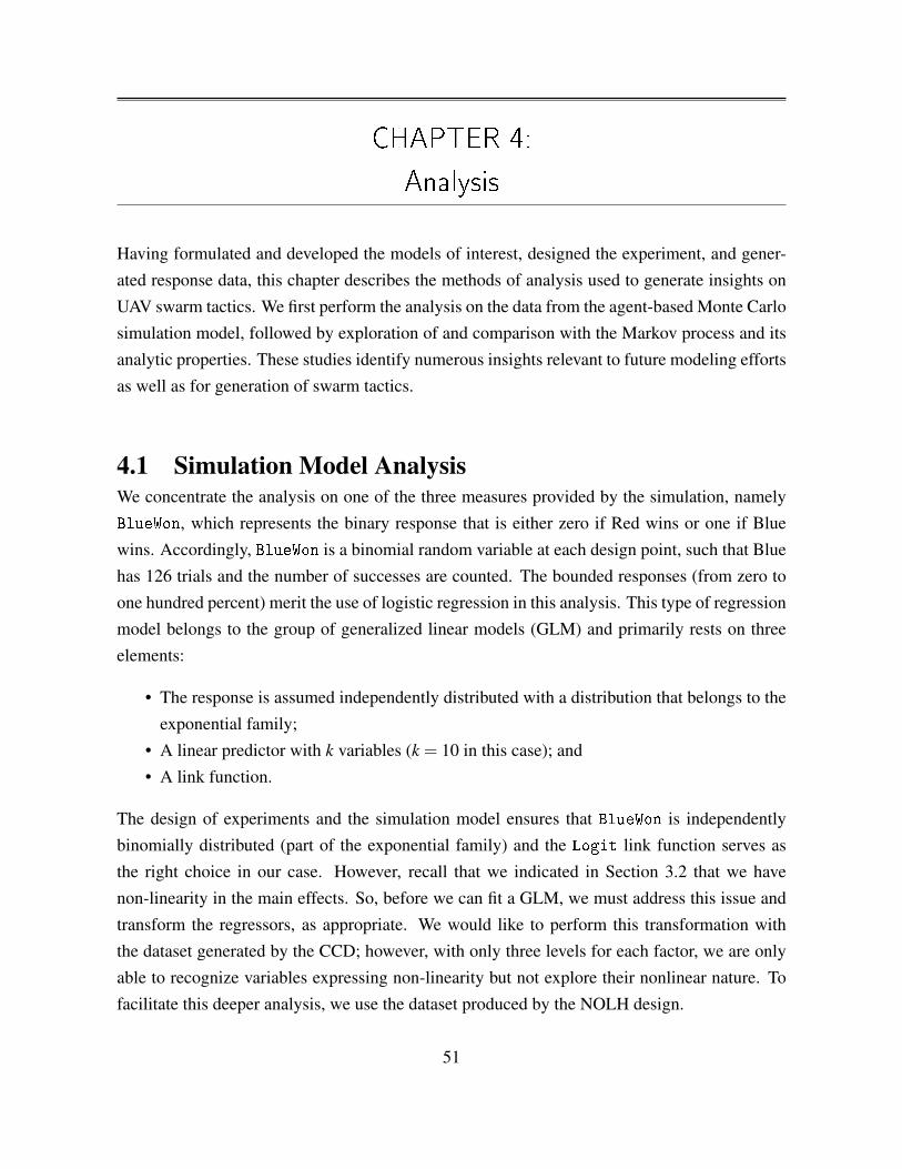
CHAPTER 4:
Analysis
Having formulated and developed the models of interest, designed the experiment, and gener-ated response data, this chapter describes the methods of analysis used to generate insights onUAV swarm tactics. We first perform the analysis on the data from the agent-based Monte Carlosimulation model, followed by exploration of and comparison with the Markov process and itsanalytic properties. These studies identify numerous insights relevant to future modeling effortsas well as for generation of swarm tactics.
4.1 Simulation Model AnalysisWe concentrate the analysis on one of the three measures provided by the simulation, namelyBlueWon, which represents the binary response that is either zero if Red wins or one if Bluewins. Accordingly, BlueWon is a binomial random variable at each design point, such that Bluehas 126 trials and the number of successes are counted. The bounded responses (from zero toone hundred percent) merit the use of logistic regression in this analysis. This type of regressionmodel belongs to the group of generalized linear models (GLM) and primarily rests on threeelements:
• The response is assumed independently distributed with a distribution that belongs to theexponential family;
• A linear predictor with k variables (k = 10 in this case); and• A link function.
The design of experiments and the simulation model ensures that BlueWon is independentlybinomially distributed (part of the exponential family) and the Logit link function serves asthe right choice in our case. However, recall that we indicated in Section 3.2 that we havenon-linearity in the main effects. So, before we can fit a GLM, we must address this issue andtransform the regressors, as appropriate. We would like to perform this transformation withthe dataset generated by the CCD; however, with only three levels for each factor, we are onlyable to recognize variables expressing non-linearity but not explore their nonlinear nature. Tofacilitate this deeper analysis, we use the dataset produced by the NOLH design.
51

4.1.1 Assessing the Raw Response DataBefore we start with the analysis, we take a look at the data and especially at the the responses.We can use the data, particularly the responses, from the CCD, as this design is used to fitthe initial model. Let us first conduct the transformation of parameters relevant to the initialspatial positioning of the Blue swarm (namely, yAlpha, yBeta, zAlpha and zBeta) into sur-rogate parameters, DistanceCenter and DistanceUAV, representing more tactically relevantdescriptions. Both regressors are shown in one plot in Figure 4.1. Observe that we do notfill the space due to the nature of the fractional factorial design, as expected. However, wesee a diversity of initial positions represented. For example, low DistanceCenter and lowDistanceUAV give a configuration representing an amassing of forces centrally in the airspace,low DistanceCenter and high DistanceUAV provide a positioning where the main force issplit on both flanks, and high DistanceCenter and low DistanceUAV concentrates the UAVswarm initially on one flank.
Figure 4.1: Scatter plot showing DistanceCenter against DistanceUAV design points. The centralcomposite experimental design can be seen to not be space filling; however, the clusters roughly outlinedifferent tactical configurations, namely (a) concentrated forces in the center of the field, (b) positioningon one flank only and (c) strong flanks, that is, forces amassed on both flanks.
There will never be data points with high DistanceCenter and high DistanceUAV becausehigh DistanceCenter requires all UAVs to be together on one edge but this reduces the dis-tance between the UAVs. So, we will never observe a balanced design for these two factors.
As we refer to Figure 4.2, we see that all regressors have a centered median except DistanceCenter
52

and DistanceUAV. The CCD is not space filling like an NOLH design but it still spreads theregressors evenly over the whole range. Unfortunately, we do not find this to be the case forDistanceCenter, which is nearly but not quite centered, and DistanceUAV, which is far off.Nonetheless, these two derived variables provide more meaningful explanation of the tacticalpicture than the original α and β values as descriptors of the initial spatial configuration of theswarm.
Figure 4.2: This figure shows the balanced design as all medians are centered except DistanceCenterand DistanceUAV. The vertical axes show the range of the variables while the thick horizontal line ineach plot marks the median for this factor.
Next, we can compare the three response variables, the scale of which is shown in Figure 4.3.The mean of BlueWon is below 0.5, but this outcome is not unexpected, as we varied the ini-tial position and CohesionMax of the blue swarm against the uniformly distributed Red swarm.However, we observe both extremes where, in addition to cases of never winning, the Blueswarm achieves 100% probability of success for certain design point(s). Considering the sur-vival rate of both Blue and Red swarms (see Figure 4.3[b]), note that the numbers of survivingUAVs do not differ significantly between the swarms, where Blue has a higher mean but also ahigher variance.
Let us explore the responses where Blue has at least 90% likelihood of success, that is, ofdestroying the Red’s high value unit. Comparison of the distributions for this subset of data,
53

Figure 4.3: Overview of data of the three responses. The circles are the means and the horizontal linesthe median. Plot (a) shows a lower success rate for Blue as expected. Plot (b) expresses that bothsides have approximately the same number of surviving UAVs even if Blue has a higher mean. But thevariance is also higher.
see Figure 4.4, with the full response data shows significant differences for nearly all of thefactors, with median factor values at either their high or low levels. The only exceptions areDistanceCenter and DistanceUAV, whose distributions are similar to those of the completeresponse data set. This suggests that perhaps initial positioning, represented by these two fac-tors, does not affect the response, though further analysis is required to investigate if this is trulythe case (e.g., due to interactions). All other variables indicate that there is an underlying, yetto-be-determined, influence on the results. We specifically investigate the exact behaviors inSection 4.1.4. It is also interesting to see that a high Blue success rate implies higher losses tothe Blue UAV swarm, as seen by the low median value of SurvBlue.
4.1.2 Exploring Non-linearity in the ResponsesFor this portion of the analysis, we use an additive model where the usual regression coefficientsare replaced by smooth functions, which offers more flexibility in fitting compared to linearmodels. The point we want to take advantage of is the ability to plot the smooth functions, whichgives some idea of how the regression variables influence the response (see Faraway [32]). Ifwe examine these plots, we should be able to find suitable transformations for the main effects.
54
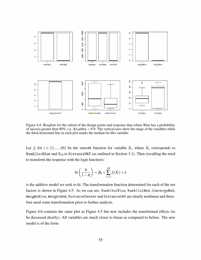
Figure 4.4: Boxplots for the subset of the design points and response data where Blue has a probabilityof success greater than 90%, i.e., BlueWon> 0.9. The vertical axes show the range of the variables whilethe thick horizontal line in each plot marks the median for this variable.
Let fi for i ∈ 1, ...,10 be the smooth function for variable Xi, where X1 corresponds toNumAllocBlue and X10 to DistanceUAV (as outlined in Section 3.1). Then (recalling the needto transform the response with the logit function):
ln(
π
1−π
)= β0 +
10
∑i=1
fi(Xi)+ ε
is the additive model we seek to fit. The transformation function determined for each of the tenfactors is shown in Figure 4.5. As we can see, NumAllocBlue, NumAllocRed, ConvergeRed,WeightBlue, WeightRed, DistanceCenter and DistanceUAV are clearly nonlinear and there-fore need some transformation prior to further analysis.
Figure 4.6 contains the same plot as Figure 4.5 but now includes the transformed effects (tobe discussed shortly). All variables are much closer to linear as compared to before. The newmodel is of the form:
55

Figure 4.5: Smooth function for all regressors with 95% confidence interval. The plots indicatethat NumAllocBlue, NumAllocRed, ConvergeRed, WeightBlue, WeightRed, DistanceCenter andDistanceUAV are nonlinear.
ln(
π
1−π
)= β0 +
10
∑i=1,i 6=9
fi(Xi) (4.1)
+β1t
√X1 + f2t (X
22 )+ f5t (X
25 )+ f6t (X
26 )+ f7t (X
27 ) (4.2)
+β9lX9l +β9tcX9c +β9trX9r + ε (4.3)
56

We can identify the appropriate transformations, with transformed functions and coefficientsdenoted by subscript “t,” and begin by transforming NumAllocBlue with a square root termwhich corrects the sine wave-form that we see in Figure 4.5. The transformed term does notneed a smoother in this case. For this first factor, the term is just modeled as in a regular linearregression, which we denote with the use of the regression parameter, β1t . Other parameters,namely NumAllocRed, ConvergeRed, WeightBlue and WeightRed, are fairly well transformedwith quadratic expressions (Line 4.2).
However, we could not find a suitable transformation for X9, or DistanceCenter. Anotherchoice in such a case is to perform piecewise linear regression. The variable is divided into twoor more intervals, and each part is treated as a linear regressor. The plot for DistanceCenter inFigure 4.5 indicates that there are three sections where each section could be modeled linearly,and the fitted lines would still be inside the confidence interval. Therefore, we have the left-handside in the interval [0,1500], the center in [1500,300], and the right-hand side in [3000,5500].This modeling technique is explained in Faraway [32]. Finally, we get the following functionaldescription, which replaces X9 with three components:
X9l =
1500−X9 ;X9 < 15000 ;X9 ≥ 1500
X9c =
3000−X9−1500 ;1500 < X9 < 30000 ;X9 ≤ 1500 or X9 ≥ 3000
X9r =
X9−3000 ;X9 > 30000 ;X9 ≤ 3000
With this piecewise linear representation, there is no need to further transform DistanceUAV,and we use the associated regression coefficients for the piecewise linear fits.
Having identified and addressed non-linearity issues in the main effects, in the next section wetake Equation 4.1 as the basis for the regression and add interaction terms in order to analyzethe simulation output.
4.1.3 Performing the RegressionWith the transformation steps complete, we are prepared to identify important variables andinteractions. The basic setup gives Equation 4.1, which enables the use of a linear predictor withthe chosen transformations and, thus, satisfies the elements of a GLM. We can now use logistic
57

Figure 4.6: Smooth function for all main effects and transformed terms with 95% confidence interval.
regression to fit the model; however, we still do not know if a first-, second- or third-ordermodel is sufficient in our case, that is, we do not know if two- or three-way interactions play asignificant role. Recall that the CCD exposes interactions up to the third order only compoundedby higher order terms. But do we really need these higher orders to capture insights from themodel? To answer this question, we fit three models, namely a first-, second- and third-ordermodel, and compare their predictive power. To ensure fairness of the comparisons, we anticipatehaving to normalize the regressors to the same scale to compare the chosen coefficients and todraw our conclusions before selecting one of these three.
58

Lasso RegularizationPrior to defining the various models, we begin by briefly explaining the proposed modeling ap-proach. We know that logistic regression is the right choice for a binomial response. However,instead of applying conventional approaches, we explore an alternative technique of lasso reg-ularization, which also provides a logistic model, but has at least three advantages in our case.First, lasso prevents over-fitting by restricting the complexity of the model, so we expect fewerterms. As we are interested in the most significant influences, identifying the simplest fit isadvantageous. Second, the results of both approaches are comparable and the small differencecan nominally be ignored with our purpose in mind. Third, the cross validation or variable se-lection part is computationally cheaper for lasso. In fact, we observe that it is nearly intractableto fit a third-order model in the normal way, while using the lasso approach takes only half anhour on an moderate computer. Lasso regression is further explained by Hastie, Tibshirani andFriedman [33].
The score function for a normal linear regression is the sum of squared errors
SSE = ∑i(yi− yi)
2
which is to be minimized. Instead, for lasso regularization, an additional penalty is included tocontrol the complexity and to prevent over-fitting, as seen in Equation 4.4.
SSE +λ
k
∑j=1|β j| (4.4)
The β s are the regression coefficients and λ is the tuning or complexity parameter, and mustbe chosen for a specific model. A common way to determine the tuning parameter is via crossvalidation. Equation 4.4 represents the new score function, which is to be minimized, whichdrives coefficients to zero and leaves fewer terms remaining in the model.The following sectiondescribes the application of the lasso regularization approach to our specific dataset.
Model ComparisonFor completeness, we conduct a comparison of the fitted models using both normal logistic re-gression and the lasso regularization approach, showing their similarity in results while the latterhas computational advantages. Before describing the application of the lasso process in detail,we provide a summary table comparing the fitted models. Table 4.1 shows the predicted mean
59

error and its standard deviation for varying order models for both the normal logistic regressionand lasso approaches. Note that in the case of the normal logistic regression, generation of athird-order model was untenable within reasonable computation.
order model measures normal LR Lasso
firstmean 0.196 0.196SD 0.00245 0.00273
secondmean 0.136 0.138SD 0.00211 0.00229
thirdmean 0.13SD 0.00223
Table 4.1: Comparison of different order models and regression techniques where mean it the error rate.The third-order model for normal logistic regression is intractable. But we assume that it would showalmost the same figures as Lasso regression according to the results for the first and second-order model.Overall, the third-order model does not improve very much compared to the second-order model.
First of all, we can see that both approaches provide nearly equivalent results for the first- andsecond-order models. We would assume that this is also the case for the third-order model.More important to note, however, is that the prediction error for the third-order model decreasesonly marginally compared to the second-order errors. We determine that the third-order modelprovides little additional benefit but requires the addition of many more terms. This increase inthe model’s complexity is undesirable; thus, we conclude that a second-order model is suitablefor the analysis of our data. Another point is that three-way interactions are hard to understand,to visualize, and to interpret, and we no longer have to address this issue.
As a note, the prediction power of the second-order model will be seen to be about 86%, whichis very good for the simulation model. In fact, we expected a smaller value because warfareis always uncertain. Nevertheless, this result leaves sufficient ambiguity to satisfy our intuitionand to convince us that we are on the right track. Table 4.1 summarizes the mean error rate forthe different models. The error rate for the second-order Lasso model is 14%, which can bedivided into type I errors, where the model incorrectly predicts a Blue success when it really isnot, and type II errors, where the model predicts a Blue failure when it is a success. The type Ierror is about 7.2% and the type II error is about 6.6%. In order to identify whether the resultsindicate a bias for either error type, we compare both with a two-sided t-test, where the nullhypothesis is that both are equal and the alternative is that they are different. The p-value forthis test is 0.0501 with a 95% confidence level, which is (barely) larger than 0.05, and as such,we do not reject the null hypothesis. Therefore, we do not see bias in one direction or the other,which provides further confidence in the analysis of the simulation model presented below.
60

The ModelIn this part we explain the modeling process in detail and describe how we arrive at the finallist of terms that are important in representing swarm vs. swarm combat. We start with thesimulation output for the CCD, which requires some pre-processing. Then we divide the data setinto a training set, which we use for cross validation, and a test set, which is used to determinethe prediction error. Afterwards, we can cross validate to choose the best λ for our model. Thisvalue also determines important main effects and interactions. Finally, we can compare thepredicted values with the test set. The statistics tool, R, is our choice to do all these computation.The packages gam and glmnet are used in addition to the standard R packages.
Let us start with the data set obtained from the simulation (see Table 3.4). For the immediateanalysis, we want to only explore BlueWon (Y3). Recall that we replace yAlpha, yBeta, zAlphaand zBeta by DistanceCenter and DistanceUAV. The final data set, in which we have thedesired one response and ten regressors is given in Table 4.2.
Y3 X1 X2 X3 X4 X5 X6 X7 X8 X13 X141 1 1 500 500 500 0 0 1 799 51641 1 1 500 500 500 0 0 1 360 52390 1 1 500 500 500 0 0 1 415 53060 1 1 500 500 500 0 0 1 317 52960 1 1 500 500 500 0 0 1 1030 5212...
......
......
......
......
......
Table 4.2: Modified data set for analysis purposes where Y3 is the column for BlueWon and X13 and X14are DistanceCenter and DistanceUAV, respectively.
We get this data format by importing the CSV-files mentioned at the end of Section 3.4 into Rand selecting the appropriate columns in the right order. Additionally, we transform BlueWon
into a factor as this is needed for the follow-on analysis.result = read . csv ( " . . . / r e s u l t D o E _CCD. csv " , header = TRUE )resultDoE = result [ , c ( 1 5 , 1 , 2 , 3 , 4 , 5 , 6 , 7 , 8 , 1 6 , 1 7 ) ]resultDoE$BlueWon = as . f a c t o r ( resultDoE$BlueWon )i s . f a c t o r ( resultDoE$BlueWon )
It is common practice to divide the available data into two sets, with one training set to fit themodel and one test set to determine how well the model predicts the unknown data. A rule-of-thumb suggests 10 to 25% of the whole data set should be used as the test set. We have 132,300observations in total. We conclude that 10% of these data points are suitable in our case, and sowe select randomly 13230 observations for the test set, denoted data.test, and have 119070
61

observations left in the training set, denoted data.train. The illustrative R code provides thispartitioning.
ran = sample (132300 , 13230)data . test = resultDoE1 [ ran , ]data . train = resultDoE1[−ran , ]
In the next step, we fit a saturated second-order model with normal logistic regression in orderto generate all the interaction terms. The function glm() does this, as illustrated below:
resultDoE . glm . lasso = glm (BlueWon~
( .−DistanceCenter+ lhs ( DistanceCenter , 1500) + center ( DistanceCenter , 1500 , 3000)+ rhs ( DistanceCenter , 3000)
) ^2+ I ( s q r t ( numAllocBlue ) ) + I ( numAllocRed ^2 ) + I ( convergeRed ^2 )+ I ( weightBlue ^2 ) + I ( weightRed ^2 )− lhs ( DistanceCenter , 1500) : center ( DistanceCenter , 1500 , 3000)− lhs ( DistanceCenter , 1500) : rhs ( DistanceCenter , 3000)− center ( DistanceCenter , 1500 , 3000) : rhs ( DistanceCenter , 3000)
f a mi ly =binomial ,data . train ,x = TRUE
)
Recall we divided the interval for DistanceCenter into three parts to solve the non-linearityissue of this regressor. This fact explains why we take out DistanceCenter and replace it withthe three parts lhs, center and rhs. We also add the quadratic terms. Finally, we remove theunnecessary interactions between the three parts of DistanceCenter.
The option x = TRUE ensures that the returned glm objects include a matrix with all terms andtheir values at each observation. This is a 119070 × 80 matrix in this case. We have 80 termsin the saturated model and want to choose the important ones.
x=data . matrix ( resultDoE . glm . lasso$x [ , −1] )
Next, we want to compare the fitted β js, but observe that the regressors are on different scales.For example, NumAllocBlue is defined in the interval [1,9] while ConvergeRed is in theinterval [500,1000]. Without addressing this issue, the resulting coefficients, β js, would bedifferent even if both have the same influence. We must first normalize the regressors to beon an equal scale, which can be performed using one of various methods. We choose one that
62

Montgomery and Runger [34] suggest, namely
zi =Xi− Xi
sXi
where Xi is the mean of variable Xi and sXi the standard deviation. If we do this normalizationwith all regressors (as follows), then all transformed factor value intervals have a mean of zeroand a variance of one.f o r ( i in 1 : ( dim ( x ) [ 2 ] ) )
xMean = mean ( x [ , i ] )xSD = sd ( x [ , i ] )z [ , i ] = ( x [ , i ] − xMean ) / xSD
We need the response in a separate vector for the glmnet() function which runs the lassoregularization,
y=data . train$BlueWon
after which we can run glmnet() and plot the results.resultDoE . lasso = glmnet (z , y , f a mi ly = " b i n o m i a l " )p l o t ( resultDoE . lasso , xvar=" lambda " , label=T )
How the choice of λ influences the magnitude of the different β js and the number of terms leftin the model is shown in Figure 4.7. The goal is to determine a λ that minimizes the scorefunction, that is, Equation 4.4. Function cv.glmnet() does this for us using ten-fold cross-validation, illustrated and described below (see [33]).
resultDoE . cv . lasso = cv . glmnet (z , y , f a mi ly = " b i n o m i a l " , maxit = 500000)p l o t ( resultDoE1 . cv . lasso )
The use of ten-fold cross-validation means that the data set (here denoted z) is divided randomlyinto ten partitions, and one of these partitions is always the validation set while the others areused to fit the model. In other words, the function fits ten models for every λ where everypartition is used as a validation set once. Then, the mean deviation and its variance is computedover the ten replications per λ . The results are shown in Figure 4.8. The deviation is smallestfor 78 terms present in the model. However, since all the deviations are only estimates and wewant the minimally complex model, such that cv.glmnet() uses the ”one-standard-error“ rulewhere a λ is chosen which is one standard error to the right of the minimum. Faraway [32] alsodescribes this method.
lambda . lasso = resultDoE . cv . lasso$lambda . 1 se
63

Figure 4.7: Lasso Regularization: Horizontal axis shows the log of the tuning parameter, λ (bottomaxis) which is equivalent to the number of terms left in the model (top axis). Vertical axis determinesthe size of the coefficients.
The choice of λ = 0.00022 is shown in Figure 4.8 with a dotted line slightly to the right from theminimum in the plot. Figure 4.7 contains a corresponding dotted line which marks the chosenλ -value. Finally, we are left with 74 main effects and interactions in the model.
The next step is to determine the prediction power of the model. We use the earlier separatedtest set for this purpose. Again, we must fit a saturated model with the glm() function first toget the x.test matrix and to standardize the variables. We only have to ensure that we usethe means and standard deviations we obtained earlier from the training set. Then we predictthe ys for the test set. All of these values are in the interval [0,1]. Recall that the responsevariable, BlueWon, is binary, that is, either 0 or 1. The inline R function result below is usedto conclude 0 if y is below 0.5 and 1 if y is above 0.5.
y . hat . lasso = p r e d i c t (resultDoE . lasso ,type = " r e s p o n s e " ,newx=z . test ,s=lambda . lasso
64
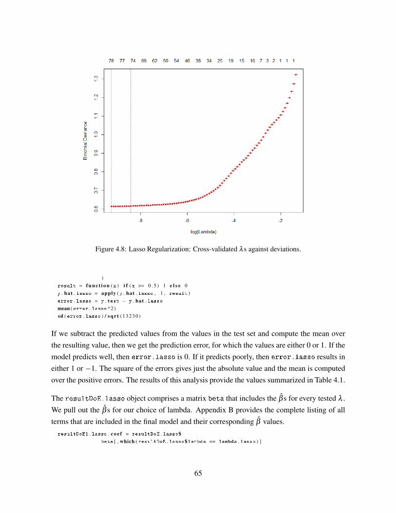
Figure 4.8: Lasso Regularization: Cross-validated λ s against deviations.
)result = f u n c t i o n ( x ) i f ( x >= 0 . 5 ) 1 e l s e 0y . hat . lasso = apply ( y . hat . lasso , 1 , result )error . lasso = y . test − y . hat . lassomean ( error . lasso ^2 )sd ( error . lasso ) / s q r t ( 1 3 2 3 0 )
If we subtract the predicted values from the values in the test set and compute the mean overthe resulting value, then we get the prediction error, for which the values are either 0 or 1. If themodel predicts well, then error.lasso is 0. If it predicts poorly, then error.lasso results ineither 1 or −1. The square of the errors gives just the absolute value and the mean is computedover the positive errors. The results of this analysis provide the values summarized in Table 4.1.
The resultDoE.lasso object comprises a matrix beta that includes the β s for every tested λ .We pull out the β s for our choice of lambda. Appendix B provides the complete listing of allterms that are included in the final model and their corresponding β values.
resultDoE1 . lasso . c o e f = resultDoE . lasso$beta [ , which ( resultDoE . lasso$lambda == lambda . lasso ) ]
65

betas = as . matrix ( resultDoE . lasso . c o e f [ resultDoE . lasso . c o e f ! = 0 ] )
The final model comprises 75 terms, indicating that only five terms of the saturated second-order model are not important to explain the response. This number of significant factors isquite a lot, as we expected to see fewer terms in the model, that is, only a handful of significantfactors. We also see that, even having standardized the variables, the range of coefficient valuesis still large (as seen in Appendix B). We concentrate further analysis on those terms that aredeemed more important or relevant to the scenario, rather than trying to explain the sensitivityfor all factors. As a method for drawing this line, we decide to take the mean of the β s andexplore those terms with a β larger than the mean. The resulting set of terms we discuss in thenext section, are shown in Table 4.3.
Term β
weightRed -2.40700031convergeRed -2.34268830I(convergeRed^2) 2.02622621I(weightBlue^2) 1.75709594weightRed:rhs(DistanceCenter, 3000) -1.63271293numAllocBlue:weightBlue -1.30740299numAllocRed:weightRed 1.08292601weightRed:stayingPwHVT 1.04541938weightBlue:stayingPwHVT -0.97929942weightBlue 0.82523436numAllocRed:stayingPwHVT -0.79081038weightBlue:weightRed -0.70730609convergeBlue:weightBlue 0.69240074numAllocBlue 0.68324259convergeRed:weightRed -0.66977778DistanceUAV -0.65948801weightRed:DistanceUAV -0.61042046cohesionMax:weightBlue -0.57027147numAllocBlue:stayingPwHVT 0.55291950weightBlue:rhs(DistanceCenter, 3000) -0.47040495cohesionMax:DistanceUAV 0.40974145numAllocRed:weightBlue -0.40864333cohesionMax:weightRed 0.39484181
Table 4.3: Most influential main effects and interactions in the final model and their coefficient values.
66

4.1.4 ResultsHaving performed the above rigorous statistical analysis to provide a regression model thatdescribes the response, we can begin to draw conclusions based on the fitted coefficients. Itseems the idea of variable selection does not work in this case because even if not all maineffects appear as important, they are at least represented in the interaction terms. Therefore, wecannot conclude to reject any of the used variables in the simulation. Next, we want to discussthe terms that have the highest significance according to the magnitude of their fitted coefficient.
WeightRed and ConvergeRed have the largest (absolute) β -values, with values below −2, sig-nifying that these two are the most important factors in this model. From Blue swarm’s per-spective, this fact is disheartening as both variables are controlled by the Red swarm’s tacticalchoice. For example, we see that β7 =−2.41, which means that a higher weight factor chosenby the Red swarm (i.e., Red swarm agents are more offensively driven than not) decreases theBlue swarm’s effectiveness and likelihood of destroying the Red’s high value unit. In fact, ifwe delve further by examining the interaction plot of the weight factors for the Blue and Redswarms, respectively, shown in Figure 4.9, then we observe that Red must simply maintain ahigh weight factor, and Blue’s choice no longer has any influence on the result. Recalling thatBlueWon is Blue swarm’s success rate, we see that Red simply must choose a weight factor offive or above to decrease Blue’s success dramatically.
Figure 4.9: Interaction of the weight factor for the Blue and Red swarms. This plot says that as long Redmaintains a high weight factor it is able to decrease Blue’s probability significantly. Blue’s choice doesnot matter in this case.
Another perspective is to look at the number of surviving UAV on both sides. Figure 4.10shows these values, namely SurvBlue and SurvRed, as a function of the Red swarm’s choice
67

of weight factor. The plot shows that the Blue swarm dominates with respect to its survivingforce ratio as Red uses a higher weight factor. Though it might lose its high value unit first tothe aggressively offensive Red swarm, the Blue swarm retains much of its UAV fleet and wouldnominally be able to counter-attack and destroy the Red’s high value unit as well.
Figure 4.10: Surviving Blue and Red UAVs at the end of the engagement for different red weight factors.
This disparity between the success measure (i.e., BlueWon) and the surviving UAVs measures(i.e., SurvBlue, SurvRed) highlights a current limitation of the agent-based simulation modelin its implementation. Rather than terminating the simulation after the first HVT is destroyed,the simulated scenario should continue to execute until both HVTs are destroyed (or until oneside is completely dominated, i.e., all of its UAVs and its HVT are destroyed). Such a modifiedtermination criterion would lead to draws as well, and as such, different priorities or weightingsfor successes and draws would change the analysis and the findings presented in this work. Theextension to this enlarged scope of the scenario is left for follow-on studies.
Continuing with the analysis, recall that we transformed ConvergeRed with a quadratic effectin order to solve non-linearity in the main effect. Both linear and transformed terms associatedwith ConvergeRed appear as significant factors in the regression, and merit further explorationof the impact. ConvergeRed and response variable BlueWon are shown in Figure 4.11. Recallthat ConvergeRed defines the distance to the Blue HVT at which a Red UAV starts to fly directlytowards it. In other words, until the range is less than the ConvergeRed threshold distance, theUAV flies roughly towards the Blue half but not directly towards the HVT. Therefore, a highervalue means that the swarm agents begin to converge and target the enemy HVT earlier (i.e., atgreater range). The plot indicates that maintaining a more dispersed formation is more beneficial
68

for Red than converging too early in the transit; however, this effect turns around at some point,where at approximately midfield, (approximately at a distance of 4750 m from the Blue HVT),there is an inflection point where concentrating forces initially provides a tactical advantage.The design implemented in this study does not provide sufficient resolution to determine theexact point, but can be conducted in near-term future research.
Figure 4.11: Influence of ConvergeRed and the quadratic transformation on the response. There is asaddle point somewhere around 5000 meters. The swarm should should wait with the final attack on theHVT, but also not too long.
Despite already knowing that Blue’s choice of WeightBlue has little influence on the outcomeif Red chooses a high weight factor, we still wish to explore this effect as it appears importantaccording to the magnitude of the regression coefficient, with an emphasis on the quadraticnature of the dependency. Indeed, if we look at Figure 4.12, we see a bigger increase in thesuccess rate for higher weight factors. Accordingly, Blue should maintain a high weight factorin general as this tactical approach is more beneficial, noting that the present simulation studyemphasizes first kill of the opponent’s HVT (rather than including draw conditions).
Another interesting analysis point appears in exploring the impact of the initial positioning ofthe swarm agents. The coefficient for the interaction between WeightRed and DistanceCentersignifies its importance. The different slopes for different weight factors are shown in Fig-ure 4.13. More important, however, is the fact that we see a decreasing success rate with in-creasing distance from the center; that is, increasing DistanceCenter. DistanceUAV is theother factor that describes the initial positioning. The coefficient is negative and suggests thata more compact formation is more beneficial. Therefore, the best Blue can do is a centeredand concentrated initial configuration. This tactical choice makes sense as WeightRed is high
69
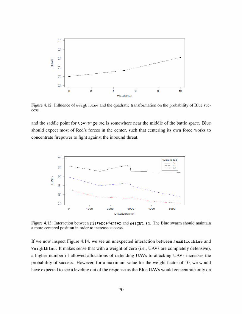
Figure 4.12: Influence of WeightBlue and the quadratic transformation on the probability of Blue suc-cess.
and the saddle point for ConvergeRed is somewhere near the middle of the battle space. Blueshould expect most of Red’s forces in the center, such that centering its own force works toconcentrate firepower to fight against the inbound threat.
Figure 4.13: Interaction between DistanceCenter and WeightRed. The Blue swarm should maintaina more centered position in order to increase success.
If we now inspect Figure 4.14, we see an unexpected interaction between NumAllocBlue andWeightBlue. It makes sense that with a weight of zero (i.e., UAVs are completely defensive),a higher number of allowed allocations of defending UAVs to attacking UAVs increases theprobability of success. However, for a maximum value for the weight factor of 10, we wouldhave expected to see a leveling out of the response as the Blue UAVs would concentrate only on
70

the Red HVT and not aim to defend against Red UAVs. This behavior does not seem to be true.Having already stated that Blue should maintain a high weight factor, NumAllocBlue shouldnominally be kept low. Hence, an intermediate value for the weight factor between the low andthe high levels does not benefit the Blue swarm’s effectiveness. Rather, WeightBlue shouldeither be at high or low levels, with NumAllocBlue chosen accordingly. This insight impliesthat a homogeneous UAV swarm fleet should be designed for pure offense or pure defense, withlittle benefit of a mixed strategy. However, future research could investigate heterogeneous
swarms, either by platform or by task assignment, where some agents are designated for theoffensive strike mission and others are specifically reserved for defensive countermeasures toattacking UAVs.
Figure 4.14: Interaction between NumAllocBlue and WeightBlue. A high Blue weight factor demandsa low number of allocations and vice versa.
Further inspection of the relationship between NumAllocRed and WeightRed yields a similarrelationship, shown in Figure 4.15, as seen previously; that is, Red should also choose a lownumber of allocations in order to support a high weight factor.
The next two plots in Figure 4.16 also illuminate an interesting behavior. A low staying powerof the HVTs (assumed the same for both sides) favors a high Blue weight factor, and conversely,a high staying power implies using a low Blue weight factor. One reasonable explanation couldbe that the losses experienced with a high weight factor are too great to retain sufficient forcesto achieve the main objective. We see an analogous behavior for Red (noting that red’s objectiveis to minimize BlueWon). Therefore, according to the presented analysis, the assumed stayingpower of the respective high value units should appropriately inform the choice of the weightfactor for at least the blue swarm.
71

Figure 4.15: Interaction between NumAllocRed and WeightRed. Again, the number of allocationsshould be high if the weight factor is low and contrariwise.
Figure 4.16: Interaction between StayingPwHVT and WeightBlue (a)/ WeightRed (b). StayingPwHVTcannot be controlled by the swarm and is therefore the basis for the choice of the weight factor. Blueshould have a high weight factor for a low staying power and vice versa. Red does best with a highweight factor every time.
A final conclusion that merits mentioning is that CohesionMax turned out to not carry as muchimportance as we might have expected, as more coordination in swarm motion may have as-sisted in keeping forces concentrated. In fact, the coefficient is negative and suggests that strongcohesion of the swarm does not provide a benefit. This result also speaks to a broader questionof the value of coordination among distributed agents, and perhaps the benefit or penalty therein.Recall, however, that cohesion is only one of three parts that define the swarming behaviors im-plemented in the simulation model, among shared broadcast communication of detected targets
72

and local negotiation of target allocations. We have not investigated these capabilities with thecurrent simulation study because both swarms are treated as possessing identical coordinationcapabilities. A richer future analysis that explores the advantages or disadvantages of varyingcoordination levels as well as disparities in their implementation between Blue and Red swarmswould likely be an interesting and insightful avenue of research.
4.1.5 Sensitivity AnalysisThe presented results in the previous section provide general insights on how values should bechosen for the defined parameters in our scenario to maximize the success of either side. Inthis section, we consider specific recommendations and construct a new design point reflectingthose insights, as described in Table 4.4.
Variable Name ValueNumAllocBlue 9NumAllocRed 9CohesionMax 500ConvergeBlue 10000ConvergeRed 5000WeightBlue 10WeightRed 10StayingPwHVT 6YAlpha 1001YBeta 1001ZAlpha 1001ZBeta 1001
Table 4.4: Parameter setting for additional analysis.
Given that the staying power of an HVT is a function of the asset itself and is consideredoutside the influence of the swarm parameters, we choose a nominal value of six. All otherparameters are dictated by the swarm, and guided by the insights obtained earlier. Recall thatthe weight factor is the most important parameter for both Red and Blue swarms. We thereforechoose a value for this variable first. As it interacts with staying power, we set WeightBlueand WeightRed to ten for both swarms. The choice for the number of allocations also dependson the weight factor, and based on Figures 4.14 and 4.15, this parameter should be set to onefor both Red and Blue. We also concluded that cohesion should be as low as possible, forwhich a defined range of 500 meters is an appropriate value. We set ConvergeRed to a value of5000 because we have the quadratic influence that exhibited an inflection point approximatelynear this value. On the other hand, ConvergeBlue does not exhibit a nonlinear effect, and
73

its regression coefficient (refer to Appendix B) is positive. Hence, the parameter should be aslarge as possible, with 10000 meters as the maximal range. Finally, we configure the values forspecifying the initial positioning. The analysis in Section 4.1.4 suggests a centered and closedsetup, which we obtain if both distributions are symmetric and have a low variance. This is thecase if Alpha and Beta have approximately the same value and are as large as possible, namelya value of 1001. Note that the Red forces are still uniformly distributed in the pre-positioningbin.
We run this design point with 1000 replications and conduct a two-sided t-test on the BlueWonmeasure, where the null hypothesis is that Red and Blue have an equal chance of success andthe alternative is that the probabilities to succeed are different.
H0 : pblue = pred
Ha : pblue 6= pred
Recall that the MOE is defined to be one for a Blue success in a given single run and zero for aRed success. Therefore
pblue =∑BlueWon
1000pred = 1− pblue
are the mean probabilities for a Red and Blue success.
The t-test shows that pblue = 0.532. The p-value is 0.043 and therefore below 0.05. Hence, wereject H0 and Ha is true, performed and output in R as follows.> t . test ( resultDoE . data $BlueWon , alternative = " two . s i d e d " , mu = 0 . 5 )
One Sample t−testdata : resultDoE . data $BlueWont = 2 . 0 2 7 , df = 999 , p−value = 0 .04293alternative hypothesis : true mean i s not equal to 0 . 595 percent confidence interval :0 .5010208 0 .5629792sample estimates :mean of x
0 .532
For the selected design of the swarm systems, Blue has the advantage in this particular case.The main disparity arises due to the initial positioning of both swarms, as the Blue swarmspecifically selected its initial spatial configuration, which is superior to the Red’s uniformlydistributed positioning.
74

4.2 Markov Process AnalysisWith the in-depth simulation analysis performed, this section investigates insights generated bythe analytic formulation of the swarm-versus-swarm engagement using a Markov process modelintroduced in Section 2.3. By designing and assigning values to the defined probabilities andrunning the formulated computations, we can analyze the steady state properties of the model,followed by further study of its sensitivity to these transition probabilities.
4.2.1 End State AnalysisWe begin this analysis by summarizing the appropriate transition probabilities and their as-signed values in Table 4.5 (with discussion of the design choices following), which recalls thedefinitions presented in Table 2.3.1. Recall by construction that definition and design of theseprobabilities is sufficient for both the one-on-one and swarm-versus-swarm engagements, sincethe latter leverages the estimates constructed in the former.
Probability Valuep0,HR = p0,HB = pB,HR = pR,HB = pB,HB = pRHR 0.01p0,B = p0,R 0.49pB = pR 0.60pB,R = pR,B 0.10pB,0 = pR,0 0.28
Table 4.5: Transition probabilities for the one-on-one combat (first level) Markov process.
The values chosen for this first level Markov analysis are presented as nominal, representativevalues. We define the baseline case where both sides are assumed to be balanced, in bothforce strength (UAV swarm size) and swarm capabilities (identical forces). The transitions tothe states, HVTR and HVTB, should be rare events because the UAVs are required to transit tothe HVT and will most likely encounter opposing UAVs which force them into dogfights. Wespecify this notional value as 0.01. We do not differentiate between the different source statesbecause we do not have any evidence that there are differences.
The model starts always in state 0, the unengaged state. The probability for either side to reacha favoring state should be 0.5 in order to reflect equal forces. The next possible states, startingin state 0, are HV T R, BvR, HV T B and RvB where 1 = p0,HR + p0,B + p0,HB + p0,R. Two of thestates are preferred by Blue and two by Red. Therefore
75

p0,HR + p0,B = 0.5p0,HB + p0,R = 0.5
and it follows
p0,B = 0.5− p0,HR = 0.49p0,R = 0.5− p0,HB = 0.49
as we already fixed p0,HR and p0,HB.
The probabilities, pB and pR, describing the successful defeat of an opposing UAV are similarlyassumed to be equal, since both have an equal chance to get into a firing position and shoot theopposing UAV down. We set this value to 0.6 to reflect that, given identical platform types, it ismore likely that the evader is taken out of action than it is to manage to evade or to reverse rolesand become the pursuer itself. We assume that it is harder for an evader to become a pursuer(again, due to the equivalent platforms) than to escape the pursuit, for which we set pB,0 andpR,0 to 0.28 and pB,R and pR,B to 0.1.
Now we can use Table 2.3.1 and Equation 2.1 to compute the steady state probabilities, pre-sented in Table 4.6. Each instance of combat always starts in state 0. Therefore we are onlyinterested in the first row of the table which comprises the end state transition probabilities fromstate 0 to all four end states.
B R HVTR HVTB0 0.47 0.47 0.03 0.03BvR 0.75 0.21 0.02 0.02RvB 0.21 0.75 0.02 0.02
Table 4.6: Steady state probability matrix for one-on-one combat (level1).
As expected due to the symmetry of construction of this baseline case, both Red and Blue UAVshave an equal chance to down the opposing UAV and the odds of individually destroying theenemy HVT are low.
We take these four steady-state probabilities and use them for the second level as formulated inSection 2.3.2. We again apply Equation 2.1 to the swarm-versus-swarm transition probabilitymatrix presented in Table 2.3.2, and compute the steady state probabilities for the multi-UAV
76

engagement. Rather than showing matrix B2 in its entirety, we present Figure 4.17 which illus-trates the steady state probabilities graphically. Recall that in this swarm-versus-swarm case,the model always starts in the state 50/50, allowing us to only consider the probabilities fromthis initial state to one of the end states.
Figure 4.17: Steady state probabilities for multi-UAV engagement. A destroyed HVT is much morelikely than a completely defeated swarm.
We can see that a destroyed HVT is most likely, while the probability of having one side com-pletely eliminate the opposing swarm is almost zero. This fact can be easily explained, as theMarkov process has the same issues as the simulation model discussed previously, in which theprocess is assumed to terminate (by design of the absorbing states) as soon as an HVT is takenout of action. The number of surviving UAVs on both sides does not play a role in either the pre-viously or presently described models. Though such extensions can be implemented in futurestudies to generate a more realistic operational scenario (in which the fight does not necessarilyend as modeled), the fact that both the simulation and the theoretical models show analogousbehaviors helps convince us that the studies are consistent.
4.2.2 Sensitivity AnalysisThe baseline model above assumes both sides are totally balanced, but fails to provide interest-ing insights that could be used as decision recommendations. We wish to explore variations ofthis model and their behavior in greater detail in this section. In order to do so, we change one
77

or two of the transition probabilities in level one (individual UAV engagements) and observe itsimpacts on the swarm versus swarm context.
Results of these variations, such as shown in Figure 4.17, provide a starting point. Note that they-axis is not linear, to show that there is at least a small chance that a swarm is totally defeatedand HVTR and HVTB are not the only end states with steady state probabilities greater than zero,albeit nearly so. For this reason of scale and for purposes of identifying general insights, weuse a scenario with 10 versus 10 UAVs in this section. As such, the probability values are lessextreme while still enabling easier exploration and understanding from the model while tellingthe same story as the envisioned 50 versus 50 UAV swarm model.
First, we want to explore the influence of the HVT end states. We already saw that both HVTend states have a high steady state probability. How does this change if we decrease or increasethe transition probabilities? An increase in probability in a given transition would force thattransition to the end states more likely, or alternatively a decrease in the probability to switch toother states, such as a decrease in the likelihood to get into a dogfight and perhaps correspond-ingly, reflect a more offensive attack preference. We discussed such a behavior previously aswe identified the weight factors in the simulation model as the driver of offensive versus defen-sive agent-based behaviors. These transition probabilities of engaging the HVT provides thisconnection between the two modeling formulations. For further study, we fix Red’s transitionprobabilities and change only Blue’s values, p0,HR, and tying other parameters accordingly, i.e.,p0,HR = pB,HR = pR,HR, as these parameters relate to the offensive attack preference of the Blueagainst the Red HVT. The probabilities vary from 0.0001 to 0.02, and we observe results wherep0,HR ≤ p0,HB = 0.01 and p0,HR ≥ p0,HB = 0.01. Figure 4.18 indicates these state transitionsare a dominant factor in the model, as it can be seen that Red has the advantage (i.e., the BlueHVT is most likely destroyed) for low values of p0,HR. However, as p0,HR increases, the likeli-hood of arriving at the end state where the Red HVT is destroyed increases quickly, noting thatall other steady state probabilities are decreasing as well.
Important to note is the similarity in Figure 4.18 as was observed in Figure 4.17, but on a dif-ferent scale. This straightforward ability to scale the probabilities according to the swarm sizesprovides flexibility in our analysis, allowing easier understanding of the sensitivities regardlessof whether studying the 10 versus 10 or the 50 versus 50 UAV scenarios.
As another area to explore, what if we do not assume identical UAVs for both sides, such thatone side has a tactical advantage over the other in one or more characteristics? The value of
78

Figure 4.18: Steady state probabilities for different values of p0,HR (or equivalently, pB,HR and pR,HR).The magnitude of this probabilities refer to the weight factor in the simulation model. The plot showsthat an offensive swarm is superior to a more defensive one.
this sensitivity analysis is to show how much tactical advantage is necessary to achieve a de-sired specified success rate, which then has impacts on system-level design and developmentof UAV platforms. In order to explore this space, we vary p0,B and p0,R, which reflect theprobabilities of the Blue or Red UAV, respectively, entering an engagement with the edge. Inother words, p0,B gives the probability that a Blue and a Red UAV enter into a dogfight whileboth are previously unengaged, and that Blue has the advantage. Recall that all outgoing edgesof a given state must sum to one, such that if we increase p0,B, for example, we necessarilymust decrease p0,R. For the presented example, consider p0,B to range from 0.09 to 0.89, withchanges to p0,R accordingly. Values p0,B > p0,R imply that the Blue UAVs have better capabili-ties (e.g., enhanced speed, sensors, swarm performance) or better tactical position (e.g., higherflight ceiling). These kinds of behavior also influence the states BvR and RvB. For example,assume p0,B + p0,HR = 0.6 and consequently p0,R + p0,HB = 0.4, and Blue pursues Red (i.e.,state BvR). Then we would expect that pB increases and pBR and pB0 both decrease due tothe better performance of Blue. That is, Red has less opportunities to decide the outcome of
79

the engagement. Conversely, these correlations also hold for RvB. The mentioned probabilitiesare changed proportionally to the change in p0,B + p0,HR. In our example, p0,B + p0,HR = 0.6and therefore there is a change of 10% compared to the baseline model in Section 4.2.1 wherep0,B + p0,HR = 0.5. Then pB = 1−0.9 · pBR−0.9 · pB,0− pB,HR− pB,HB. This decrease in pBR
and pB,0 and the increases in pB reflect Blue’s better performance.
Figure 4.19 shows that the likely benefit of substantial investment in better platforms or payloadsmay only be marginal, as the technologically inferior side still wins in 25% of all cases regard-less of investment level. Such technological enhancements are not only likely to be costly, theadvantage is often also only temporary as the technology proliferates. A cost-benefit analysiscan be performed as future work to more definitely address this trade space.
Figure 4.19: Blue success probability as function of p0,B and p0,R. Even if one side has a large perfor-mance advantage, the opponent swarm still keeps a relatively high success probability.
Now we want to combine the former two analyses. We vary p0,B between 0.09 and 0.89 asbefore, while p0,HR, pB,HR and pR,HR range from 0.0001 to 0.02. We observe the same generalbehavior in Figure 4.20 as in the analyses before. However, the results also indicate that adaptedtactics can offset inferior performance. p0,HR, pB,HR and pR,HR can be interpreted as the weightfactor we defined for the simulation model. They determine the offensive and defensive be-haviors of the swarm and is one part of swarm tactics. Even if Blue has a lower performancecompared to the Red swarm, it is able to keep almost a 0.5 success rate by increasing the weight
80

factor. On the other hand, performance comprises not only hardware capabilities but also ”softskills“ which include elements of swarm tactics. One important point is coordination amongthe swarm UAVs. For example, blind spots in the sphere around the swarm due to limitedsensors could be mitigated by friendly UAVs actively fly to provide visibility of these knownareas. Such additional coverage would increase the performance and offset a potential disad-vantage. Based on these conclusions, we can observe that cost-intensive and time-consuminghardware changes may not only provide marginal improvement to the system, but that emphasison coordination tactics for cooperating UAVs may provide even greater enhancements.
Figure 4.20: Blue success probability as function of p0,B and p0,HR. The horizontal plane indicates the0.5 success probability. A more offensive strategy can raise the success probability even though theperformance is poor compared to the adverse swarm.
The analysis in this chapter identified important factors for UAV swarm tactics. For example,the weight factor governing offensive versus defensive preferences for the swarm turned outto be most significant for the defined scenario. Furthermore, we saw that the simulation andMarkov process models lead to similar results which increases the confidence in the respectivemodels. The advantage of the agent-based simulation model is the ability to investigate specificagent-level parameters and their impact on the swarm engagement, whereas the advantage of theMarkov process formulation is that it enables sensitivity studies, including analysis of opposing
81

swarms of different capabilities (e.g., better platforms). Though both models can be enhancedto provide greater representation of a more realistic engagement, such as including draws, theinsights provided in this thesis provide a basis for future recommendations and development ofswarm systems and their tactics.
82

CHAPTER 5:
Conclusions and Future Work
5.1 ConclusionsThe main objective for this thesis was to identify important factors that influence UAV swarmtactics. Though one could argue that such tactics development is not different from that formanned air combat, the basic conditions and engagement scenarios are not equivalent. Thefuture warfare concept explored in this thesis addresses the employment of inexpensive andexpendable platforms compared to their expensive and necessarily recoverable manned fighteraircraft counterparts. The loss of such a UAV also does not risk the life of a pilot. Further, itis conceivable that it could also be tactically beneficial to sacrifice UAVs in order to destroyan adversary’s HVT. These tactics are surely different from combat where humans are directlyinvolved. Moreover, we assume autonomous swarms with little to no direct control of individualUAVs by a ground station. In the ideal case, perhaps all the knowledge and understanding ofan pilot should be implemented in the UAV. However, we know that this is technologicallyinfeasible, and as such, we focused more on identifying the basic elements in such swarm UAVengagements that make the difference.
There are at least three approaches to address and analyze this novel future concept of swarm-versus-swarm UAV warfare. First, we could strive to find a solution through theoretical abstrac-tions and apply historical cases to this new topic. Such an approach is likely a good point tostart; however, the complexity of the scenario and the analytic assumptions will likely overlookimportant influences. The second approach is to conduct real-world experiments. However,given that this is an advanced warfare concept, we do not yet have the technological capabilitiesto perform operational-level experimentation. The third approach lies in between these two,and this hybrid perspective provides the desired capability assessment tools. We chose two dif-ferent types of models, one being an agent-based simulation model and the other, a stochasticMarkov process as an analytical model. Both have different foundations and our hope is thatthey complement one another.
We identified and here highlight six elements connected to the tactics of an UAV swarm, whichmerited study in this design and assessment effort, including:
• The maximum number of allocations per detected enemy target,
83

• The distance from the adversary’s high value target at which the swarm starts to convergedirectly on this objective,
• The maximum distance relative to a UAV within which it recognizes swarm members forits cohesion behavior,
• A factor that describes a preference between offensive (i.e., attacking the HVT) and de-fensive (i.e., defending against attacking enemy UAVs) postures,
• The staying power of the high value target, and• The initial spatial configuration of the deployed UAV swarm.
In leveraging the statistical design of experiments to systematically explore the factor space, weused a central composite design to scan for the importance of twelve identified variables andtheir interactions. The carefully constructed experimental design was executed, generating thefollowing three response variables as measures of effectiveness:
• Blue success in destroying the Red HVT [yes/no]• Number of surviving Blue UAVs• Number of surviving Red UAVs
During the analysis portion of this thesis, we fitted a logistic regression model with Blue successas the response. The first key insight from this analysis is that all studied main effects are impor-tant. Either the main effects themselves are important or they are part of influential interactions.With an error rate of only about 14%, we developed a regression model that explains much ofthe variability in the simulation model, but allows for further study and sufficient uncertaintydue to the “fog of war.”
For the underlying scenario, it is important to destroy the opposing HVT before the adversaryswarm reaches one’s own HVT. The analysis showed that the outcome of the battle is signifi-cantly dependent on the Red swarm’s choices of parameters under the assumptions of the givenscenario. This effect could be due to the fact that, whereas the initial positions of the Blueswarm was varied substantially (to explore tactics involving one- or two-sided flank attacks orconcentration of forces in the center), the initial positions of the Red swarm were always uni-formly spatially distributed. The reduced variability of the Red swarm’s initial positioning isattributed with this asymmetry in significance. Based on the analysis, a uniformly distributedinitial configuration seems to be adaptable to most opposing situations, and overall appears tobe the best choice if one does not know anything about the enemy’s tactics.
84

The statistical analysis of the responses further highlighted specific insights with respect toseveral key swarm tactics attributes:
Weight factor: The analysis showed that the weight factors governing preferences for offensiveversus defensive behaviors are most important to mission success, with the Red swarm’s weightfactor playing a significant role. The Red’s value should be chosen high, such that the swarmprimarily concentrates on the main objective of attacking Blue’s HVT and nearly completelyignores the secondary objective of attacking incoming blue UAVs. The same relationship istrue for the Blue swarm, but not to the same magnitude. The advantage of such a behavior isintuitive, since the swarm can accomplish the mission despite suffering many losses, and sothere is not much benefit to the mission by attacking opposing UAVs in a defensive context.The analysis also showed that this weight depends (as an interaction) also on the staying powerof the HVTs. For a higher staying power, more UAVs are needed to destroy the HVT, such thatwe observed that a lower weight factor is more appropriate (e.g., for staying power equal toeleven).
Convergent distance: Another important factor is ConvergeRed. Based on the analysis, theideal choice for when attacking UAVs should begin converging on the HVT is approximatelyat the midpoint distance between the two HVTs. Recall that the experimental design we usedconsisted only of three levels per regressor, so the exact point cannot be determined. In contrast,ConvergeBlue as main effect does not appear to be very important, but we surmise that this factis also a result of the variability in the initial positioning of the Blue swarm. A design that variesthe Red positioning as well could explore this asymmetry.
Number of allocations: Interesting to note is the interaction between the weight factors andthe number of allocations (i.e., the number of defending UAVs assigned to a single enemyUAV). First of all, since the weight factors are more important than the number of allocations(see above), we should choose the number of allocations according to the choice of the weightfactor. The interactions show an inversely proportional positive relationship between the weightfactor and number of allocations (i.e., a low weight factor benefits most from a high number ofallocations and vice versa).
Initial positioning: Though hypothesized that initial deployment configurations would be im-portant for influencing mission performance, the analysis showed that it was less importantthan expected for the given scenario setup. We could not find an initial positioning of the Blueswarm other than a centered and concentrated configuration that yielded favorable results. In
85

fact, additional runs with an optimized parameter choice derived from the analysis for initialpositioning showed that such a concentrated and centrally-located configuration is superior tothe uniform distributed setup of the red swarm.
Cohesion: This variable is also less important, which was surprising, given its role in dictatingthe collective swarm flight behaviors. More interestingly, the analysis suggests a loose swarmconfiguration with less influence between swarming agents. However, this result is mitigatedby the choice of initial positioning, since all UAVs are nominally within each other’s cohesivesphere of influence when the initial configuration is relatively compact and concentrated.
Staying power: It is not important on its own, but as previously mentioned, this variable’sinteraction with the weight factors does play a role. However, given that the staying power ofthe HVT is not one that is explicitly chosen by the swarm, this fact dictates that the swarmshould choose its swarm tactics and parameters according to the given staying power of theswarm’s assigned HVT.
The analysis of the Markov process model showed that the theoretical formulation points inthe same directions as the simulation, which we had hoped to see, and assists in verifying thesimulation model. In addition, we were able to relate the choice of transition probabilities in theMarkov model to associated variables in the simulation model. As a result, we can leverage ananalytical model, which can be used for macroscopic and on-the-fly analyses of swarm tactics,and rely on the constructed simulation model that provides a more detailed investigation butrequires additional investment in conducting the analysis. The highlighted key insights intoswarm tactics as well as the formulation of these two complementary models to explore themin detail are the main contributions of this thesis.
5.2 Future WorkWe gained some insights about tactics in swarm versus swarm combat with the provided models.However, we have already identified several areas for improvement in the models themselves,in the analysis approaches, as well as in a deeper understanding of this topic of swarm tactics.
First of all, the generated regression models apply (and apply well) to the specific scenario stud-ied in this thesis. However, the scenario is not of sufficient fidelity whereby the results couldeasily be transferred to swarm tactics employed in the real world. The biggest weakness is thatthe scenario stops (i.e., the simulation terminates) as soon as one HVT is destroyed. The anal-ysis revealed that success of destroying the adversary’s HVT and the resulting force ratio are
86

not unrelated. Rather, though one swarm was able to accomplish the mission, it lost so manyUAVs that the remaining UAVs would not be able to protect the home base. Hence, both HVTswould be ultimately destroyed. This is a draw situation we do not presently allow in the currentscenario. A dominant victory accomplishes both the main and secondary objective where a de-feated UAV swarm is equivalent to a destroyed HVT. If we penalize a draw, perhaps analogousto draws in soccer, then the fitted model favors meeting the complete victory conditions. How-ever, this modification also changes the analysis as the primary measure of effectiveness is nolonger a binary response variable. Further, we must be cautious in applying the results foundherein in a real combat situation, since the present study assumed that the Red swarm utilizedthe same objective function as the Blue swarm, which need not necessarily be true.
If we go with the last statement, then it may be beneficial to know how the adversary swarmbehaves prior to the engagement. This highlights the advantage of performing good recon-naissance, for example, by dedicating a few of the UAVs to scouting missions. Another wayto address uncertainty in the opponent’s objective function could be to diversify and split theswarm into offense and defense components. Note, however, we saw the extreme cases wherethe friendly swarm is wholly defensive (weight factor is zero) and the adversary is offensive(weight factor is ten), in which case the offensive swarm has the advantage according to theinteraction plot from the analysis. One solution to counter this issue could be to increase thedistance between the home bases. Then the defense has more time to defeat the attackingswarm. Such line of reasoning, however, leads to additional questions, such as what is the idealstandoff distance? Though this could be another factor in future analysis, an increase in thisdistance between HVTs could have other operational considerations, especially when includingendurance limitations and ammunition consumption in extended models.
After addressing tactics-related avenues for future work, we also see promising extensions tothe simulation model formulation. We employ communication, sensors, and weapons systemsunder nearly perfect conditions in the model so far. However, in order to address uncertainty inwarfare and nature, we could introduce probabilistic distributions to model real-world effects,for example. But does this really improve the model and substantially change the results? Thislast question is an interesting one that cannot be answered without further investigation.
The analytical model has also some potential for improvements. First of all, we constructed thetransition probabilities, which were not based on any empirical observations neither from thereal world nor from other models. Given the future concepts nature of this study, we cannot
87

get real world data; however, the simulation system could provide estimates of these values.However, since the states of the individual UAV agent in the simulation do not directly matchthe states in the Markov process, this latter approach may pose some challenges. Furthermore,the current Markov process model only allows one-on-one combat, but not multi-on-one. Forsure, the number of possible states would grow exponentially, but short excursions with baselinetwo-on-one models, as found in the literature, could provide some insights. Another point forextension of the Markov model is the staying power of a HVT, which is constrained to be one,that is, the HVT can only sustain one hit. This limitation could be removed so as to furthercompare its results with those of the simulation model. Another way to model the scenariowith an analytical approach is the use of Lanchester equations, which notably were originallydeveloped to explore air-to-air combat. Though the resolution of this differential equation-basedapproach does not enable study of agent-to-agent interactions, it would be interesting to see howthe results compare to the Markov process and the simulation model.
Finally, the scenario we study assumes that there are two swarms of UAVs that have a sense ofcohesion, share knowledge of detected targets, and smoothly negotiate target allocations. Butan open question remains as to whether these capabilities really matter? What if one swarmdoes not have one or more of these capabilities? Such an interesting question could be straight-forwardly answered with the presented simulation model in near-term future work. Other mod-ifications of the scenario could include jamming, which reduces the communication capabilitiesamong the UAVs, or the challenge of unknown HVT positions, in which swarm search algo-rithms would be needed.
Overall, this thesis provides a first step into the complex world of swarm-versus-swarm tactics.Both simulation and theoretical models provide a basis for significant follow-on research. Inactuality, this thesis could not provide solid answers that are immediately transferable to theoperational world. However, the value and contributions of this thesis are that it has preparedthe stage with two tools, by sketching a way through the whole process and by identifyingadditional questions that are worthwhile to addressing.
88

APPENDIX A:
Simulation Environment Installation
Run the JARsWe provide three jar-files (Java Archive) with this thesis. All three can be downloaded fromhttp://faculty.nps.edu/thchung under Software.
• UAVSwarm_source.jar comprises the whole project with java and class files.• UAVSwarm.jar is executable and runs one of the provided CSV-files with the generated
DoE (see Section 3.2). The output is a CSV-file as explained in Section 3.4. You areasked to provide an appropriate CSV-file from your file system. After the run you canselect a location and a filename for the simulation output.
• UAVSwarmGUI.jar is also executable and runs the first design points in the csv-files. Youhave to install the Java3D and Java Media Framework (JMF) package as explained in thenext section in order to run this JAR.
Setup MASON in Eclipse to Run Your Own ModelThe guidance in this section comprises all necessary software modules to setup the Java projectwe developed during this thesis. The steps are almost the same for all available platforms butthey differ in the details. Here we only show how it works for a Windows machine as this isstill the most common operating system. The mentioned file locations will differ according toyour operating system.
Initial StepsFirst, of all you must have a Java runtime environment (JRE) installed. Every JRE above Java6 should work in this case. We recommend Eclipse (http://www.eclipse.org/) as the de-velopment environment because this is a free, well supported, and commonly used tool amongJava developers. The software can be downloaded from the provided link. Simply unzip and runeclipse.exe, though we recommend to coping the folder to your Program Files directoryand adding a shortcut into your Start menu.
Then you need some additional packages:
89

• Install Java3D, ensuring the right package for your computer architecture (32- or 64-bit)(http://www.oracle.com/technetwork/java/javase/tech/index-jsp-138252.html).After installation make sure that the path C:\ProgramFiles\Java\Java3D\1.5.1\bin\is included in your system’s Environmental Variables under Path. Otherwise, j3dcore-
ogl.dll cannot be found.• Download and install the Java Media Framework (http://www.oracle.com/technetwork/java/javase/tech/index-jsp-140239.html). We recommend (.exe) file.
• Download and unzip Super CSV (http://supercsv.sourceforge.net/). This givesyou support to handle CSV-files.
• Download and unzip MASON (http://cs.gmu.edu/~eclab/projects/mason/).
Setup MASONFirst you should import MASON as a new project in Eclipse.
The second step is to reference the Java3D JARs (j3dcore.jar, j3dutils.jar, vecmath.jar)to the project (Project->Properties->Java Build Path->Libaries). They can usually be foundin C:\ProgramFiles\Java\Java3D\1.5.1\lib\ext\. Do the same for the JMF JARs inC:\ProgramFiles(x86)\JMF2.1.1e\lib\.
To confirm this is working, run one of the 3D applications in the sim.app package. In order tosee the graphical output, run the ...WithUI.java class as a Java Application.
Get the UAVSwarm Project RunningImport UAVSwarm_source.jar as Existing Project into your workspace. Go again to Project->Properties->Java Build Path->Libaries and reference the Java3D and JMF JARs for this project.Then go to the Projects tab and add MASON as the required project.
Test this configuration by running the UAVGUI.java class.
90

APPENDIX B:
Complete list of tted β s
This appendix shows all terms and the corresponding coefficients of the final logistic regressionmodel in descending order. The magnitude of the coefficient is a measurement of importance.The most significant ones are discussed in Section 4.1.4.
Term β
weightRed -2.40700031convergeRed -2.34268830I(convergeRed^2) 2.02622621I(weightBlue^2) 1.75709594weightRed:rhs(DistanceCenter, 3000) -1.63271293numAllocBlue:weightBlue -1.30740299numAllocRed:weightRed 1.08292601weightRed:stayingPwHVT 1.04541938weightBlue:stayingPwHVT -0.97929942weightBlue 0.82523436numAllocRed:stayingPwHVT -0.79081038weightBlue:weightRed -0.70730609convergeBlue:weightBlue 0.69240074numAllocBlue 0.68324259convergeRed:weightRed -0.66977778DistanceUAV -0.65948801weightRed:DistanceUAV -0.61042046cohesionMax:weightBlue -0.57027147numAllocBlue:stayingPwHVT 0.55291950weightBlue:rhs(DistanceCenter, 3000) -0.47040495cohesionMax:DistanceUAV 0.40974145numAllocRed:weightBlue -0.40864333
continued on next page
91
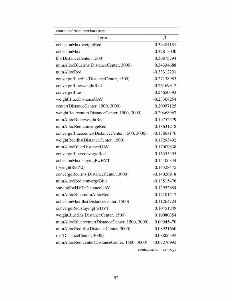
continued from previous page
Term β
cohesionMax:weightRed 0.39484181cohesionMax -0.37815030lhs(DistanceCenter, 1500) 0.36875794numAllocBlue:rhs(DistanceCenter, 3000) 0.34334688numAllocRed -0.33312201convergeBlue:lhs(DistanceCenter, 1500) -0.27138983convergeBlue:weightRed 0.26469812convergeBlue 0.24650393weightBlue:DistanceUAV -0.23308254center(DistanceCenter, 1500, 3000) 0.20957125weightRed:center(DistanceCenter, 1500, 3000) -0.20468967numAllocBlue:weightRed 0.19752579numAllocRed:convergeRed 0.18631218convergeBlue:center(DistanceCenter, 1500, 3000) -0.17804176weightRed:lhs(DistanceCenter, 1500) 0.17293492numAllocBlue:DistanceUAV 0.17009838convergeBlue:convergeRed 0.16355295cohesionMax:stayingPwHVT 0.15406344I(weightRed^2) 0.14528475convergeRed:rhs(DistanceCenter, 3000) -0.14026918numAllocRed:convergeBlue -0.13515476stayingPwHVT:DistanceUAV 0.12952884numAllocBlue:numAllocRed 0.12101517cohesionMax:lhs(DistanceCenter, 1500) -0.11264724convergeRed:stayingPwHVT 0.10451249weightBlue:lhs(DistanceCenter, 1500) 0.10080354numAllocBlue:center(DistanceCenter, 1500, 3000) 0.09945470numAllocRed:rhs(DistanceCenter, 3000) -0.08921660rhs(DistanceCenter, 3000) -0.08806592numAllocRed:center(DistanceCenter, 1500, 3000) -0.07276992
continued on next page
92

continued from previous page
Term β
stayingPwHVT:lhs(DistanceCenter, 1500) -0.07254442numAllocRed:cohesionMax -0.07117946numAllocBlue:convergeRed -0.06902416convergeBlue:DistanceUAV 0.06282924cohesionMax:center(DistanceCenter, 1500, 3000) -0.06238867cohesionMax:rhs(DistanceCenter, 3000) 0.06003309numAllocBlue:cohesionMax 0.05982500convergeBlue:rhs(DistanceCenter, 3000) -0.05889753DistanceUAV:rhs(DistanceCenter, 3000) 0.05888981cohesionMax:convergeRed -0.05425259numAllocRed:DistanceUAV 0.05360961numAllocRed:lhs(DistanceCenter, 1500) -0.05287791numAllocBlue:convergeBlue -0.05039057weightBlue:center(DistanceCenter, 1500, 3000) 0.05022147stayingPwHVT:center(DistanceCenter, 1500, 3000) -0.04688542convergeRed:center(DistanceCenter, 1500, 3000) -0.04247425convergeRed:weightBlue -0.04041143DistanceUAV:lhs(DistanceCenter, 1500) -0.04040390DistanceUAV:center(DistanceCenter, 1500, 3000) 0.02971351cohesionMax:convergeBlue 0.02934506convergeRed:DistanceUAV 0.02626016convergeBlue:stayingPwHVT -0.02441405convergeRed:lhs(DistanceCenter, 1500) -0.01687805
Table B.1: Sorted terms of the fitted model with β s.
93

THIS PAGE INTENTIONALLY LEFT BLANK
94

REFERENCES
[1] H. Geer and C. Bolkcom, “Unmanned aerial vehicles: Background and issues forCongress,” CRS Report for Congress, CRS Report No. RL31872.
[2] P. Feigin, O. Pinkas, and J. Shinar, “A simple Markov model for the analysis of multipleair combat,” Naval Research Logistics Quarterly, vol. 31, 1984.
[3] W. Nunn and R. Oberle, “Evaluating air combat maneuvering Engagements Vol. I -methodology,” Center for Naval Analyses CNS, vol. I, no. Op 03, 1976.
[4] D. Frelinger, J. Kvitky, and W. Stanley, “Proliferated autonomous weapons,” Rand Corp.,Santa Monica, CA, Tech. Rep., 1997.
[5] B. T. Clough, “UAV swarming? So what are those swarms, what are the implications,and how do we handle them?” in AUVSI Unmanned System Conf., Orlando, FL, 2002.
[6] C. W. Reynolds, “Flocks, herds and schools: A distributed behavioral model,” ACMSIGGRAPH Computer Graphics, vol. 21, no. 4, pp. 25–34, Aug. 1987.
[7] I. C. Price, “Evolving self-organized behavior for homogeneous and heterogeneous UAVor UCAV swarms,” Ph.D. dissertation, Air Force Air University, Wright-Patterson AirForce Base, OH, 2006.
[8] M. Day, “Multi-agent task negotiation among UAVs to defend against swarm attacks,”M.S. thesis, Naval Postgraduate School, Monterey, CA, 2012.
[9] B. J. Cobb, “Adaptive discrete event simulation for analysis of Harpy swarm attack,”M.S. thesis, Naval Postgraduate School, Monterey, CA, 2011.
[10] Barbara Starr, “Iranian jets fire on U.S. drone,” 2012. [Online]. Available:http://security.blogs.cnn.com/2012/11/08/first-on-cnn-iranian-jets-fire-on-u-s-drone/
[11] CNNWireStaff, “Israel shoots down drone,” 2012. [Online]. Available:http://www.cnn.com/2012/10/06/world/meast/israel-drone-downed/index.html
[12] ArmyUASCoEStaff, “Eyes of the Army–US Army Roadmap for Unmanned AircraftSystems 2010–2035,” US Army UAS Center of Excellence, 2010.
[13] R. Shaw, Fighter combat: Tactics and maneuvering. Annapolis, MD: USNI, 1985.
[14] S. Edwards, Swarming on the Battlefield: Past, Present, and Future. Santa Monica, CA:Rand Corp., 2000.
[15] T. W. Lucas and S. M. Sanchez, “Exploring the world of agent-based simulations: simplemodels, complex analyses,” in Proc. of the 2002 Winter Simulation Conf. San Diego,CA: IEEE, 2002, pp. 116–126.
95

[16] D. Nowak, “Exploitation of self organization in uav swarms for optimization in combatenvironments,” Ph.D. dissertation, Air Force Air University, Wright-Patterson Air ForceBase, OH, 2008.
[17] S. F. Railsback, S. L. Lytinen, and S. K. Jackson, “Agent-based simulation platforms:review and development recommendations,” Simulation, vol. 82, no. 9, pp. 609–623, Sep.2006.
[18] George Mason University, “MASON,” 2013. [Online]. Available:http://cs.gmu.edu/~eclab/projects/mason/
[19] T. Cioppa, T. W. Lucas, and S. M. Sanchez, “Military applications of agent-basedsimulations,” Proc. of the 2004 Winter Simulation Conf., 2004., vol. 1, pp. 165–174,2004.
[20] S. Luke, C. Cioffi-Revilla, and L. Panait, “MASON: A multiagent simulationenvironment,” Simulation, pp. 1–18, 2005.
[21] The Eclipse Foundation, “Eclipse,” 2013. [Online]. Available: http://www.eclipse.org/
[22] L. Dubins, “On curves of minimal length with a constraint on average curvature, and withprescribed initial and terminal positions and tangents,” Amer. J. of Math., vol. 79, no. 3,pp. 497–516, 1957.
[23] H. Chitsaz and S. M. LaValle, “Time-optimal paths for a Dubins airplane,” in 2007 46thIEEE Conf. on Decision and Control. New Orleans, LA: Ieee, 2007, pp. 2379–2384.
[24] S. M. Ross, Introduction to Probability Models, Tenth Edition. Burlington, MA:Academic Press, 2009.
[25] S. M. Sanchez, “Work Smarter, Not Harder: Guidelines for Designing SimulationExperiments,” in Proc. of the Winter Simulation Conf., 2005., pp. 69–82, 2005.
[26] J. P. C. Kleijnen, S. M. Sanchez, T. W. Lucas, and T. M. Cioppa, “State-of-the-art review:A user’s guide to the brave new world of designing simulation experiments,” INFORMSJ. on Computing, vol. 17, no. 3, pp. 263–289, Jul. 2005.
[27] N. Draper and D. Lin, “Capacity considerations for two-level fractional factorialdesigns,” J. of statistical planning and inference, 1990.
[28] P. J. Sanchez, “Efficient generation of resolution VII fractional factorial designs,”unpublished.
[29] S. M. Sanchez, “NOLH designs spreadsheet,” 2011. [Online]. Available:http://harvest.nps.edu/
96

[30] D. D. Wackerly, W. Mendenhall III, and R. L. Scheaffer, Mathematical Statisctics withApplications, 7th ed. Belmont, CA: Books/Cole, Cengage Learning, 2008.
[31] A. Law, Simulation Modeling and Analysis with Expertfit Software. New York, NY:McGraw-Hill Science/Engineering/Math, 2006.
[32] J. J. Faraway, Extending the Linear Model with R: Generalized Linear, Mixed Effects andNonparametric Regression Models (Chapman & Hall/CRC Texts in Statistical Science).Boca Raton, FL: Chapman and Hall/CRC, 2005.
[33] T. Hastie, R. Tibshirani, and J. Friedman, The Elements of Statistical Learning: DataMining, Inference, and Prediction, Second Edition (Springer Series in Statistics). NewYork: Springer, 2009.
[34] D. C. Montgomery and G. C. Runger, Applied Statistics and Probability for Engineers.New York: Wiley, 2010.
97

THIS PAGE INTENTIONALLY LEFT BLANK
98

Initial Distribution List
1. Dudley Knox LibraryNaval Postgraduate SchoolMonterey, California
2. Defense Technical Information CenterFt. Belvoir, Virginia
99