2015 standard scenarios annual report: u.s. electric ... · sector scenario exploration ... from...

NREL is a national laboratory of the U.S. Department of Energy Office of Energy Efficiency & Renewable Energy Operated by the Alliance for Sustainable Energy, LLC This report is available at no cost from the National Renewable Energy Laboratory (NREL) at www.nrel.gov/publications.

Contract No. DE-AC36-08GO28308

2015 Standard Scenarios Annual Report: U.S. Electric Sector Scenario Exploration Patrick Sullivan, Wesley Cole, Nate Blair, Eric Lantz, Venkat Krishnan, Trieu Mai, David Mulcahy, and Gian Porro National Renewable Energy Laboratory

Technical Report NREL/TP-6A20-64072 July 2015

NREL is a national laboratory of the U.S. Department of Energy Office of Energy Efficiency & Renewable Energy Operated by the Alliance for Sustainable Energy, LLC This report is available at no cost from the National Renewable Energy Laboratory (NREL) at www.nrel.gov/publications.

Contract No. DE-AC36-08GO28308

National Renewable Energy Laboratory 15013 Denver West Parkway Golden, CO 80401 303-275-3000 • www.nrel.gov

2015 Standard Scenarios Annual Report: U.S. Electric Sector Scenario Exploration Patrick Sullivan, Wesley Cole, Nate Blair, Eric Lantz, Venkat Krishnan, Trieu Mai, David Mulcahy, and Gian Porro National Renewable Energy Laboratory

Prepared under Task No. SA15.0110

Technical Report NREL/TP-6A20-64072 July 2015

NOTICE

This report was prepared as an account of work sponsored by an agency of the United States government. Neither the United States government nor any agency thereof, nor any of their employees, makes any warranty, express or implied, or assumes any legal liability or responsibility for the accuracy, completeness, or usefulness of any information, apparatus, product, or process disclosed, or represents that its use would not infringe privately owned rights. Reference herein to any specific commercial product, process, or service by trade name, trademark, manufacturer, or otherwise does not necessarily constitute or imply its endorsement, recommendation, or favoring by the United States government or any agency thereof. The views and opinions of authors expressed herein do not necessarily state or reflect those of the United States government or any agency thereof.

This report is available at no cost from the National Renewable Energy Laboratory (NREL) at www.nrel.gov/publications.

Available electronically at SciTech Connect http:/www.osti.gov/scitech

Available for a processing fee to U.S. Department of Energy and its contractors, in paper, from:

U.S. Department of Energy Office of Scientific and Technical Information P.O. Box 62 Oak Ridge, TN 37831-0062 OSTI http://www.osti.gov Phone: 865.576.8401 Fax: 865.576.5728 Email: [email protected]

Available for sale to the public, in paper, from:

U.S. Department of Commerce National Technical Information Service 5301 Shawnee Road Alexandria, VA 22312 NTIS http://www.ntis.gov Phone: 800.553.6847 or 703.605.6000 Fax: 703.605.6900 Email: [email protected]

Cover Photos by Dennis Schroeder: (left to right) NREL 26173, NREL 18302, NREL 19758, NREL 29642, NREL 19795.

NREL prints on paper that contains recycled content.

http://www.osti.gov/scitech

http://www.osti.gov/

mailto:[email protected]

http://www.ntis.gov/

mailto:[email protected]

iii


Preface This report is one of several products resulting from an initial effort to provide a consistent set of technology cost and performance data and to define a conceptual and consistent scenario framework that can be used in the National Renewable Energy Laboratory’s (NREL’s) future analyses. The long-term objective of this effort is to identify a range of possible futures of the U.S. electricity sector in which to consider specific energy system issues through (1) defining a set of prospective scenarios that bound ranges of key technology, market, and policy assumptions and (2) assessing these scenarios in NREL’s market models to understand the range of resulting outcomes, including energy technology deployment and production, energy prices, and carbon dioxide (CO2) emissions.

The initial effort, supported by the U.S. Department of Energy’s (DOE) Office of Energy Efficiency and Renewable Energy (EERE), focused on the electric sector by creating a technology cost and performance database, defining scenarios, documenting associated assumptions, and generating modeled results using NREL’s Regional Energy Deployment Systems (ReEDS) model. This work leverages and continues significant activity already being funded by EERE for individual technologies and market segments.

The specific products from the initial effort including the following:

• An Annual Technology Baseline (ATB) workbook documenting detailed cost and performance data (both current and projected) for both renewable and conventional technologies

• An ATB summary presentation in PowerPoint describing each of the technologies and providing additional context for their treatment in the workbook

• This 2015 Standard Scenarios Annual Report describing the identified scenarios, associated assumptions (including technology cost and performance assumptions from the ATB), modeled results, and the base structure of the specific version of the ReEDS model (v2015.1) (annual “release”) used to generate the results.

These products can be accessed at www.nrel.gov/analysis/data_tech_baseline.html.

NREL intends to consistently apply these products in its ongoing electric sector scenarios analyses to ensure that the analyses incorporate a transparent, realistic, and timely set of input assumptions and consider a diverse set of potential futures. The application of standard scenarios, clear documentation of underlying assumptions, and model versioning is expected to result in:

• Improved transparency of critical input assumptions and modeling methodologies • Improved comparability of results across studies • Improved consideration of the potential economic and environmental impacts of

generation technology improvement, changes in market conditions, and changes to policies and regulations

• An enhanced framework for formulating and addressing new analysis questions.

NREL plans to update the scenario framework and technology baseline annually and extend it to other technologies, models, and sectors, including transportation and the built environment.

http://www.nrel.gov/analysis/data_tech_baseline.html

iv


Acknowledgements We gratefully acknowledge the many people whose efforts contributed to this report. The ReEDS modeling and analysis team was active in developing and testing the ReEDS model v.2015.1. Current and past team members include Stuart Cohen, Kelly Eurek, Bethany Frew, Donna Heimiller, Eduardo Ibanez, Anthony Lopez, Andrew Martinez, Matthew Mowers, Ben Sigrin, Walter Short, Caroline Uriarte, and Owen Zinaman. We also thank the NREL technology analysts who provided input on the technology costs, assumptions, and methodologies in ReEDS: Chad Augustine, Karlynn Cory, Maureen Hand, David Feldman, Robert Margolis, and Craig Turchi. Numerous NREL colleagues reviewed and improved this report, including Doug Arent, Paul Basore, David Corbus, David Mooney, Michael Pacheco, Sarah Truitt, and Mary Werner. Robin Newmark and Bobi Garrett, especially, provided key leadership and guidance for this project. We thank the external reviewers whose insights helped us create a better product: Peter Blair, Elise Brown, Jordan Kislear, Chris Namovicz, Cristian Rabiti, Mark Reeder, Ann Satsangi, and Ryan Wiser. Some of the input data, model developments, and text were developed in a parallel effort sponsored by the DOE Wind and Water Power Technology Office. This report was funded by the DOE Office of Energy Efficiency and Renewable Energy under contract number DE-AC36-08GO28308. Any and all errors and omissions are the sole responsibility of the authors.

v


Executive Summary This report describes 19 standard scenarios projecting the evolution of the U.S. electric sector from the present through 2050 along with the base structure and assumptions for the Regional Energy Deployment System (ReEDS) model v.2015.1, which is the current tool used for running the scenarios. This work relies on the compilation of technology cost and performance assumptions presented in the NREL Annual Technology Baseline (ATB). The Standard Scenarios span an assumption space of major drivers that are likely to influence the development of the U.S. electric sector. This assumption space incorporates both inputs from the NREL ATB and the structure of the ReEDS model.

ReEDS is an electricity system capacity expansion model that develops scenarios of future investment and operation of generation and transmission capacity to meet U.S. electricity requirements (Alaska and Hawaii are not included). ReEDS scenarios are not forecasts or projections. They instead provide a framework for exploring future electricity systems while considering the potential impacts of technological development, policy changes, or economic conditions.

ReEDS has been developed with an emphasis on characteristics important to renewable electricity technologies: variability, uncertainty, geographic resource diversity and specificity, and transmission requirements. Its high spatial resolution and statistical treatment of the impact of variable wind and solar resources enable representation of the relative value of geographically and temporally heterogeneous renewable power resources. Renewable energy technologies represented in ReEDS include land-based and offshore wind power, solar photovoltaic (PV) and concentrating solar power (CSP), geothermal power, biopower, and hydropower. The technology input assumptions, sources, and treatments are also discussed in the accompanying NREL ATB workbook and PowerPoint products (NREL 2015).

Central Scenario The Central Scenario is the result of running ReEDS v.2015.1 with default settings and is therefore a useful benchmark for understanding the baseline behavior of this model version. The Central Scenario represents a dramatic transition in electricity provision in the United States (see Figure 1 and Figure 2). Load in the scenario grows through 2050, requiring growth in generating stock to meet the increases. Meanwhile, as the aging electricity fleet ReEDS begins with in 2010 retires—a third of the capacity that existed in 2010 retires before 2040, and almost half retires by the end of the model horizon in 2050—shifting economics and technology innovation lead to retiring stock being replaced by a different portfolio of technologies.

vi


Figure 1. Installed capacity by technology type in the Central Scenario. Gas-CT is gas-fired combustion turbine and Gas-CC is gas-fired combined cycle.

Figure 2. Generation by technology type in the Central Scenario. Gas-CT is gas-fired combustion turbine and Gas-CC is gas-fired combined cycle.

0

200

400

600

800

1000

1200

1400

1600

1800

2010

2012

2014

2016

2018

2020

2022

2024

2026

2028

2030

2032

2034

2036

2038

2040

2042

2044

2046

2048

2050

Cap

acity

(GW

)

Storage

Solar

Wind

Biopower

Geothermal

Hydro

Gas-CT

Gas-CC

Oil-Gas-Steam

Coal

Nuclear

0

1000

2000

3000

4000

5000

6000

2010

2012

2014

2016

2018

2020

2022

2024

2026

2028

2030

2032

2034

2036

2038

2040

2042

2044

2046

2048

2050

Gen

erat

ion

(TW

h)

Imports

Solar

Wind

Biopower

Geothermal

Hydro

Gas-CT

Gas-CC

Oil-Gas-Steam

Coal

Nuclear

vii


One clear dynamic is a shift from coal to natural gas, continuing the trend of the past decade. Persistently low natural gas prices, as assumed, keep natural gas combined cycle plants competitive, and thus increase their market share as the contributions from the coal fleet steadily decrease.

This scenario also sees substantial growth and investment in generation from renewable technologies, especially land-based wind power and PV. Installed wind capacity grows from 65 gigawatts (GW) in 2014 to nearly 300 GW in 2050, and solar expands to almost 400 GW. These trends continue recent historic growth in renewable generation, bringing the power sector from a minor (<1%) contribution from wind and solar in 2000, to nearly 6% of generation today, and on to 36% of generation in 2050.

Standard Scenarios Some of the scenarios in this ensemble involve changes in parameters generally considered influential on the evolution of the power sector: fuel prices, rate of demand growth, technological improvement, and the retirement schedule of today’s fleet. These scenarios were chosen because they can strongly influence model outcomes, and because there is significant uncertainty about how the input driver (e.g., fuel prices) will change over time. For these scenarios, we include two scenarios in the ensemble that vary in both directions from the baseline assumption in the Central Scenario. For example, for fossil fuel price assumptions we include both a high fuel price scenario and a low fuel price scenario.

Other scenarios are more individually defined, each as its own vision of the future distinct from the Central Scenario. These other scenarios are chosen either because of general growing interest in the area (e.g., carbon policy) or because the scenarios demonstrate a few ReEDS model options or capabilities that are not otherwise on display. They are included to provide context for how these options can change the model’s behavior. Table 1 summarizes all the scenarios.

viii


Table 1. Summary of the Standard Scenarios. The scenario settings listed in blue italics correspond to the setting in the Central Scenario.

Group Scenario Notes

Fossil Fuel Prices

Reference Fuel Prices AEO 2014 Natural Gas (NG) and Coal Reference

Low Fuel Prices AEO 2014 High Oil & Gas Resource, Low Coal Price

High Fuel Prices AEO 2014 Low Oil & Gas Resource, High Coal Price

Electricity Demand Growth

Reference Demand Growth AEO 2014 Reference

Low Demand Growth AEO 2014 Low Economic Growth

High Demand Growth AEO 2014 High Economic Growth

Vehicle Electrification PEV/PHEV adoption reaches 30% of sales by 2050; 45% of charging utility-controlled, 55% opportunistic

Renewable Energy Technology Costs

Mid RE Cost Annual Technology Baseline (ATB) Mid-Case Projections

Low RE Cost Annual Technology Baseline (ATB) Low-Case Projections

High RE Cost Annual Technology Baseline (ATB) High-Case Projections

RE Technology Improvement EERE program office technology cost and performance goals

Existing Fleet Retirements

Reference Retirement Generator Database and Online Year (Ventyx); Planned Coal Retirements (M.J. Bradley)

Extended Nuclear Lifetime Relicensing to 80 years

Accelerated Coal Retirement 50-year lifetime if built after 1970 (from 65+); Accelerated retirement if built before 1970

Policy/Regulatory Environment

Extended Incentives for RE Generation Extend ITC/PTC through 2030 for eligible technologies

National Renewable Portfolio Standard (RPS)

43% of generated electricity from renewables by 2030, 80% by 2050

ix



Power Sector CO2 Cap President’s Climate Goal: power sector emissions 17% below 2005 levels by 2020, 83% by 2050

Current Law Used for the Central Scenario

Earth System Feedbacks Impacts of Climate Change

Temperature impacts on generators, transmission, and load; derived from IGSM-CAM climate scenario

Resource and System Constraints

Reduced RE Resource Simple 25% cut to resource in input supply curves

Barriers to Transmission System Expansion

3x transmission capital cost No new AC-DC-AC interties 2x transmission loss factors

Restricted Cooling Water Use New construction may not use freshwater for cooling

Generation Technology Improvement

Nuclear Technology Breakthrough 40% reduction in nuclear capital costs

x


Figures 3–6 show the range of wind, solar, geothermal, and hydropower generation outputs, respectively, for the subset of the scenarios that include fuel prices, rate of demand growth, technological improvement, and the retirement schedule of today’s fleet. The range of these outputs varies considerably based on the input drivers. For example, the scenario with the highest solar generation in 2050 has five times more generation than the scenario with the least solar generation. Some of the drivers of the range have asymmetric effects across the technologies—some input variations heavily impact one technology but not another.

Figure 3. Annual wind generation in the scenarios that include bidirectional changes in fuel prices, rate of demand growth, technological improvement, and the retirement schedule of today’s

fleet. Wind generation includes land-based and offshore wind. This range of generation

corresponds to 145–379 GW of wind capacity in 2050.

0

200

400

600

800

1000

1200

1400

1600

1800

2010 2020 2030 2040 2050

Win

d G

ener

atio

n (T

Wh)

Central ScenarioLow Fuel PricesHigh Fuel PricesLow Economic GrowthHigh Economic GrowthLow Cost Solar & WindHigh Cost Solar & WindAccelerated Coal RetirementsExtended Nuclear Lifetime

xi


Figure 4. Annual solar generation in the scenarios that include bidirectional changes in fuel prices, rate of demand growth, technological improvement, and the retirement schedule of

today’s fleet. Solar generation includes CSP, distributed PV, and utility PV. This range of generation

corresponds to 142–559 GW of solar capacity in 2050.

Figure 5. Annual geothermal generation in the scenarios that include bidirectional changes in fuel prices, rate of demand growth, technological improvement, and the retirement schedule of

today’s fleet. Geothermal generation includes known hydrothermal and near-field enhanced geothermal

systems (EGS). Undiscovered hydrothermal resources and deep EGS resources are not included in the Driver Scenarios but are included in the RE Technology Improvement Scenario. This range of generation corresponds to 6.7–8.3 GW of geothermal capacity

in 2050.

0100200300400500600700800900

1000

2010 2020 2030 2040 2050

Sola

r G

ener

atio

n (T

Wh)


0

10

20

30

40

50

60

70

2010 2020 2030 2040 2050

Geo

ther

mal

Gen

erat

ion

(TW

h)


xii


Figure 6. Annual hydropower generation in the scenarios that include bidirectional changes in fuel

prices, rate of demand growth, technological improvement, and the retirement schedule of today’s fleet.

This range of generation corresponds to 84–87 GW of hydropower capacity in 2050.

Discussion and Future Work This report—the first in an annual series—captures a range of sensitivities to a suite of drivers in the electric sector. This set of scenarios utilizes a consistent set of data and assumptions. Together, they establish a baseline understanding of the electric sector today and a range of projected pathways and form the basis for new studies and analysis. The 19 scenarios identify a range based on current understanding and projections; they do not represent predictions of how the electric sector will evolve. Rather, they map out likely trajectories within which the actual pathway may occur. Additionally, this report gives a basic description of the structure and assumption of the ReEDS model v.2015.1.

This report, coupled with the NREL ATB, also provides a resource for analysts and decision makers interested in the current and future U.S. electricity system. The report and ATB will be updated annually to provide the most relevant information. For example, the DOE solar and water programs have ongoing analysis work that may inform new solar and hydropower cost projections for the 2016 release of the report. Also, while there are high, mid, and low forecasts for many technologies, there is an ongoing effort to assess the probability of attaining each forecast and working to normalize these forecasts across technologies in terms of probability of achieving them. For example, the “high cost” trajectory could be consistently 90% likely to be achieved while the “low cost” trajectory could be 25% likely to be achieved.

The electricity sector has become increasingly complex with interactions across meters (e.g., distributed generation and demand response), across sectors (e.g., plug-in hybrid electric vehicles and natural gas for other uses), and with anticipated clean energy policies (e.g., the EPA’s proposed Clean Power Plan). NREL models, including ReEDS, will continue to evolve to model these interactions effectively. For example, ongoing efforts are linking the ReEDS model with a distributed generation model (SolarDS), a natural gas supply chain model (Rice World Gas Trade Model [RWGTM]), and an economy wide model (U.S. Regional Energy Policy [USREP]).

270

280

290

300

310

320

330

340

2010 2020 2030 2040 2050

Hyd

ropo

wer

Gen

erat

ion

(TW

h)


xiii


Table of Contents 1 Introduction ........................................................................................................................................... 1 2 Model Framework ................................................................................................................................. 3 3 Central Scenario Base Assumptions ................................................................................................. 6

3.1 Descriptions of Technologies ........................................................................................................ 6 3.1.1 Renewable Energy Resources and Technologies ............................................................. 6 3.1.2 Conventional Generation Technologies ......................................................................... 15 3.1.3 Storage and Demand-side Technologies ........................................................................ 20 3.1.4 Transmission .................................................................................................................. 21

3.2 Electricity System Operation and Reliability .............................................................................. 25 3.2.1 Electricity Load .............................................................................................................. 25

3.3 Capital Financing, System Cost, and Electricity Rates ............................................................... 30 3.3.1 Financing of Capital Stock ............................................................................................. 30 3.3.2 Calculating Total System Cost ....................................................................................... 32 3.3.3 Estimating Retail Electricity Rates................................................................................. 32

4 Central Scenario Results ................................................................................................................... 34 5 Standard Scenarios Ensemble .......................................................................................................... 38

5.1 Fossil Fuel Prices ........................................................................................................................ 40 5.2 Demand Growth .......................................................................................................................... 40 5.3 Renewable Energy Technology Costs ......................................................................................... 41 5.4 Existing Fleet Retirements .......................................................................................................... 43 5.5 Range of Outcomes among the Bidirectional Scenarios ............................................................. 44

5.5.1 Wind Generation ............................................................................................................ 44 5.5.2 Solar Generation ............................................................................................................. 45 5.5.3 Geothermal Generation .................................................................................................. 46 5.5.4 Hydropower Generation ................................................................................................. 46 5.5.5 Natural Gas Generation .................................................................................................. 47 5.5.6 Carbon Dioxide Emissions ............................................................................................. 48 5.5.7 Transmission Builds ....................................................................................................... 48 5.5.8 Electricity Prices ............................................................................................................ 49

5.6 Vehicle Electrification ................................................................................................................. 49 5.7 Extended Incentives for Renewable Energy Generation ............................................................. 51 5.8 National Renewable Portfolio Standard ...................................................................................... 52 5.9 Power Sector CO2 Cap ................................................................................................................ 53 5.10 Impacts of Climate Change ......................................................................................................... 54 5.11 Reduced RE Resource ................................................................................................................. 55 5.12 Barriers to Transmission System Expansion ............................................................................... 56 5.13 Restrictions on Thermoelectric Water Use.................................................................................. 57 5.14 Renewable Energy Technology Improvement ............................................................................ 58 5.15 Nuclear Technology Breakthrough ............................................................................................. 60

6 Discussion and Future Work ............................................................................................................. 62 References ................................................................................................................................................. 63 Appendix: Additional Scenario Output Plots ......................................................................................... 67

xiv


List of Figures Figure 1. Installed capacity by technology type in the Central Scenario. ............................................. vi Figure 2. Generation by technology type in the Central Scenario. ........................................................ vi Figure 3. Annual wind generation in the scenarios that include bidirectional changes in fuel prices,

rate of demand growth, technological improvement, and the retirement schedule of today’s fleet. ............................................................................................................................................... x

Figure 4. Annual solar generation in the scenarios that include bidirectional changes in fuel prices, rate of demand growth, technological improvement, and the retirement schedule of today’s fleet. .............................................................................................................................................. xi

Figure 5. Annual geothermal generation in the scenarios that include bidirectional changes in fuel prices, rate of demand growth, technological improvement, and the retirement schedule of today’s fleet. ................................................................................................................................. xi

Figure 6. Annual hydropower generation in the scenarios that include bidirectional changes in fuel prices, rate of demand growth, technological improvement, and the retirement schedule of today’s fleet. ................................................................................................................................ xii

Figure 7. Map showing the ReEDS regional structure. .......................................................................... 3 Figure 8. Prescribed distributed PV deployment used in the Central Scenario as determined by

SolarDS ....................................................................................................................................... 10 Figure 9. National capital cost supply curves for new identified hydrothermal and near-field EGS

capacity used in the base model assumptions ............................................................................. 13 Figure 10. National capital cost supply curve for new hydropower capacity....................................... 14 Figure 11. Base fuel price assumptions ................................................................................................ 19 Figure 12. Existing long-distance transmission infrastructure as represented in ReEDS .................... 21 Figure 13. Map of long-distance transmission costs ............................................................................ 24 Figure 14. Map of spur-line transmission costs .................................................................................... 24 Figure 15. Cumulative installed capacity by technology type in the Central Scenario ........................ 34 Figure 16. Generation by technology in each solve year in the Central Scenario ................................ 35 Figure 17. Transition from coal to natural gas, past, present, and future ............................................ 35 Figure 18. Growth in wind and solar generation, past, present, and future ......................................... 35 Figure 19. Generation by time-slice in 2010 in the Central Scenario .................................................. 36 Figure 20. Generation by time-slice in 2050 in the Central Scenario .................................................. 37 Figure 21. Carbon intensity of the electricity system (direct emissions) ............................................. 37 Figure 22. Alternate natural gas and coal price scenarios .................................................................... 40 Figure 23. Alternate load pathways ...................................................................................................... 41 Figure 24. High, medium, and low overnight capital cost trajectories for TRG 2 land-based wind

generators. ................................................................................................................................... 41 Figure 25. High, medium, and low overnight capital cost trajectories for TRG 2 offshore wind

generators. ................................................................................................................................... 42 Figure 26. High, medium, and low overnight capital costs for UPV. .................................................. 42 Figure 27. High, medium, and low overnight capital costs for CSP with 6 hours of TES. .................. 43 Figure 28. Nuclear and Coal Retirement Pathways .............................................................................. 44 Figure 29. Annual wind generation in the bidirectional scenarios. ...................................................... 45 Figure 30. Annual solar generation in the bidirectional scenarios. ...................................................... 45 Figure 31. Annual geothermal generation in the bidirectional scenarios. ............................................ 46 Figure 32. Annual hydropower generation in the bidirectional scenarios. ........................................... 47 Figure 33. Annual natural-gas-fired generation in the bidirectional scenarios..................................... 47 Figure 34. Annual CO2 emissions from the power sector in the bidirectional scenarios ..................... 48 Figure 35. Cumulative AC transmission capacity in the bidirectional scenarios ................................. 49 Figure 36. Retail electricity prices in the bidirectional scenarios ......................................................... 49 Figure 37. Vehicle Electrification Scenario ......................................................................................... 50

xv


Figure 38. Electricity generation by generator type in 2050 for the High PHEV Adoption Scenario. 51 Figure 39. Annual electricity generation by technology type............................................................... 52 Figure 40. Generation in 2050 by generator type for the 80% National RPS Scenario and the Central

Scenario ....................................................................................................................................... 53 Figure 41. Comparison of prescribed electric sector CO2 cap to the CO2 emissions path in the Central

Scenario ....................................................................................................................................... 53 Figure 42. Electricity generation over time by generator type for the Power Sector CO2 Cap Scenario54 Figure 43. Solar Generation in the Central Scenario and the Impacts of Climate Change Scenario.... 55 Figure 44. Total renewable energy generation for the Central Scenario and the Reduced RE Resource

Scenario ....................................................................................................................................... 56 Figure 45. Change in 2050 RE generation in the Reduced RE resource compared to the Central

Scenario. ...................................................................................................................................... 56 Figure 46. AC transmission capacity in the Central Scenario and the Barriers to High Transmission

Expansion Scenario ..................................................................................................................... 57 Figure 47. Cumulative water access purchases for the Central Scenario (left) and the Restrictions on

Thermoelectric Water Use (right). .............................................................................................. 58 Figure 48. Comparison of "Base" and "Improved" geothermal resource supply curves. ..................... 59 Figure 49. Renewable energy generation and CO2 emissions in the Central Scenario and the RE

Technology Improvement Scenario. ........................................................................................... 59 Figure 50. Nuclear capital cost options ................................................................................................ 60 Figure 51. Amount of electricity generation displaced by nuclear units compared to the Central

Scenario. ...................................................................................................................................... 61 Figure 52. Annual wind generation in the non-bidirectional scenarios ................................................ 67 Figure 53. Annual solar generation in the non-bidirectional scenarios. ............................................... 67 Figure 54. Annual geothermal generation in the non-bidirectional scenarios. ..................................... 68 Figure 55. Annual hydropower generation in the non-bidirectional scenarios..................................... 68 Figure 56. Annual natural-gas-fired generation in the non-bidirectional scenarios ............................. 69 Figure 57. Annual nuclear generation in the non-bidirectional scenarios ............................................ 69 Figure 58. Annual CO2 emissions from the power sector in the non-bidirectional scenarios .............. 70 Figure 59. Cumulative AC transmission capacity in the non-bidirectional scenarios .......................... 70 Figure 60. Retail electricity prices in the non-bidirectional scenarios ................................................. 71

xvi


List of Tables Table 1. Summary of the Standard Scenarios...................................................................................... viii Table 2. Definition of ReEDS Time-Slice.............................................................................................. 4 Table 3. Cost and Performance Assumptions for Land-Based Wind Technology (2013$) ................... 7 Table 4. Cost and Performance Assumptions for Offshore Wind Technologies (2013$) ...................... 8 Table 5. Cost Assumptions for Utility-Scale PV Technologies (2013$) .............................................. 10 Table 6. Characteristics of CSP Technology Storage Options ............................................................. 11 Table 7. Capacity Factor Groups for Concentrating Solar Power using a Solar Multiple of 1.4 ......... 11 Table 8. Cost Assumptions for CSP Technologies ............................................................................... 12 Table 9. Overnight Capital Cost for Conventional Generating Technologies (2013$) ........................ 17 Table 10. Operations and Maintenance Costs and Heat Rates for Conventional Generating

Technologies (2013$) .................................................................................................................. 17 Table 11. Multipliers Applied to Full-Load Heat Rates to Approximate Heat Rates for Part-

Load Operation ............................................................................................................................ 18 Table 12. Effective State RPS requirements in ReEDS ....................................................................... 29 Table 13. State Tax Incentives included in the Central Scenario ......................................................... 30 Table 14. Key Financial Assumptions .................................................................................................. 31 Table 15. Summary of the Standard Scenarios..................................................................................... 38

1


1 Introduction This report describes an ensemble of future energy system scenarios, which we call the Standard Scenarios. The scenarios span an assumption space representing a range of trajectories for major drivers of energy system development. This work relies on the National Renewable Energy Laboratory (NREL) Annual Technology Baseline (ATB), which is a compilation of technology cost and performance data for most of the technologies modeled in the scenarios. In conjunction with the assumptions in the ATB, this report describes the base structure and assumptions for the Regional Energy Deployment System (ReEDS) model v.2015.1, the version of the ReEDS electricity system model used for modeling the Standard Scenarios. This report is not a complete documentation of ReEDS, though it does describe much of the model structure and assumptions to inform the results of the Standard Scenarios. ReEDS is one of several models that NREL uses to examine future energy scenarios. Other models include SEDS (Stochastic Energy Deployment System), SolarDS (Solar Deployment System for distributed photovoltaics (PV), RPM (Resource Planning Model), and other non-electric sector models. In future years, we hope to implement similar standard scenarios in these and other models.

The results of any scenarios regarding the future of the U.S. electric sector are as much about the underlying model that is used as they are about the cost and performance inputs. The structure of the model impacts the results, such as how the model handles the variability of the renewable energy resource, the treatment of transmission and transmission growth, any intrinsic assumptions about capacity value of technologies, and any “foresight” that the model gives to the industry to adapt and adjust. NREL and other organizations have previously compared various models using both native assumptions as well as aligned input assumptions previously (Blair et al. 2009). While aligning inputs improved the alignment of the outputs, the models still did not give the same answers due to their intrinsic assumptions. To provide adequate background to inform the interpretation of the scenario results, we have included significant information in Sections 2 and 3 regarding ReEDS structure and intrinsic assumptions as well as input assumptions not represented in the ATB effort.

ReEDS is an electricity system capacity expansion model that develops scenarios of future investment and operation of generation and transmission capacity to meet U.S. electricity requirements. The model relies on system-wide, least-cost optimization to provide estimates of the type and location of fossil, nuclear, renewable, and storage resource development; the transmission infrastructure expansion requirements of those installations; and the generator dispatch and fuel needed to satisfy regional demand requirements and to maintain grid system adequacy. The model also considers technology, resource, and policy constraints, including state renewable portfolio standards. ReEDS models scenarios of the continental U.S. electricity system in two-year increments from 2010 to 2050. Although ReEDS scenarios are not forecasts or projections, they provide a framework for exploring internally consistent future electricity systems and for considering the potential impacts of technological development, policy changes, or economic conditions.

ReEDS has been developed with an emphasis on characteristics important to renewable electricity technologies: variability, uncertainty, geographic resource specificity, and transmission. Its high spatial resolution and statistical treatment of the impact of variable wind and solar resources enable representation of the relative value of geographically and temporally

2


heterogeneous renewable power resources. While the emphasis is on renewable technologies, ReEDS includes a full suite of conventional generating technologies, a system dispatch that reveals seasonal and diurnal load shapes, a reduced transmission network, and dynamic capabilities for fuel supplies and electricity load. Additional detail on the above features is included in the model description in Section 2.

While ReEDS represents many aspects of the U.S. electric system, it— like any model—has certain key limitations:1

• ReEDS is a system-wide optimization model and, therefore, does not consider revenue impacts for individual project developers, utilities, or other industry participants.

• ReEDS does not explicitly model constraints associated with the manufacturing sector. All technologies are assumed to be available at their defined capital cost in any quantity up to their technical resource potential. Penalties for rapid growth are applied in ReEDS; however, these do not fully consider all potential manufacturing or deployment limits.

• Technology cost reductions from manufacturing economies of scale and “learning by doing” are not endogenously modeled for this analysis; rather, current and future cost reduction trajectories are defined as inputs to the model.

• ReEDS has limited market foresight and, with the exception of future fuel prices, does not make decisions based on expectations of future market conditions. The model is deterministic and has limited considerations for risk and uncertainty.

• The optimization algorithm in ReEDS does not fully represent the prospecting, permitting, or siting hurdles that project developers face for either electricity generation capacity or transmission infrastructure. In other words, site-specific challenges of building electricity infrastructure are not fully captured within the model.2

• ReEDS models the power system of the continental United States, and it does not represent the broader U.S. or global energy economy. For example, competing uses of resources across sectors (e.g., natural gas) are not dynamically represented in ReEDS, and end-use electricity demand is exogenously input into ReEDS.

The remainder of this report is organized to first lay the modeling framework and assumptions for the ReEDS model (Sections 2 and 3). Section 4 describes the Central Scenario and associated assumptions for that scenario. Section 5 then presents the Standard Scenarios and the resulting impacts on the electric sector. Finally, Section 6 summarizes the work and gives some future directions.

1 Section 6 describes future work for model improvement. 2 As a linear optimization model, ReEDS also likely underestimates transmission needs due to the “lumpiness” of real transmission investments and the non-direct paths in real transmission lines compared to the point-to-point model paths.

3


2 Model Framework To determine competition between the many electricity generation, storage, and transmission options throughout the contiguous United States, ReEDS chooses the cost-optimal mix of technologies that meet regional electric power demand requirements, based on grid reliability (reserve) requirements, technology resource constraints, and policy constraints. This cost minimization routine is performed for each of 21 two-year periods from 2010 to 2050. Some of the major outputs of ReEDS include the amount and location of generator capacity and annual generation from each technology, storage capacity expansion, transmission capacity expansion, total electric sector costs, electricity price, fuel demand and prices, and carbon dioxide (CO2) emissions.

Within ReEDS, load is served and power plants are constructed in 134 balancing areas (BAs) that overlay the continental United States, shown in Figure 7. The model’s transmission network connects those BAs and comprises roughly 300 representative lines across the three asynchronous interconnections—Western, Eastern, and ERCOT. The BAs also respect state boundaries, allowing the model to represent individual state regulations and incentives. Additional geographical layers include 18 model regional transmission operators (RTOs) designed after existing RTOs, independent system operator (ISO) regions and other regions; 13 North American Electric Reliability Corporation (NERC) regions; and 9 census regions. The 13 NERC regions and 9 census regions are used to define load growth and fuel price inputs from the U.S. Energy Information Administration (EIA) and the National Energy Modeling System (NEMS). The BAs are also subdivided into 356 resource regions that describe wind and solar resource supply and quantity.

Figure 7. Map showing the ReEDS regional structure.

ReEDS includes 3 interconnections, 134 balancing areas, and 356 wind and CSP resource regions.

4


Table 2. Definition of ReEDS Time-Slice

Time-slice Number of hours per year Season Time of Day Time Period

H1 736 Summer Overnight 10 p.m. 6 a.m.

H2 644 Summer Morning 6 a.m. 1 p.m.

H3 328 Summer Afternoon 1 p.m. 5 p.m.

H4 460 Summer Evening 5 p.m. 10 p.m.

H5 488 Fall Overnight 10 p.m. 6 a.m.

H6 427 Fall Morning 6 a.m. 1 p.m.

H7 244 Fall Afternoon 1 p.m. 5 p.m.

H8 305 Fall Evening 5 p.m. 10 p.m.

H9 960 Winter Overnight 10 p.m. 6 a.m.

H10 840 Winter Morning 6 a.m. 1 p.m.

H11 480 Winter Afternoon 1 p.m. 5 p.m.

H12 600 Winter Evening 5 p.m. 10 p.m.

H13 736 Spring Overnight 10 p.m. 6 a.m.

H14 644 Spring Morning 6 a.m. 1 p.m.

H15 368 Spring Afternoon 1 p.m. 5 p.m.

H16 460 Spring Evening 5 p.m. 10 p.m.

H17 40 Summer Peak 40 highest demand hours of H3

ReEDS serves load and maintains operational reliability over 17 time-slices in each solve year, defined in Table 2. Each of the four seasons is modeled as a representative day of four time-slices: overnight, morning, afternoon, and evening. The 17th time-slice is a summer “superpeak” representing the top 40 hours of summer load. While this schedule does allow the model to capture seasonal and diurnal variations in demand, wind, and solar profiles, it is insufficient to address some of the shorter timescale challenges associated with high variable generation penetration. To more accurately represent how renewable grid integration might affect investment and dispatch decisions, the ReEDS model includes statistical parameters designed to address variability and uncertainty of wind and certain other renewable resources. These parameters include capacity value for system adequacy, forecast error reserve requirements, and curtailment estimates. The three “variability parameters” are each discussed in-depth in Section 3.2.

The major conventional thermal generating technologies included in ReEDS include simple and combined cycle natural gas, several varieties of coal, oil/gas steam, and nuclear. On top of those, ReEDS includes many renewable technologies using several kinds of resources, including geothermal, hydropower, biopower, wind, and solar. Electricity storage technologies include pumped-hydropower storage (PHS), compressed-air energy storage (CAES), batteries, and CSP with thermal storage. Included technologies are discussed in Section 3, including the parameters by which they are characterized in the model and the sources of those parameters. The objective

5


is for ReEDS to account for fundamental differences across technologies, for instance, differences in fuel cost, efficiency, or operational flexibility.

With a system-wide central-planner perspective, ReEDS is not designed to evaluate distributed generation adoption decisions. For this reason, the ReEDS analysis is supported by the SolarDS model (Denholm, Margolis, and Drury 2009). SolarDS is an adoption/diffusion model well suited to producing scenarios of market uptake of distributed PV. ReEDS takes as input SolarDS adoption scenarios produced with storylines (i.e., PV module prices and electricity rates) that are consistent across models.

ReEDS is structured as a sequence of 21 individual, but interacting,3 optimization problems, each representing a two-year period from 2010 to 2050. Each ReEDS scenario launches with an infrastructure base representing installed generation and transmission capacity as of January 1, 2009. New infrastructure that came online from 2009 through the present is prescribed into the ReEDS system in the proper solve year, and recently decommissioned units are removed in the same way. Similarly, high-likelihood, pending generators are included as prescribed builds in near-term future years, and scheduled retirements are set to be removed from the fleet as appropriate. Additionally, ReEDS inputs include an equipment lifetime for each technology that is used to retire capacity as it ages out. In certain types of scenarios, some existing stock can be underutilized due, for example, to high fuel prices or emissions standards. ReEDS facilitates “economic” retirements of underutilized coal generators if their usage falls below a certain threshold.

ReEDS tracks emissions of CO2, sulfur dioxide (SO2), nitrogen oxides (NOx), and mercury from both generators and storage technologies. Caps can be imposed at the national level on any of these emissions, and constraints can be applied to impose caps at state or regional levels. Applying a carbon tax instead of a cap is another option; the tax level and ramp-in pattern can be defined exogenously.

Annual electric loads and fuel price supply curves are exogenously specified to define the system boundaries for each period of the optimization. The source for most load and fuel inputs is the most recent Annual Energy Outlook (AEO).4 Coal and uranium fuels are assumed to be price-inelastic; ReEDS can demand as much of those fuels as it likes at the AEO-specified price. However, natural gas prices are defined by regional supply curves so that the prices respond to changes in demand.

3 Because ReEDS is a sequential model, it is path dependent, so that solutions in a given solve period inform the starting point of the next optimization year. 4 Any inputs to ReEDS v.2015.1 from AEO are sourced from the 2014 edition of the AEO (EIA 2014) or its Assumptions (EIA 2014a) unless otherwise specified.

6


3 Central Scenario Base Assumptions 3.1 Descriptions of Technologies 3.1.1 Renewable Energy Resources and Technologies One of the primary focus areas for the ReEDS model is renewable energy technologies. For that reason, renewables are characterized in detail in the model. This characterization encompasses resource assessments, projected technology improvement, interconnection costs, and operational implications of integration. Technologies include are land-based and offshore wind power, solar photovoltaic (PV) and concentrating solar power (CSP),5 geothermal, biopower, and hydropower. The input assumptions, sources, and treatments are discussed in the following sections. Transmission considerations for renewable energy technologies are discussed in Section 3.1.4.

Where given in the sections below, renewable energy resource potential values refer to the resource potential represented in ReEDS and not the total technical resource potential. The renewable potential capacity modeled in ReEDS includes cutoffs in the pre-processing steps for the model, such as assumed transmission access limits or a narrower set of technologies considered.6

3.1.1.1 Land-Based Wind Wind technology input assumptions for Central Scenario are grounded in historical trends and published projections of future wind technology cost and performance. They assume continued technology development, optimization, and maturation. Present land-based wind assumptions are based on reported costs (e.g., (Wiser and Bolinger 2013)) and modeled performance of currently available technology (e.g., (Wiser et al. 2012)). Projections of future cost and performance are derived from a review and analysis of independent literature projections (see also (Lantz, Wiser, and Hand 2012) and (Tegen et al. 2012)).

Wind turbine models can be classified into three different International Electrotechnical Commission (IEC) turbine ratings (I–III), designed for a range of annual average wind speeds.7 The Class I turbines have smaller rotors relative to the size of the generator, or a higher specific power (watts per meter squared, or W/m2), and are therefore rated to withstand higher winds. In the lowest wind resources, Class III turbines are primarily used to gain the highest capacity factor possible in lower wind speeds. Interpolating cost and performance across the three IEC classes allows monotonic functions of cost and performance by annual average wind speed. Central Scenario cost and performance assumptions for land-based wind plants are based on expected cost and performance for a turbine (representative or interpolated) appropriate for the average annual wind speed at the site.

5 CSP refers to solar thermal power and not concentrating PV. 6 Lopez et al. (2012) present renewable technical potential for the United States. 7 IEC Class I turbines are used with an annual average wind speeds of 10 meters/second (m/s) and higher; IEC Class III are used with an annual average wind speed of 7.5 m/s and lower. A blend of Class II and Class III turbines are used at annual average wind speeds of 7.5–8.5 m/s; while a blend of Class II and Class I turbines are used at annual average wind speeds of 8.5–10 m/s.

7


The resource assessment for land-based wind starts with a resource map of hourly wind speeds for the United States and offshore areas (for offshore, see Section 3.1.1.2). Land area is filtered to exclude a standard set of areas considered unlikely to be developed for environmental or technical reasons: federal and state protected areas (parks, wilderness areas, wildlife sanctuaries, etc.), areas covered by water, urban areas, wetlands, airports, and rough terrain. Non-ridge-crest forest, non-ridge-crest U.S. Forest Service and Department of Defense lands, and state forests (where available in geographic information systems [GIS]) are 50% excluded. Lower wind-speed areas are also ignored, on economic grounds. The remaining resource totals more than 6,000 gigawatts (GW).

Wind sites are grouped into five resource classes (a.k.a., techno-resource groups or TRGs) for ReEDS, based on estimated levelized cost of energy (LCOE) for present-day technology. Each class includes representative costs and expected output, shown in Table 3, along with cost and performance improvements over time.

Table 3. Cost and Performance Assumptions for Land-Based Wind Technology (2013$) Overnight Capital Cost

($/ kW) Fixed Operations and Maintenance ($/kW/ yr)

Net Capacity Factor (%)

2014 2030 2050 2014 2030 2050 2014 2030 2050

TRG 1 1,641 1,518 1,512 51 47 46 51 57 60

TRG 2 1,641 1,518 1,512 51 47 46 47 52 55

TRG 3 1,729 1,724 1,625 51 47 46 44 50 53

TRG 4 1,758 1,724 1,722 51 47 46 38 44 47

TRG 5 1,758 1,724 1,722 51 47 46 32 37 40

3.1.1.2 Offshore Wind There is substantial diversity in offshore wind generators, in terms of distance from shore, water depth, and resource quality. ReEDS subdivides offshore wind potential into ten resource classes: four for shallow resource and three each for mid-depth and deep-water resource. The depth categories correspond to turbine mounting and anchoring technologies. The shallow resource (0–30 m) is accessible via current monopile foundations; mid-depth resource (30–60 m) is expected to be accessible to jacket (truss-style) foundations; and deep-water resource (60–700 m) sites are expected to be feasible only for floating anchorage. Within each depth category, the classes are distinguished by resource quality, and then cost supply curves differentiate resource by cost of accessing transmission.

Eligible offshore area for wind development includes open water within the U.S.-exclusive economic zone with water depth less than 700 m, including the Great Lakes. As with land-based resource, offshore zones are filtered to remove areas considered unsuitable for development including national marine sanctuaries, marine protected areas, wildlife refuges, shipping and towing lanes, offshore platforms, and ocean pipelines. More than 1,500 GW of technical offshore wind potential remains after applying the exclusions.

8


Starting-point cost data are derived from the published data of the global offshore wind industry as well as estimates from recent development activity on the Atlantic Coast of the United States (Tegen et al. 2012). These data are coupled with engineering assessments and distance-based cost functions (specific to the offshore export cable and incremental construction cost associated with moving farther from shore) to determine expected site-specific costs for technology across a broad range of water depths and distances from shore.

Cost reductions over time are based on improving technology and industry learning, predicated on continued offshore wind investment. Present and future cost and performance assumptions are shown in Table 4.

Table 4. Cost and Performance Assumptions for Offshore Wind Technologies (2013$) (S = shallow, M = mid-depth, D = deep)

Overnight Capital Cost ($/ kW)

Fixed Operations and Maintenance ($/kW/ yr)

Net Capacity Factor (%)

2014 2030 2050 2014 2030 2050 2014 2030 2050

S-TRG 1 5,307 3,851 3,629 132 102 99 47 52 53

S-TRG 2 5,307 3,851 3,629 132 102 99 44 48 49

S-TRG 3 5,307 3,851 3,629 132 102 99 40 44 45

S-TRG 4 5,307 3,851 3,629 132 102 99 34 37 38

M-TRG 1 5,859 4,249 4,003 132 102 99 47 51 53

M-TRG 2 5,859 4,249 4,003 132 102 99 44 48 49

M-TRG 3 5,859 4,249 4,003 132 102 99 42 46 47

D-TRG 1 6,859 4,969 4,680 162 125 122 49 54 55

D-TRG 2 6,859 4,969 4,680 162 125 122 47 51 53

D-TRG 3 6,859 4,969 4,680 162 125 122 44 48 49

3.1.1.3 Solar Photovoltaic8 ReEDS classifies three solar photovoltaic technologies: central utility-scale (UPV), distributed utility (DUPV), and rooftop. UPV and DUPV investments are evaluated directly in ReEDS,

8 Since the draft version of this product was posted, current and projected overnight capital cost values for the ATB mid-case Solar PV projection have been modified downward to reflect the significant change in solar market prices that has occurred over the last year. The 2014 overnight capital cost for utility-scale PV has been lowered to $1.90/W (in 2015$), a 20% reduction from the earlier draft, to be in line with the most recent quarterly solar market report available. In turn, these lower costs in 2014 have increased our confidence that the SunShot target of $1.00/W will be achieved earlier. As such, the mid-case projection reduces the 2014 cost to $1.50/W by 2020 (same as earlier draft), and assumes the SunShot target is reached by 2030 instead of 2040 previously (reducing projected costs beyond 2020 by 10-20% from the earlier draft). The Standard Scenarios that utilize this Solar PV mid-case projection have been rerun to develop new deployment projections. In these cases, solar capacity and generation generally increase in the mid- to long-term compared to the earlier draft, while gas and wind generation decrease.

9


while rooftop PV deployment and performance are exogenously input into ReEDS from the SolarDS model (Denholm, Margolis, and Drury 2009).

Central UPV in ReEDS represents utility-scale single-axis-tracking PV systems with a representative size of 100 megawatts (MW). Because the technical potential for UPV is so large (153,000 GW, according to (Lopez et al. 2012), UPV resource is not restricted in ReEDS. Resource supply curves that put limits on the total technical potential for UPV and DUPV are under development and will be included in future versions of ReEDS. Distributed wholesale utility-scale PV (DUPV) in ReEDS represents utility-scale single-axis-tracking systems that have a representative size of 10 MW, have an array density of 29 MW/km2, and are located within and directly connected to distribution networks. DUPV penetration in a BA is limited to 15% of the peak demand for that BA.

Compared to the large-scale, remote UPV systems, the DUPV systems have lower infrastructure requirements; we assume they connect to existing distribution substations at 13 kilovolts (kV), whereas the representative UPV system connects to a high-voltage bus at 230 kV and may require a spur line several miles long to get there. The cost of the spur line will be added in future ReEDS versions using an accessibility supply curve (Section 3.1.1.8), but the additional transformers and power electronics associated with the larger systems and higher-voltage interconnections add cost and losses to the UPV systems. On the other hand, the larger UPV systems benefit from economies of scale. On balance, we assume a per-kW cost differential of 8.5%, and we assume 5.3% more delivered energy.

Performance characteristics for UPV and DUPV are developed using NREL’s System Advisor Model (SAM) (NREL 2010) using annual hourly weather files from the National Solar Radiation Database (NSRDB) for 939 sites throughout the contiguous United States from 1998 to 2005. The representative PV capacity factor for each model BA reflects the site within each BA with the highest annual average capacity factor. No changes or improvements in capacity factor are assumed for utility-scale PV. For each site, generation profiles are averaged across the eight-year period. In this way, each BA and resource class obtains its own output profile by time-slice. ReEDS assumes all power generated by both DUPV and rooftop PV systems is consumed locally rather than being allowed to be transmitted to neighboring BAs. UPV-generated electricity, in contrast, is allowed to travel.

Solar power technology capital costs are benchmarked to cost data reported by Feldman et al. (2014) and GTM/SEIA (2015). Baseline capital cost projections from the base year to 2020 are aligned with the DOE 62.5% reduction scenario (from 2010) documented by the U.S. Department of Energy (DOE) SunShot Vision (DOE 2012). After 2020, costs decline linearly to reach the DOE 75% reduction scenario (DOE 2012) by 2030. Performance for all solar technologies varies regionally and is based on solar irradiance data from the NSRDB. Table 5 presents the capital and operations and maintenance (O&M) cost assumptions over the model horizon for utility-scale PV.

10


Table 5. Cost Assumptions for Utility-Scale PV Technologies (2013$) Cost type 2010 2013 2015 2020 2025 2030 2035 2040 2045 2050

Capital Cost ($/kWDC)

4,346 2,587 1,951 1,604 1,337 1,069 1,069 1,069 1,069 1,069

Fixed O&M ($/kWDC-yr)

21.73 18.47 16.30 7.61 7.61 7.61 7.61 7.61 7.61 7.61

Variable O&M ($/MWh)

- - - - - - - - - -

Rooftop PV includes commercial, industrial, and residential systems. SolarDS (Denholm, Margolis, and Drury 2009), a capacity expansion model for the continental U.S. rooftop market, is used to develop a future scenario for rooftop PV capacity. The base SolarDS scenario used in the Central Scenario is the 62.5% cost reduction scenario from the SunShot Vision Study. The adoption pathway is a steady increase in rooftop PV deployment through 2040 and a gradual plateau around 130 GW. Another higher adoption rooftop PV scenario is also included as an option for scenario analysis where 240 GW by 2050 are achieved.9 Figure 8 shows the capacity trajectory for rooftop PV in the base SolarDS scenario.

Figure 8. Prescribed distributed PV deployment used in the Central Scenario as determined by SolarDS

Degradation of the efficiency of solar PV capacity over time is also modeled at 0.5%/year (Jordan and Kurtz 2013). This degradation is modeled by reducing the capacity of PV that generates energy by 0.5%/year.

9 The reason for selecting the 130 GW scenario as the base is that SolarDS and ReEDS do not—at this point—communicate about PV curtailments. In the higher adoption rooftop PV scenarios that SolarDS, ReEDS curtails much of the production from rooftop PV systems built in the 2040s in certain regions, but SolarDS continues to prescribe more adoption because it does not get that feedback. A revised SolarDS is under development that will interface more closely with ReEDS; scenarios from that revised model will replace the 130-GW scenario when they become available.

0

20

40

60

80

100

120

140

2010 2020 2030 2040 2050

Dis

trib

uted

PV

Dep

loym

ent

(GW

)

11


3.1.1.4 Concentrating Solar Power Concentrating solar power (CSP) technology options in ReEDS encompass a subset of possible thermal system configurations, with and without thermal storage, as shown in Table 6. The two system types access the same resource potential, which is divided into five resource classes based on direct normal insolation (DNI) (Table 7).

Table 6. Characteristics of CSP Technology Storage Options System Configuration Dispatchability Capacity Value Curtailments

No storage Solar multiple 1.4 Insolation-dependent

Variable/ Statistical

Statistical

With storage

6–12 hours storage, solar multiple 1.6–2.7

Dispatchable Firm None

The CSP resource classes are defined by power density of DNI, developable land area having been filtered based on land cover type, slope, and protected status. CSP resource in each resource region is therefore represented as a supply curve of MW of solar collector potential, assuming a heliostat density of 62 MW/km2. Performance for each CSP resource class was developed using typical DNI year (TDY) hourly resource data (Habte et al. 2014) from representative sites of each resource region. The TDY weather files are processed through the CSP modules of SAM to develop performance characteristics for each CSP resource class and representative CSP system considered in ReEDS.

Table 7. Capacity Factor Groups for Concentrating Solar Power using a Solar Multiple of 1.4 Resource Class

DNI range: kWh/m2/day

Average Group Net CF (2010)a

Class 1 5–6.25 0.315

Class 2 6.25–7.25 0.393

Class 3 7.25–7.5 0.428

Class 4 7.5–7.75 0.434

Class 5 > 7.75 0.448 a Net capacity factor (CF) computed via System Advisor Model simulations

The representative CSP system without storage in ReEDS is a 100-MW trough system with a solar multiple of 1.4. As CSP systems without storage are non-dispatchable, output capacity factors are defined directly from SAM results. The average annual capacity factors for the solar fields of these systems range from 20% (Class 1 resource) to 31% (Class 5 resource).

The representative system for CSP with storage is a trough-based configuration and switches to a tower-based configuration in 202510 with a molten salt heat transfer fluid and a thermal storage tank between the heliostat array and the steam turbine. ReEDS has some freedom to select the

10 This transition from troughs to towers is representative only and is not an indication of expected or predicted technology adoption. In reality, multiple system configurations will likely be deployed. The year of this representative transition can be changed by a user.

12


sizes of the power block and storage reservoir for a CSP-with-storage system. Higher solar multiples result in higher annual average capacity factors, and more storage allow the systems to be more flexible, although both options increase capital costs per kilowatt of installed turbine capacity. Limitations on system configurations are selected to ensure the systems can be assumed to be fully dispatchable within the energy limitations imposed by solar multiples, hours of thermal storage, the time-profile of the solar insolation, and minimum loading constraints; the storage tank must hold energy for 6 to 12 hours of output, the array must be sized to produce an average annual capacity factor between 40% and 65%, and the storage tank size must keep pace with increasing solar multiples to avoid excessive curtailments.

For CSP with storage, plant capacity factor by time-slice are an output of the model, not an input, as ReEDS is allowed to dispatch collected CSP energy independent of irradiation. Instead, the profile of power input from the collectors (solar field) of the CSP plants are model inputs, based on SAM simulations from the TDY weather files.

Because CSP resource quality and land availability are highly variable within the CSP resource regions, the CSP resource potential is structured into supply curves—as it is for other technologies—distinguishing resource quality and accessibility (see Section 3.1.1.8). Table 8 shows the cost assumptions for CSP with storage (DOE 2012) and CSP without storage (Black & Veatch 2012).

Table 8. Cost Assumptions for CSP Technologies System Cost type 2010 2015 2020 2025 2030 2035 2040 2045 2050

No storage Capital Cost ($/kWDC) 4,319 4,157 3,995 3,833 3,671 3,509 3,347 3,185 3,023

Fixed O&M ($/kWDC-yr) 43.6 43.6 43.6 43.6 43.6 43.6 43.6 43.6 43.6

Variable O&M ($/MWh) 0 0 0 0 0 0 0 0 0

With storage (6 hour storage, solar multiple of 1.6 example)

Capital Cost ($/kWDC) 5,919 5,919 3,669 3,446 3,222 2,999 2,776 2,776 2,776

Fixed O&M ($/kWDC-yr) 85.0 68.0 51.0 51.0 51.0 51.0 51.0 51.0 51.0

Variable O&M ($/MWh) 3.26 3.26 3.26 3.26 3.26 3.26 3.26 3.26 3.26

3.1.1.5 Biopower ReEDS can generate electricity from biomass either in dedicated biomass integrated gasification combined cycle (IGCC) plants or cofired with coal in facilities that have been retrofitted with an auxiliary fuel feed. These cofire-ready coal plants can use biomass in place of coal for up to 15% of their input streams. A cofire retrofit costs $290/kW based on EIA’s Electricity Market Module assumptions (EIA 2014b, 101).

Dedicated and cofired plants source feedstock from the same biomass supply curves, which are derived from the Billion-Ton Update report (DOE 2011). The biomass types from the study

13


included in the supply curves are crop and forest residues (including forest residues from federal lands) and energy crops.

3.1.1.6 Geothermal The base geothermal resource assumption in the Central Scenario allows for new construction of identified hydrothermal and near-hydrothermal-field enhanced geothermal systems (near-field EGS) plants. While undiscovered hydrothermal and deep EGS resources are not included in the base assumptions, they are included in the RE Technology Improvement Scenario (see Section 5.14). The identified hydrothermal and near-field EGS supply curves are based on the analysis described in the NREL report “Updated U.S. Geothermal Supply Characterization and Representation for Market Penetration Model Input” (Augustine 2011) and are shown in Figure 9. Generally, the hydrothermal and near-field EGS resource potential is derived from the U.S. Geological Survey (USGS) 2008 Geothermal Resource Assessment (Williams, Reed, and Mariner 2008), while the deep EGS resource potential is based on an update of the EGS potential from the MIT “Future of Geothermal Energy” report (Tester et al. 2006). Capital costs estimates are developed using the Geothermal Electricity Technology Evaluation Model (GETEM Version Beta 4-27-0911). Geothermal resource and cost assumptions are consistent with the EIA’s AEO.

Figure 9. National capital cost supply curves for new identified hydrothermal and near-field EGS

capacity used in the base model assumptions

Hydrothermal resource represents potential resource sites that involve tapping existing hot water. The hydrothermal potential included in the base supply curve consists of only identified sites. EGS sites are geothermal resources that have sufficient temperature but lack the natural permeability, in-situ fluids, or both to be hydrothermal systems. Near-field EGS is a subset of EGS that implies proximity to existing or known hydrothermal sites. Capital costs for geothermal potential do not change through time.

3.1.1.7 Hydropower The Central Scenario includes approximately 76 GW of existing hydropower capacity for the model start year (2010). Existing hydropower energy potential is defined using region-specific 11 http://energy.gov/eere/geothermal/downloads/getem-geothermal-electricity-technology-evaluation-model

0

5000

10000

15000

20000

25000

30000

0 2 4 6 8

Capi

tal C

osts

(201

2$/k

W)

Identified Hydrothermal Resource Potential (GW)

0

2000

4000

6000

8000

10000

12000

0 1 2

Capi

tal C

osts

(201

2$/k

W)

Near-field EGS Resource Potential (GW)

http://energy.gov/eere/geothermal/downloads/getem-geothermal-electricity-technology-evaluation-model

14


seasonal hydropower capacity factors averaged for 2001–2010, calculated from EIA historical generation and capacity data.

New hydropower resource potential (Figure 10) is derived from national resource assessments performed by Oak Ridge National Laboratory (ORNL). ORNL has assessed new hydropower site development potential using the U.S. Geological Survey’s National Hydrography Dataset and a hydropower development model (Hadjerioua et al. 2013). This model determines hydropower capacity and energy along all U.S. stream reaches while excluding sensitive regions such as national parks, and it assumes new sites are “low head,” with inundation bounded by the 100-year floodplain. New hydropower resource also includes potential for adding power-generating capacity to existing dams without generating capacity (non-powered dams). Non-powered dam potential has also been assessed by ORNL using the Army Corps of Engineers National Inventory of Dams (NID) (Hadjerioua, Wei, and Kao 2012). These resource assessments include 37 GW of new site potential capable of producing 213 terawatt-hours per year (TWh/yr) and 12 GW of non-powered dam potential capable of producing 48 TWh/yr.

Figure 10. National capital cost supply curve for new hydropower capacity

O&M costs for all hydropower categories are based on the EIA AEO 2014 Reference scenario (Table 10). Capital costs for new stream-reach development and non-powered dams are calculated using the Idaho National Laboratory hydropower cost model, which is a technology-agnostic model of cost as a function of design capacity (Hall et al. 2003). This model was developed based on historical U.S. data on hydropower costs, and it can be applied to any hydropower category. Aggregating all hydropower resource and cost data for the contiguous United States forms a national hydropower supply curve (Figure 10).

Hydropower operation is characterized by a seasonal energy budget and the ability to provide operating reserves and resource adequacy reserves. Existing sites, new sites, and non-powered dams are assumed to have sufficiently large water storage reservoirs to respond to diurnal variations in electricity demand, so all hydropower resources may distribute power output across ReEDS time-slices in a season within the constraints of seasonal energy budgets. In addition, hydropower can offer up to 50% of total capacity (if not utilized for energy provision) for ReEDS operating reserves. All capacity contributes to resource adequacy reserves because the

0

2000

4000

6000

8000

10000

12000

14000

0 10 20 30 40 50

Capi

tal C

ost (

2013

$/kW

)

Capacity (GW)

15


hydropower is assumed flexible enough to ramp quickly to full power as needed. Reserve provision ability is a rough approximation based on limited information, as data are not readily available on historical reserve provision or capabilities for various regions.

3.1.1.8 Geospatial Resource Supply Curves To supplement the resource assessments that seed ReEDS with renewable potential, a GIS analysis adds an accessibility dimension to the supply curves for wind, PV, and CSP technologies based on the expected cost of linking renewable resource sites to the transmission network. Having the two-dimensional supply curves allows ReEDS to make internal and dynamic decisions about tradeoffs between resource quality and interconnection cost.

The geospatial site-connection optimization model evaluates each potential link from a wind or solar resource site to an electricity infrastructure feature, and the model assigns to the link a cost of development. For the algorithm, 200-m gridded wind sites used for the resource assessment are aggregated into 3 km x 3 km cells to reduce the number of points used in the next step. CSP sites are similarly grouped into 1.35 km x 1.35 km cells, and PV sites are grouped into 3.15 km x 3.15 km. Each resource site and link are characterized by an LCOE that includes the expected cost of interconnection.

The resource supply curves are the result of successively selecting the least-cost site-to-infrastructure link and allocating that site to the infrastructure component until the transmission lines are saturated. At the start, each transmission line is assumed to have 10% of its nominal carrying capacity available for renewable connections, and each time a link is added, the remaining headroom is decremented by the capacity of the site being tied in. As the available capacity at transmission infrastructure features decreases, resource sites have to look farther afield for available linkages.

3.1.2 Conventional Generation Technologies The scenario analysis includes all major categories of conventional generation technologies within its operating fleet or investment choices. Coal technologies are subdivided into pulverized and gasified (integrated gasification combined cycle or IGCC) categories, with the pulverized plants further divided by whether or not they have SO2 scrubbers. Pulverized coal plants have the option of adding a second fuel feed for biomass. New IGCC plants can only be constructed with carbon capture and sequestration (CCS) technology.12 Certain existing coal units have the option of retrofitting CCS capability. Natural gas generators are categorized as combustion turbine (CT), combined cycle (CC), or gas-CC with CCS. There are also nuclear (steam) generators, landfill gas generators, and oil/gas steam generators, though the latter two are not offered as options for new construction. The model includes consideration of distinguishing characteristics of each conventional-generating technology, including costs, efficiency, and operational differences.

12 New coal plants without CCS plants are not allowed due to the perceived risk for non-CCS plants in the future. For example, the U.S. Environmental Protection Agency’s proposed New Source Performance Standard annual average carbon emissions are below 500 kg CO2/MWh, which cannot be achieved without CCS. This assumption does not currently impact results, as all the scenarios included here did not result in new non-CCS coal generation even when the technology was allowed.

16


Each modeled technology is characterized by its capital cost, O&M costs, and heat rates or capacity factors. Regional variations and adjustments are included and described in the following sections and other ReEDS publications (Short et al. 2011). This section outlines the capital, fixed O&M, variable O&M, and heat rates for all technologies modeled.

Cost and performance assumptions for all new conventional technologies and certain renewable technologies (e.g., biopower and geothermal) are largely based on projections from the AEO 2014 Reference scenario.13 The NEMS Electricity Market Module, which is used for AEO analyses, represents technological learning endogenously, with costs falling as more capacity of that type is built. Because ReEDS does not include endogenous learning, the technology cost projections used in ReEDS reflect technology growth in the AEO 2014 Reference scenario. The AEO assumptions include a projected materials price index that also influences capital costs over time; for all scenarios, we remove the MPI from our projections for all technologies. In addition, technology projections beyond the AEO 2014 horizon of 2040 are assumed to remain flat from the 2040 levels.

ReEDS conventional technologies are characterized by the following parameters:

• Capital cost ($/MW)

• Fixed and variable operating costs ($/MWh)

• Fuel costs ($/MMBtu)

• Heat rate (MMBtu/MWh)

• Construction period (years) and expenses

• Equipment lifetime (years)

• Financing costs (such as interest rate, loan period, debt fraction, and debt-service-coverage ratio)

• Tax credits (investment or production)

• Minimum turndown ratio (%)

• Quick-start capability and cost (%, $/MW)

• Spinning reserve capability

• Planned and unplanned outage rates (%).

Not all parameters are given in this document. For those parameters not included here, see Short et al. (2011). Overnight capital costs are shown in Table 9; fixed O&M, variable O&M cost projections and heat rates are shown in Table 10. Financing parameters and calculations are discussed in Section 3.3.1. All costs presented in this report are in real 2013 dollars unless otherwise noted.

13 Where AEO includes two separate projections (advanced and conventional) for any single ReEDS technology, ReEDS uses an average of those figures to represent a medium level of technological advancement.

17


Table 9. Overnight Capital Cost for Conventional Generating Technologies (2013$) Generator 2010 2015 2020 2025 2030 2035 2040 2045 2050 Hydropower Supply curve described in Section 3.1.1.7 Gas-CT 839 832 807 784 766 753 746 746 746

Gas-CC 988 1,010 954 931 912 899 889 889 889

Gas-CC-CCS 2,134 2,134 1,967 1,883 1,806 1,746 1,695 1,695 1,695

Pulverized Coal Existing fleet only Unscrubbed Coal Existing fleet only

Cofire Retrofitb 290 290 290 290 290 290 290 290 290

Coal-CCS 6,478 6,478 6,218 6,008 5,803 5,630 5,465 5,465 5,465

Oil/Gas Steam Existing fleet only

Nuclear 4,871 4,871 4,708 4,594 4,476 4,325 4,186 4,186 4,186

Geothermal Supply curve described in Section 3.1.1.6

Biopowera 4,188 4,188 3,651 3,587 3,520 3,451 3,363 3,363 3,363

Cofire Retrofitb 290 290 290 290 290 290 290 290 290 a The costs under the “biopower” category represent costs for new, dedicated biopower plants. b The capital costs represent the cost to retrofit any existing coal facilities to be able to cofire with biomass. Biomass cofiring is assumed to be limited to up to 15% of the total plant capacity. A plant that has been retrofitted to cofire biomass is assumed to retain the existing heat rate and O&M costs of the original coal plant.

Table 10. Operations and Maintenance Costs and Heat Rates for Conventional Generating Technologies (2013$)

Generator Fixed O&M ($/kW-yr)

Variable O&M ($/MWh)

2015 Heat Rate (MMBtu/MWh)

2025–2050 Heat Rate (MMBtu/MWh)

Hydropower 15.05 2.69 N/A 15.05 Gas-CT 7.30 13.10 10.02 9.50 Gas-CC 14.48 3.49 6.68 6.57 Gas-CC-CCS 32.27 6.88 7.51 7.49 Pulverized Coal/Cofirea 33.52 6.55 Ventyx existing fleet average:

Unscrubbed Coal/Cofirea 31.65 4.54 8.78 8.74

Coal-CCS 73.93 8.58 9.90 8.31 Oil/Gas Steam 27.44 4.62 10.65 10.65 Nuclear 94.68 2.17 10.46 10.46 Geothermal 114.60 0.00 13.50 13.50 Biopower 107.20 5.34 8.78 8.74

a A plant that has been retrofitted to cofire biomass is assumed to retain the heat rate and O&M costs of the original coal plant.

18


3.1.2.1 Regional Parameter Variations and Adjustments For most generation technologies, regional cost multipliers are applied to reflect variations in installation costs across the United States. These regional multipliers are applied to the base overnight capital cost of the associated technology presented in earlier sections. The regional multipliers are technology-specific and are usually derived from the EIA/SAIC report (EIA 2013) that is the source of capital cost assumptions for the NEMS model. While the regional costs presented in the EIA/SAIC report are based on particular cities, the regional multipliers for ReEDS are calculated by interpolating between these cities and using the average value over the ReEDS regions for each technology. The multipliers are technology-specific and are applied to the base capital cost of each technology within ReEDS.

3.1.2.2 Conventional Technology Performance Considerations Generating technologies are distinguished by operating characteristics, including heat rates, ramp costs, ability to provide spinning and “quickstart” reserves, minimum turndown, and fuel and operating costs. In general, natural gas plants, especially combustion turbines, are better suited for ramping and reserve provision, while coal and nuclear plants are designed for steady, baseload operation.

The existing fleet in ReEDS is a description of the operational generating capacity on January 1, 2009, extracted from the Ventyx unit database. In particular, ReEDS extracts summer nameplate capacity, location, and heat rate to characterize the existing fleet. ReEDS uses a modified “average” heat rate for existing stock: a small, technology-specific increase on the full-load heat rate to accommodate for units not always operating at their design point. (The heat rates in Table 10 are full-load heat rates.) The modifiers, shown in Table 11, are based on the relationship between full-load and average heat rates for generators in the Ventyx database.

Table 11. Multipliers Applied to Full-Load Heat Rates to Approximate Heat Rates for Part-Load Operation

Technology Adjustment Factor

Coal (all) 1.0538

Gas-CC 1.0545

Gas-CT 1.1502

OGS 1.1704

3.1.2.3 Fuel Prices Natural gas, coal, and uranium price in ReEDS are based on AEO 2014 scenarios (EIA 2014a). The Central Scenario prices are based on the AEO 2014 Reference scenario. Because AEO 2014 extends only to 2040, ReEDS fuel prices are assumed to be constant between 2040 and 2050.14 Coal prices include regional price multipliers for each of the nine EIA census regions. Coal and uranium are assumed to be perfectly inelastic; the price is pre-determined and insensitive to the ReEDS demand for the fuel. With natural gas, however, the price and demand are linked. Figure 11 shows the base fuel price for natural gas, coal, and uranium. 14 Base natural gas prices are assumed constant during this time period, but the prices estimated in ReEDS will vary by year with quantity.

19


Figure 11. Base fuel price assumptions

Actual natural gas prices in ReEDS are based on the AEO scenario but are not exactly the same; instead, they are price-responsive to ReEDS natural gas demand. In each year, each census region is characterized by a price-demand “set point” taken from the AEO Reference scenario but also by two elasticity coefficients, namely regional (βr) and national (βn) elasticity coefficients for the rate of regional price change with respect to (1) change in the regional gas demand from its set-point and (2) the overall change in the national gas demand from the national price-demand set point, respectively. The set of regional and national elasticity coefficients are developed through a regression analysis across an ensemble of AEO scenarios to estimate changes in fuel prices driven solely by electric sector natural gas demand (as described in Logan et al. (2013)], though the coefficients have since been updated). The regional supply curves reflect natural gas resource, infrastructure, and non-electric sector demand assumptions embedded within the AEO modeling.

In addition to the natural gas supply curve representation, ReEDS includes targeted fuel price foresight for new natural gas capacity investments. Specifically, the effective investment cost for new natural gas combined cycle capacity includes an extra term representing the present value of the difference between flat natural gas prices and expected future natural gas prices.

3.1.2.4 Generating Fleet Retirements Retirements in ReEDS are primarily a function of plant age and assumed lifetimes. Online year of the existing generating units are taken from the generator database that seeds ReEDS (Ventyx 2014). Coal plants that are smaller than a 100-MW are retired after 65 years; coal plants that are larger than a 100-MW nameplate—and all ultra-supercritical facilities—are retired after 75 years. Natural gas- and oil-fired units are assumed to have a 55-year lifetime. Nuclear plants are assumed to be granted a single service life extension period, giving existing nuclear plants a 60-year life. No refurbishment costs or increased O&M costs are applied to extend the nuclear or fossil plant life.

$0.0

$2.0

$4.0

$6.0

$8.0

$10.0

$12.0

2010 2020 2030 2040 2050

Fuel

Cos

t (20

13$/

MM

Btu)

Natural Gas

Coal

Uranium

20


In addition to age-based retirements, certain near-term coal retirements are prescribed according to announced retirements (Saha 2013), and additional long-term retirements can occur based on plant utilization. Modeled utilization-based coal retirements represent a proxy for economic-based considerations and accelerate coal retirements. This utilization-based retirement is implemented by comparing each BA’s coal fleet capacity annual factor to a minimum utilization threshold. If the capacity factor is beneath the threshold in a given year, capacity is retired such that the remaining BA capacity, assuming the same annual production, would operate at the capacity factor threshold. The utilization-based retirement is not active until 2020 and becomes increasingly stringent over time.15 The oldest and least efficient extant units are retired preferentially in this scheme.

While all generator types retire at the end of their defined equipment lifetimes, the site-specific technologies that have resource supply curves (wind, solar, geothermal) require some special consideration. ReEDS assumes that the transmission interconnection equipment remains operational beyond the defined lifetime of the renewable generators. A consequence of this is that retired renewable capacity can be replaced without incurring interconnection costs and, with all other considerations being equal, re-powered or re-built renewable capacity has lower cost than new “green-field” capacity of the same type.

3.1.3 Storage and Demand-side Technologies 3.1.3.1 Electricity Storage Systems The Central Scenario considers three utility-scale energy storage options: PHS, batteries, and CAES. All three storage options are capable of load shifting (arbitrage), providing planning and operating reserves, and reducing curtailment of variable resource renewable energy (VRRE). Load shifting can be done only within a season’s representative day, and it is accomplished by charging the reservoir during inexpensive time-slices and discharging at peak times. Nameplate capacity applies for planning reserves, and capacity not otherwise committed can be utilized as spinning or non-spinning reserves. For the latter, CAES can only contribute as quick-start (non-spinning) reserves (see Section 3.2.1.3 on how reserves are differentiated in ReEDS), whereas PHS and batteries can contribute to both spin and non-spin reserves.

Although storage is not directly linked or co-located with renewable energy technologies in ReEDS, it can play an important role in reducing curtailed electricity from variable generation resources. In ReEDS, storage capacity is considered in the statistical calculation of curtailment. The contribution of storage in reducing curtailment in these statistical calculations was calibrated using the REFlex model (Denholm et al. 2010). ReEDS does not explicitly track the energy, or megawatt-hours, stored in a storage device across time. However, the curtailment calculation in ReEDS does take into account the finite energy storage assumed (7.2 hours for batteries, 8 hours for PHS, and 15 hours for CAES reservoirs).

PHS and CAES are location-restricted due to hydrology and topography (for PHS) and geology (for CAES). In contrast, utility-scale batteries are not restricted to any subset of regions. New PHS potential is limited to resource sites identified in the Federal Energy Regulatory 15 The capacity factor threshold starts at 0.01 in 2020, increases linearly to 0.50 in 2040, and stays at that value until 2050.

21


Commission (FERC) licensing process by November 8, 2012 (FERC 2012), and assumed capital costs for those sites range from $1,500/kW to $2,000/kW. CAES site development costs are estimated based on the underground geology, where domal salt is the least costly resource at $900/kW, bedded salt is the next most costly resource at $1,050/kW, and aquifers (porous rock) are the most costly resource at $1,200/kW (Black & Veatch 2012).

Battery cost and performance assumptions are based on a 12-MW, 7.2-hour, sodium-sulfur (NaS) flow battery described in the EPRI-DOE Electricity Storage Handbook (Akhil et al. 2013). In contrast to all other generator technologies in ReEDS, which outlast the 20-year evaluation window of the model, the battery is assumed to last only 15 years. As a result, its capital cost is uprated to account for the equipment lifetime shortfall. The base (15-year) overnight capital cost starts at $3371/kW in 2010 and declines at 0.5% per year. Round trip efficiency is taken to be 75%.

3.1.4 Transmission ReEDS uses a reduced network with 134 nodes (center-to-center of ReEDS BAs) connected by roughly 300 aggregate lines, shown in Figure 12. Each line has a nominal carrying capacity limit determined for the start-year (2010) based on power-flow analysis using ABB’s GridView model and NERC reported limits (North American Electric Reliability Corporation (NERC) 2010). In later years, ReEDS is able to build additional capacity to increase these carrying capacities. Transmission expansion is limited before 2020 to lines for which new construction is already planned (EEI 2010a). After 2020, that limitation is dropped. ReEDS considers transmission flow limits when dispatching generation in each of the 17 time-slices and in contracting firm capacity for system adequacy needs.

Figure 12. Existing long-distance transmission infrastructure as represented in ReEDS

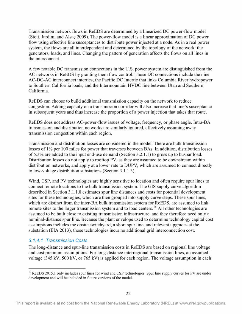
22


Transmission network flows in ReEDS are determined by a linearized DC power-flow model (Stott, Jardim, and Alsaç 2009). The power-flow model is a linear approximation of DC power flow using effective line susceptances to distribute power injected at a node. As in a real power system, the flows are all interdependent and determined by the topology of the network: the generators, loads, and lines. Changing the pattern of generation affects the flows on all lines in the interconnect.

A few notable DC transmission connections in the U.S. power system are distinguished from the AC networks in ReEDS by granting them flow control. Those DC connections include the nine AC-DC-AC interconnect interties, the Pacific DC Intertie that links Columbia River hydropower to Southern California loads, and the Intermountain HVDC line between Utah and Southern California.

ReEDS can choose to build additional transmission capacity on the network to reduce congestion. Adding capacity on a transmission corridor will also increase that line’s susceptance in subsequent years and thus increase the proportion of a power injection that takes that route.

ReEDS does not address AC-power-flow issues of voltage, frequency, or phase angle. Intra-BA transmission and distribution networks are similarly ignored, effectively assuming away transmission congestion within each region.

Transmission and distribution losses are considered in the model. There are bulk transmission losses of 1% per 100 miles for power that traverses between BAs. In addition, distribution losses of 5.3% are added to the input end-use demand (Section 3.2.1.1) to gross up to busbar load. Distribution losses do not apply to rooftop PV, as they are assumed to be downstream within distribution networks, and apply at a lower rate to DUPV, which are assumed to connect directly to low-voltage distribution substations (Section 3.1.1.3).

Wind, CSP, and PV technologies are highly sensitive to location and often require spur lines to connect remote locations to the bulk transmission system. The GIS supply curve algorithm described in Section 3.1.1.8 estimates spur line distances and costs for potential development sites for these technologies, which are then grouped into supply curve steps. These spur lines, which are distinct from the inter-BA bulk transmission system for ReEDS, are assumed to link remote sites to the larger transmission system and to load centers.16 All other technologies are assumed to be built close to existing transmission infrastructure, and they therefore need only a nominal-distance spur line. Because the plant envelope used to determine technology capital cost assumptions includes the onsite switchyard, a short spur line, and relevant upgrades at the substation (EIA 2013), those technologies incur no additional grid interconnection cost.

3.1.4.1 Transmission Costs The long-distance and spur-line transmission costs in ReEDS are based on regional line voltage and cost premium assumptions. For long-distance interregional transmission lines, an assumed voltage (345 kV, 500 kV, or 765 kV) is applied for each region. The voltage assumption in each

16 ReEDS 2015.1 only includes spur lines for wind and CSP technologies. Spur line supply curves for PV are under development and will be included in future versions of the model.

23


BA for long-distance transmission is taken from the highest voltage line currently operating in the BA from the Homeland Security Infrastructure Project (HSIP 2012). For BAs where the highest voltage of currently operating transmission lines is less than 500 kV, the voltage in the future is assumed to be 765 kV, and the associated costs for 765-kV lines are used for all years. For BAs where the highest voltage of currently operating transmission lines is 500 kV, the costs for 500-kV lines are used. The only exception to these rules for voltages in the Eastern Interconnection are for BAs in New England (Connecticut, Maine, Massachusetts, New Hampshire, Rhode Island, and Vermont), which are assumed to use 345-kV transmission lines for all years.

Each voltage class is associated with a base capital cost sourced from the Phase II Eastern Interconnection Planning Collaborative (EIPC) report: $2,333/MW-mile, $1,347/MW-mile, and $1,400/MW-mile for 345-kV, 500-kV, and 765-kV transmission lines, respectively (EIPC 2012).17 All wind and solar spur line costs are based on 230-kV line costs, assumed to be $3,667/MW-mile (ibid).18

In addition to the base transmission costs, regional multipliers are also applied and are largely based on assumptions from the EIPC report. Regional transmission cost multipliers are the average of the EIPC report’s high and low multipliers in each North American Electricity and Environmental Model (NEEM) region and are associated with the assumed voltage within the region. BAs in ERCOT and the Western Interconnection (excluding Canada and California) are assumed to have a regional transmission multiplier of one (1). Long-distance transmission costs in BAs in the California Independent System Operator (CAISO) are 2.25 times the cost of the other baseline costs for the rest of the Western Interconnection. For long-distance transmission between BAs with different transmission costs, the average cost is used. The same process is applied for wind and solar spur line costs.

Figure 13 and Figure 14 show the regional long-distance and spur-line transmission costs, respectively, resulting from the previously described steps and assumptions.

17 The base transmission costs for ReEDS are converted to $/MW-mile according to new transmission line cost and capacity assumptions for single circuit conductors for each voltage in the EIPC (2012) report. The costs reported are in 2010$ as used by the EIPC. 18 Wind and solar spur line costs are applied within the development of the resource supply curves (see Section 3.1.1.8).

24


Figure 13. Map of long-distance transmission costs

Figure 14. Map of spur-line transmission costs

25


3.2 Electricity System Operation and Reliability ReEDS finds the least-cost way of building and operating the electricity system while meeting certain requirements. Those requirements are dominated by the need to meet electricity load while maintaining system adequacy and operational reliability.

3.2.1 Electricity Load The primary constraint in ReEDS is to serve electricity load in each BA and time-slice. The end-use electricity demand projection used in ReEDS is exogenously defined, based on scenarios from AEO 2014 and calibrated in 2010 to load data from Ventyx (2014) and EIA (2014a). Specifically, hourly load profiles from Ventyx transmission zones are summarized and averaged to the 17 time-slice load profiles for the model BAs. These 2010 profiles are then scaled to ensure a match with the state-level annual load data from EIA’s “Electricity Data Browser” (EIA 2012). The load growth factors for years after 2010 are calculated from the AEO 2014 Reference scenario load projections by census regions (EIA 2014a).19 For each solve year in ReEDS, the regional load profiles are increased by regional growth factors.20

The end-use demand, described in the previous paragraph, is defined at the meter level. ReEDS includes transmission system losses in its algorithms, but not distribution losses, so the load target for ReEDS is busbar load, requiring end-use demand to be grossed up to account for distribution losses. The 5.3% distribution loss factor is estimated based on a combination of EIA and ReEDS figures. ReEDS is required to generate sufficient power in each time-slice and BA (allowing for transmission of power, but accounting for losses) to meet this busbar demand.

3.2.1.1 System Adequacy Planning reserve requirements ensure that adequate generating capacity is available at all times. In practice, this is enforced by requiring the system to have sufficient firm capacity to meet the forecasted peak demand plus a reserve margin. Each technology is assigned a capacity credit reflecting its expected availability when power is needed. For conventional generators, the capacity value matches the nameplate capacity. For variable resource renewable energy technologies (i.e., wind and solar), ReEDS estimates a fractional capacity value for each region/class bin via a statistical effective load carrying capability (ELCC) calculation performed between solves.

The ELCC calculation is based on the relationship between VRRE output and load, accounting for existing contributions from other VRRE sources and the correlations among those sources, and it can be described as the amount of additional load that can handled with those generators in place compared to without them, while maintaining a constant loss-of-load probability. Before

19 The demand growth factors from AEO’s census regions are applied to the ReEDS NERC-level regions. Due to differences in AEO’s census regions and the similarly sized NERC regions in ReEDS, the projected national load in ReEDS does not agree exactly with AEO’s demand projections, but the differences are small. 20 For years after 2040 for which AEO does not have projections, the average growth rate projected between 2030 and 2040 is used. Demand profiles and annual consumption can be altered with different plug-in hybrid electric vehicle and rooftop PV scenarios; however, absent these demand-side technologies, the profiles are assumed to be the same as those from 2010.

26


each solve year, ReEDS calculates both the ELCC of all existing VRRE capacity and a hypothetical ELCC for any candidate VRRE capacity that might be built in the coming year.

The reserve margin fractions applied in ReEDS are based on reserve margin requirements for NERC reliability regions (North American Electric Reliability Corporation (NERC) 2010). Each BA must meet the requirement, but BAs are allowed to engage in bilateral contracts for firm capacity as long as space remains on transmission lines after accounting for power flows.

3.2.1.2 Operational Adequacy In addition to ensuring adequate capacity to satisfy long-term planning reserve requirements, ReEDS requires adequate operating reserve capacity to meet daily operating reserve requirements. Operating reserve requirements ensure that there is sufficient flexibility from supply-side and demand-side technologies to rebalance fluctuations in generation and demand. For ancillary services below the 4-hour to 8-hour resolution of ReEDS time-slices, ReEDS assumes statistically computed operating reserve requirements for load and variable supply and requires that capacity with adequate flexibility is available to handle such events. All operating reserves requirements must be satisfied in each BA in each time-slice; however, reserve provision can be shared between BAs in the same manner as firm capacity is traded.

The flexibility of generators and storage technologies depend on the ability of the plant to change its output and the time scales necessary to do so. Given start-up times and ramp rates, technologies are classified to be able to offer varying amounts of spinning or quick-start reserves. Spinning reserves can be provided by generation and storage technologies that are on but not fully dispatched in a given time-slice. The amount of capacity that may be counted toward the requirements depends on the amount that can be ramped up quickly (e.g., within 10 minutes). Technologies that can start generating power quickly from a cold state (again, within 10 minutes; e.g., natural gas combustion turbines), have the option of offering quick-start reserves. In addition, demand-side interruptible load can also contribute to reserve requirements, if enabled in a scenario.

The operating reserve requirements in ReEDS represent multiple ancillary services covering contingency, frequency regulation, and VRRE forecast error reserves.

• Contingency reserve requirements: These requirements ensure that an unanticipated change to the operational status of generators or transmission lines (e.g., changes due to unforeseen outages) will not cause an extended disruption to electricity end users. In ReEDS, the contingency reserve requirement is set at 6% of demand in each time-slice (Zavadil et al. 2004). At least half of this requirement must be met with spinning reserves or interruptible load, while the other half can be met by quick-start units. The relevant time scale for contingency events is about 10 minutes.

• Frequency regulation reserve requirements: These requirements ensure that sub- minute deviations between demand and generation can be minimized. Due to the short time scales involved, only spinning reserves can satisfy the frequency regulation requirements. In ReEDS, this requirement is set at 1.5% of average demand in each time- slice (Zavadil et al. 2004).

• VRRE forecast error reserve requirements: These requirements ensure stability of the system despite uncertainties in forecasting for wind and PV.

Generally, forecast error

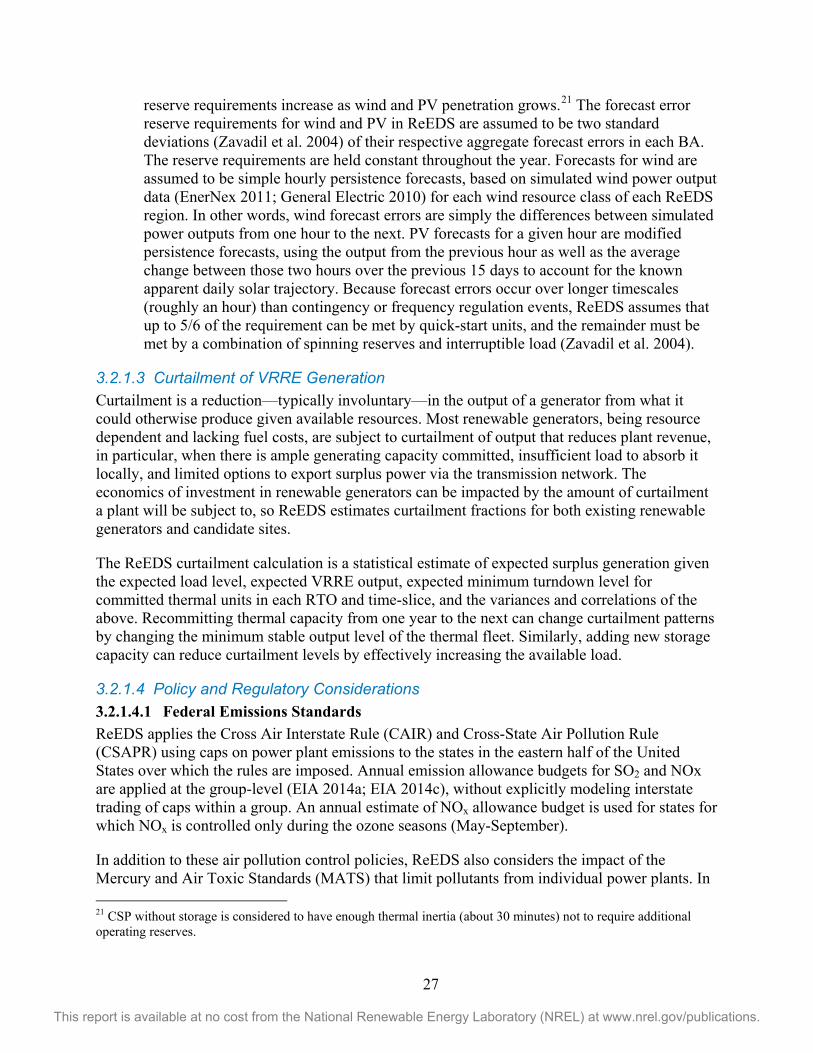
27


reserve requirements increase as wind and PV penetration grows.21 The forecast error reserve requirements for wind and PV in ReEDS are assumed to be two standard deviations (Zavadil et al. 2004) of their respective aggregate forecast errors in each BA. The reserve requirements are held constant throughout the year. Forecasts for wind are assumed to be simple hourly persistence forecasts, based on simulated wind power output data (EnerNex 2011; General Electric 2010) for each wind resource class of each ReEDS region. In other words, wind forecast errors are simply the differences between simulated power outputs from one hour to the next. PV forecasts for a given hour are modified persistence forecasts, using the output from the previous hour as well as the average change between those two hours over the previous 15 days to account for the known apparent daily solar trajectory. Because forecast errors occur over longer timescales (roughly an hour) than contingency or frequency regulation events, ReEDS assumes that up to 5/6 of the requirement can be met by quick-start units, and the remainder must be met by a combination of spinning reserves and interruptible load (Zavadil et al. 2004).

3.2.1.3 Curtailment of VRRE Generation Curtailment is a reduction—typically involuntary—in the output of a generator from what it could otherwise produce given available resources. Most renewable generators, being resource dependent and lacking fuel costs, are subject to curtailment of output that reduces plant revenue, in particular, when there is ample generating capacity committed, insufficient load to absorb it locally, and limited options to export surplus power via the transmission network. The economics of investment in renewable generators can be impacted by the amount of curtailment a plant will be subject to, so ReEDS estimates curtailment fractions for both existing renewable generators and candidate sites.

The ReEDS curtailment calculation is a statistical estimate of expected surplus generation given the expected load level, expected VRRE output, expected minimum turndown level for committed thermal units in each RTO and time-slice, and the variances and correlations of the above. Recommitting thermal capacity from one year to the next can change curtailment patterns by changing the minimum stable output level of the thermal fleet. Similarly, adding new storage capacity can reduce curtailment levels by effectively increasing the available load.

3.2.1.4 Policy and Regulatory Considerations 3.2.1.4.1 Federal Emissions Standards ReEDS applies the Cross Air Interstate Rule (CAIR) and Cross-State Air Pollution Rule (CSAPR) using caps on power plant emissions to the states in the eastern half of the United States over which the rules are imposed. Annual emission allowance budgets for SO2 and NOx are applied at the group-level (EIA 2014a; EIA 2014c), without explicitly modeling interstate trading of caps within a group. An annual estimate of NOx allowance budget is used for states for which NOx is controlled only during the ozone seasons (May-September).

In addition to these air pollution control policies, ReEDS also considers the impact of the Mercury and Air Toxic Standards (MATS) that limit pollutants from individual power plants. In 21 CSP without storage is considered to have enough thermal inertia (about 30 minutes) not to require additional operating reserves.

28


contrast to the CAIR and CSAPR implementations, MATS is applied by requiring the coal fleet to retrofit into compliance in 2016. In general, plants that are expected to retire within a few years after 2016 are assumed to install fabric filters and dry sorbent injection (DSI), while longer-lasting units pay for more-complete flue-gas desulfurization (FGD) upgrades for units that do not already have SO2 scrubbers. Rather than being treated as decisions within the model, these upgrades are mandated in ReEDS, with retrofit costs applied to the system cost and the calculated electricity price. The expected capacity-weighted average cost of retrofit options for MATS compliance is used as a proxy for representing an estimate of overall MATS retrofit cost22 in ReEDS.

While MATS is primarily designed to limit the mercury (Hg), hydrochloride (HCl) and particulate matter (PM), there are also alternate limits in terms of other metallic/non-metallic pollutants, including SO2. Therefore, ReEDS models the consequence of MATS compliance in terms of SO2 emission factor change for the major technologies that are expected to undergo retrofits. While ReEDS does not control mercury emissions, it does track them beyond the planning horizon and the MATS compliance effects are incorporated by reducing Hg emission factors for these generation technologies by 90% during post-MATS period.

California’s Assembly Bill 32 (AB-32) is modeled as a cap on electricity-system CO2 emissions from generators in California itself or serving load in California. Direct CO2 emissions from generators located in California count toward the cap. Imported carbon is estimated through an accounting of imported energy and carbon intensity of the BAs from which that energy originated. The similar Regional Greenhouse Gas Initiative (RGGI) regulation in New England is not implemented in ReEDS at this time. Proposed or draft EPA regulations, including the Clean Power Plan, are not modeled in the current version of ReEDS.

3.2.1.4.2 State Renewable Standards Table 12 presents the renewable portfolio standard (RPS) goals used in Central Scenario as obtained from the Database of State Incentives for Renewables & Efficiency (DSIRE) (EPA 2014). The state RPS requires a utility to install or generate a certain fixed amount of renewable capacity or energy. The effective RPS requirements in Table 12 account for how RPS rules commonly apply different fractions to different load-serving entities within a state (e.g., California’s RPS is modeled as 31.7% in 2020 instead of 33%). States also have unique rules about eligible renewable technologies and eligible imports, which ReEDS represents through a system of trading renewable energy certificates (RECs). Delaware, Illinois, Massachusetts, Maryland, Minnesota, Missouri, New Hampshire, New Jersey, New Mexico, Nevada, Ohio, and Pennsylvania have chosen to encourage the widespread use of solar technologies by stipulating a solar set-aside, which requires that a certain fraction of the RPS be met specifically with solar resources.

22 The capacity of retrofits estimated by EPA’s regulatory impact analysis, in combination with costs from the NEMS Electricity Market Module, is used to calculate a common capacity-weighted retrofit cost in $/kW (e.g., about $84.3/kW in 2013$ for the average non-FGD option).

29


Table 12. Effective State RPS requirements in ReEDS Start Year Full

Implementation RPS (%)

AZ 2006 2025 6.2

CA 2004 2020 31.7

CO 2007 2020 21.2

CT 2006 2020 21.5

DE 2008 2027 17.5

IL 2008 2026 22.2

KS 2011 2020 16.3

MA 2004 2050 41.4

MD 2006 2022 18.7

ME 2000 2017 39.3

MI 2012 2015 10.0

MN 2010 2025 28.3

MO 2011 2021 10.2

MT 2008 2015 10.0

NC 2010 2021 11.9

NH 2008 2025 23.4

NJ 2005 2021 17.6

NM 2006 2020 15.6

NV 2005 2025 22.1

NY 2003 2015 24.4

OH 2009 2024 11.1

OR 2011 2025 20.4

PA 2007 2021 17.5

RI 2007 2019 15.9

WA 2012 2020 12.7

WI 2006 2015 9.6

30


3.2.1.4.3 State and National Tax Incentives Existing federal tax incentives for renewable energy are included in the Central Scenario. Specifically, the wind production tax credit (PTC) and investment tax credit (ITC) are assumed to expire after the 2014 solve year.23 The Modified Accelerated Cost Recovery System (MACRS) depreciation schedules remain in place for all years, as it is a permanent part of the tax code. The solar ITC is assumed to be 30% through 2016, after which it is assumed to remain at 10% through 2050. The geothermal ITC is assumed to be 10% for all years.

Several states also have production and investment incentives for renewable energy sources. The values used in the Central Scenario are listed in Table 13. While states in addition to North Dakota have ITCs on the books, those programs are for small system installations and have dollar amount limits that render them of limited value for ReEDS’ utility-scale investments.

Table 13. State Tax Incentives included in the Central Scenario State PTC ($/MWh) ITC (%)

Maryland 8.5 -

North Dakota - 15

New Mexico 10.0 -

Oklahoma 5.0 -

Utah 3.5 -

3.3 Capital Financing, System Cost, and Electricity Rates 3.3.1 Financing of Capital Stock ReEDS uses generalized financial assumptions that are standardized across technologies in order to compare different technologies and projects. Using a standardized method allows for consistently comparing technologies without projecting technology-specific risk profiles or specialized financing vehicles into the future. In other words, these simplified assumptions allow different projects and technologies to be compared and to compete across the long time horizon and spatial extent of ReEDS.

Using a utility-owned project perspective, ReEDS discounts future transactions, accounts for tax benefits, and weighs risk where possible. Table 14 lists the major financing parameters used in the ReEDS analysis. All costs, including new capital investments, O&M costs, fuel costs, and transmission investments, are considered on a 20-year net present value basis. The discount rate used in the present value evaluation is the weighted average cost of capital based on the parameters shown by Table 14 and is 8.9% nominal (6.2% real).24

23 The 2014 solve year represents 2013 and 2014. The PTC that expired at the end of 2013 includes provisions that allow new projects to qualify for the tax credit even if they do not begin operating after it expires. ReEDS includes prescribed new wind capacity in the near term to account for post-2013 effect of the PTC on new wind deployment. 24 ReEDS considers all costs in real dollar terms, but the parameters presented in Table 14 are primarily nominal.

31


Table 14. Key Financial Assumptions Evaluation Period 20 years

Inflation Rate 2.5%

Interest Rate – Nominal 8%

Rate of Return on Equity – Nominal 13%

Debt Fraction 50%

Combined State and Federal Tax 40%

Weighted Avg. Cost of Capital – Nominal (Real) 8.9% (6.2%)

Modified Accelerated Cost Recovery System (MACRS) (non-hydropower renewables) 5 years

MACRS (nuclear, combustion turbines) 15 years

MACRS (other fossil, hydropower, storage) 20 years

Key parameters for the weighted average cost of capital include the assumed rate of return on equity (RROE), the allowed debt fraction, and the debt interest rate. The nominal 13% RROE assumption is intended to reflect long-term RROEs for a broad range of corporations and electric generation projects, and generally, it falls within the ranges of RROEs reported elsewhere. For example, according to Edison Electric Institute (EEI), approved RROEs since 1990 for regulated investor-owned utilities have ranged from 10.0% to 12.9%, with an average awarded RROE of 11.2% (EEI 2010b). The California Energy Commission (CEC), meanwhile, assumed an average rate of return on equity capital of 11.9% for investor-owned utility generation and 14.5% for merchant-based generation (CEC 2009). The National Energy Technology Laboratory (NETL) recommended a slightly higher RROE of 20% for Independent Power Producer (IPP) development of fossil-based resources (NETL 2008).

The debt fraction of 50% is an amalgam of recent utility and IPP practices. According to the Edison Electric Institute, as of end-of-year 2008, investor owned utilities had an aggregate debt fraction of 59%, up from 56% in 2007 and 2006 (EEI 2009). The California Energy Commission assumed an average investor-owned utility (IOU) debt fraction of 48% for investor owned utility generation and 40%–60% for merchant based generation (CEC 2009). Additionally, NETL recommend debt ratios of 45%–70% for IOU and IPP developed generation assets (NETL 2008).

The debt interest rate assumption of 8% used in this study is roughly consistent with a long-term corporate bond interest rate forecast in EIA’s AEO 2010. EIA forecasted a 7.6% average interest rate for AA rated utility bonds through the year 2035 (EIA 2010). The AA-rated utility bond would generally represent the borrowing cost for a project developed by an investment grade IOU. The debt interest rate during construction is assumed to be consistent with the term debt (Harper, Karcher, and Bolinger 2007).

In addition to the general financial assumptions, some technology-specific parameters are used within ReEDS. In particular, technology-specific construction periods yield different construction financing costs. Tax credits and accelerated tax depreciation rules also yield different financing effects across technologies.

32


3.3.2 Calculating Total System Cost Two system-wide cost metrics are calculated from each ReEDS run: a present value of direct electric sector system costs and a retail electricity price. These cost calculations are not part of the ReEDS optimization process but are calculated after the ReEDS optimizations have been conducted. The direct electric sector costs represent the present value cost of building and operating the system over the scenario horizon. The methodology to calculate electricity prices is described in next section.

The system cost metric is intended to encompass capital and operating costs for ReEDS electricity system infrastructure, in present value terms. The costs in future years are discounted by a social discount rate.25 To reflect that substantial value remains in the capital stock when the scenario halts in 2050, capital investments within 20 years of the model horizon are prorated based on how much book lifetime remains after 2050.

Cost components included in the system cost metric are fully loaded capital costs for generating capacity and transmission lines, fixed and variable O&M costs, and fuel expenditures. Capital and operating costs are accounted differently in the calculation; capital investments are charged the all-in capital cost in the year the plant comes online (minus salvage value), while operating costs accrue over the operating life of the plant. Notably, because a ReEDS solve touches only even-numbered years, the operating costs are all doubled; for example, fuel expenditures for 2016 alone doubled approximate fuel expenditures in 2015 and 2016.

3.3.3 Estimating Retail Electricity Rates The ReEDS electricity price estimate is reported as a retail electricity rate for each BA and year. The retail electricity price comprises 1) cost recovery for capital stock, through a 30-year rate-base structure; 2) operating expenditures, directly; and 3) an estimated wholesale-to-retail markup for “non-generation transaction costs.”

The electricity price calculation assumes a regulated market structure with a 30-year rate-base, or amortization of all investments to 30 equal annual payments. Each year, eligible investments—i.e., new and replacement generating capacity and new transmission lines—are added to the rate-base. Also each year one thirtieth of the standing rate-base, plus interest, is slotted for repayment, and so recovered via electricity rates. Operating costs, in contrast, are recovered immediately each year.

A cost of generation in each BA is calculated as the sum of the rate-base repayment and the operating expenses, divided by electricity generated. Because not all electricity is consumed locally, the wholesale cost of electricity at each BA is calculated based on the cost of generation from all sources serving the region and their relative contributions.

In addition to the wholesale cost of power, the retail price of electricity must cover distribution costs as well as general administrative costs for the utility (e.g., billing, facilities, and management). These additional costs are not estimated directly in ReEDS. Instead the markup

25 The discount rate (3% real) used for the present value system cost represents the social discount rate, and it is not the same as the discount rate used in the investment decisions within the optimization.

33


from wholesale to retail electricity price is based on the difference between the wholesale electricity price calculated in ReEDS after the 2010 solve and reported retail prices for 2010 (Ventyx 2014), redistributed from service territories to ReEDS BAs based on population. The difference between this model-calculated wholesale price and the historical retail price is used to markup the wholesale electricity price in all subsequent years.

34


4 Central Scenario Results The Central Scenario described here is the scenario executed with the base settings described above. This report also includes an ensemble of scenarios with alternative parameter settings or with other model options or capabilities switched on (see Section 5). The Central Scenario is the result of ReEDS v.2015.1 with default settings, and it is therefore a useful benchmark for understanding the baseline behavior of this model version.

Despite steady load growth and continuation of existing policies, the Central Scenario presides over a dramatic transition in electricity provision in the United States (see Figure 15 and Figure 16). Load in the scenario grows through 2050, requiring slow growth in generating stock to meet the increases. Meanwhile, as the aging electricity fleet the model begins with in 2010 retires—a third of the capacity that existed in 2010 retires before 2040, and almost half by the end of the model horizon in 2050—shifting economics guarantee that retiring stock is replaced by a different portfolio of technologies.

Figure 15. Cumulative installed capacity by technology type in the Central Scenario

0

200

400

600

800

1000

1200

1400

1600

1800

2010

2012

2014

2016

2018

2020

2022

2024

2026

2028

2030

2032

2034

2036

2038

2040

2042

2044

2046

2048

2050

Cap

acity

(GW

)

StorageSolarWindBiopowerGeothermalHydroGas-CTGas-CCOil-Gas-SteamCoalNuclear

35


Figure 16. Generation by technology in each solve year in the Central Scenario

One clear dynamic is a shift from coal to natural gas, continuing the trend of the past decade (Figure 17). Persistently low natural gas prices keep natural gas combined cycle plants competitive, and thus increasing their market share, as the coal fleet is steadily phased out. After two decades of slow transition, increasing coal retirements in the 2040s sets the stage for natural gas generation to exceed coal for the first time in the middle of that decade.

Figure 17. Transition from coal to natural gas, past, present, and future

Figure 18. Growth in wind and solar generation, past, present, and future

0

1000

2000

3000

4000

5000

6000

2010

2012

2014

2016

2018

2020

2022

2024

2026

2028

2030

2032

2034

2036

2038

2040

2042

2044

2046

2048

2050

Gen

erat

ion

(TW

h)

Imports

Solar

Wind

Biopower

Geothermal

Hydro

Gas-CT

Gas-CC

Oil-Gas-Steam

Coal

Nuclear

0

0.2

0.4

0.6

0.8

2000 2010 2020 2030 2040 2050

Frac

tion

of G

ener

ated

El

ectr

icit

y

Historical Coal ReEDS Coal

Historical NG ReEDS NG

0.0001

0.001

0.01

0.1

1

2000 2010 2020 2030 2040 2050

Frac

tion

of G

ener

ated

El

ectr

icit

y

Historical Wind ReEDS Wind

Historical Solar ReEDS Solar

36


The Central Scenario also sees substantial growth in investment in and generation from renewable generation technologies, especially land-based wind power and photovoltaics (see Figure 18). Installed wind capacity grows from 65 gigawatts (GW) in 2014 to nearly 300 GW in 2050, and solar expands to almost 400 GW. These trends again continue dramatic recent historic growth, bringing the power sector from a minor (<1%) contribution from wind and solar in 2000, through nearly 6% of generation today, and on to 36% of generation in 2050.

As these shifts in generation source take effect, the impacts on operation play out in a more flexible power system. In ReEDS’ 2010 operation, coal and nuclear plants provide a steady supply of power year-round (70% of total production) while hydropower and natural gas follow load and provide ancillary services. However, by 2050 traditional baseload generators provide only a fifth of total generation (see Figure 19 and Figure 20). Instead, the gas-CC fleet provides bulk power that is responsive to electricity consumption profiles and renewable generator production—providing more power when needed, and less when the sun shines and wind blows. The residual load, load minus variable renewable output (e.g., wind and PV), has been reshaped; evenings and even some overnight time-slices, when the solar-powered capacity is unavailable, become the periods with greater average need for fossil power.

Figure 19. Generation by time-slice in 2010 in the Central Scenario

0

100

200

300

400

500

600

700

800

Ave

rage

Gen

erat

ion

(GW

)

Time Slice

Imports

Solar

Wind

Geothermal

Hydro

Biopower

Oil-Gas-Steam

Gas-CT

Gas-CC

Coal

Nuclear

37


Figure 20. Generation by time-slice in 2050 in the Central Scenario

Carbon intensity of electricity generation in the United States has declined from mid-20th century levels, but it stayed roughly flat through the 1990s and most of the 2000s (EIA 2014c), before trending downward with the coal-to-gas shift that occurred with the growth of unconventional gas drilling. In the Central Scenario, a downward trend continues into the future (Figure 21), first with the continuation of the transition from coal to gas, assisted by adoption of low-carbon renewable power, then accelerated by coal fleet retirements in the 2040s.

Figure 21. Carbon intensity of the electricity system (direct emissions)

Current regulation and policy, combined with present projections for technology and fuel costs, produce over four decades a United States power system distinctly different from the traditional base-intermediate-peak dynamic, and fossil-fuel dominated power system of even the recent past. This scenario, of course, represents only one of many possible visions of the future. In the following sections of this report, we outline and explore an ensemble of alternative scenarios, with different technology projections, fuel costs, policy environments, and more.

0

100

200

300

400

500

600

700

800

900

1000

Ave

rage

Gen

erat

ion

(GW

)

Time Slice

Imports

Solar

Wind

Geothermal

Hydro

Biopower

Gas-CT

Gas-CC

Coal

Nuclear

0

0.2

0.4

0.6

0.8

1

1950 1970 1990 2010 2030 2050

Car

bon

Inte

nsity

(kg

CO

2/kW

h)

HistoricalReEDS

38


5 Standard Scenarios Ensemble Some of the scenarios in this ensemble involve changes in parameters generally considered influential on the evolution of the power sector: fuel prices, rate of demand growth, technological improvement, and the retirement schedule of today’s fleet. For these scenarios, we include two scenarios in the ensemble that vary in both directions from the baseline assumption in the Central Scenario. Other scenarios are more individually defined, each as its own vision of the future, distinct from the Central Scenario. These other scenarios demonstrate a few ReEDS model options or capabilities to provide context for how these options can change the model’s behavior. Table 15 summarizes the Standard Scenarios.

Table 15. Summary of the Standard Scenarios. The scenario settings listed in blue italics correspond to the setting in the Central Scenario.


Fossil Fuel Prices

Reference Fuel Prices AEO 2014 Natural Gas (NG) and Coal Reference

Low Fuel Prices AEO 2014 High Oil & Gas Resource, Low Coal Price

High Fuel Prices AEO 2014 Low Oil & Gas Resource, High Coal Price

Electricity Demand Growth

Reference Demand Growth AEO 2014 Reference

Low Demand Growth AEO 2014 Low Economic Growth

High Demand Growth AEO 2014 High Economic Growth

Vehicle Electrification PEV/PHEV adoption reaches 30% of sales by 2050; 45% of charging utility-controlled, 55% opportunistic

Renewable Energy Technology Costs

Mid RE Cost Annual Technology Baseline (ATB) Mid-Case Projections

Low RE Cost Annual Technology Baseline (ATB) Low-Case Projections

High RE Cost Annual Technology Baseline (ATB) High-Case Projections

RE Technology Improvement EERE program office technology cost and performance goals

Existing Fleet Retirements Reference Retirement

Generator Database and Online Year (Ventyx); Planned Coal Retirements (M.J. Bradley)

39



Extended Nuclear Lifetime Relicensing to 80 years

Accelerated Coal Retirement 50-year lifetime if built after 1970 (from 65+); Accelerated retirement if built before 1970

Policy/Regulatory Environment

Extended Incentives for RE Generation Extend ITC/PTC through 2030 for eligible technologies

National Renewable Portfolio Standard (RPS)

43% of generated electricity from renewables by 2030, 80% by 2050

Power Sector CO2 Cap President’s Climate Goal: power sector emissions 17% below 2005 levels by 2020, 83% by 2050

Current Law Used for the Central Scenario

Earth System Feedbacks Impacts of Climate Change

Temperature impacts on generators, transmission, and load; derived from IGSM-CAM climate scenario

Resource and System Constraints

Reduced RE Resource Simple 25% cut to resource in input supply curves

Barriers to Transmission System Expansion

3x transmission capital cost No new AC-DC-AC interties 2x transmission loss factors

Restricted Cooling Water Use New construction may not use freshwater for cooling

Generation Technology Improvement

Nuclear Technology Breakthrough 40% reduction in nuclear capital costs

To enable better visualization and interpretation of the model outputs, results will be presented in two groups. Scenarios with bidirectional parameter changes—fuel prices, rate of demand growth, technological improvement, and fleet retirements—are presented in Sections 5.1 through 5.4, and the outputs of those scenarios are discussed together in Section 5.5. The remaining scenarios are discussed in Sections 5.6 through 5.15. The Appendix includes the same plots as Section 5.5 but for the scenarios that are not discussed in Section 5.5.

40


5.1 Fossil Fuel Prices For these scenarios, we use two alternative natural gas scenarios to the AEO 2014 Reference scenario, based on the Low Oil and Gas Resource and High Oil and Gas Resource scenarios from AEO 2104 (EIA 2014a). The analysis also relies on two alternative coal price trajectories from AEO 2014: High Coal Price and Low Coal Price. As with the Central Scenario assumptions, the coal price is assumed fully inelastic, while the natural gas prices are dynamic through the supply curve structure discussed in Section 3.1.2.3. In Figure 22, therefore, the coal price shown is exactly the price seen in ReEDS, while the path displayed for natural gas is the AEO scenario price (and flat from 2040 to 2050), and the output ReEDS price is dependent on demand. All scenarios rely on the same uranium price projection shown in Section 3.1.2.3.

Figure 22. Alternate natural gas and coal price scenarios

5.2 Demand Growth Long-term electricity load projections are highly uncertain, as can be seen by reviewing load growth projections from 10 and 20 years ago. Nevertheless, a deterministic scenario must have a single projection for future load; thus, to explore how the electric sector evolves differently in other load-growth regimes, these two scenarios bracket the central load projection based on different macroeconomic growth rates. The Central Scenario is based on the AEO 2014 Reference scenario load; the high and low load growth scenarios are also from AEO 2014: the “High Economic Growth” and “Low Economic Growth” scenarios, which use higher/lower rates of population growth, productivity, and lower/higher inflation than the Reference (see Figure 23). The AEO “High” has 2.8% annual GDP growth compared to 2.4% in the “Reference” and 1.9% in the “Low” case (EIA 2014a, 20). For years after the NEMS model horizon in 2040, we assume an annual growth rate equal to the average growth rate from 2030 to 2040. From 2020 to 2050, the High Economic Growth Scenario grows at an average annual rate of about 1.1% per year, compared to the Central Scenario growing at about 0.7% per year and the Low Economic Growth Scenario growing at less than 0.4% per year. For comparison, average annual growth rate from 1990 to 2013 was 1.3% per year (EIA 2014a).

$0

$2

$4

$6

$8

$10

$12

2010 2020 2030 2040 2050

NG

Fue

l Pri

ce (2

013$

/MM

Btu

)

$0

$2

$4

$6

$8

$10

$12

2010 2020 2030 2040 2050

Coa

l Fue

l Pri

ce (2

013$

/MM

Btu

) High Fuel PricesReference Fuel PricesLow Fuel Prices

41


Figure 23. Alternate load pathways

5.3 Renewable Energy Technology Costs These scenarios use alternative cost and performance trajectories for land-based and offshore wind, solar PV, and CSP technologies. A summary of these alternative trajectories is presented here. Details can be found in the ATB spreadsheet and PowerPoint presentation that accompany this report (NREL 2015). Figure 24 and Figure 25 contain input cost assumptions for TRG 2 land-based and offshore wind, respectively. Similar trajectories exist for each TRG. Figure 26 shows the variation of photovoltaic future trajectories. Cost trajectories for CSP with six hours of storage are shown in Figure 27. Cost and performance trajectories for all variations of these technologies are presented in the ATB spreadsheet.

Figure 24. High, medium, and low overnight capital cost trajectories for TRG 2 land-based wind generators.

The mid case is used in the Central Scenario.

0

1000

2000

3000

4000

5000

6000

2010 2020 2030 2040 2050

End

-Use

Ele

ctri

city

Dem

and

at B

us

Bar

(TW

h)

High Econ GrowthReferenceLow Econ Growth

0

200

400

600

800

1000

1200

1400

1600

1800

2010 2020 2030 2040 2050

TR

G 2

Lan

d-B

ased

Win

d C

apita

l Cos

ts (2

013$

/kW

)

HighMidLow

42


Figure 25. High, medium, and low overnight capital cost trajectories for TRG 2 offshore wind generators.

The mid case is used in the Central Scenario.

Figure 26. High, medium, and low overnight capital costs for UPV. The mid case is used in the Central Scenario.

0

1000

2000

3000

4000

5000

6000

2010 2020 2030 2040 2050

TR

G 2

Off

shor

e W

ind

Cap

ital

Cos

ts (2

013$

/kW

) High

Mid

Low

0500

100015002000250030003500400045005000

2010 2020 2030 2040 2050

UPV

Cap

ital

Cos

ts (2

013$

/kW

)

HighMidLow

43


Figure 27. High, medium, and low overnight capital costs for CSP with 6 hours of TES. The mid case is used in the Central Scenario.

5.4 Existing Fleet Retirements The Central Scenario age-based retirement assumptions described in Section 3.1.2.4 result in nearly all of the existing (2012) oil/gas steam turbines and existing nuclear units being retired by 2050.26 By 2050, about half of the existing coal capacity is also retired, based solely on the age-based retirement assumptions. Age-based retirements have a lesser impact on natural gas capacity, with only about 35% of today’s NG-CT capacity and about 10% of the NG-CC capacity retired by 2050.

In a given load-growth scenario, the retirement pathway of the existing fleet is a strong determinant of how much new capacity must be built to serve load and maintain reliability. In general, the higher the retirement rate, the more new capital stock is required. With this in mind, we include two scenarios to bracket the Central Scenario with alternative retirement futures: one with accelerated coal retirements and one in which most of today’s nuclear fleet successfully completes a second relicensing to attain an ultimate 80-year operational life. The nationwide retirement pathways are shown in Figure 28. To be sure, these scenarios omit many equally valid possibilities for how today’s fleet matures—in particular, the technological asymmetry of these two scenarios carries specific regional determinism—but in general, the Accelerated Coal Retirement Scenario creates an opportunity for new generation to be built while maintaining the Central Scenario’s coal retirement schedule and extending the lifetime of the nuclear fleet means that a larger proportion of the eventual 2050 stock is legacy from 2014.

26 The age-based retirements result in essentially no nuclear retirements by 2030. However, recent and announced nuclear retirements (e.g., the San Onofre Nuclear Generating Station retirement in 2013) are included in ReEDS.

0100020003000400050006000700080009000

2010 2020 2030 2040 2050

Capi

tal C

ost f

or C

SP w

ith

6 hr

of

TES

(201

3$/k

W)

LowMidHigh

44


5.5 Range of Outcomes among the Bidirectional Scenarios Scenario outputs are grouped below by output type (e.g., wind generation, CO2 emissions), and they are shown for the subset of the scenarios described above on the same plot. This way of presenting results allows one to see the sensitivity of various input assumptions on the model outputs, as well as the range of outputs that can easily be spanned by the input ranges. Only a small subset of model outputs is shown below. Some major outputs, such as coal and nuclear generation, are not shown because the majority of the scenarios have similar profiles for those outputs.

5.5.1 Wind Generation Figure 29 shows the range of wind generation outputs for this subset of scenarios. Wind generation deviates most strongly from the Central Scenario under low and high fuel costs, and with low wind and solar costs. Scenarios that have greater capacity needs (High Economic Growth and Accelerated Coal Retirements) increase wind deployment as wind meets those needs, while the opposite is true for the scenarios that require less capacity (Low Economic Growth and Extended Nuclear Lifetime). In all of the scenarios in the figure, wind generation increases through 2050, though the rate and timing of these increases depend critically on the assumptions used.

0

20

40

60

80

100

120

2010 2030 2050 2070

Rem

aini

ng C

apac

ity

(GW

) Nuclear

ExtendedBaseline

050

100150200250300350

2010 2030 2050 2070

Rem

aini

ng C

apac

ity

(GW

)

Coal

BaselineAccelerated

Figure 28. Nuclear and Coal Retirement Pathways

45


Figure 29. Annual wind generation in the bidirectional scenarios. This range of generation corresponds to 145–379 GW of wind capacity in 2050.

5.5.2 Solar Generation Solar generation in the bidirectional scenarios is shown in Figure 30. The scenarios span a wide range of outputs, with the highest deployment producing five times more solar power than the lowest deployment. Many results follow the same trends as those seen in the wind generation discussed above, but there are several notable differences. The Low Cost Solar & Wind Scenario increases early solar deployment but reduces long-term solar deployment. This is because the solar cost inputs for the scenario only accelerate the cost decline to the SunShot 75% level (see Section 3.1.1.3) but do not lower cost below that level. The Central Scenario still reaches the SunShot 75% level, but in 2030 instead of 2020. From 2030 and on, the solar costs are the same in the Low Cost Wind & Solar Scenario as they are in the Central Scenario, so the balance of solar generation between those scenarios is subsumed by low cost wind.

Figure 30. Annual solar generation in the bidirectional scenarios. Solar generation includes CSP, distributed PV, and utility PV. This range of generation

corresponds to 142–559 GW of solar capacity in 2050.

0

200

400

600

800

1000

1200

1400

1600

1800

2010 2020 2030 2040 2050

Win

d G

ener

atio

n (T

Wh)


0100200300400500600700800900

1000

2010 2020 2030 2040 2050

Sola

r G

ener

atio

n (T

Wh)


46


5.5.3 Geothermal Generation Figure 31 shows the geothermal generation for the bidirectional scenarios. Compared to wind and solar, geothermal varies relatively little among scenarios. This is primarily due to the steep supply curve (see Figure 9) that limits the amount of cost-effective resource that will be deployed in the ReEDS cost minimization framework.

It appears that geothermal is competing with other renewable energy resources, as geothermal deployment is lowest in the Low Cost Solar & Wind Scenario and highest in the High Cost Solar & Wind Scenario. With the given geothermal resource inputs, geothermal deployment is mostly insensitive to fossil-fuel costs. None of these scenarios includes undiscovered hydrothermal or deep EGS resources, which could have the potential to greatly increase geothermal-based generation if technology costs can be competitive with other options. Those resources are considered in the RE Technology Improvement section (see Section 5.14).

Figure 31. Annual geothermal generation in the bidirectional scenarios. This range of generation corresponds to 6.7–8.3 GW of geothermal capacity in 2050.

5.5.4 Hydropower Generation Figure 32 shows the hydropower generation for the bidirectional scenarios. As with geothermal power, hydropower has limited variation across the scenarios. The scenarios that produce the largest changes in hydropower generation are the low and high fuel cost scenarios. Unlike geothermal, though, hydropower does not seem to experience as much competition with renewable energy resources; the low and high cost wind and solar scenarios are nearly identical to the Central Scenario.

0

10

20

30

40

50

60

70

2010 2020 2030 2040 2050

Geo

ther

mal

Gen

erat

ion

(TW

h)


47


Figure 32. Annual hydropower generation in the bidirectional scenarios. This range of generation corresponds to 84–87 GW of hydropower capacity in 2050.

5.5.5 Natural Gas Generation Figure 33 shows natural gas generation across the scenarios. The low and high fuel cost scenarios are the bounding scenarios for natural gas in the bidirectional scenarios. Though some scenarios show a decrease in natural gas generation between 2020 and 2040, all scenarios see a substantial increase in natural gas generation post-2040.

In two of the lowest natural gas generation scenarios, viz., the Low Cost Solar & Wind Scenario and the High Fuel Prices Scenario, wind generation exceeds natural gas generation beginning in the early 2030s. Other scenarios (e.g., Extended Nuclear Lifetime Scenario) also have relatively low natural gas generation compared to the Central Scenario.

Figure 33. Annual natural-gas-fired generation in the bidirectional scenarios. This range of generation corresponds to 244–348 GW of natural-gas-fired combustion

turbines and 382–538 GW by natural-gas-fired combined cycle technologies.

270

280

290

300

310

320

330

340

2010 2020 2030 2040 2050

Hyd

ropo

wer

Gen

erat

ion

(TW

h)


0

500

1000

1500

2000

2500

3000

2010 2020 2030 2040 2050

Nat

ural

Gas

Gen

erat

ion

(TW

h)


48


5.5.6 Carbon Dioxide Emissions Figure 34 shows the array of CO2 emission outputs from the bidirectional scenarios. The Low Fuel Prices Scenario lowers near-term (~2015–2025) emissions while increasing long-term (2030–2050) emissions compared to the Central Scenario due to greater coal-to-gas fuel switching in the near-term but reduced renewable deployment in the long-term. The largest CO2 emission decreases compared to the Central Scenario occur in the High Fuel Prices Scenario and the Accelerated Coal Retirements Scenario. The former scenario shifts generation from fossil plants to renewable energy generators and the latter scenario shifts coal generation (as the coal is retired) to natural gas combined cycle plants and renewable energy generators.

Figure 34. Annual CO2 emissions from the power sector in the bidirectional scenarios

5.5.7 Transmission Builds The cumulative AC transmission capacity is shown in Figure 35. Because these capacity numbers are specifically for the ReEDS inter-BA reduced network, they represent only new long-distance carrying capacity connecting ReEDS BAs. All scenarios see some new transmission built. The highest and lowest transmission scenarios do not coincide with the highest and lowest renewable energy generation scenarios but rather coincide with high and low electricity demand scenarios. However, it is true that scenarios with more renewable energy generation than the Central Scenario tend to have more AC transmission capacity, while those will less renewable energy generation also have less AC transmission capacity.

0

0.5

1

1.5

2

2.5

2010 2020 2030 2040 2050

CO

2 Em

issi

ons (

billi

on m

etri

c to

ns)


49


Figure 35. Cumulative AC transmission capacity in the bidirectional scenarios

5.5.8 Electricity Prices Figure 36 shows the retail electricity prices for the bidirectional scenarios. In general, the electricity prices reflect changes in system cost inputs. Higher fuel costs or capital cost inputs lead to higher electricity prices, while lower fuel costs and capital cost inputs lead to lower electricity prices. The electricity prices also reflect the turnover in capital stock. Extending the lifetime of nuclear plants reduces the need for new plant construction, thereby lowering electricity prices. On the other hand, accelerating retirements of coal plants increases the need for new capacity, raising electricity prices. The Low and High Economic Growth Scenarios indicate that electricity prices move up and down with demand as well.

Figure 36. Retail electricity prices in the bidirectional scenarios

5.6 Vehicle Electrification Electric vehicles and plug-in hybrids in 2014 require only a small fraction of electricity compared to the size of the overall demand. This scenario considers a regime wherein electric

80000

85000

90000

95000

100000

105000

110000

115000

120000

2010 2020 2030 2040 2050

AC

Tra

nsm

issi

on (G

W-m

iles)


100105110115120125130135140145150

2010 2020 2030 2040 2050

Ele

ctri

city

Pri

ces (

2013

$/M

Wh)


50


vehicles (EVs) become a substantial portion of the vehicle market over the coming decades, to the point that 40% of passenger vehicle sales are EVs in 2050. Electric vehicle charging is likely to be highly patterned and distinct from traditional diurnal load patterns. Much EV charging is expected to take place at the end of the workday, when commuters arrive home, for example, so the load profile of the electrified transportation scenario can differ from that of the Central Scenario.

The charging profile was defined for this scenario such that 55% (energy-basis) was owner-controlled (static, evening-weighted) and the utility/model could control timing of the balance. Figure 37 shows the charging load atop the base load for 2050 in this scenario. (Note that the dynamic-charging portion has been assigned in this figure, based on the scenario outcome.) For details on how the charging demand and profiles were developed, see Appendix K of the Renewable Electricity Futures Study, Volume 3 (Hostick et al. 2012).

Figure 37. Vehicle Electrification Scenario

Results The increased plug-in hybrid electric vehicle (PHEV) adoption leads to increased electricity demand. That additional demand is met primarily by wind, solar, and natural gas generators (see Figure 38). The increased demand also leads to slightly higher CO2 emissions (because of the higher gas-fired generation),27 slighter higher transmission builds, and slightly increased electricity prices compared to the Central Scenario. However, the increased flexibility of PHEV charging can also be used to support integration of variable resources (Sioshansi and Denholm 2010). Further analysis is needed to quantify these benefits.

27 Emissions effects through reduced oil consumption in the transportation sector is not accounted for in the CO2 emissions results presented here. Accounting for this may yield a net reduction in economy-wide emissions.

0

200

400

600

800

1000

Summer Fall Winter Spring

2050

load

by

tim

eslic

e (G

W)

Dynamic ChargingStatic ChargingBase

51


Figure 38. Electricity generation by generator type in 2050 for the High PHEV Adoption Scenario. The additional PHEV demand is met primarily by wind, solar, and natural gas generators.

5.7 Extended Incentives for Renewable Energy Generation The federal PTC program for non-solar renewable electricity generation expired at the end of 2013. The ITC for solar generating stations is set to decline from 30% to 10% at the end of 2016. This extended incentives scenario considers how much a substantial extension of these incentives might affect investment decisions and power system evolution. The extensions this scenario allows are of the $23/MWh PTC for wind, geothermal, and biopower, the $11/MWh PTC for new hydropower, and of the 30% ITC for solar, both to 2030—after which the ITC declines to 10% as planned. As the past program did, the PTC applies to the first ten years of operation for new construction.

Results As seen in Figure 39, extending the PTC and ITC through 2030 make renewable energy investments, especially wind, more attractive within the ReEDS framework. Wind experiences increased growth through 2030, displacing generation from coal and gas. However, in the long term, (i.e., 2050), wind deployment in the Central Scenario nearly catches up to the PTC-extension scenario in the years after expiration.

The impact of the solar ITC extension and the PTC extensions for other renewables was much less than the extension of the PTC for wind. The PTC & ITC Extension Scenario also sees increased early transmission builds, a difference that again shrinks over the post-extension years.

0

500

1000

1500

2000

2500

Wind Solar Other RE Natural Gas Coal Nuclear

Gen

erat

ion

in 2

050

(TW

h) Central Scenario

Vehicle Electrification

52


Figure 39. Annual electricity generation by technology type. In the legend, CS refers to the Central Scenario and Ext refers to the Extended Incentives for RE Scenario. Nuclear and other RE generation are not shown because they show relatively

little deviation from the Central Scenario.

5.8 National Renewable Portfolio Standard This scenario presents a future in which the United States institutes a nationwide RPS on electricity production. The assumed standard ramps from 1% in 2010 to 80% in 2050, with growth leveling off at that level. Eligible technologies include hydropower, wind, solar, geothermal, biopower—including any biomass cofired with coal—and landfill gas. Renewable electricity provided 12% of U.S. generation in 2012 (Gelman 2013), so the RPS, which is still below 12% in 2018, should not be expected to be binding until 2020 or later.

The 80% RPS echoes scenarios in the Renewable Electricity Futures study (NREL 2012), so this scenario can be considered an update to those scenarios incorporating model and assumption revisions since 2012; however, the trajectory reaching 80% RE-by-2050 and major assumptions differ.

Results By design, the 80% National RPS Scenario results in large renewable energy deployment through 2050. Figure 40 shows how 2050 generation in the 80% National RPS Scenario compares to the Central Scenario. Solar generation experiences the largest proportional increase, as total solar generation is more than two times higher than the Central Scenario in 2050. Coal, natural gas, and nuclear generation are all reduced as the renewable energy generators come online, decreasing in 2050 by 88%, 55%, and 25%, respectively, compared to the Central Scenario. This scenario retains a larger fraction of the Central Scenario’s natural gas output than that of coal and nuclear because of the flexibility (ramping, reserves) advantages the natural gas plants provide over baseload coal and nuclear.

Carbon dioxide emissions in the 80% National RPS Scenario reach the same level as the Carbon Cap Scenario in the early 2040s, but they do not maintain the same steep decline in the late 2040s that the Carbon Cap Scenario achieves. One notable difference is that coal is not fully phased out in the 80% RPS scenario as it is under the Carbon Cap.

0200400600800

100012001400160018002000

2010 2020 2030 2040 2050

Gen

erat

ion

(TW

h)

Coal - CS

Coal - Ext

Nat Gas - CS

Nat Gas - Ext

Wind - CS

Wind - Ext

Solar - CS

Solar - Ext

53


Transmission capacity in 2050 in the 80% National RPS Scenario is twice the capacity of the Central Scenario in 2050. The expanded transmission system allows energy to be shared more freely, provides access to remote RE resources, and reduces the need for additional firm capacity. Electricity prices in 2050 are 3.8% higher than in the Central Scenario.

Figure 40. Generation in 2050 by generator type for the 80% National RPS Scenario and the

Central Scenario

5.9 Power Sector CO2 Cap This scenario and the climate change impacts scenario (see Section 5.10) act differently in the context of climate change and related policy. This scenario implements a national electric-sector cap on direct CO2 emissions based on a stated economy-wide GHG-mitigation goal of 17% below 2005 levels by 2020 and 83% below 2005 levels by 2050 (Figure 41). ReEDS, an electricity-only model, must translate an economy-wide goal to a CO2 emissions cap for the electric sector. Here, we make the naïve assumption that electricity does exactly its share, reducing its emissions—based on its 2005 levels—by 17% in 2020 and 83% in 2050.

We assume the cap to be implemented via freely allocated credits, rather than auction, so there is no direct cost associated with emitting CO2. However, complying with the cap does require BAs to adjust their investment and operation decisions.

Figure 41. Comparison of prescribed electric sector CO2 cap to the CO2 emissions path in the

Central Scenario

0

500

1000

1500

2000

2500

Nuclear Coal Natural Gas Wind Solar Other RE

Gen

erat

ion

(TW

h)

80% RPS ScenarioCentral Scenario

0

0.5

1

1.5

2

2.5

2010 2020 2030 2040 2050

Giga

tons

CO

2

Baseline (output)

CO2 Cap

54


Results Figure 42 shows how the generation mix evolves over time under the assumed carbon cap. Carbon mitigation comes first from a phase-out of coal, and it is followed by reductions in emissions from natural gas plants. Those sources are replaced largely by wind and solar, supplemented by natural gas with CCS and a resurgence of the nuclear fleet in the 2040s. Coal with CCS is not a contributor in these scenarios, largely because it is being economically outcompeted by other clean energy options.

The cap is binding from 2016 and on, so carbon emissions exactly meet the cap from 2016 to 2050. Electricity prices steadily increase over time and are 5.2% higher than the Central Scenario in 2050. Compared to the Central Scenario, the carbon cap results in a dramatic increase in transmission; total long-distance AC Transmission capacity (MW-mi) is 25% larger in 2050 than the Central Scenario.

Figure 42. Electricity generation over time by generator type for the Power Sector CO2 Cap Scenario

5.10 Impacts of Climate Change This impacts scenario, in contrast to the previous scenario, applies no carbon signal, but instead uses a ReEDS capability of adjusting demand and operating parameters in response to the shifting ambient temperature distribution of a changing climate. Climate influences demand for electricity services directly through adjusted space-conditioning needs, and ambient temperature can affect both power plant operation and transmission line carrying capacities. This scenario applies estimates for those effects based on a reference (business-as-usual) climate change scenario. The scenario assumes 3°C of warming per doubling of CO2 emission from preindustrial levels. Total load increases by about 100 TWh by 2050 compared to the Central Scenario (primarily during the summer afternoon hours), and power plant heat rates and transmission line carrying capacities are slightly derated to account for the higher ambient temperatures.

0

1000

2000

3000

4000

5000

6000

Elec

tric

ity

Gene

rati

on (T

Wh)

Other RE

Solar

Wind

Natural Gas

NG - CCS

Coal

Nuclear

55


Results With only subtle changes in scenario definition, the Impacts of Climate Change Scenario produces results very similar to the Central Scenario. The differences in specification are a slightly different load profile (with slightly higher overall load) and reduced performance of thermal units and transmission lines in hot time-slices. The higher cooling loads, which are well-correlated solar production, induce greater solar deployment (Figure 43).

This scenario also sees a 17% increase in natural gas CTs compared to the Central Scenario to fill the need for a little extra firm capacity, close to load. The accounting for reduced plant efficiencies due to higher temperatures also results in a slight increase in CO2 emissions and electricity prices.

Figure 43. Solar Generation in the Central Scenario and the Impacts of Climate Change Scenario

5.11 Reduced RE Resource This scenario reduces the amount of renewable energy resource available in the model for building new renewable energy generators. Specifically, the scenario reduces modeled wind, CSP, geothermal, hydropower, and biopower technical potential by 25%. The reduction is applied uniformly across geography and resource classes. This scenario provides a sensitivity to estimates of technical potential for renewable energy resources.

Results The Reduced RE Resource Scenario is very similar to the Central Scenario, demonstrating that renewable deployment in the United States is not, in general, resource limited. Overall renewable energy generation in 2050 is less than 1% lower in this scenario compared to the Central Scenario (see Figure 44). However, regions are not impacted uniformly. Regions with greater resource potential (e.g., the Great Plains) experience an increase in renewable energy deployment, while other regions experience a decrease (see Figure 45).

0

100

200

300

400

500

600

700

800

2010 2020 2030 2040 2050

Sola

r G

ener

atio

n (T

Wh)

Central Scenario

Climate Change

56


Figure 44. Total renewable energy generation for the Central Scenario and the Reduced RE Resource Scenario

Figure 45. Change in 2050 RE generation in the Reduced RE resource compared to the Central

Scenario. The Mountain West and West North Central (Great Plains) regions increase in renewable

energy generation, while all other regions decrease.

5.12 Barriers to Transmission System Expansion In standard practice, we assume that new transmission lines can be constructed as needed, at costs taken from the EIPC report (EIPC 2012) on regional transmission development. Those cost assumptions do include regional multipliers that imply higher siting and construction costs in certain regions, notably California and the Northeast.

This scenario takes the EIPC-sourced siting difficulties a step further, reflecting a concern that transmission-line siting is and will continue to be difficult and expensive (Vajjhala and Fischbeck 2007). As a proxy for explicit barriers to transmission expansion, this scenario bars any new interconnection interties, triples the capital cost of any new inter-BA transmission capacity, and doubles the transmission loss rate from 1% per hundred miles to 2%. Renewable generator spur line costs are not affected. The higher rate of transmission losses is a general discouragement to relying on the transmission system to transmit power long distances.

0

500

1000

1500

2000

2500

2010 2020 2030 2040 2050

Tot

al R

enew

able

Ene

rgy

Gen

erat

ion

(TW

h)

Central ScenarioReduced RE Resource

-15%

-10%

-5%

0%

5%

10%

ENC ESC MA MTN NE PA SA WNC WSCCha

nge

in 2

050

RE

Gen

erat

ion

Census Regions

57


Results The higher transmission costs in this scenario are a substantial barrier to growth in the transmission network, as seen in Figure 46. The changed economics for transmission trickles down into an impact on the generation mix because expensive transmission favors local generators. For example, wind generation is reduced by 10% in 2050 compared to the Central Scenario, while solar, which is more widely available, increases by about 9%. The other substantial make-up technology is natural gas, which can also be constructed at will, close to load.

Figure 46. AC transmission capacity in the Central Scenario and the Barriers to High Transmission Expansion Scenario

5.13 Restrictions on Thermoelectric Water Use In the Central Scenario, power plants can obtain cooling water from freshwater resources made available when other power plants retire, unappropriated fresh surface water, potable groundwater, appropriated freshwater, wastewater, and brackish groundwater. The restricted cooling water scenario does not allow new power plants to use freshwater as cooling water, leaving only wastewater and brackish groundwater as options. This scenario highlights the challenges of the water-energy nexus and provides insights into water availability challenges.

Results Most outputs in the Restrictions on Thermoelectric Water Use Scenario are nearly identical to those in the Central Scenario. Gas-fired generation was slightly down (<1%) compared to the Central Scenario, being replaced by non-water-consuming renewable energy generators. The largest change occurs in sourcing of water for new plants. Figure 47 shows the cumulative water access purchases made through 2050 for the Central Scenario and the Restrictions on Thermoelectric Water Use Scenario. While the Central Scenario purchases most new water access from unappropriated surface water and retired water access, in the Restrictions on Thermoelectric Water Use Scenario, water access comes exclusively from brackish groundwater and wastewater. This scenario also relies heavily on cooling technology upgrades (e.g., once-through cooling to recirculating cooling) to reduce overall water requirements. Nevertheless, this scenario shows that while different water purchases and some retrofits may be required, the electric system can adapt at reasonable cost to a more-restrictive water-sourcing regime.

80000

85000

90000

95000

100000

105000

110000

2010 2020 2030 2040 2050

AC

Tra

nsm

issi

on C

apac

ity

(GW

-mile

s)

Central ScenarioBarriers to Trans

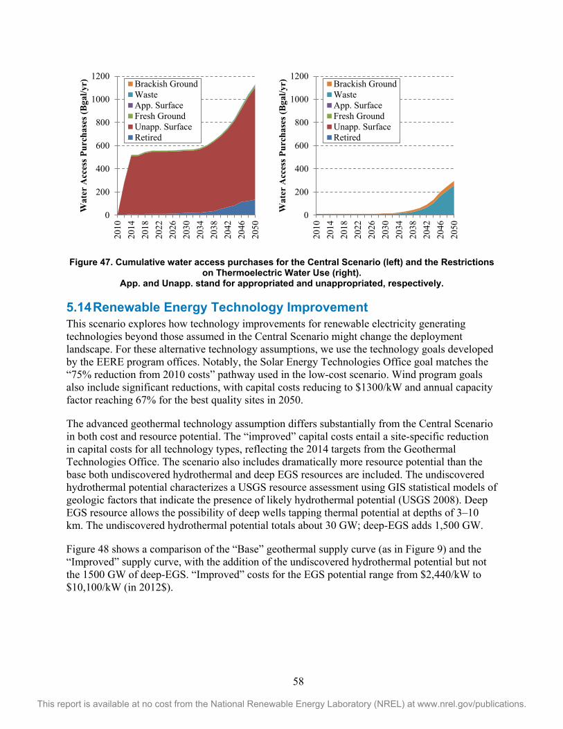
58


Figure 47. Cumulative water access purchases for the Central Scenario (left) and the Restrictions on Thermoelectric Water Use (right).

App. and Unapp. stand for appropriated and unappropriated, respectively.

5.14 Renewable Energy Technology Improvement This scenario explores how technology improvements for renewable electricity generating technologies beyond those assumed in the Central Scenario might change the deployment landscape. For these alternative technology assumptions, we use the technology goals developed by the EERE program offices. Notably, the Solar Energy Technologies Office goal matches the “75% reduction from 2010 costs” pathway used in the low-cost scenario. Wind program goals also include significant reductions, with capital costs reducing to $1300/kW and annual capacity factor reaching 67% for the best quality sites in 2050.

The advanced geothermal technology assumption differs substantially from the Central Scenario in both cost and resource potential. The “improved” capital costs entail a site-specific reduction in capital costs for all technology types, reflecting the 2014 targets from the Geothermal Technologies Office. The scenario also includes dramatically more resource potential than the base both undiscovered hydrothermal and deep EGS resources are included. The undiscovered hydrothermal potential characterizes a USGS resource assessment using GIS statistical models of geologic factors that indicate the presence of likely hydrothermal potential (USGS 2008). Deep EGS resource allows the possibility of deep wells tapping thermal potential at depths of 3–10 km. The undiscovered hydrothermal potential totals about 30 GW; deep-EGS adds 1,500 GW.

Figure 48 shows a comparison of the “Base” geothermal supply curve (as in Figure 9) and the “Improved” supply curve, with the addition of the undiscovered hydrothermal potential but not the 1500 GW of deep-EGS. “Improved” costs for the EGS potential range from $2,440/kW to $10,100/kW (in 2012$).

0

200

400

600

800

1000

1200

2010

2014

2018

2022

2026

2030

2034

2038

2042

2046

2050

Wat

er A

cces

s Pur

chas

es (B

gal/y

r)

Brackish GroundWasteApp. SurfaceFresh GroundUnapp. SurfaceRetired

0

200

400

600

800

1000

1200

2010

2014

2018

2022

2026

2030

2034

2038

2042

2046

2050

Wat

er A

cces

s Pur

chas

es (B

gal/y

r)

Brackish GroundWasteApp. SurfaceFresh GroundUnapp. SurfaceRetired

59


Figure 48. Comparison of "Base" and "Improved" geothermal resource supply curves.

Deep EGS resource is not included in this figure because the size of the resource distorts the figure to the point that the comparison is not useful. “Improved” costs for the 1,500 GW

of deep EGS resource range from $2440/kW to $10,100/kW (in 2012$).

As of this writing, there are no defined biopower or hydropower technology goals. In future years, we hope to make this scenario more robust and consistent across technologies.

Results Figure 49 shows how the input assumptions for the RE Technology Improvement Scenario impact renewable energy generation and CO2 emissions over time relative to the Central Scenario. The increased RE generation drives down CO2 emissions. Also, because the renewable energy technologies are lower-cost in this scenario compared to the Central Scenario, electricity prices are 5.6% lower than the Central Scenario in 2050. The increased renewable energy deployment also drives transmission builds, resulting in this scenario having 8.3% more transmission capacity in 2050 than the Central Scenario.

Figure 49. Renewable energy generation and CO2 emissions in the Central Scenario and the RE Technology Improvement Scenario.

0

5000

10000

15000

20000

25000

0 10 20 30 40 50

Capi

tal C

ost (

$/kW

)

Geothermal Resource Potential (GW)

Base

Improved

0

0.5

1

1.5

2

2.5

0

500

1000

1500

2000

2500

3000

3500

2010 2020 2030 2040 2050

CO

2 Em

issi

ons (

billi

on m

etri

c to

ns)

Ren

ewab

le E

nerg

y G

ener

atio

n (T

Wh)

Central ScenarioEERE Program Goals

CO2 Emissions

RE Generation

60


5.15 Nuclear Technology Breakthrough This scenario explores a future in which nuclear fission-generating technologies have growing public support and see increased technological advancement. Whereas the Central Scenario has a stable, high capital cost for new investments in nuclear generators—and therefore sees only token industry expansion—this scenario visits a future in which nuclear technologies costs decline substantially. In this scenario, the cost for new nuclear plants, including on green-field sites, falls steadily, and the industry regains, over time, a substantial market share of annual additions. The “Nuclear Breakthrough” scenario differs from the Central Scenario only by an alternative capital cost projection, shown in Figure 50, which is 40% below the AEO 2014 capital cost used for the rest of the scenarios.

Figure 50. Nuclear capital cost options

Results Figure 51 shows the change in generation that occurs in the Nuclear Technology Breakthrough Scenario compared to the Central Scenario. New nuclear plants begin to come online in the late 2020s, and nuclear generation grows to supply 30% of the total load by 2050. The increased presence of nuclear generators displaces all other generators types. Coal is the least affected, primarily because coal generation is already on the decline due to scheduled plant retirements. Compared to the Central Scenario, the Nuclear Technology Breakthrough Scenario leads to lower CO2 emissions, primarily through the displacement of natural gas generation.

0

1000

2000

3000

4000

5000

6000

2010 2020 2030 2040 2050

Nuc

lear

Ove

rnig

ht C

apit

al

Cost

($/k

W)

Baseline

Reduced

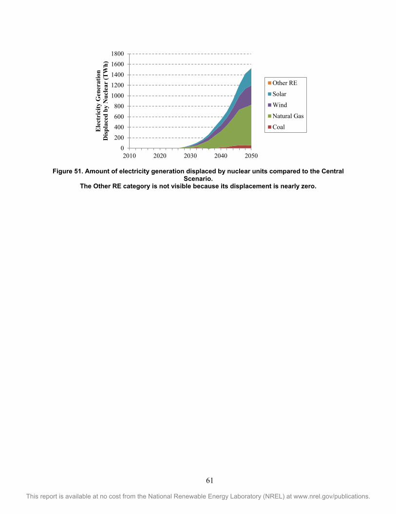
61


Figure 51. Amount of electricity generation displaced by nuclear units compared to the Central

Scenario. The Other RE category is not visible because its displacement is nearly zero.

0200400600800

10001200140016001800

2010 2020 2030 2040 2050

Ele

ctri

city

Gen

erat

ion

Dis

plac

ed b

y N

ucle

ar (T

Wh)

Other RE

Solar

Wind

Natural Gas

Coal

62


6 Discussion and Future Work This report—the first in an annual series—captures a range of sensitivities to a suite of drivers in the electric sector. This set of scenarios utilizes a consistent set of data and assumptions. Together, they establish a baseline understanding of the electric sector today as well as a range of projected pathways, and they form the basis for new studies and analysis. The 19 scenarios identify a range based on current understanding and projections; they do not represent predictions of how the electric sector will evolve. Rather, they map out likely trajectories within which the actual pathway may occur. Additionally, this report gives a basic description of the structure and assumption of the ReEDS model v.2015.1.

This report, coupled with the ATB, also provides a resource for analysts and decision makers interested in the current and future U.S. electricity system. The report and ATB will be updated on annually to provide the most relevant information available. For example, the DOE solar and water programs have ongoing analysis work that may inform new solar and hydropower cost projections for the 2016 release of this report.

Also, while there are high, mid and low forecasts for many technologies, there is an ongoing effort to assess the probability of attaining each forecast and working to normalize these forecasts across technologies in terms of probability of achieving them. For example, the “high cost” trajectory could be consistently 90% likely to be achieved while the “low cost” trajectory could be 25% likely to be achieved.

ReEDS is an electricity-sector-only model that has high geospatial resolution with the ability to capture many of the key factors for renewable electricity economics. The electricity sector has become increasingly complex with interactions across the meters (e.g., distributed generation, and demand response), across sectors (e.g., PHEVs and natural gas for other uses), and with anticipated clean energy policies (e.g., the proposed Clean Power Plan). ReEDS will continue to evolve to model these interactions effectively. For example, ongoing efforts are linking the ReEDS model to a distributed generation model (SolarDS), a natural gas supply chain model (Rice World Gas Trade Model [RWGTM[), and an economy-wide model (U.S. Regional Energy Policy [USREP]).

63


References Akhil, Abbas A, Georgianne Huff, Aileen B Currier, Benjamin C Kaun, Dan M Rastler, Stella

Bingqing Chen, Andrew L Cotter, Dale T Bradshaw, and William D Gauntlett. 2013. DOE/EPRI 2013 Electricity Storage Handbook in Collaboration with NRECA. SAND2013-5131. Albuquerque, NM: Sandia National Laboratory.

Augustine, C. 2011. Updated US Geothermal Supply Characterization and Representation for Market Penetration Model Input. TP-6A20-47459. Golden, CO: NREL.

Black & Veatch. 2012. Cost and Performance Data for Power Generation Technologies. Overland Park, KS: Black & Veatch Corporation.

Blair, Nate, Thomas Jenkin, James Milford, Walter Short, Patrick Sullivan, David Evans, Elliot Lieberman, et al. 2009. Renewable Energy and Efficiency Modeling Analysis Partnership: An Analysis of How Different Energy Models Addressed a Common High Renewable Energy Penetration Scenario in 2025. NREL/TP-6A2-45656. Golden, CO: NREL. http://escholarship.org/uc/item/9pv3r5fk.pdf.

CEC. 2009. Comparative Costs of California Central Station Electricity Generation Technologies, Draft Staff Report. CEC-200-2009-017-SD. California Energy Commission (CEC). http://www.energy.ca.gov/2009publications/CEC-200-2009-017/CEC-200-2009-017-SD.PDF.

Denholm, Paul, Erik Ela, Brendan Kirby, and Michael Milligan. 2010. The Role of Energy Storage with Renewable Electricity Generation. TP-6A2-47187. Golden, CO: NREL.

Denholm, Paul, Robert Mark Margolis, and Easan Drury. 2009. The Solar Deployment System (SolarDS) Model: Documentation and Sample Results. TP-6A2-45832. Golden, CO: National Renewable Energy Laboratory.

DOE. 2011. US Billion-Ton Update: Biomass Supply for a Bioenergy and Bioproducts Industry. ORNL/TM-2011/224. Agricultural and Biosystems Engineering Technical Reports and White Papers.

———. 2012. SunShot Vision Study. U.S. Department of Energy. EEI. 2009. 2008 Financial Review Plus 2009 Developments Annual Report of the U.S.

Shareholder-Owned Electric Utility Industry. Edison Electric Institute (EEI). http://www.eei.org/whatwedo/DataAnalysis/IndusFinanAnalysis/finreview/Documents/09_FinRevF.pdf.

———. 2010a. Transmission Project: At a Glance. Edison Electric Institute with assistance from Navigant Consulting, Inc.

———. 2010b. 2010 Q1 Rate Case Data. Edison Electric Institute (EEI). http://www.eei.org/whatwedo/DataAnalysis/IndusFinanAnalysis/Documents/2010_Q1_Rate_Case_Data.xls.

EIA. 2010. Annual Energy Outlook 2010. DOE/EIA-0383(2010). Washington, DC: U.S. DOE Energy Information Administration.

———. 2012. Annual Energy Outlook 2012. ———. 2013. Updated Capital Cost Estimates for Utility Scale Electricity Generating Plants.

Washington, DC: U.S. DOE Energy Information Administration. http://www.eia.gov/forecasts/capitalcost/pdf/updated_capcost.pdf.

———. 2014a. Annual Energy Outlook 2014. DOE/EIA-0383(2014). Washington, DC: US Energy Information Administration.

64


———. 2014b. The Electricity Market Module of the National Energy Modeling System: Model Documentation 2014. http://www.eia.gov/forecasts/aeo/nems/documentation/electricity/pdf/m068%282014%29.pdf.

———. 2014c. Monthly Energy Review. Washington, DC: Department of Energy. http://www.eia.gov/totalenergy/data/monthly/pdf/mer.pdf.

EIPC. 2012. Phase 2 Report: DOE Draft - Parts 2-7 Interregional Transmission Development and Analysis for Three Stakeholder Selected Scenarios. Eastern Interconnect Planning Collaborative. www.eipconline.com/uploads/20130103_Phase2Report_Part2_Final.pdf.

EnerNex. 2011. Eastern Wind Integration and Transmission Study. SR-5500-47078. Golden, CO: National Renewable Energy Laboratory.

EPA. 2014. “Carbon Pollution Emission Guidelines for Existing Stationary Sources: Electric Utility Generating Units.” https://federalregister.gov/a/2014-13726.

Feldman, David, Galen Barbose, Robert Margolis, Ted James, Samantha Weaver, Naim Darghouth, Ran Fu, Carolyn Davidson, Sam Booth, and Ryan Wiser. 2014. Photovoltaic System Pricing Trends: Historical, Recent, and Near-Term Projections 2014 Edition. NREL/PR-6A20-62558.

FERC. 2012. “FERC: Hydropower - General Information.” http://www.ferc.gov/industries/hydropower/gen-info.asp.

Gelman, R. 2013. Renewable Energy Data Book. Energy Efficiency & Renewable Energy (EERE). NREL Report No. BK-6A20-60197; DOE/GO-102013-4291. Golden, CO: National Renewable Energy Laboratory.

General Electric. 2010. Western Wind and Solar Integration Study. NREL/SR-550-47434. Golden, CO: National Renewable Energy Laboratory. http://www.nrel.gov/docs/fy10osti/47434.pdf.

GTM/SEIA. 2015. US Solar Market Insight Report: 2014 Year in Review. GTM & Solar Energy Industries Association (SEIA).

Habte, A., A. Lopez, M. Sengupta, and S. Wilcox. 2014. Temporal and Spatial Comparison of Gridded TMY, TDY, and TGY Data Sets. Golden, CO: National Renewable Energy Laboratory (NREL). http://www.osti.gov/scitech/biblio/1126297.

Hadjerioua, B., S.-C. Kao, R.A. McManamay, M.F.K. Pasha, D. Yeasmin, A.A. Oubeidillah, N.M. Samu, et al. 2013. An Assessment of Energy Potential from New Stream-Reach Development in the United States: Initial Report on Methodology. Oak Ridge, TN: Oak Ridge National Laboratory.

Hadjerioua, B., Yaxing Wei, and Shih-Chieh Kao. 2012. An Assessment of Energy Potential at Non-Powered Dams in the United States. Oak Ridge, TN: Oak Ridge National Laboratory.

Hall, Douglas G, Richard T Hunt, Kelly S Reeves, and Greg R Carroll. 2003. Estimation of Economic Parameters of US Hydropower Resources. INEEL/EXT-03-00662. Idaho Falls, ID: Idaho National Engineering and Environmental Laboratory. http://www1.eere.energy.gov/water/pdfs/doewater-00662.pdf.

Harper, John, Matt Karcher, and Mark Bolinger. 2007. Wind Project Financing Structures: A Review & Comparative Analysis. LBNL-63434.

Hostick, D., D.B. Belzer, S.W. Hadley, T. Markel, C. Marnay, and M. Kintner-Meyer. 2012. Renewable Electricity Futures Study Volume 3: End-Use Electricity Demand. NREL/TP-6A20-52409-3. National Renewable Energy Laboratory.

65


HSIP. 2012. Homeland Security Infrastructure Project. Jordan, Dirk C., and Sarah R. Kurtz. 2013. Photovoltaic Degradation Rates—an Analytical

Review. JA-5200-51664. Golden, CO: NREL. http://onlinelibrary.wiley.com/doi/10.1002/pip.1182/full.

Lantz, Eric, Ryan Wiser, and Maureen Hand. 2012. The Past and Future Cost of Wind Energy. CP-6A20-54526. Golden, CO: NREL. http://www.nrel.gov/docs/fy12osti/54526.pdf.

Logan, Jeffrey, Anthony Lopez, Trieu Mai, Carolyn Davidson, Morgan Bazilian, and Douglas Arent. 2013. “Natural Gas Scenarios in the US Power Sector.” Energy Economics 40: 183–95.

Lopez, Anthony, Billy Roberts, Donna Heimiller, Nate Blair, and Gian Porro. 2012. US Renewable Energy Technical Potentials: A GIS-Based Analysis. TP-6A20-51946. Golden, CO: NREL. http://cdn.decarboni.se/sites/default/files/publications/138258/US-renewable-energy-technical-potentials-GIS-based-analysis.pdf.

NETL. 2008. Recommended Project Finance Structures for the Economic Analysis of Fossil-Based Energy Projects. DOE/NETL-401/090808. National Energy Technology Laboratory (NETL). http://www.netl.doe.gov/energy-analyses/pubs/Project%20Finance%20Parameters%20-%20Final%20Report%20-%20Sept%202008_1.pdf.

North American Electric Reliability Corporation (NERC). 2010. 2010 Long-Term Reliability Assessment. http://www.nerc.com/files/2010%20LTRA.pdf.

NREL. 2010. “System Advisor Model (SAM) Version 2010.4.12.” https://www.nrel.gov/analysis/sam/.

———. 2012. Renewable Electricity Futures Study. Golden, CO: National Renewable Energy Laboratory.

———. 2015. “NREL Annual Technology Baseline (ATB).” http://www.nrel.gov/analysis/data_tech_baseline.html.

Saha, Amlan. 2013. Review of Coal Retirements. M.J. Bradley & Associates LLC. http://www.mjbradley.com/sites/default/files/Coal_Plant_Retirement_Review_Apr2013_0.pdf.

Short, Walter, Patrick Sullivan, Trieu Mai, Matthew Mowers, Caroline Uriarte, Nate Blair, Donna Heimiller, and Andrew Martinez. 2011. Regional Energy Deployment System (ReEDS). TP-6A20-46534. Golden, CO: NREL.

Sioshansi, Ramteen, and Paul Denholm. 2010. “The Value of Plug-in Hybrid Electric Vehicles as Grid Resources.” Energy Journal 31 (3): 1–23.

Stott, Brian, Jorge Jardim, and Ongun Alsaç. 2009. “DC Power Flow Revisited.” Power Systems, IEEE Transactions on 24 (3): 1290–1300.

Tegen, S., M. Hand, B. Maples, E. Lantz, P. Schwabe, and A. Smith. 2012. 2010 Cost of Wind Energy. TP-5000-52920. Golden, CO: NREL. http://www.idmarch.org/document_cache/bf7e00e30c994eed0e244043d5f29acd.pdf.

Tester, Jefferson W, Brian J Anderson, AS Batchelor, DD Blackwell, Ronald DiPippo, EM Drake, J Garnish, B Livesay, MC Moore, and K Nichols. 2006. The Future of Geothermal Energy. INL/EXT-06-11746. Idaho Falls, ID: Idaho National Laboratory.

USGS. 2008. Assessment of Moderate-and High-Temperature Geothermal Resources of the United States. U.S. Geological Survey. http://pubs.usgs.gov/fs/2008/3082/.

Vajjhala, Shalini P, and Paul S Fischbeck. 2007. “Quantifying Siting Difficulty: A Case Study of US Transmission Line Siting.” Energy Policy 35 (1): 650–71.

66


Ventyx. 2014. “Ventyx Velocity Suite.” http://www.ventyx.com/en/solutions/business-operations/business-products/velocity-suite.

Williams, Colin F, Marshall J Reed, and Robert H Mariner. 2008. A Review of Methods Applied by the US Geological Survey in the Assessment of Identified Geothermal Resources. 1296.

Wiser, Ryan, and Mark Bolinger. 2013. 2012 Wind Technologies Market Report. Wiser, Ryan, Eric Lantz, Mark Bolinger, and Maureen Hand. 2012. Recent Developments in the

Levelized Cost of Energy from Us Wind Power Projects. http://eaei.lbl.gov/sites/all/files/wind-energy-costs-2-2012_0.pdf.

Zavadil, Robert M, J. King, L. Xiadong, B. Lee, D. Moon, C. Finley, L. Alnes, et al. 2004. Xcel Energy and the Minnesota Department of Commerce, Wind Integration Study–Final Report. EnerNex Corporation and Wind Logics, Inc.

67


Appendix: Additional Scenario Output Plots This appendix presents comparative plots of the non-bidirectional scenarios. The plots are the same as those used for the bidirectional scenarios in Section 5.5, and they are provided so that readers can more fully compare the bidirectional scenarios with the non-bidirectional scenarios.

Figure 52. Annual wind generation in the non-bidirectional scenarios

Figure 53. Annual solar generation in the non-bidirectional scenarios. Solar generation includes CSP, distributed PV, and utility PV.

0

500

1000

1500

2000

2500

2010 2020 2030 2040 2050

Win

d G

ener

atio

n (T

Wh)

Central ScenarioVehicle ElectrificationCarbon CapPTC & ITC Extension80% National RPSClimate ChangeReduced RE ResourceBarriers to TransmissionRE Tech ImprovementsRestricted Cooling WaterNuke Tech Breakthrough

0

200

400

600

800

1000

1200

1400

1600

2010 2020 2030 2040 2050

Sola

r G

ener

atio

n (T

Wh)


68


Figure 54. Annual geothermal generation in the non-bidirectional scenarios. The RE Tech Improvements Scenario includes undiscovered hydrothermal and deep EGS

resources, while the other scenarios do not.

Figure 55. Annual hydropower generation in the non-bidirectional scenarios

0

50

100

150

200

250

300

350

400

2010 2020 2030 2040 2050

Geo

ther

mal

Gen

erat

ion

(TW

h) Central Scenario

Vehicle ElectrificationCarbon CapPTC & ITC Extension80% National RPSClimate ChangeReduced RE ResourceBarriers to TransmissionRE Tech ImprovementsRestricted Cooling WaterNuke Tech Breakthrough

270

290

310

330

350

370

390

2010 2020 2030 2040 2050

Hyd

ropo

wer

Gen

erat

ion

(TW

h) Central Scenario


69


Figure 56. Annual natural-gas-fired generation in the non-bidirectional scenarios

Figure 57. Annual nuclear generation in the non-bidirectional scenarios

0

500

1000

1500

2000

2500

2010 2020 2030 2040 2050

Nat

ural

Gas

Gen

erat

ion

(TW

h) Central Scenario


0

200

400

600

800

1000

1200

1400

1600

1800

2010 2020 2030 2040 2050

Nuc

lear

Gen

erat

ion

(TW

h)


70


Figure 58. Annual CO2 emissions from the power sector in the non-bidirectional scenarios

Figure 59. Cumulative AC transmission capacity in the non-bidirectional scenarios

0

0.5

1

1.5

2

2.5

2010 2020 2030 2040 2050

CO

2 Em

issi

ons (

billi

on m

etri

c to

ns)


80000

100000

120000

140000

160000

180000

200000

220000

240000

260000

2010 2020 2030 2040 2050

AC

Tra

nsm

issi

on (G

W-m

iles)


71


Figure 60. Retail electricity prices in the non-bidirectional scenarios

100105110115120125130135140145150

2010 2020 2030 2040 2050

Ele

ctri

city

Pri

ces (

2013

$/M

Wh)
