2016 hec-hms what is new - london workshop
TRANSCRIPT

1

2

3

4
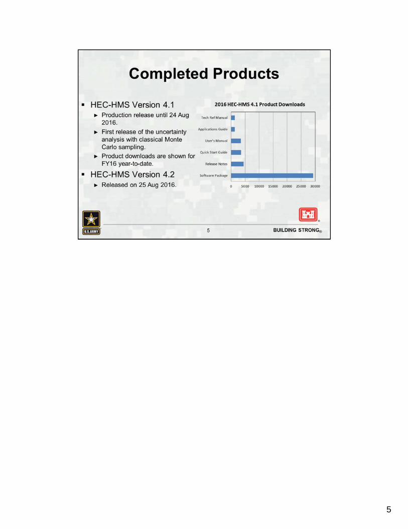
5

6
7
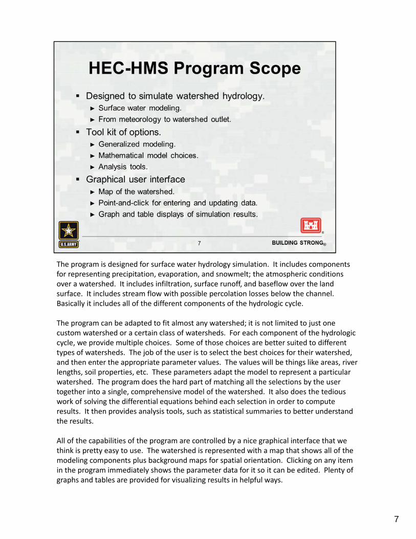
The program is designed for surface water hydrology simulation. It includes components for representing precipitation, evaporation, and snowmelt; the atmospheric conditions over a watershed. It includes infiltration, surface runoff, and baseflow over the land surface. It includes stream flow with possible percolation losses below the channel. Basically it includes all of the different components of the hydrologic cycle.
The program can be adapted to fit almost any watershed; it is not limited to just one custom watershed or a certain class of watersheds. For each component of the hydrologic cycle, we provide multiple choices. Some of those choices are better suited to different types of watersheds. The job of the user is to select the best choices for their watershed, and then enter the appropriate parameter values. The values will be things like areas, river lengths, soil properties, etc. These parameters adapt the model to represent a particular watershed. The program does the hard part of matching all the selections by the user together into a single, comprehensive model of the watershed. It also does the tedious work of solving the differential equations behind each selection in order to compute results. It then provides analysis tools, such as statistical summaries to better understand the results.
All of the capabilities of the program are controlled by a nice graphical interface that we think is pretty easy to use. The watershed is represented with a map that shows all of the modeling components plus background maps for spatial orientation. Clicking on any item in the program immediately shows the parameter data for it so it can be edited. Plenty of graphs and tables are provided for visualizing results in helpful ways.

8
Basin models, meteorological models, and control specifications are all main components used in simulation runs. The primary time‐series gages are precipitation and discharge; others used less often include temperature and solar radiation. A paired data function is simply a relationship between a dependent and independent variable; for example, storage‐discharge curves or rating curves. Also included in paired data are cross sections and annual patterns. Annual patterns are used for some special parameters that change value during the year, but use the same pattern for every year. Grid data can be boundary conditions like precipitation with a separate grid for each time interval in a time window, or they can be parameters like hydraulic conductivity.
Analysis tools are things that provide added value to simulations. That is, they start from a simple simulation run and then do additional processing. We will be adding more analysis tools in future versions of the program.
A project is stored in a directory on the file system. It can be created anywhere the user has permission to read and write, whether on the local computer or on a network share. When transferring a project the entire directory and its subdirectories should be sent.

9
This is the new interface first introduced with Version 3.0.0 in December 2005. Clicking on an item in the Watershed Explorer will load that editor in the bottom left Component Editor area, and if possible highlight it in the basin map (for hydrologic elements only). The Desktop area holds the basin map, global editors, and results. Any messages that are generated are scrolled continuously in the Message Log area.
The first tab (Components) of the Watershed explorer holds all of the different types of data in a project. The second tab (Compute) holds simulation items including simulation runs, optimization trials, and depth‐area analyses. The third tab (Results) provides access to any time‐series or summary result produced by all simulation items.

10
Data files are automatically added to the project directory as the user creates components and saves them. For example, there is a separate file for each basin model, meteorological model, and control specifications. There is one file that holds all of the time‐series gage information, one file that holds all of the paired data information, and one that holds all of the grid data information. Additional files are added to the project directory for other features as well. The user never needs to look in this files and should not edit the content.
DSS is central to the operation of HMS, but users do not need to be "experts" in DSS by any means. Any time‐series or paired data entered manually by the user is internally stored in a special DSS file in the project directory. Edits made by the user are automatically updated in the DSS file. Gage and paired data can also be retrieved from DSS by specifying a file and selecting a pathname. Because grid data is so complex, it cannot be entered manually but must be retrieved from a DSS file. All time‐series results during a simulation are stored in a DSS file and this is also how the program passes data internally. The results stored here can be used with other HEC products. Information in the User's Manual chapter 4 and appendix A explains the convention for pathnames.
Basin and meteorological models can be switched between U.S. customary and metric units. When switched, all parameter data is automatically converted between unit systems. Gages, paired data, and grid data each have their own unit system that can be what ever is most convenient. If a gage uses metric units but a basin model uses U.S. customary units, then a conversion happens automatically. Gage data is automatically interpolated if the simulation time interval is less than the data interval. Accumulation also happens automatically is gage data is at a shorter time interval than the simulation interval.

11
The basin model is where users spend most of their time. This is where the stream network is defined. Subbasins are the only elements that receive precipitation and other meteorological inputs. The are broken into segments for infiltration (loss rate), surface runoff (transform), and subsurface return flow (baseflow). Reaches represent the movement of water in an open channel. Reservoirs can be used for either natural lakes or man‐made dams; anything that impounds water. Junctions are a convenient way to show where multiple streams come together. Diversions are used lateral weirs, pumps stations, or other places were water is removed from the stream; diverted water can be connected back into the stream network at a downstream location. Sources are usually used as upstream boundary conditions when it is inconvenient to include the entire watershed in the basin model. Sinks are just a formal way of terminating a stream network; they are helpful when a basin model needs to contain more than one outlet perhaps because of multiple adjacent watersheds included in the same basin model.
The meteorological model handles all of the atmospheric conditions over the watershed. Precipitation is always required if there is a subbasin, but the other meteorological model elements are optional. Potential evapotranspiration is the upper limit on plant water use based only on atmospheric conditions. Elements within the basin model will use the potential evapotranspiration and then compute actual evapotranspiration based on available water in the soil and possibly other factors. When used, the snowmelt module takes the computed precipitation and determines if it fell in a liquid (rain) or frozen (snow) state. It then tracks the accumulation and melt of the snowpack.
Control specifications are lightweight components. They include the beginning date and time of a simulation, the ending date and time, and the time interval for calculations. Most model elements compute at the time interval specified in the control specifications. However, some elements use adaptive time stepping and may run as short as 1 second intervals. These special elements only record results at the specified time interval.

12
The basin map is used to visualize a basin model component. A variety of background map formats can be used including shape files, DXF, and aerial photos. The use of maps is always optional but can be helpful in gaining a spatial perspective to the watershed. Clicking on an element icon with the mouse will highlight it in the Watershed Explorer and display its data in the Component Editor. Only one basin model can be open at a time. You must click on the basin model in the Watershed Explorer for the map to open.

13

14

Modeling frameworks are needed that can capture knowledge uncertainty and natural variability uncertainty.
15

16L - 4.3/369/Scharffenberg

17L - 4.3/369/Scharffenberg

18L - 4.3/369/Scharffenberg

19L - 4.3/369/Scharffenberg

20L - 4.3/369/Scharffenberg
21

22
23
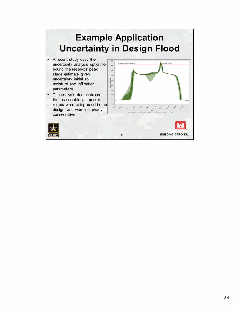
24
25

26

27

28

29
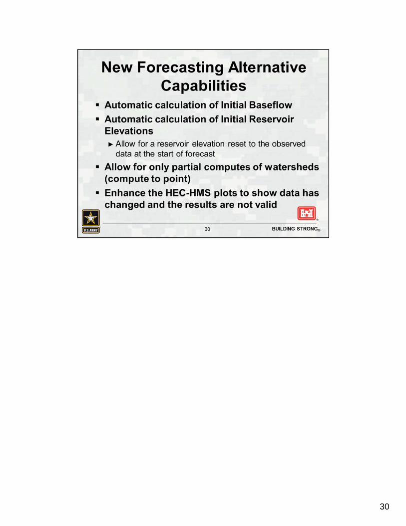
• When “Step” is selected, the difference between the observed and computed dischargeat the time of forecast is maintained throughout the remainder of the simulation. Therefore, if your computed results are 100 cfs below the observed flow at the time of forecast, then you’re going to maintain a difference of 100 cfs throughout the remainder of the simulation.
30

31

32

33

34

35
36

37

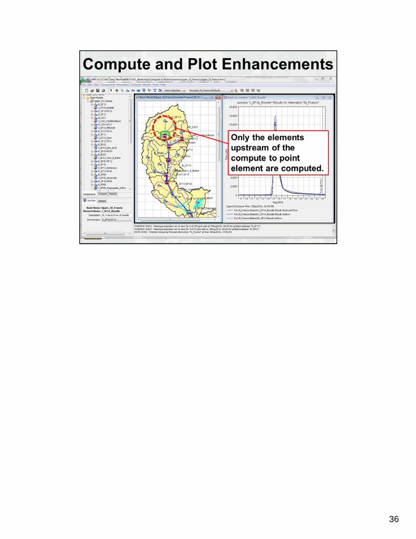
Additional Compute Efficiencies***Animated slide***Step by step of ho an upstream element can be changed and a compute to point downstream will only recompute the changed element and the dependent elements to the compute to point element. All of the independent elements that have not changed will use results from memory.
38

39

40

SubbasindelineationtoolsarebeingaddeddirectlytoHEC‐HMS ImportaGeoTiffterrainmodelandHEC‐HMSwillbeabletodelineatethe
subbasinandreachnetwork. IdentifyoutletpointsandHEC‐HMSwillsubdividethesubbasinandstream
network. WearerelyingonTauDEMforautomaticDEMprocessing.
41


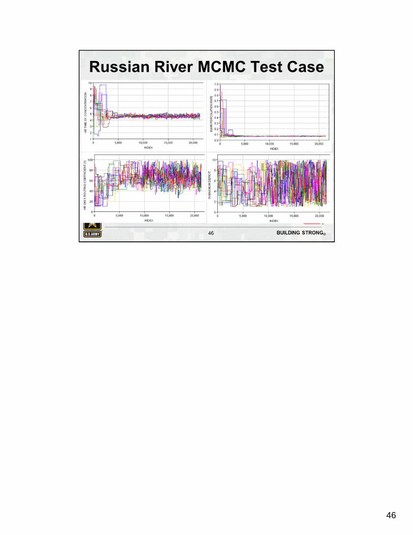
Run the chain to equilibrium (and this period is often referred to as the sampler burn‐in period) and subsequently sample from its stationary distribution.For a model of dimension size d (this might be an iterative process)
Specify a population size N – recommendation; N = an integer multiple of d; N=2 or N=2d
Initialize, using Latin Hypercube sampling, the sampling process (and the population), with Mo initial runs wherein Mo is >= 10d – recommend more if doable
Evolve the population and use the Metropolis jumping rule to accept jump proposals
Use a weight of evidence based approach to assess that the sampler is sampling with stable frequency (i.e., it is reached equilibrium and hence is sampling from the posterior distribution)
efficiency curvequantitative convergence diagnostic – necessary, but not sufficient conditiontrace plots(manual user intervention – to support this)
Once “converged”, save a thinned history of the monitoring period draws and use them for inference
43

44

The figures on this slide show computed and observed flow at the end of the MCMC simulation. The “best” parameter set has been selected. The 20,000+ model simulations, across multiple chains, were required to reach the optimal parameters.
45
46

47

The figures show the distribution of peak flow from the MCMC simulation.
48

49

50

• Unit hydrograph theory is the most commonly employed method within dam safety studies to transform excess precipitation to runoff at given locations in a dimensionless manner. In fact it’s recommended for use throughout the world in dam safety studies.
• According to Sherman, 1932, who originally proposed the unit hydrograph concept, the unit hydrograph of a watershed is “…the basin outflow resulting from one unit of direct runoff generated uniformly over the drainage area at a uniform rainfall rate during a specified period of rainfall duration.” This implies that the response of 2 inches of runoff over a given time is 2 times the response of 1 inches of runoff over the same amount of time.
• Unit hydrograph theory is still the state of the practice when it comes to hydrologic modeling. Take for instance analyses investigated parameter and modeling uncertainty: these often require many thousands of iterations that cannot be reasonably executed using more complicated runoff routing techniques. These analyses almost always are performed using unit hydrograph theory.
51

• However, due to differences hydraulic reactions between large and small precipitation events, the corresponding unit hydrographs have not been found to be equal, as implied by unit hydrograph theory.
• Minshall was one of the first people to explore the different runoff hydrographs that result from differing intensities of precipitation. The graph shown here is from his classic report in 1960. He showed that as precipitation intensity increases, runoff tends to peak sooner in time and has greater peak flow rates. This is due to greater depths in the stream channels and overland planes; as water depth increases, effective roughness decreases leading to shorter travel times, etc.
52

• The amount of precipitation excess contained within the most intense precipitation event of recent history in the Ball Mountain Dam watershed absolutely PALES in comparison to the Probable Maximum Precipitation.
• Using calibrated unit hydrograph transform parameters from the Aug 2011 event (and really any other event that has available data) can lead to errors when trying to route excess precipitation on the order of 4 inches/hour.
53

• An HEC‐HMS and HEC‐RAS model were created for the area upstream of Ball Mountain Dam. Both models used the same modeling domain extents and were calibrated using the largest inflow events to Ball Mountain Dam.
54

• The effect of precipitation intensity on runoff timing and magnitude were evaluated using the previously mentioned HEC‐RAS 2D model. Unit hydrograph theory assumes that the hydrograph ordinates of a 2 inch runoff event are two times larger than a 1 inch runoff event. This assumption of linearity can be evaluated using hydrodynamic models which include the physical processes that govern how water flows over the land surface.
• To demonstrate the non‐linear effects of increasingly large rainfall excess values, two, three, four, five, six, seven, and eight inches of excess precipitation were input to the HEC‐RAS 2D model over a unit duration (i.e. 1‐hr). The overland roughness parameters from the Aug 2011 and Unit Hydrograph simulations were compiled using weighted averages to create a parameter dataset for use in these simulations. The resulting hydrographs were then extracted at the “outlet” cell faces just upstream of the Ball Mountain Dam reservoir. Each ordinate of the hydrographs was then divided by the input excess precipitation amount to “normalize” the runoff response.
55

• If one were solely interested in predicting the peak flow rate of the PMF, it may be useful to compare the peak flow rates of the unit hydrographs and the normalized storm hydrographs estimated using the HEC‐RAS 2D model. For instance, dividing the peak flow rate of the 2 inch/hour normalized storm by the HEC‐RAS 1‐hour unit hydrograph peak flow rate results in a ratio of 1.12. Similarly, dividing the peak flow rate of the 5 inch/hour normalized storm by the 1‐hour unit hydrograph peak flow rate results in a ratio of 2.12.
• This table demonstrates that increasingly large unit hydrograph peaking factors are needed to achieve the same peak flow rate as the normalized storm depth (i.e. precipitation excess rate) increases. However, using excessively large unit hydrograph peaking factors may result in hydrologic modeling parameters that are physically unrealistic.
56

57

58

59

60

61

62
63

64

65