2017 center for opportunity urbanism (cou) standard of ... · included. 2. the bea rpps, as...

POLICY BRIEF

The Center for Opportunity Urbanism (COU)

Standard of Living Index 2nd Annual Edition

December 2017

By Wendell Cox, Senior Fellow

2017 COU Standard of Living Index The Center for Opportunity Urbanism (COU) Standard of Living Index estimates the earnings necessary for an average standard of living for new movers to metropolitan areas. It assumes that these new residents would either rent the average priced apartment or purchase the average priced house, on typical terms, the percentages reflecting the share of owned and rented occupied units in the United States. Estimates are provided for the 107metropolitan areas (cities) with more than 500,000 population. This is the second annual edition, and contains estimates for 2016. In recent decades, the differential in costs of living between U.S. metropolitan areas have increased substantially. Much of this difference reflects a historical divergence in housing costs between metropolitan areas. Housing cost differentials have become so significant that in 2011 the Census Bureau began publishing the "Supplemental Poverty Measure," which adjusts poverty data for a single item of cost, rents. However, the substantial divergence between metropolitan areas in the costs of owned housing in are not reflected in data includes only rents. The purpose of the COU Standard of Living Index is value the annual earnings for the average employee in each metropolitan area based on a cost of living measure that reflects variations from national costs reflecting both renting and house purchases (see: "Methodology Appendix"). The COU Standard of Living Index is also intended to provide corporate relocation professionals with comprehensive information on the cost of living competitiveness, which is an important consideration in comparing labor market1 factors. The leading cost of living index in the United States is the U.S. Department of Commerce, Bureau of Economic Analysis Regional Price Parities (RPPs) The latest edition of which provides 2015 data for the states and metropolitan areas. The first publication of RPPs occurred in 2008. The RPPs are divided into three cost categories, goods, rents and services other than rents. The BEA RPPs do not currently include the costs of owned housing, though eventually it is intended that this will be

1 Labor markets are metropolitan areas.

2nd Annual COU Standard of Living Index (2016 data) 1

http://www.opportunityurbanism.org/

included.2The BEA RPPs, as adjusted for 2016,is referred to as the "Renter Cost of Living Index,” The Renter Cost of Living Index is combined with the COU "Current Purchaser Cost of Living Index of Living Index, at weights that reflect the national rental and home ownership rate, to obtain the COU Composite Cost of Living Index. This measure is used to adjust nominal pay per job in each metropolitan area to obtain "real" (cost of living adjusted) pay per job. The differences in real pay per job compared to the national average produce the standard of living variations and the COU Standard of Living Index for each metropolitan area. Metropolitan Areas with the Highest and Lowest Standards of Living Overall, the average pay per job in the United States was $53,600. When adjusted by the COU Composite Cost of Living Index, the national pay per job is estimated at $48,800.3 This figure is considered the national average standard of living (a COU Standard of Living Index of 100.0). Metropolitan Areas with Highest COU Standard of Living Index: San Jose has the highest cost of living adjusted pay per job among the 107 metropolitan areas ($67,500). San Jose contains much of the Silicon Valley, the world’s leading information technology hub. This pay per job indicates the highest standard of living, 39 percent above the national average of $48,800. Nonetheless, this is considerably below San Jose's average pay of $116,900 before the cost of living adjustment. The difference between these who figures is principally the much higher cost of housing in San Jose, the least affordable major market in the United States and rated as fifth least affordable in the Demographia International Housing Affordability Survey.4 Even so, San Jose holds the top position by a 13 percent margin or $9,000 over second ranked Houston. This is by far the largest monetary difference between among the 107 metropolitan areas ranked (Figure 1). Detailed data is shown in Tables 1 and 2. In contrast, Houston has an average real pay per job of $58,400, where the average cost of living adjusted pay indicates a COU Standard of Living Index 20 percent above the national average 0f $48,800. Durham, North Carolina, Atlanta 2Bettina Aten, Eric Figueroa and Troy Martin, “How can the American Community Survey (ACS) be used to improve the imputation of Owner-Occupied Rent Expenditures?," United States Department of Commerce, Bureau of Economic Analysis, 2011, http://www.bea.gov/papers/pdf/WP_ACS_OORE_020112.pdf. 3 $56,321 is adjusted by the COU "Current Purchaser Cost of Living Index (116.1) to obtain the $46,410 standard of living benchmark. The Current Purchaser Cost of Living Index of living index is based on the BEA RPP of 100.0 (Renter Cost of Living Index). 413th Annual Demographia International Housing Affordability Survey, http://www.demographia.com/dhi.pdf.

$0 $10,000 $20,000 $30,000 $40,000 $50,000 $60,000 $70,000

UNITED STATES AVERAGESt. Louis,, MO-IL

San Francisco, CAMemphis, TN-MS-AR

Pittsburgh, PACleveland, OH

Minneapolis-St. Paul, MN-WIWashington, DC-VA-MD-WV

Birmingham, ALCincinnati, OH-KY-IN

Charlotte, NC-SCDallas-Fort Worth, TX

Seattle, WAHartford, CT

Boston, MA-NHDetroit, MI

Bridgeport-Stamford, CTAtlanta, GA

Durham, NCHouston, TX

San Jose, CA

Estimated Real Pay Per Job 2016

COU Standard of Living Index: Top 20METROPOLITAN AREAS OVER 500,000

Figure 1

Same scale asFigure 2 forcomparison

Estimated: See Text.


http://www.bea.gov/papers/pdf/WP_ACS_OORE_020112.pdf

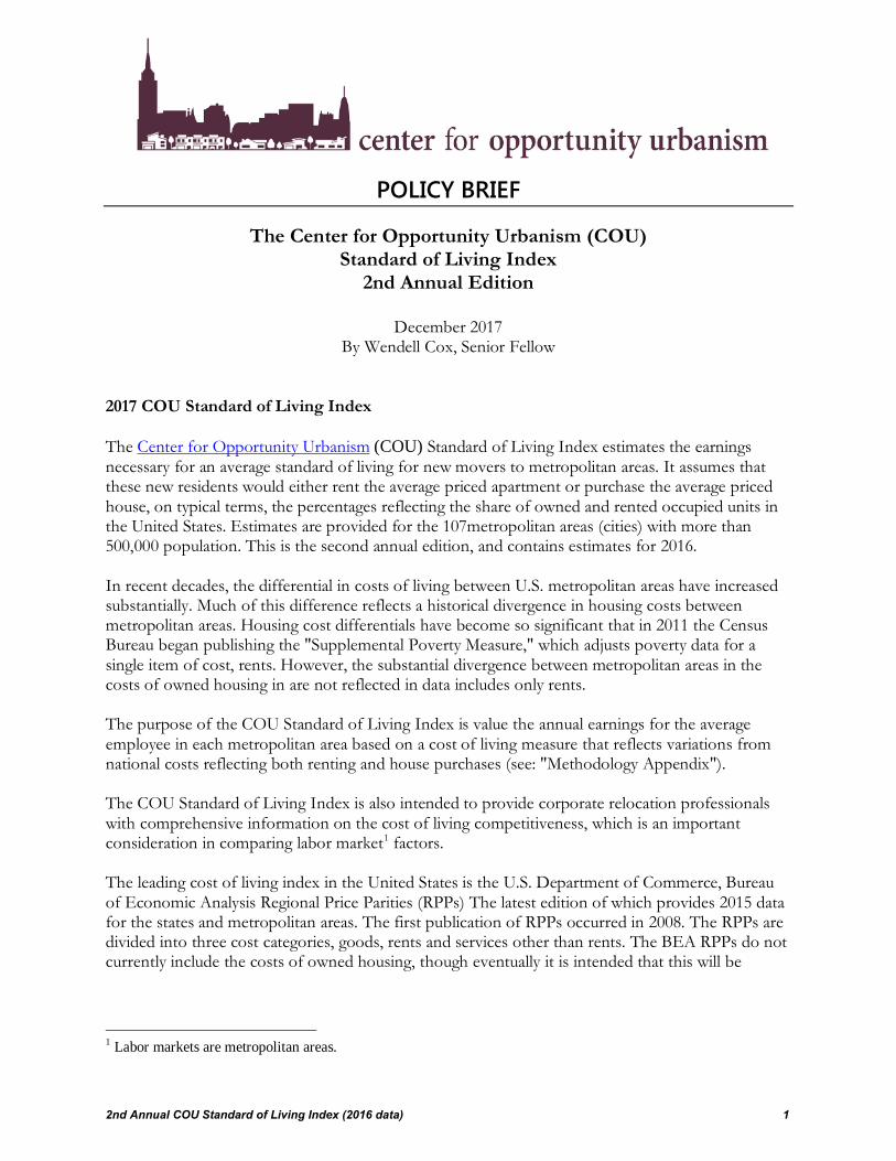
and Bridgeport – Stamford, Connecticut, which ranked as the third, fourth and fifth highest real pay per job and COU Standard of Living Index. Detroit ranks sixth, followed by Boston, Seattle, Hartford and Charlotte. All but two of the top 20 cities have more than 1 million population, while Durham and Bridgeport-Stamford have populations between 500,000 and 1,000,000. Ten of the top 20 cities are in the South, 4 in the Midwest and three each in the Northeast and West. There have been only modest changes in the rankings of the most affluent metropolitan over the past year. The top three, San Jose, Houston and Durham, remain the same as last year. Atlanta moved from seventh most affluent to fourth, trading places with Bridgeport-Stamford, now ranked fifth. There were other changes in the second five top metropolitan areas. However, despite the ranking changes, the 10 most affluent urban areas included the same metropolitan areas as in 2015. Metropolitan Areas with Lowest COU Standard of Living Index: Honolulu has the lowest cost of living adjusted pay per job, at $32,000 per job. Honolulu's COU Standard of Living Index is approximately 33 percent below the national average of $48,800. Honolulu, is joined by all three metropolitan areas in the Los Angeles combined statistical area5 (Los Angeles, Riverside-San Bernardino and Oxnard), as well as Ogden (UT), Fresno (CA) and Santa Rosa (CA). McAllen (TX), Daytona Beach (FL), McAllen (TX) and Sarasota (FL) are the only metropolitan areas in the bottom ten from outside the West (Figure 2). Honolulu and Santa Rosa were ranked with the lowest pay per job and COU Standard of Living Index for the second straight year. Daytona Beach fell to third least affluent from fourth place last year, while Riverside-San Bernardino from fifth least affluent to fourth. McAllen, ranked third least affluent in 2015, improved to fifth least affluent. There was one new entrant to the 10 least affluent metropolitan areas, Sarasota, which replaced El Paso. The Widening Cost of Living Differences Between Metropolitan Areas The cost of housing represents the largest difference in the cost of living between U.S. metropolitan areas.

5 A combined statistical area is a broader metropolitan area consisting of adjacent metropolitan areas that meet commuting criteria established by the Office of Management and Budget.

$0 $10,000 $20,000 $30,000 $40,000 $50,000 $60,000 $70,000

UNITED STATESHonolulu, HI

Santa Rosa, CADaytona Beach, FL

Riverside-San Bernardino, CAMcAllen, TXOxnard, CAFresno, CA

Los Angeles, CAOgden, UT

Sarasota, FLProvo, UT

El Paso, TXStockton, CA

Cape Coral, FLPortland, ME

San Diego, CAModesto, CA

Lancaster, PAScranton, PA

Youngstown, OH-PA

Estimated Real Pay Per Job 2016

COU Standard of Living Index: Bottom 20METROPOLITAN AREAS OVER 500,000

Figure 2




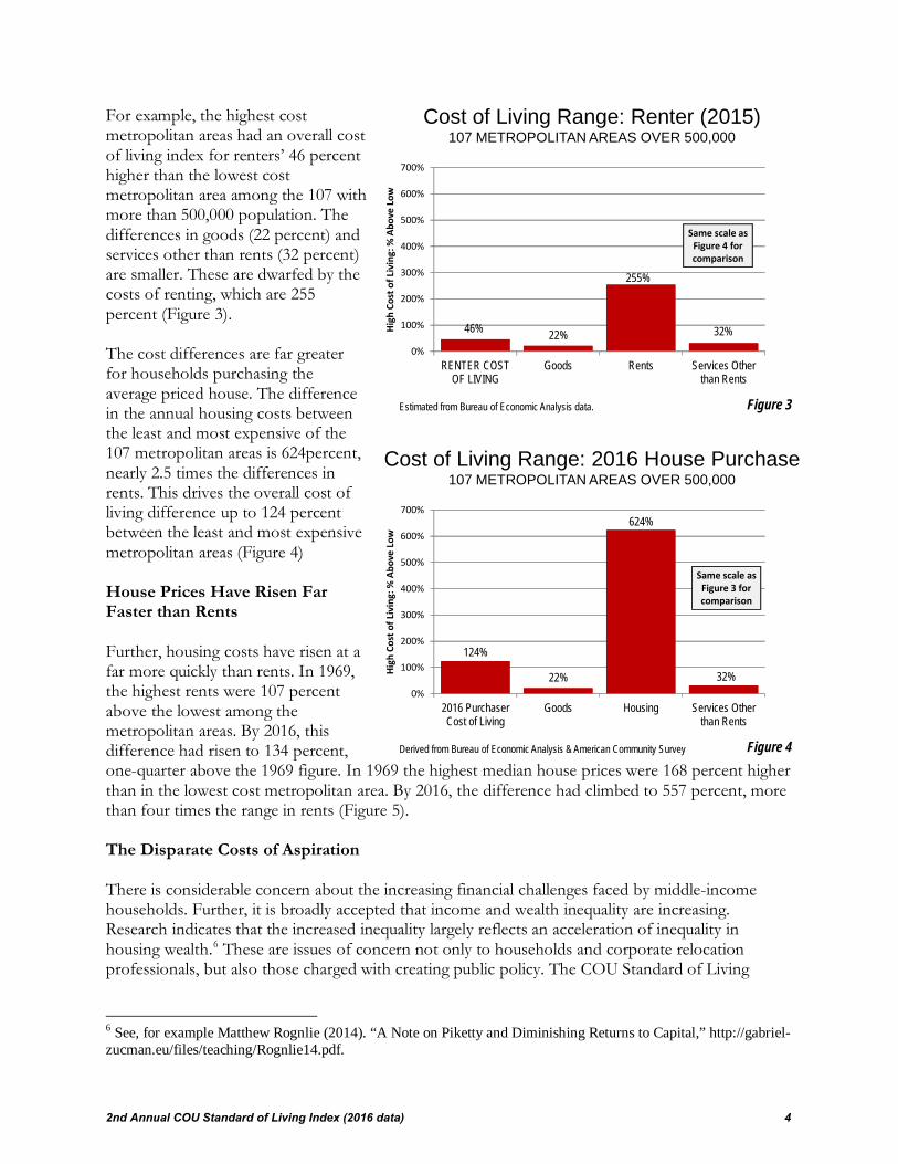
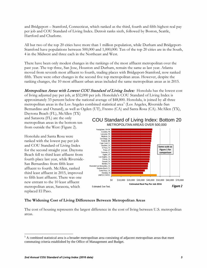
For example, the highest cost metropolitan areas had an overall cost of living index for renters’ 46 percent higher than the lowest cost metropolitan area among the 107 with more than 500,000 population. The differences in goods (22 percent) and services other than rents (32 percent) are smaller. These are dwarfed by the costs of renting, which are 255 percent (Figure 3). The cost differences are far greater for households purchasing the average priced house. The difference in the annual housing costs between the least and most expensive of the 107 metropolitan areas is 624percent, nearly 2.5 times the differences in rents. This drives the overall cost of living difference up to 124 percent between the least and most expensive metropolitan areas (Figure 4) House Prices Have Risen Far Faster than Rents Further, housing costs have risen at a far more quickly than rents. In 1969, the highest rents were 107 percent above the lowest among the metropolitan areas. By 2016, this difference had risen to 134 percent, one-quarter above the 1969 figure. In 1969 the highest median house prices were 168 percent higher than in the lowest cost metropolitan area. By 2016, the difference had climbed to 557 percent, more than four times the range in rents (Figure 5). The Disparate Costs of Aspiration There is considerable concern about the increasing financial challenges faced by middle-income households. Further, it is broadly accepted that income and wealth inequality are increasing. Research indicates that the increased inequality largely reflects an acceleration of inequality in housing wealth.6 These are issues of concern not only to households and corporate relocation professionals, but also those charged with creating public policy. The COU Standard of Living

6 See, for example Matthew Rognlie (2014). “A Note on Piketty and Diminishing Returns to Capital,” http://gabriel-zucman.eu/files/teaching/Rognlie14.pdf.

46% 22%

255%

32%0%

100%

200%

300%

400%

500%

600%

700%

RENTER COST OF LIVING

Goods Rents Services Other than Rents

High

Cos

t of L

ivin

g: %

Abo

ve L

ow

Estimated from Bureau of Economic Analysis data. Figure 3


Cost of Living Range: Renter (2015)107 METROPOLITAN AREAS OVER 500,000

124%

22%

624%

32%0%

100%

200%

300%

400%

500%

600%

700%

2016 Purchaser Cost of Living

Goods Housing Services Other than Rents

High

Cos

t of L

ivin

g: %

Abo

ve L

ow

Derived from Bureau of Economic Analysis & American Community Survey Figure 4

Cost of Living Range: 2016 House Purchase107 METROPOLITAN AREAS OVER 500,000



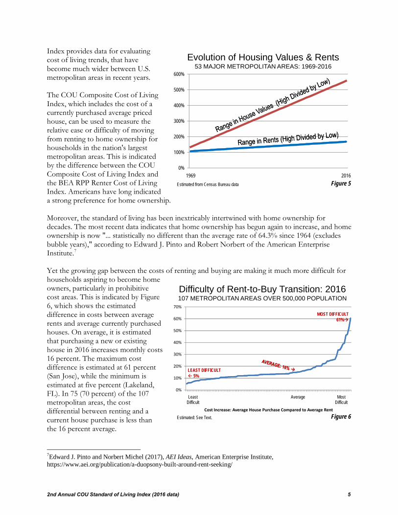
Index provides data for evaluating cost of living trends, that have become much wider between U.S. metropolitan areas in recent years. The COU Composite Cost of Living Index, which includes the cost of a currently purchased average priced house, can be used to measure the relative ease or difficulty of moving from renting to home ownership for households in the nation's largest metropolitan areas. This is indicated by the difference between the COU Composite Cost of Living Index and the BEA RPP Renter Cost of Living Index. Americans have long indicated a strong preference for home ownership. Moreover, the standard of living has been inextricably intertwined with home ownership for decades. The most recent data indicates that home ownership has begun again to increase, and home ownership is now "... statistically no different than the average rate of 64.3% since 1964 (excludes bubble years)," according to Edward J. Pinto and Robert Norbert of the American Enterprise Institute.7 Yet the growing gap between the costs of renting and buying are making it much more difficult for households aspiring to become home owners, particularly in prohibitive cost areas. This is indicated by Figure 6, which shows the estimated difference in costs between average rents and average currently purchased houses. On average, it is estimated that purchasing a new or existing house in 2016 increases monthly costs 16 percent. The maximum cost difference is estimated at 61 percent (San Jose), while the minimum is estimated at five percent (Lakeland, FL). In 75 (70 percent) of the 107 metropolitan areas, the cost differential between renting and a current house purchase is less than the 16 percent average. 7Edward J. Pinto and Norbert Michel (2017), AEI Ideas, American Enterprise Institute, https://www.aei.org/publication/a-duopsony-built-around-rent-seeking/

0%

100%

200%

300%

400%

500%

600%

1969 2016

Evolution of Housing Values & Rents53 MAJOR METROPOLITAN AREAS: 1969-2016

Estimated from Census Bureau data Figure 5

0%

10%

20%

30%

40%

50%

60%

70%

Least Difficult

Average Most Difficult

Cost Increase: Average House Purchase Compared to Average Rent

Difficulty of Rent-to-Buy Transition: 2016107 METROPOLITAN AREAS OVER 500,000 POPULATION

Figure 6Estimated: See Text.

LEAST DIFFICULT 5%

MOST DIFFICULT61%


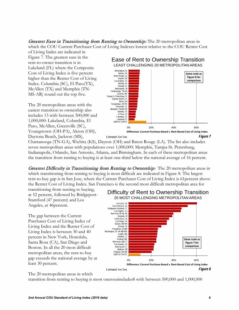
Greatest Ease in Transitioning from Renting to Ownership: The 20 metropolitan areas in which the COU Current Purchaser Cost of Living Indexes lowest relative to the COU Renter Cost of Living Index are indicated in Figure 7. The greatest ease in the rent-to-owner transition is in Lakeland (FL) where the Composite Cost of Living Index is five percent higher than the Renter Cost of Living Index. Columbia (SC), El Paso(TX), McAllen (TX) and Memphis (TN-MS-AR) round out the top five. The 20 metropolitan areas with the easiest transition to ownership also includes 13 with between 500,000 and 1,000,000: Lakeland, Columbia, El Paso, McAllen, Greenville (SC), Youngstown (OH-PA), Akron (OH), Daytona Beach, Jackson (MS), Chattanooga (TN-GA), Wichita (KS), Dayton (OH) and Baton Rouge (LA). The list also includes seven metropolitan areas with populations over 1,000,000: Memphis, Tampa-St. Petersburg, Indianapolis, Orlando, San Antonio, Atlanta, and Birmingham. In each of these metropolitan areas the transition from renting to buying is at least one-third below the national average of 16 percent. Greatest Difficulty in Transitioning from Renting to Ownership: The 20 metropolitan areas in which transitioning from renting to buying is most difficult are indicated in Figure 8. The largest rent-to-buy gap is in San Jose, where the Current Purchaser Cost of Living Index is 61percent above the Renter Cost of Living Index. San Francisco is the second most difficult metropolitan area for transitioning from renting to buying, at 52 percent, followed by Bridgeport-Stamford (47 percent) and Los Angeles, at 46percent. The gap between the Current Purchaser Cost of Living Index of Living Index and the Renter Cost of Living Index is between 30 and 40 percent in New York, Honolulu, Santa Rosa (CA), San Diego and Boston. In all the 20 most difficult metropolitan areas, the rent-to-buy gap exceeds the national average by at least 30 percent. The 20 metropolitan areas in which transition from renting to buying is most onerousincludes8 with between 500,000 and 1,000,000

0% 20% 40% 60%

UNITED STATESLakeland, FL

Columbia, SCEl Paso, TXMcAllen, TX

Memphis, TN-MS-ARGreenville, SC

Youngstown, OH-PAAkron, OH

Daytona Beach, FLTampa-St. Petersburg, FL

Jackson, MSChattanooga, TN-GA

Indianapolis. INOrlando, FLWichita, KS

San Antonio, TXDayton, OH

Baton Rouge, LAAtlanta, GA

Birmingham, AL

Difference: Current Purchase-Based v. Rent-Based Cost of Living Index

Ease of Rent to Ownership TransitionLEAST CHALLENGING 20 METROPOLITAN AREAS

Figure 7



0% 20% 40% 60%

UNITED STATESPortland, OR-WA

Madison, WINew Haven CT

Sacramento, CAWorcester, MA-CT

Portland, MEHartford, CTSeattle, WA

Washington, DC-VA-MD-WVProvidence, RI-MA

Oxnard, CABoston, MA-NHSan Diego, CA

Santa Rosa, CAHonolulu, HI

New York, NY-NJ-PALos Angeles, CA

Bridgeport-Stamford, CTSan Francisco, CA

San Jose, CA

Difference: Current Purchase-Based v. Rent-Based Cost of Living Index

Figure 8



Difficulty of Rent to Ownership Transition20 MOST CHALLENGING METROPOLITAN AREAS


population: Bridgeport, Honolulu, Santa Rosa, Oxnard, Portland (ME), Worcester, New Haven (CT) and Madison (WI). There are also 12 metropolitan areas with populations over 1,000,000: San Francisco, San Jose, Los Angeles, New York, San Diego, Boston, Providence, Washington, Seattle, Hartford, Sacramento and Portland (OR). In each of these metropolitan areas the transition from renting to buying is at least 30 percent higher the national average of 16 percent. A Changing Geography of Opportunity The cost of living has emerged as a major factor in net domestic migration between the nation's metropolitan areas. Households moving within the United States are drawn to areas with lower costs of living, as is indicated in Figure 9. Between 2010 and 2016, there was a net domestic migration loss of 1,477,000 residents from the metropolitan areas with higher than average COU Composite Costs of Living (109.8). In contrast, there was net domestic migration gain of 2,043,000 to the metropolitan areas with lower than average costs of living.8In addition, the rate of domestic migration tends to be higher where the cost of living is lower (as measured by the COU Composite Cost of Living Index). Table 3 provides a summary of the domestic migration data as related to the cost of living. This finding, that people are moving generally to lower cost areas from higher cost areas is consistent with the research findings of various academic studies.9 Methodology Appendix The COU Standard of Living Index rates the nation’s 107 metropolitan areas (cities) with more than 500,000 population based on average pay per job adjusted for the cost of living. Pay per Job data is from the US Department of Labor Bureau of Labor Statistics for 2016, which is adjusted for metropolitan area cost of living differences using the COU Composite Cost of Living Index, as follows.

8 The balance, a net domestic migration loss of 566,000 was experienced in areas outside the 107 largest metropolitan areas. 9 See, for example, Edward L Glaeser and Joseph Gyourko (2017), “The Economic Implications of Housing Supply, Samuel Zell and Robert Lurie Real Estate Center, University of Pennsylvania. http://realestate.wharton.upenn.edu/research/papers.php?paper=802 and Peter Ganong and Daniel Shoag, “Why Has Regional Income Convergence in the U.S. Declined?”HKS Working Paper No. RWP12-028, 2013. http://papers.ssrn.com/sol3/Delivery.cfm/SSRN_ID2241069_code1638787.pdf?abstractid=2081216&mirid=5.

-1,500,000

-1,000,000

-500,000

0

500,000

1,000,000

1,500,000

-25% & Lower

-25% to -5% -5% to 0% 0% to +5% +5% to +25%

25% & Higher

By Variation from COU Composite Cost of Living Index Figure 9

Net Domestic Migration by Cost of Living2010-2016: 107 METROPOLITAN AREAS

Estimated: See Text and Table 3.


http://papers.ssrn.com/sol3/Delivery.cfm/SSRN_ID2241069_code1638787.pdf?abstractid=2081216&mirid=5

(a) The cost of living for renters is based on the US Department of Commerce Bureau of Economic Analysis (BEA) Regional Price Parities for 2015. Relative weights are modeled for the three components (goods, rents and services other than rents) The rent component is adjusted in each metropolitan area for the change relative to the national average between 2015 and 2016 using rents (average gross rents), using American Community Survey data. In this calculation, the national rent weight is held constant, as are the weights for goods and other services. The result is the COU estimated "Renter Cost of Living Index” for 2016. (b) The cost of living for current (2106) home purchasers is estimated by substituting ownership costs for the cost of renting, using American Community Survey data. It is assumed that the current home purchase involves an average priced house, with a down payment of 14 percent, financed by a 30-year fixed rate mortgage at 3.65 percent10 interest with mortgage insurance. Other current home purchase costs such as insurance, real estate taxes and home owner association or condominium fees are estimated from the American Community Survey. The result is the COU estimated "Current Purchaser Cost of Living Index of Living Index” for 2016.

(c) The Renter Cost of Living Index and the Current Purchaser Cost of Living Index of Living Index are weighted based on the national distribution of 63.1 percent homeowners and 36.9 percent renters,11 to estimate the COU Composite Cost of Living Index.12 (d) Real pay per job is obtained by dividing the nominal pay per job by the COU Composite Cost of Living Index. The national real pay per job is the national standard of living average. (e)The COU Standard of Living Index is obtained by dividing the real pay per job by the national standard of living average.

The COU Composite Cost of Living Index is based on estimates of recurring monthly or annual expense, and does not include provision for down payments for owned houses or for "points" that are not included in monthly mortgage payments. There is more to the standard of living than money: The COU Standard of Living is offered with the realization that there is more to the standard of living than money. However, costs provide an objective measure of what households can buy. Moreover, much of middle-income America struggles to "make ends meet," and prices differences are important. As incomes rise, the standard of living may be determined to a lesser degree by income. Caveat and need for refinements: The COU Standard of Living Index is based on the COU Composite Cost of Living Index. The COU composite cost of living index is thus not a general cost of living index, but rather is focused on the need to comprehensively compare costs of living

10 2016 annual rate from 30-Year Fixed-Rate Mortgages Since 1971, Freddie Mac, http://www.freddiemac.com/pmms/pmms30.html. 11 Calculated from the American Community Survey, 2016. 12 The COU Composite Cost of Living does not measure the overall costs for households renting and buying, but rather households that rent and buy with typical purchase terms in the current year. An index indicating overall costs of home ownership, regardless of the home purchase date would indicate lower values and does not currently exist.


between metropolitan areas by households considering a geographical move and firms considering relocation. It is likely that the actual cost of living is underestimated in some more expensive metropolitan areas. Neither BEA's cost of living index (RPPs) nor the COU Composite Cost of Living Index includes personal taxes, such as federal, state and local income taxes.13 The federal income tax is progressive, such that higher rates are paid with higher incomes. This is also true of some state and local income taxes. As a result, residents in metropolitan areas with higher nominal average pay and prohibitive costs of living are likely to pay more in taxes, further discounting the value of their earnings. It is to be hoped that useful metrics will be developed that make even more reflective cost of living indexes possible.

13 Bureau of Economic Analysis, Frequently Asked Questions: What is included in personal taxes? http://www.bea.gov/faq/index.cfm?faq_id=550


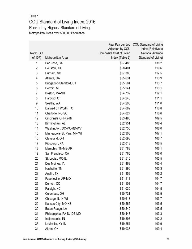
Table 1

COU Standard of Living Index: 2016Ranked by Highest Standard of LivingMetropolitan Areas over 500,000 Population

Rank (Out of 107) Metropolitan Area

Real Pay per Job Adjusted by COU

Composite Cost of Living

Index (Table 2)

COU Standard of Living Index (Relative to

National Average

Standard of Living)

1 San Jose, CA $67,485 138.2

2 Houston, TX $58,401 119.6

3 Durham, NC $57,380 117.5

4 Atlanta, GA $55,631 113.9

5 Bridgeport-Stamford, CT $55,504 113.7

6 Detroit, MI $55,241 113.1

7 Boston, MA-NH $54,732 112.1

8 Hartford, CT $54,248 111.1

9 Seattle, WA $54,208 111.0

10 Dallas-Fort Worth, TX $54,082 110.8

11 Charlotte, NC-SC $54,027 110.6

12 Cincinnati, OH-KY-IN $53,490 109.5

13 Birmingham, AL $52,951 108.4

14 Washington, DC-VA-MD-WV $52,750 108.0

15 Minneapolis-St. Paul, MN-WI $52,303 107.1

16 Cleveland, OH $52,098 106.7

17 Pittsburgh, PA $52,018 106.5

18 Memphis, TN-MS-AR $51,788 106.1

19 San Francisco, CA $51,766 106.0

20 St. Louis,, MO-IL $51,510 105.5

21 Des Moines, IA $51,468 105.4

22 Nashville, TN $51,396 105.3

23 Austin, TX $51,359 105.2

24 Fayetteville, AR-MO $51,113 104.7

25 Denver, CO $51,103 104.7

26 Raleigh, NC $51,030 104.5

27 Columbus, OH $50,731 103.9

28 Chicago, IL-IN-WI $50,618 103.7

29 Kansas City, MO-KS $50,565 103.5

30 Baton Rouge, LA $50,540 103.5

31 Philadelphia, PA-NJ-DE-MD $50,448 103.3

32 Indianapolis. IN $49,893 102.2

33 Louisville, KY-IN $49,254 100.9

34 Akron, OH $49,033 100.4


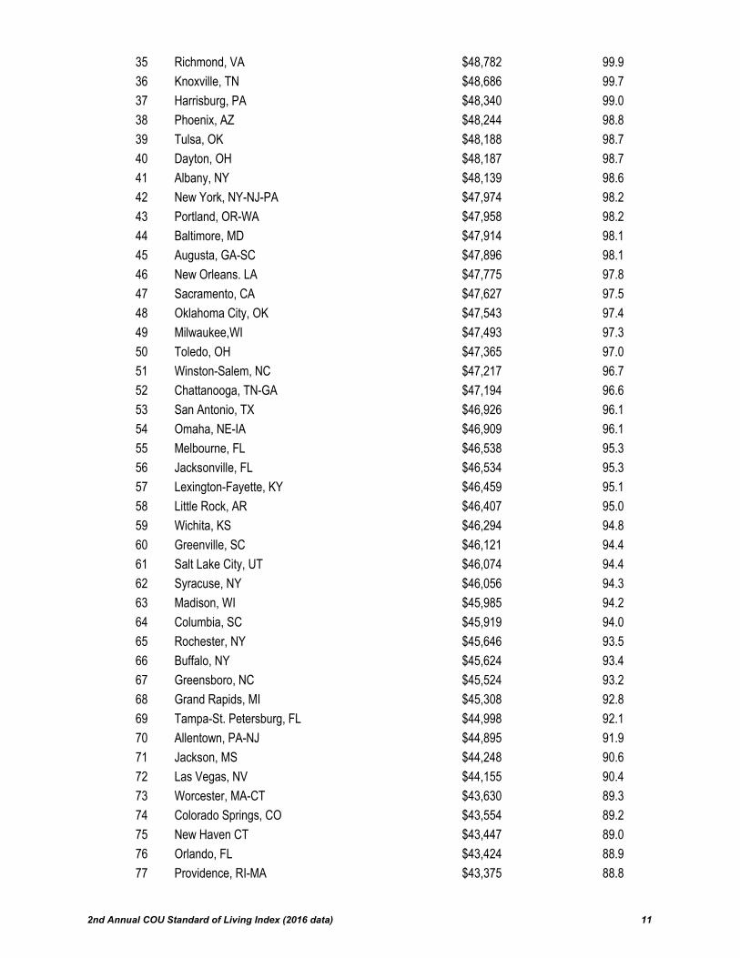
35 Richmond, VA $48,782 99.9

36 Knoxville, TN $48,686 99.7

37 Harrisburg, PA $48,340 99.0

38 Phoenix, AZ $48,244 98.8

39 Tulsa, OK $48,188 98.7

40 Dayton, OH $48,187 98.7

41 Albany, NY $48,139 98.6

42 New York, NY-NJ-PA $47,974 98.2

43 Portland, OR-WA $47,958 98.2

44 Baltimore, MD $47,914 98.1

45 Augusta, GA-SC $47,896 98.1

46 New Orleans. LA $47,775 97.8

47 Sacramento, CA $47,627 97.5

48 Oklahoma City, OK $47,543 97.4

49 Milwaukee,WI $47,493 97.3

50 Toledo, OH $47,365 97.0

51 Winston-Salem, NC $47,217 96.7

52 Chattanooga, TN-GA $47,194 96.6

53 San Antonio, TX $46,926 96.1

54 Omaha, NE-IA $46,909 96.1

55 Melbourne, FL $46,538 95.3

56 Jacksonville, FL $46,534 95.3

57 Lexington-Fayette, KY $46,459 95.1

58 Little Rock, AR $46,407 95.0

59 Wichita, KS $46,294 94.8

60 Greenville, SC $46,121 94.4

61 Salt Lake City, UT $46,074 94.4

62 Syracuse, NY $46,056 94.3

63 Madison, WI $45,985 94.2

64 Columbia, SC $45,919 94.0

65 Rochester, NY $45,646 93.5

66 Buffalo, NY $45,624 93.4

67 Greensboro, NC $45,524 93.2

68 Grand Rapids, MI $45,308 92.8

69 Tampa-St. Petersburg, FL $44,998 92.1

70 Allentown, PA-NJ $44,895 91.9

71 Jackson, MS $44,248 90.6

72 Las Vegas, NV $44,155 90.4

73 Worcester, MA-CT $43,630 89.3

74 Colorado Springs, CO $43,554 89.2

75 New Haven CT $43,447 89.0

76 Orlando, FL $43,424 88.9

77 Providence, RI-MA $43,375 88.8


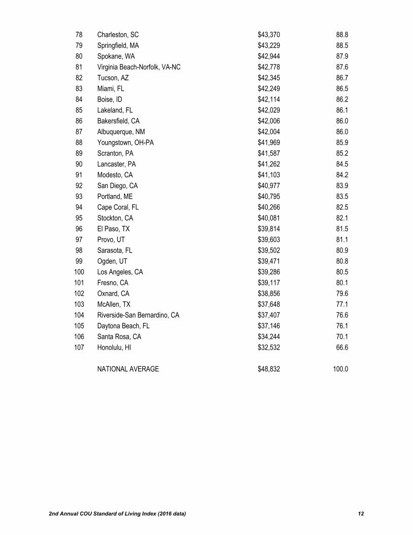
78 Charleston, SC $43,370 88.8

79 Springfield, MA $43,229 88.5

80 Spokane, WA $42,944 87.9

81 Virginia Beach-Norfolk, VA-NC $42,778 87.6

82 Tucson, AZ $42,345 86.7

83 Miami, FL $42,249 86.5

84 Boise, ID $42,114 86.2

85 Lakeland, FL $42,029 86.1

86 Bakersfield, CA $42,006 86.0

87 Albuquerque, NM $42,004 86.0

88 Youngstown, OH-PA $41,969 85.9

89 Scranton, PA $41,587 85.2

90 Lancaster, PA $41,262 84.5

91 Modesto, CA $41,103 84.2

92 San Diego, CA $40,977 83.9

93 Portland, ME $40,795 83.5

94 Cape Coral, FL $40,266 82.5

95 Stockton, CA $40,081 82.1

96 El Paso, TX $39,814 81.5

97 Provo, UT $39,603 81.1

98 Sarasota, FL $39,502 80.9

99 Ogden, UT $39,471 80.8

100 Los Angeles, CA $39,286 80.5

101 Fresno, CA $39,117 80.1

102 Oxnard, CA $38,856 79.6

103 McAllen, TX $37,648 77.1

104 Riverside-San Bernardino, CA $37,407 76.6

105 Daytona Beach, FL $37,146 76.1

106 Santa Rosa, CA $34,244 70.1

107 Honolulu, HI $32,532 66.6

NATIONAL AVERAGE $48,832 100.0


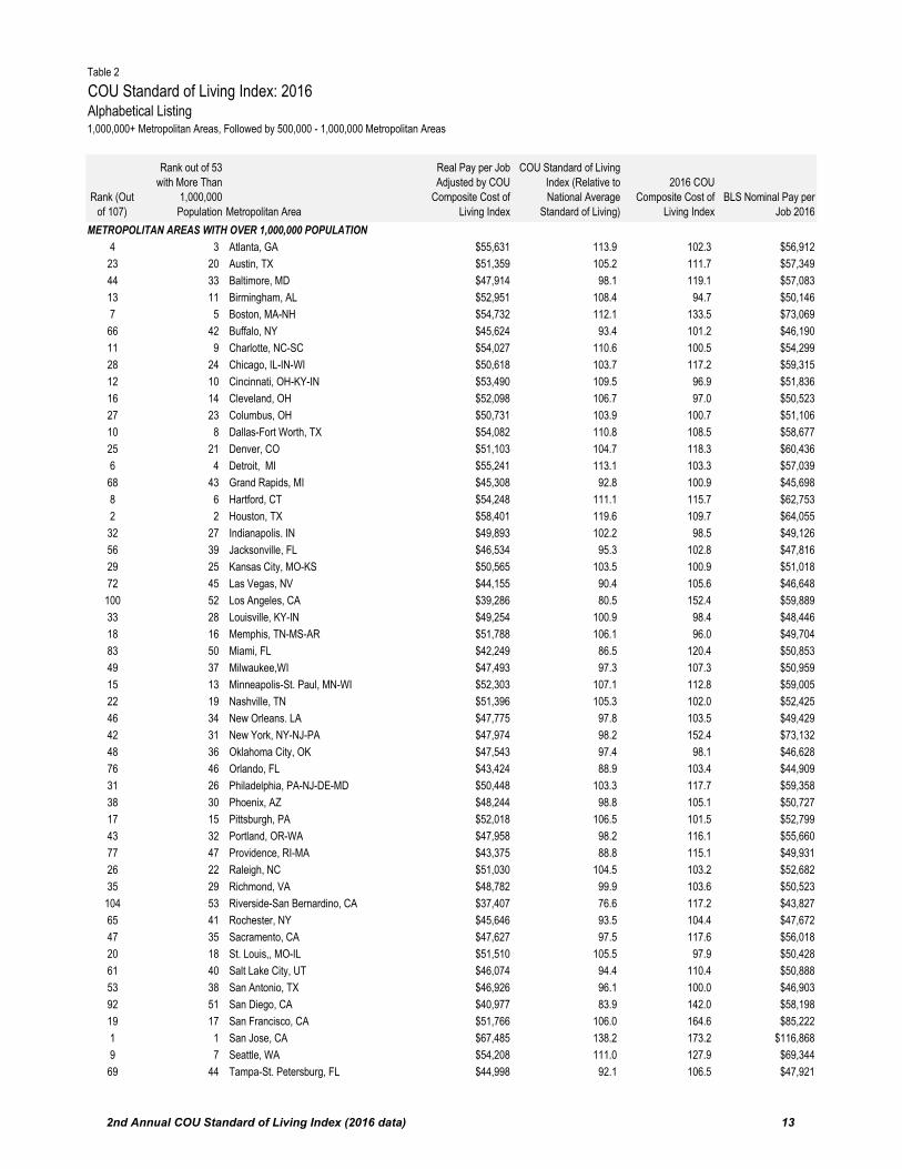
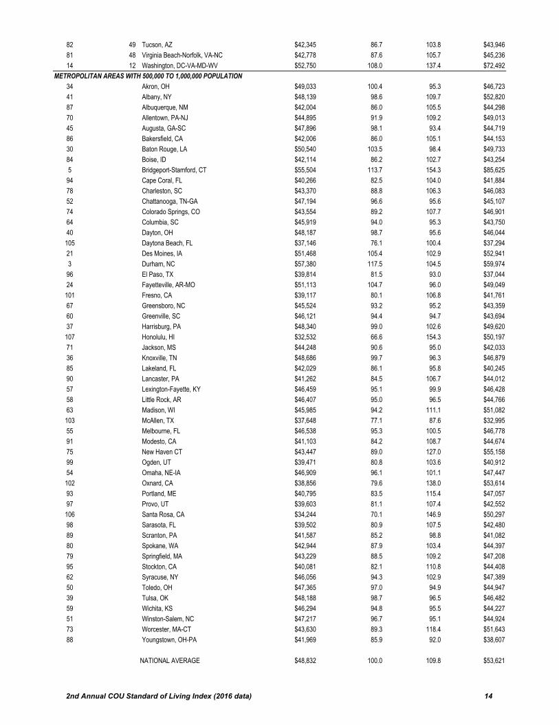
Table 2

COU Standard of Living Index: 2016Alphabetical Listing1,000,000+ Metropolitan Areas, Followed by 500,000 - 1,000,000 Metropolitan Areas

Rank (Out

of 107)

Rank out of 53

with More Than

1,000,000

Population Metropolitan Area

Real Pay per Job

Adjusted by COU

Composite Cost of

Living Index

COU Standard of Living

Index (Relative to

National Average

Standard of Living)

2016 COU

Composite Cost of

Living Index

BLS Nominal Pay per

Job 2016

METROPOLITAN AREAS WITH OVER 1,000,000 POPULATION

4 3 Atlanta, GA $55,631 113.9 102.3 $56,912

23 20 Austin, TX $51,359 105.2 111.7 $57,349

44 33 Baltimore, MD $47,914 98.1 119.1 $57,083

13 11 Birmingham, AL $52,951 108.4 94.7 $50,146

7 5 Boston, MA-NH $54,732 112.1 133.5 $73,069

66 42 Buffalo, NY $45,624 93.4 101.2 $46,190

11 9 Charlotte, NC-SC $54,027 110.6 100.5 $54,299

28 24 Chicago, IL-IN-WI $50,618 103.7 117.2 $59,315

12 10 Cincinnati, OH-KY-IN $53,490 109.5 96.9 $51,836

16 14 Cleveland, OH $52,098 106.7 97.0 $50,523

27 23 Columbus, OH $50,731 103.9 100.7 $51,106

10 8 Dallas-Fort Worth, TX $54,082 110.8 108.5 $58,677

25 21 Denver, CO $51,103 104.7 118.3 $60,436

6 4 Detroit, MI $55,241 113.1 103.3 $57,039

68 43 Grand Rapids, MI $45,308 92.8 100.9 $45,698

8 6 Hartford, CT $54,248 111.1 115.7 $62,753

2 2 Houston, TX $58,401 119.6 109.7 $64,055

32 27 Indianapolis. IN $49,893 102.2 98.5 $49,126

56 39 Jacksonville, FL $46,534 95.3 102.8 $47,816

29 25 Kansas City, MO-KS $50,565 103.5 100.9 $51,018

72 45 Las Vegas, NV $44,155 90.4 105.6 $46,648

100 52 Los Angeles, CA $39,286 80.5 152.4 $59,889

33 28 Louisville, KY-IN $49,254 100.9 98.4 $48,446

18 16 Memphis, TN-MS-AR $51,788 106.1 96.0 $49,704

83 50 Miami, FL $42,249 86.5 120.4 $50,853

49 37 Milwaukee,WI $47,493 97.3 107.3 $50,959

15 13 Minneapolis-St. Paul, MN-WI $52,303 107.1 112.8 $59,005

22 19 Nashville, TN $51,396 105.3 102.0 $52,425

46 34 New Orleans. LA $47,775 97.8 103.5 $49,429

42 31 New York, NY-NJ-PA $47,974 98.2 152.4 $73,132

48 36 Oklahoma City, OK $47,543 97.4 98.1 $46,628

76 46 Orlando, FL $43,424 88.9 103.4 $44,909

31 26 Philadelphia, PA-NJ-DE-MD $50,448 103.3 117.7 $59,358

38 30 Phoenix, AZ $48,244 98.8 105.1 $50,727

17 15 Pittsburgh, PA $52,018 106.5 101.5 $52,799

43 32 Portland, OR-WA $47,958 98.2 116.1 $55,660

77 47 Providence, RI-MA $43,375 88.8 115.1 $49,931

26 22 Raleigh, NC $51,030 104.5 103.2 $52,682

35 29 Richmond, VA $48,782 99.9 103.6 $50,523

104 53 Riverside-San Bernardino, CA $37,407 76.6 117.2 $43,827

65 41 Rochester, NY $45,646 93.5 104.4 $47,672

47 35 Sacramento, CA $47,627 97.5 117.6 $56,018

20 18 St. Louis,, MO-IL $51,510 105.5 97.9 $50,428

61 40 Salt Lake City, UT $46,074 94.4 110.4 $50,888

53 38 San Antonio, TX $46,926 96.1 100.0 $46,903

92 51 San Diego, CA $40,977 83.9 142.0 $58,198

19 17 San Francisco, CA $51,766 106.0 164.6 $85,222

1 1 San Jose, CA $67,485 138.2 173.2 $116,868

9 7 Seattle, WA $54,208 111.0 127.9 $69,344

69 44 Tampa-St. Petersburg, FL $44,998 92.1 106.5 $47,921


82 49 Tucson, AZ $42,345 86.7 103.8 $43,946

81 48 Virginia Beach-Norfolk, VA-NC $42,778 87.6 105.7 $45,236

14 12 Washington, DC-VA-MD-WV $52,750 108.0 137.4 $72,492

METROPOLITAN AREAS WITH 500,000 TO 1,000,000 POPULATION

34 Akron, OH $49,033 100.4 95.3 $46,723

41 Albany, NY $48,139 98.6 109.7 $52,820

87 Albuquerque, NM $42,004 86.0 105.5 $44,298

70 Allentown, PA-NJ $44,895 91.9 109.2 $49,013

45 Augusta, GA-SC $47,896 98.1 93.4 $44,719

86 Bakersfield, CA $42,006 86.0 105.1 $44,153

30 Baton Rouge, LA $50,540 103.5 98.4 $49,733

84 Boise, ID $42,114 86.2 102.7 $43,254

5 Bridgeport-Stamford, CT $55,504 113.7 154.3 $85,625

94 Cape Coral, FL $40,266 82.5 104.0 $41,884

78 Charleston, SC $43,370 88.8 106.3 $46,083

52 Chattanooga, TN-GA $47,194 96.6 95.6 $45,107

74 Colorado Springs, CO $43,554 89.2 107.7 $46,901

64 Columbia, SC $45,919 94.0 95.3 $43,750

40 Dayton, OH $48,187 98.7 95.6 $46,044

105 Daytona Beach, FL $37,146 76.1 100.4 $37,294

21 Des Moines, IA $51,468 105.4 102.9 $52,941

3 Durham, NC $57,380 117.5 104.5 $59,974

96 El Paso, TX $39,814 81.5 93.0 $37,044

24 Fayetteville, AR-MO $51,113 104.7 96.0 $49,049

101 Fresno, CA $39,117 80.1 106.8 $41,761

67 Greensboro, NC $45,524 93.2 95.2 $43,359

60 Greenville, SC $46,121 94.4 94.7 $43,694

37 Harrisburg, PA $48,340 99.0 102.6 $49,620

107 Honolulu, HI $32,532 66.6 154.3 $50,197

71 Jackson, MS $44,248 90.6 95.0 $42,033

36 Knoxville, TN $48,686 99.7 96.3 $46,879

85 Lakeland, FL $42,029 86.1 95.8 $40,245

90 Lancaster, PA $41,262 84.5 106.7 $44,012

57 Lexington-Fayette, KY $46,459 95.1 99.9 $46,428

58 Little Rock, AR $46,407 95.0 96.5 $44,766

63 Madison, WI $45,985 94.2 111.1 $51,082

103 McAllen, TX $37,648 77.1 87.6 $32,995

55 Melbourne, FL $46,538 95.3 100.5 $46,778

91 Modesto, CA $41,103 84.2 108.7 $44,674

75 New Haven CT $43,447 89.0 127.0 $55,158

99 Ogden, UT $39,471 80.8 103.6 $40,912

54 Omaha, NE-IA $46,909 96.1 101.1 $47,447

102 Oxnard, CA $38,856 79.6 138.0 $53,614

93 Portland, ME $40,795 83.5 115.4 $47,057

97 Provo, UT $39,603 81.1 107.4 $42,552

106 Santa Rosa, CA $34,244 70.1 146.9 $50,297

98 Sarasota, FL $39,502 80.9 107.5 $42,480

89 Scranton, PA $41,587 85.2 98.8 $41,082

80 Spokane, WA $42,944 87.9 103.4 $44,397

79 Springfield, MA $43,229 88.5 109.2 $47,208

95 Stockton, CA $40,081 82.1 110.8 $44,408

62 Syracuse, NY $46,056 94.3 102.9 $47,389

50 Toledo, OH $47,365 97.0 94.9 $44,947

39 Tulsa, OK $48,188 98.7 96.5 $46,482

59 Wichita, KS $46,294 94.8 95.5 $44,227

51 Winston-Salem, NC $47,217 96.7 95.1 $44,924

73 Worcester, MA-CT $43,630 89.3 118.4 $51,643

88 Youngstown, OH-PA $41,969 85.9 92.0 $38,607

NATIONAL AVERAGE $48,832 100.0 109.8 $53,621


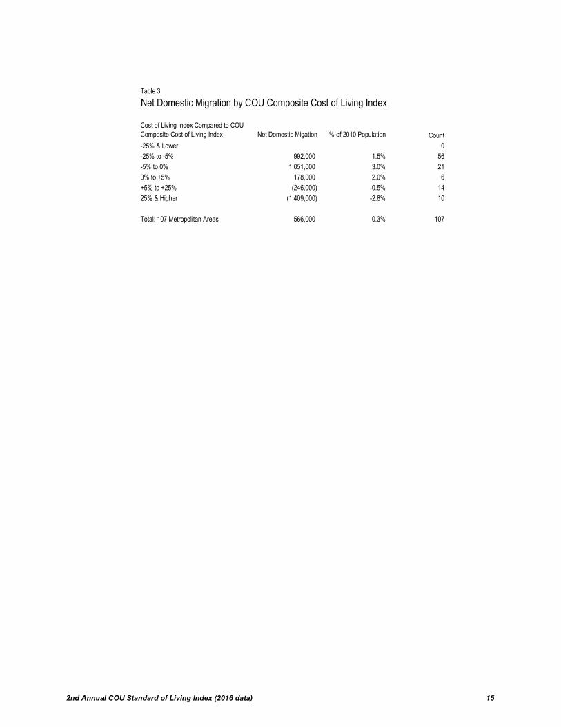
Table 3

Net Domestic Migration by COU Composite Cost of Living Index

Cost of Living Index Compared to COU

Composite Cost of Living Index Net Domestic Migation % of 2010 Population Count

-25% & Lower 0

-25% to -5% 992,000 1.5% 56

-5% to 0% 1,051,000 3.0% 21

0% to +5% 178,000 2.0% 6

+5% to +25% (246,000) -0.5% 14

25% & Higher (1,409,000) -2.8% 10

Total: 107 Metropolitan Areas 566,000 0.3% 107


2017 center for opportunity urbanism (cou) standard of ... · included. 2. the bea rpps, as...

Documents