2017 coastal master plan appendix c:...

Coastal Protection and Restoration Authority 150 Terrace Avenue, Baton Rouge, LA 70802 | [email protected] | www.coastal.la.gov

2017 Coastal Master Plan

Appendix C: Modeling Chapter 2 - Future Scenarios

Report: Final

Date: April 2017

Prepared By: The Water Institute of the Gulf

2017 Coastal Master Plan: Modeling

Page | ii

Coastal Protection and Restoration Authority

This document was prepared in support of the 2017 Coastal Master Plan being prepared by the

Coastal Protection and Restoration Authority (CPRA). CPRA was established by the Louisiana

Legislature in response to Hurricanes Katrina and Rita through Act 8 of the First Extraordinary

Session of 2005. Act 8 of the First Extraordinary Session of 2005 expanded the membership, duties,

and responsibilities of CPRA and charged the new authority to develop and implement a

comprehensive coastal protection plan, consisting of a master plan (revised every five years)

and annual plans. CPRA’s mandate is to develop, implement, and enforce a comprehensive

coastal protection and restoration master plan.

Suggested Citation:

Meselhe, E., White, E. D., and Reed, D. J., (2017). 2017 Coastal Master Plan: Appendix C:

Modeling Chapter 2 – Future Scenarios. Version Final. (p. 32). Baton Rouge, Louisiana: Coastal

Protection and Restoration Authority.


Page | iii

Acknowledgements

The authors would like to thank the RAND team (Jordan Fischbach, David Johnson, and Kenneth

Kuhn) for contributions from the CLARA storm analysis, the entire 2017 Coastal Master Plan

modeling team (listed in Chapter 1), the Predictive Models Technical Advisory Committee (PM-

TAC), external reviewers, and the Planning Tool team for their contributions to this effort. Thanks

also go to Jennifer Butler, Jeff Heaton, Marla Muse-Morris, and Mark Legendre for contractual

support and management, and to Taylor Kimball for editorial support. Lastly, the authors would

like to thank Natalie Peyronnin, Mark Leadon, and Ed Haywood for contributions during early

phases of the model improvement planning effort and Brian Harper for his contributions to early

phases of the PM-TAC.

This effort was funded by the Coastal Protection and Restoration Authority (CPRA) of Louisiana

under Cooperative Endeavor Agreement Number 2503-12-58, Task Order No. 03.


Page | iv

Executive Summary

Coastal Louisiana has experienced dramatic land loss since at least the 1930’s. A combination

of natural processes and human activities has resulted in the loss of over 1,880 square miles since

the 1930’s and a current land loss rate of 16.6 square miles per year. Not only has this land loss

resulted in increased environmental, economic, and social vulnerability, but these vulnerabilities

have been compounded by multiple disasters, including hurricanes, river floods, and the 2010

Deepwater Horizon oil spill, all of which have had a significant impact on the coastal

communities in Louisiana and other Gulf coast states. To address this crisis the 2007 Coastal

Master Plan was developed under the direction of the Louisiana Legislature. 2012 marked the

first five-year update to the plan, and the second update is scheduled for 2017.

A number of substantial revisions have been made in preparation for the 2017 Coastal Master

Plan modeling effort. Chapter 2 describes why environmental scenarios are needed for the 2017

Coastal Master Plan, and how the scenarios were developed. It also provides details on

selection of the environmental drivers, the plausible range of values for each driver, and the

analysis and modeling used to support the selection of values for each scenario.

Additional details for the modeling components are provided in a series of attachments.


Page | v

Table of Contents

Coastal Protection and Restoration Authority ............................................................................................ ii

List of Tables ....................................................................................................................................................... vi

List of Figures ...................................................................................................................................................... vi

List of Abbreviations ........................................................................................................................................ vii

Chapter 2: Future Scenarios ............................................................................................................................ 1

1.0 Introduction ............................................................................................................................................... 1 1.1 The Need for Scenarios ........................................................................................................................... 1 1.2 Developing Scenarios ............................................................................................................................. 2

2.0 Selection of Drivers and Identification of Ranges ............................................................................. 3 2.1 Revisiting the 2012 Coastal Master Plan .............................................................................................. 3 2.2 Why Fewer Drivers are considered for 2017........................................................................................ 5 2.3 Summary of Ranges for 2017 Drivers .................................................................................................... 5 2.4 Comparison of 2012 and 2017 Values ................................................................................................. 8

3.0 Analysis to Support Selection of Scenario Values.............................................................................. 9 3.1 Suggested Approaches for Value Selection ...................................................................................... 9 3.1.1 Option 1 – Baseline Comparison Multi-Phased Approach ......................................................... 10 3.1.2 Option 2 – Statistically Based Approach ........................................................................................ 10 3.2 Modeling to Identify Scenario Values ................................................................................................ 11 3.2.1 Sensitivity Analyses .............................................................................................................................. 12 3.2.2 Evaluation of Candidate Scenarios ................................................................................................ 19 3.2.3 Varying Storm Frequency and Intensity in CLARA ....................................................................... 20

4.0 Selection of Environmental Scenarios................................................................................................ 22

5.0 References .............................................................................................................................................. 23


Page | vi

List of Tables

Table 1: Overview of the Environmental Uncertainties (‘drivers’ in 2017 analyses) and Values used

to Define Two Future Scenarios for the 2012 Coastal Master Plan. ......................................................... 4

Table 2: 2017 Coastal Master Plan Environmental Driver Ranges, Compared to those Used in

2012. ..................................................................................................................................................................... 8

Table 3: Experimental Matrix Design of Environmental Drivers and Four Combinations. .................. 11

Table 4: List of the Sensitivity Runs Conducted to Assess Changes in Model Outputs of Land Area

in Association with Changing Environmental Drivers. .............................................................................. 12

Table 5: Values Used in the Five Candidate Environmental Scenarios. ............................................... 19

Table 6: EAD as a Function of Changes in Storminess. ............................................................................ 21

Table 7: EAD as a Function of Changes in Storminess - Coast wide Summary. .................................. 22

Table 8: Characteristics of the Environmental Scenarios to be used in the 2017 Coastal Master

Plan. ................................................................................................................................................................... 22

List of Figures

Figure 1: Comparison of Coast Wide Land Outputs for S20 (baseline) and S21 (baseline with mid

value for ESLR). ................................................................................................................................................. 13

Figure 2: Comparison of Coast Wide Land Outputs for Model Runs with Varying Subsidence and

Eustatic Sea Level Rise Rates.. ...................................................................................................................... 14

Figure 3: Comparison of Coast Wide Land Area for Model Runs with Varying Precipitation and

Evapotranspiration Rates............................................................................................................................... 15

Figure 4: Differences in Land Area between the Baseline Run (S20) and a Wetter Set of

Conditions (S33) for Selected Ecoregions. ................................................................................................. 16

Figure 5: Comparison of Coast Wide Land Area for Model Runs with Varying Storm Frequency

and Intensity. .................................................................................................................................................... 17

Figure 6: Differences in Land Area between the Baseline Run (S20) and an Increase in the

Number of Total Storms and the Frequency of Major Storms (S39) for Selected Ecoregions. ......... 18

Figure 7: Coast Wide Land Area under Future Without Action for the Five Candidate Scenarios

(see Table 7 for drivers included in each). ................................................................................................. 20


Page | vii

List of Abbreviations

ADCIRC Advanced Circulation

AVB Atchafalaya-Vermillion Bay

BRT Breton Sound

CAS Calcasieu

CLARA Coastal Louisiana Risk Assessment

CORS Continuously Operating Reference Stations

CPRA Coastal Protection And Restoration Authority

EAD Expected Annual Damage

ECHAM Max Planck Institute For Meteorology ECHAM5 General Circulation Model

ESLR Eustatic Sea Level Rise

FWOA Future Without Action

GCM General Circulation Model

GENMOM USGS and Portland State University GENMOM general circulation model

HSDRRS Hurricane and Storm Damage Risk Reduction System

HURDAT HURricane DATabases

ICM Integrated Compartment Model

LBA Lower Barataria

LO Less Optimistic

LPO Lower Pontchartrain

LTB Lower Terrebonne

MD Moderate

PDI Power Dissipation Index

PM-TAC Predictive Models Technical Advisory Committee


Page | viii

PR Plausible Range

UBA Upper Barataria

UPO Upper Pontchartrain

USACE U.S. Army Corp Of Engineers

UTB Upper Terrebonne


Page | 1

Chapter 2: Future Scenarios

1.0 Introduction

1.1 The Need for Scenarios

The objective of Louisiana’s Comprehensive Master Plan for a Sustainable Coast is to evaluate

and select restoration and protection projects that build and sustain the landscape and reduce

risk to communities from storm surge based flooding. Given the uncertainty associated with

future environmental conditions, models that seek to predict future outcomes must incorporate

some level of variability in their inputs to reflect such uncertainty. This is especially important to

help in decision making when planning long-term (50-year), large-scale (coast wide) restoration

and protection efforts for coastal Louisiana. There are many ways to consider unknown future

conditions, and selecting a strategy to incorporate those conditions into a modeling effort

depends on the types of information available and how the results will be used. Where there is

no known likelihood associated with environmental conditions but rather a range of plausible

future conditions, scenario analysis (e.g., Groves and Lempert, 2007; Mahmoud et al., 2009)

provides a viable way for decision makers to explore the effects of different possible future

conditions on the outcomes of interest. The primary role of scenarios in the master plan modeling

is to provide insight into project performance into the future, across a range of plausible future

conditions.

A scenario approach, evaluating model outcomes across different combinations of values for a

set of environmental drivers, was used in the development of the 2012 Coastal Master Plan. This

effort builds on the work conducted for the 2012 Coastal Master Plan and provides a foundation

for the selection of scenario values for the 2017 Coastal Master Plan. The resulting

representations of future environmental conditions captured in the scenarios are not intended to

represent “what will happen into the future;” instead, they are a means of gaining insight into

the uncertainty of the future and an acknowledgement that the past environmental conditions

will not necessarily repeat into the future. Including future scenarios in master plan analyses

allows for the consideration of a variety of plausible future conditions.

In preparation for the 2012 Coastal Master Plan, nine key environmental drivers were identified

for which it was challenging to determine a more or less likely set of values to drive the modeling

effort. Some of these environmental drivers are influenced by climate change or management

decisions in the future (e.g., eustatic sea level rise [ESLR] and river nutrient concentrations,

respectively), and some are based on processes that are not fully understood (e.g., subsidence,

marsh collapse threshold). Such complexity made it challenging to identify values for the future

scenarios to drive the models.

This report documents the procedures used to explore new data and literature regarding some

of the environmental drivers and develop a set of analyses to explore model output response to

different values for environmental drivers. These analyses are used to inform the selection of

environmental drivers and values to be used in scenarios for the 2017 Coastal Master Plan

modeling effort. Such analyses were not conducted prior to the selection of scenario values for

use in the 2012 Coastal Master Plan. Consequently, while the values were thought to each

contribute to change in model outputs, this hypothesis was not formally tested.


Page | 2

It is important to note that this report does not attempt to develop new science related to the

environmental drivers or their temporal/spatial patterns. There is also no attempt to develop new

forecasts or predictions of future conditions. Rather, this effort focuses on identifying the state of

the science and applying that knowledge for coastal planning purposes. As such, the work is

based on a combination of scientific literature, analysis of existing data, input from subject

matter experts, and best professional judgment where necessary.

1.2 Developing Scenarios

Scenarios for use in planning can be derived in a number of ways. In some cases, they are

developed by stakeholders and in others by using statistical methods to explore the possible

range of future circumstances once plausible ranges for individual drivers have been identified.

This report outlines options that were considered to explore model output response to changes

in environmental drivers and procedure used. All approaches had to be feasible given the time

and resource constraints of the planning process.

Once the nine key environmental drivers were identified for the 2012 Coastal Master Plan

analysis, documentation was assembled to describe the plausible range of each driver over the

50-year planning horizon (Table 3). In some cases, this documentation was based on a review of

the scientific literature. In other cases, ranges were generated using expert panels and/or

inspection of available historical data. Once a plausible range for each driver is established,

there are a number of ways scenario values can be selected. For 2012, expert opinion was used

to select values from within each of the ranges. These selected values were then combined into

a small set of future scenarios. One disadvantage of this approach is that while relatively simple

to explain to stakeholders (especially compared to some of the statistical approaches used by

others), the role of any individual driver in influencing model outcomes cannot be determined.

Stakeholders may assume all the drivers are equally important; this may or may not be the case.

Model outputs may be more sensitive to some environmental drivers than others. If that is the

case, scenario analyses could be focused on fewer drivers to enable decision makers to better

understand how future conditions influence master plan outcomes. A smaller number of drivers

in each scenario also reduces the complexity of communication with stakeholders.

The approaches described in this report involve testing the effects of different values selected

from the plausible ranges of several environmental drivers on key model outputs. The results of

the model runs can then be explored to show which values across the plausible range of the

environmental drivers produce change in model outputs. This information can then be used to

inform the selection of a small set of scenario values for use in the 2017 Coastal Master Plan and

makes it more likely that the different scenarios will produce a change in master plan model

outputs. Not only do the experimental analyses described below facilitate the development of

the future scenarios, they also provide valuable insight into overall model sensitivity which can

be highly important when interpreting model outputs.

Due to limited time and resources, the experimental analyses described herein to identify

scenario values were not applied to the surge and wave modeling component (incorporated

using ADCIRC (Advanced CIRCulation Model)), but the surge and wave analyses are responsive

to the values chosen for environmental drivers. Future storm surge and wave conditions will be

predicted based on landscape conditions where landscape change will be driven by different

values of environmental driver associated with each scenario. Some testing of candidate

scenario values for storm intensity and frequency in the Coastal Louisiana Risk Assessment

(CLARA) model was conducted prior to finalizing the values for the environmental scenarios.

Further discussion of scenario values to be used in the risk analysis (e.g., fragility, population

growth) can be found in Attachment C3-25.


Page | 3

There are four primary steps in developing scenarios for use in the 2017 Coastal Master Plan:

1. Revisit the 2012 Coastal Master Plan work on future scenarios select drivers that are

relevant to the 2017 analyses, and identify whether plausible ranges for the relevant

environmental drivers should be modified, using recent literature, data, and other

information;

2. Assess the response of key model outputs to changes in value of the environmental

drivers

a. Design focused numerical experiments and perform analysis to assess the

response of key outputs of the 2017 Coastal Master Plan Integrated

Compartment Model (ICM)

b. Sensitivity testing, using 2012 data, with CLARA to ensure that variation in storm

frequency and intensity would influence the performance of risk reduction

projects;

3. Conduct ICM model runs on a range of candidate scenario values to confirm outputs

based on combinations of driver values; and

4. Identify three scenarios (combination of values of environmental drivers) to be used in

the 2017 Coastal Master Plan modeling effort.

Because scientific understanding of environmental conditions continues to grow and evolve, fall

2014 (time this report was written) was used as the ‘stopping point’ for new information to be

included/considered in the identification of plausible ranges, as time is needed for the technical

team to implement the experimental model runs and design the scenarios that will be used in

the 2017 Coastal Master Plan modeling. New information and data made available after fall

2014 will be included in future master plan updates.

2.0 Selection of Drivers and Identification of Ranges

2.1 Revisiting the 2012 Coastal Master Plan

Nine key environmental drivers considered to have uncertain outcomes over the next 50 years

were used to develop future scenarios for the 2012 Coastal Master Plan technical analysis.

Appendix C: Environmental Scenarios (CPRA, 2012) provides an overview of each of the

environmental drivers included, plausible ranges for those drivers across a 50-year planning

horizon, and a rationale for selecting values from within those ranges to formulate the future

scenarios. Table 3 provides an overview of the drivers, plausible ranges considered, and the

values used to define two future scenarios – ‘moderate’ and ‘less optimistic’ – for the 2012

Coastal Master Plan. A third scenario was also incorporated in the final 2012 analysis; this

scenario was identical to the ‘moderate’ scenario but had a eustatic sea level rise (ESLR) value

of 0.78 m over 50 years.


Page | 4

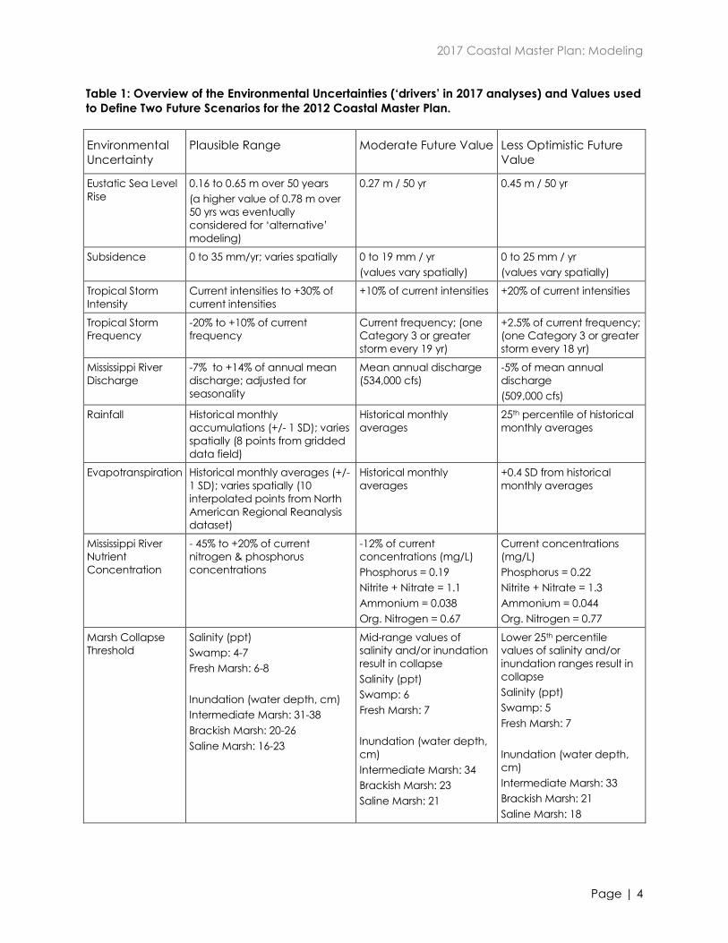
Table 1: Overview of the Environmental Uncertainties (‘drivers’ in 2017 analyses) and Values used

to Define Two Future Scenarios for the 2012 Coastal Master Plan.

Environmental

Uncertainty

Plausible Range Moderate Future Value Less Optimistic Future

Value

Eustatic Sea Level

Rise

0.16 to 0.65 m over 50 years

(a higher value of 0.78 m over

50 yrs was eventually

considered for ‘alternative’

modeling)

0.27 m / 50 yr 0.45 m / 50 yr

Subsidence 0 to 35 mm/yr; varies spatially

0 to 19 mm / yr

(values vary spatially)

0 to 25 mm / yr

(values vary spatially)

Tropical Storm

Intensity

Current intensities to +30% of

current intensities

+10% of current intensities +20% of current intensities

Tropical Storm

Frequency

-20% to +10% of current

frequency

Current frequency; (one

Category 3 or greater

storm every 19 yr)

+2.5% of current frequency;

(one Category 3 or greater

storm every 18 yr)

Mississippi River

Discharge

-7% to +14% of annual mean

discharge; adjusted for

seasonality

Mean annual discharge

(534,000 cfs)

-5% of mean annual

discharge

(509,000 cfs)

Rainfall Historical monthly

accumulations (+/- 1 SD); varies

spatially (8 points from gridded

data field)

Historical monthly

averages

25th percentile of historical

monthly averages

Evapotranspiration Historical monthly averages (+/-

1 SD); varies spatially (10

interpolated points from North

American Regional Reanalysis

dataset)

Historical monthly

averages

+0.4 SD from historical

monthly averages

Mississippi River

Nutrient

Concentration

- 45% to +20% of current

nitrogen & phosphorus

concentrations

-12% of current

concentrations (mg/L)

Phosphorus = 0.19

Nitrite + Nitrate = 1.1

Ammonium = 0.038

Org. Nitrogen = 0.67

Current concentrations

(mg/L)

Phosphorus = 0.22

Nitrite + Nitrate = 1.3

Ammonium = 0.044

Org. Nitrogen = 0.77

Marsh Collapse

Threshold

Salinity (ppt)

Swamp: 4-7

Fresh Marsh: 6-8

Inundation (water depth, cm)

Intermediate Marsh: 31-38

Brackish Marsh: 20-26

Saline Marsh: 16-23

Mid-range values of

salinity and/or inundation

result in collapse

Salinity (ppt)

Swamp: 6

Fresh Marsh: 7

Inundation (water depth,

cm)

Intermediate Marsh: 34

Brackish Marsh: 23

Saline Marsh: 21

Lower 25th percentile

values of salinity and/or

inundation ranges result in

collapse

Salinity (ppt)

Swamp: 5

Fresh Marsh: 7

Inundation (water depth,

cm)

Intermediate Marsh: 33

Brackish Marsh: 21

Saline Marsh: 18


Page | 5

2.2 Why Fewer Drivers are considered for 2017

Early in the model improvement work for the 2017 Coastal Master Plan, model team leaders

were asked to identify the most important drivers that should be considered in the scenario

analysis. Their recommendation was to begin with the same drivers used in 2012 with the

exception of the marsh collapse threshold; it is proposed to explore the influence of uncertainty

in this environmental driver during the planned model uncertainty analysis. This is recommended

because marsh collapse threshold is not an uncertainty in terms of unknown future

environmental conditions; rather, it is an uncertainty of our understanding of the current

conditions and processes at work.

A literature and data review was conducted to update the plausible range of each remaining

driver by incorporating the latest available information. The list of drivers was later reconsidered,

as the ICM began to take shape, in terms of each driver’s likely impact on model outcomes.

Removing non-critical drivers from the scenario analysis results in a more robust experimental

design for testing model response to the remaining environmental drivers – those drivers likely to

have a more substantial impact on model outputs. It also reduced the time and resources

needed to complete the analysis.

The following is an explanation of the changes made to the list of drivers for 2017 compared to

2012; changes to the ranges are provided in Table 4:

Mississippi River Discharge – this is being removed from the 2017 future scenarios analysis.

Based on the literature review conducted, including a review of the literature that was

used to identify the range used in the 2012 effort, the recommendation is to remove

Mississippi River discharge from the scenario analysis, as there is little evidence to support

a change in discharge in the future, and instead use the historical hydrograph without

adjustments.

Precipitation – this is a change in terminology from Rainfall in the 2012 effort to indicate

inclusion of all forms of precipitation.

Mississippi River Nutrient Concentration – this is being removed from the 2017 future

scenarios analysis. The 2017 Coastal Master Plan will model nutrients in the water quality

subroutine and with a nitrogen uptake subroutine; however, model outputs that depend

on these water quality calculations are not expected to be primary decision drivers in

planning efforts. Therefore, future uncertainty of nutrient concentrations is unlikely to alter

planning decisions made for the 2017 Coastal Master Plan; this driver will no longer vary

across future scenarios.

2.3 Summary of Ranges for 2017 Drivers

This section provides an overview of each environmental driver that is included in the 2017

Coastal Master Plan future scenarios analysis. Overviews include a brief statement regarding the

values used in the 2012 Coastal Master Plan and the rationale for setting the plausible 50-year

ranges (2015 – 2065) for use in the 2017 Coastal Master Plan. Table 4 compares the 2017 ranges

to those used in 2012, including the values used in the 2012 moderate and less optimistic

scenarios. Additional details on each of the drivers are provided in Attachments C2-1- C2-4.


Page | 6

Eustatic Sea Level Rise (ESLR)

The 2012 plausible range for ESLR was established on the basis of a data and literature review.

The low end of the range assumed no acceleration of the current rate beyond a recent

observed linear rate, and the high end of the range assumed acceleration consistent with the

National Research Council (NRC, 1987) scenario used to define the high sea level rise scenario

for the U.S. Army Corps of Engineers Circular #1165-2-211 (USACE, 2009). For the final 2012

analysis, a ‘very high’ ESLR rate was incorporated, based on Vermeer and Rahmstorf (2009).

Although the full breadth of historical work on this topic was considered for updating the 2017

range, emphasis was placed on new observations and predictive modeling generated

between the 2010 completion of the review that informed the 2012 Coastal Master Plan models

and fall 2014. Specifically, input for setting the new range included altimetry data, western

Florida tide gauge stations, an updated U.S. Army Corps of Engineers Circular #1165-2-212

(USACE, 2011), National Research Council 2012 sea level rise estimates and regional

modifications (NRC, 2012), as well as a set of sea level rise scenarios and regional modifications

included in the 2013 5th Assessment Report of the Intergovernmental Panel on Climate Change.

To establish the full plausible range of future sea level rise, this review equally evaluated results

from both process-based and semi-empirical predictive models. The result is a slightly wider

plausible range of values compared to 2012.

Note: only eustatic (global) or regional sea level rise rates were used, as the subsidence

component of locally specific relative sea level rise is accounted for separately in the 2017

modeling effort.

For more information on eustatic sea level rise, see Attachment C2-1.

Subsidence

Subsidence, as applied in the 2012 Coastal Master Plan scenarios was derived from a map of

plausible subsidence rates (ranging from 0 to 35 mm yr-1) across coastal Louisiana that were

differentiated into 17 geographical regions. Recent technical literature, information, and data

were identified and reviewed to determine if the accuracy and spatial variability of the 2012

subsidence rates or spatial coverage could be improved. No new definitive studies on

subsidence were found to provide coast wide predictions of future rates, and there are issues of

concern with the two new data sources considered. For example, the tide gauge data analysis

likely better reflects relative sea level rise not enabling the specific identification of subsidence,

and the Continuously Operating Reference Stations (CORS) data are largely derived from

instrumentation mounted on buildings which may not reflect the open estuary rates.

Considering the lack of definitive data or new studies on which to justify modifying the spatial

polygon boundaries, the recommendation is for the 2017 Coastal Master Plan to use the same

geographic regions and subsidence rates therein as the 2012 Coastal Master Plan.

For more information on subsidence, see Attachment C2-2.

Precipitation

In the 2012 Coastal Master Plan modeling effort, the plausible range of precipitation (referred to

in 2012 as Rainfall) was based on historical monthly accumulations (+/- 1 SD) using records from

1990-2010. Eight precipitation gauges were used to provide the spatial variability of the rainfall

pattern across the Louisiana coast.


Page | 7

However, general circulation models (GCMs) are now available and provide information on the

impact of greenhouse gas emissions on future climate and are increasingly used to develop

regional models of future climate. The availability of both these GCM and regional climate

datasets have resulted in the recent incorporation of climate projections in numerous large-

scale water resource planning efforts (Hagemann et al., 2012; Huntington et al., 2014; Sankovich

et al., 2013).

Three regional climate projections (developed from GFDL, ECHAM, and GENMOM GCM climate

projections and dynamically downscaled via the RegCM3 regional climate model; Hostetler et

al., 2011) were used to determine a range of future precipitation conditions across coastal

Louisiana for use in the 2017 Coastal Master Plan. In addition to these three future projections of

climate, historic records of precipitation were considered when developing the plausible range.

The low end of the 2017 precipitation range is set by GENMOM data and represents an

approximate 5% decrease in 50-year cumulative precipitation compared to historical data. The

high end of the range is set by the ECHAM data and represents an approximate 14% increase in

50-year cumulative precipitation compared to historical data.

For more information on precipitation, see Attachment C2-3.

Evapotranspiration

In the 2012 Coastal Master Plan modeling effort, the plausible range of evapotranspiration was

based on historical (calculated via Penman-Monteith) monthly accumulations (+/- 1 SD). These

monthly values did not vary temporally (e.g., all 50 January evapotranspiration values were the

same for each simulated year); however, the data varied spatially across the coast per 10 points

extracted from existing datasets derived from climatic data.

The same three regional climate projections used to develop precipitation scenarios (as

discussed in the previous section of this report) were also used to determine a range of future

evapotranspiration conditions across coastal Louisiana. In addition to these future projections of

climate, the historic monthly mean potential evapotranspiration rates (calculated via Penman-

Monteith) were considered in developing the plausible range. The low end of the 2017

evapotranspiration range is set by GENMOM data and represents a 30% decrease in 50-year

cumulative evapotranspiration compared to historical (Penman-Monteith). The high end of the

ranges is set by the Penman-Monteith data and represents historic monthly mean potential

evapotranspiration.

For more information on precipitation, see Attachment C2-3.

Tropical Storm Intensity

In 2012, the plausible range tropical storm intensity was based on a suite of literature, including

global and regional models and expert input from the 2012 Coastal Master Plan risk assessment

modeling team.

Future hurricane intensity was revisited for the 2017 effort and the revised plausible range of

future change builds off an updated literature review with expert input from the risk assessment

modeling team. The range was drawn from several robust modeling efforts that projected

potential changes in tropical storm intensity using central pressure deficit, wind speed, and

power dissipation index (PDI). Recommended plausible ranges are based on projections of

Atlantic Ocean Basin changes only, although studies analyzing potential changes in the Pacific

and global basins have been noted. Both the literature reviewed and the historical record (since

1980) provide evidence to suggest an increasing trend in tropical storm intensity; therefore an


Page | 8

increase in overall intensity compared to existing conditions is suggested for the 50-year period

of analysis.

Note: due to the nature of the storms in the synthetic storm suite being used for the 2017 Coastal

Master Plan modeling effort, there are limitations in the possible adjustments of storm intensity for

the landscape analyses. Therefore tropical storm intensity will not be included in the ICM future

scenarios; rather, it will be reserved for use in the risk assessment modeling (ADCIRC and CLARA).

For more information on tropical storm intensity, see Attachment C2-4.

Tropical Storm Frequency

In 2012, the plausible range of tropical storm frequency was based on a suite of literature,

including global and regional models and expert input from the 2012 Coastal Master Plan risk

assessment modeling team. During this effort, only the frequency of Category 3 hurricanes or

higher was considered.

Based on a literature review including projections of recent modeling efforts and expert input

from the risk assessment modeling team, several adjustments are suggested. The 2017 Coastal

Master Plan will consider all tropical storms and major hurricanes separately, with a decrease in

the frequency of all tropical storms and an increase in major hurricanes. Specifically, the 2017

revision proposes a slight reduction in the frequency of all tropical storms compared to what was

used in the 2012 Coastal Master Plan but a higher frequency of major hurricanes.

Recommended plausible ranges are based on projections of Atlantic Ocean Basin changes

only, although studies analyzing potential changes in the Pacific and global basins have been

noted.

For more information on tropical storm frequency, see Attachment C2-4.

2.4 Comparison of 2012 and 2017 Values

For ease of comparison, Table 4 provides a summary of the 2012 Coastal Master Plan plausible

range and moderate and less optimistic scenario values as well as the plausible range proposed

for the 2017 effort.

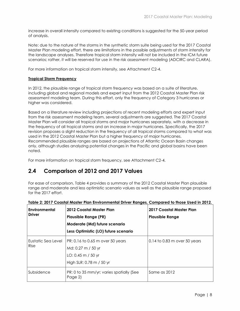
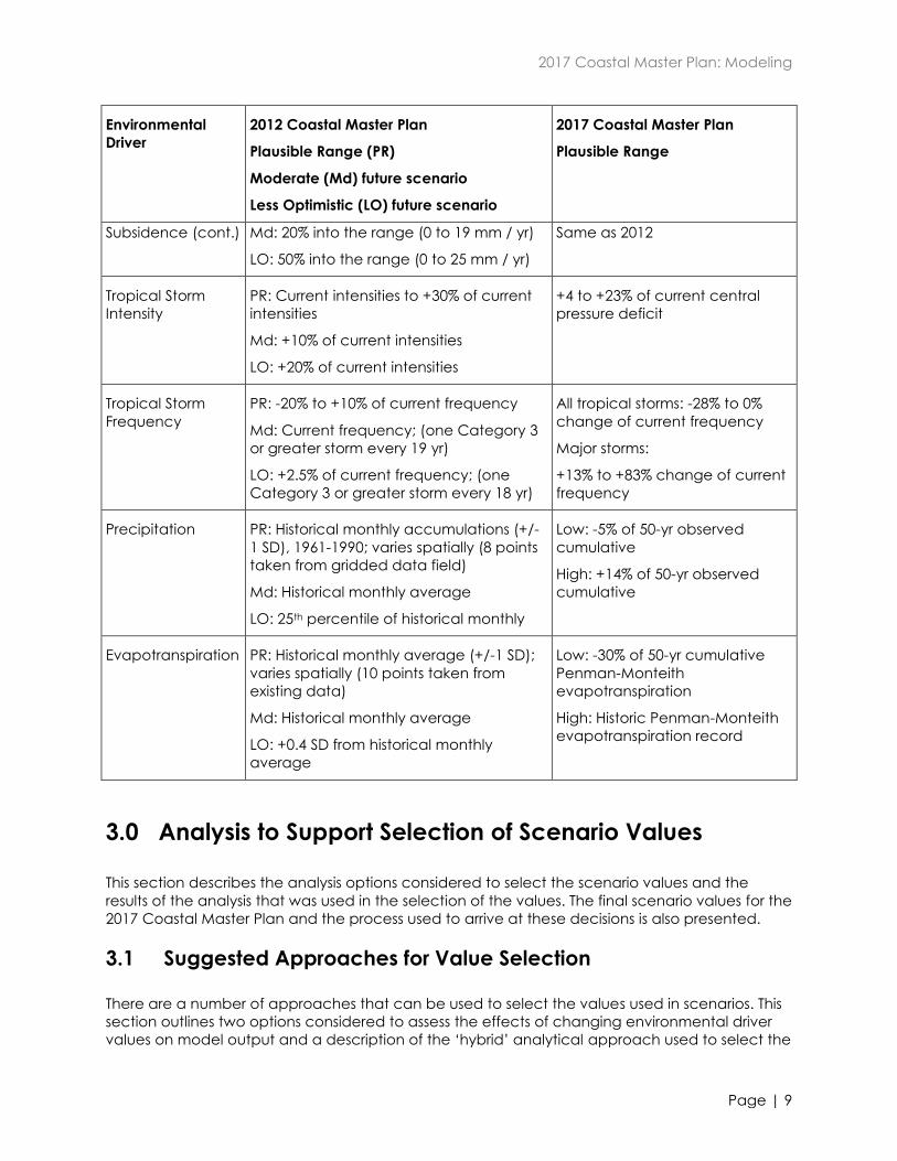
Table 2: 2017 Coastal Master Plan Environmental Driver Ranges, Compared to those Used in 2012.

Environmental

Driver


Plausible Range (PR)

Moderate (Md) future scenario

Less Optimistic (LO) future scenario


Plausible Range

Eustatic Sea Level

Rise

PR: 0.16 to 0.65 m over 50 years

Md: 0.27 m / 50 yr

LO: 0.45 m / 50 yr

High SLR: 0.78 m / 50 yr

0.14 to 0.83 m over 50 years

Subsidence PR: 0 to 35 mm/yr; varies spatially (See

Page 2)

Same as 2012


Page | 9

Environmental

Driver


Plausible Range (PR)

Moderate (Md) future scenario

Less Optimistic (LO) future scenario


Plausible Range

Subsidence (cont.) Md: 20% into the range (0 to 19 mm / yr)

LO: 50% into the range (0 to 25 mm / yr)

Same as 2012

Tropical Storm

Intensity

PR: Current intensities to +30% of current

intensities

Md: +10% of current intensities

LO: +20% of current intensities

+4 to +23% of current central

pressure deficit

Tropical Storm

Frequency

PR: -20% to +10% of current frequency

Md: Current frequency; (one Category 3

or greater storm every 19 yr)

LO: +2.5% of current frequency; (one

Category 3 or greater storm every 18 yr)

All tropical storms: -28% to 0%

change of current frequency

Major storms:

+13% to +83% change of current

frequency

Precipitation PR: Historical monthly accumulations (+/-

1 SD), 1961-1990; varies spatially (8 points

taken from gridded data field)

Md: Historical monthly average

LO: 25th percentile of historical monthly

Low: -5% of 50-yr observed

cumulative

High: +14% of 50-yr observed

cumulative

Evapotranspiration PR: Historical monthly average (+/-1 SD);

varies spatially (10 points taken from

existing data)

Md: Historical monthly average

LO: +0.4 SD from historical monthly

average

Low: -30% of 50-yr cumulative

Penman-Monteith

evapotranspiration

High: Historic Penman-Monteith

evapotranspiration record

3.0 Analysis to Support Selection of Scenario Values

This section describes the analysis options considered to select the scenario values and the

results of the analysis that was used in the selection of the values. The final scenario values for the

2017 Coastal Master Plan and the process used to arrive at these decisions is also presented.

3.1 Suggested Approaches for Value Selection

There are a number of approaches that can be used to select the values used in scenarios. This

section outlines two options considered to assess the effects of changing environmental driver

values on model output and a description of the ‘hybrid’ analytical approach used to select the


Page | 10

values for scenarios for the 2017 Coastal Master Plan. Land area is a primary decision driver for

the 2017 Coastal Master Plan; these options were developed for consideration of the effect of

scenario values on coast wide land. The effect of changing storm intensity and frequency on

CLARA damage estimates is assessed separately (section 3.2.3).

3.1.1 Option 1 – Baseline Comparison Multi-Phased Approach

This approach is grounded in having a ‘baseline’ model run intended to represent historical or

moderate conditions for comparison to previous outputs or other known conditions. Additional

model runs with specific changes to environmental drivers can be performed and compared to

the baseline simulation. The intent of this comparison is to determine the effects of change in

individual environmental drivers as well as several interactive driver combinations on model

outcomes. The first phase of simulations indicates the changes to specific environmental drivers;

all other drivers would assume the same values used in the baseline model run. Later phases

would change combinations of drivers based on the findings from the first phase and

understanding of how environmental factors interact to influence coastal change.

The phased approach provides flexibility to design simulations to examine specific spatial

considerations (e.g., some drivers may be expected to have a greater effect on certain regions

of the coast), while other simulations would focus on temporal considerations (e.g., some drivers

require a full 50-year model run to assess the full breadth of their impacts, but others may not).

In addition, testing drivers individually and collectively in different phases allows environmental

drivers that do not show strong influence on the model outputs across their range in the first

phase of runs to be eliminated unless there is a reasonable hypotheses that they may have more

influence when interacting with a non-baseline value of another driver. A second phase of the

analysis could consider values between those used in the first phase and/or could consider

hypothesized interactions among changes in drivers (e.g., the effect of changing

precipitation/evapotranspiration when SLR is at its highest). The phased approach would allow

for testing of key questions or concerns that may arise from the first phase of model simulations in

a subsequent phase of simulations.

An example design of the first phase of analysis for this approach is provided in Attachment C2-

5: Options for Sensitivity Analyses Table 1. Reference to “moderate” and “less optimistic” refers to

the 2012 Coastal Master Plan scenario values.

3.1.2 Option 2 – Statistically Based Approach

This option includes a matrix of targeted model runs to examine the combined impact of

changes in the environmental drivers on the model output as well as to explore the interaction

among the environmental drivers. In option 2, the key environmental drivers are organized into

three groups. The 64 runs represent each possible mixture of the four combinations for each

grouping of drivers (i.e., 4 combinations ^ 3 driver groups = 64), and the intent would be to

perform all simulations in a single phase (Table 5). The full set of model runs are listed in

Attachment C2-5: Options for Sensitivity Analyses Table 2. In some cases, the combinations

enable exploration of drivers within a group and in other cases spatial variation in outputs may

be used to tease out the effects, for instance, of subsidence (which varies spatially) from ESLR

(which is a single value coast wide) for each combination. In comparison to option 1, this

approach is faster because it does not require iterations. However, it can only explore a specific

set of values that must be defined before the analysis begins. Given this, it may be difficult to

determine scenario values for each driver since only three values for each driver will be included


Page | 11

in the analysis given the limited time available for the analysis. As such, decisions for selecting

values for inclusion in the three future scenarios would be drawn from insights gained from these

64 model runs.

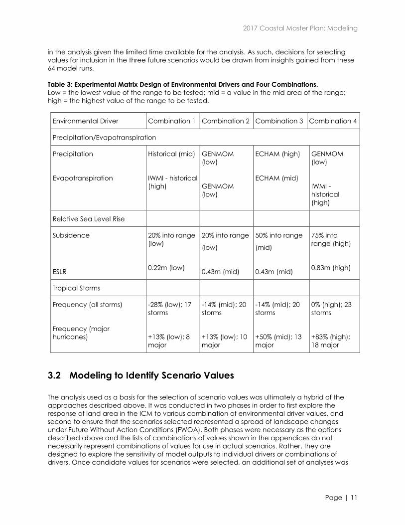
Table 3: Experimental Matrix Design of Environmental Drivers and Four Combinations.

Low = the lowest value of the range to be tested; mid = a value in the mid area of the range;

high = the highest value of the range to be tested.

Environmental Driver Combination 1 Combination 2 Combination 3 Combination 4

Precipitation/Evapotranspiration

Precipitation

Evapotranspiration

Historical (mid)

IWMI - historical

(high)

GENMOM

(low)

GENMOM

(low)

ECHAM (high)

ECHAM (mid)

GENMOM

(low)

IWMI -

historical

(high)

Relative Sea Level Rise

Subsidence

ESLR

20% into range

(low)

0.22m (low)

20% into range

(low)

0.43m (mid)

50% into range

(mid)

0.43m (mid)

75% into

range (high)

0.83m (high)

Tropical Storms

Frequency (all storms)

Frequency (major

hurricanes)

-28% (low); 17

storms

+13% (low); 8

major

-14% (mid); 20

storms

+13% (low); 10

major

-14% (mid); 20

storms

+50% (mid); 13

major

0% (high); 23

storms

+83% (high);

18 major

3.2 Modeling to Identify Scenario Values

The analysis used as a basis for the selection of scenario values was ultimately a hybrid of the

approaches described above. It was conducted in two phases in order to first explore the

response of land area in the ICM to various combination of environmental driver values, and

second to ensure that the scenarios selected represented a spread of landscape changes

under Future Without Action Conditions (FWOA). Both phases were necessary as the options

described above and the lists of combinations of values shown in the appendices do not

necessarily represent combinations of values for use in actual scenarios. Rather, they are

designed to explore the sensitivity of model outputs to individual drivers or combinations of

drivers. Once candidate values for scenarios were selected, an additional set of analyses was


Page | 12

conducted to explore trends over time and to support the selection of three sets of scenario

values to move forward.

3.2.1 Sensitivity Analyses

Table 4 shows the values tested with model runs. Run S20 is the ‘baseline’ model run intended to

represent historical conditions. The number of model runs and the values tested were identified

based on the time and resources available to conduct the analysis, professional judgment of

the potential role of different drivers, and the need to test sensitivity to changes in storm intensity

and frequency given that these factors did not influence landscape change in the 2012 Coastal

Master Plan modeling.

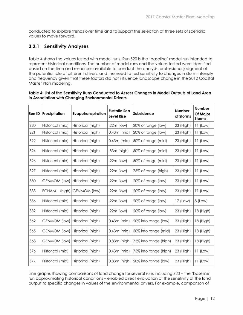
Table 4: List of the Sensitivity Runs Conducted to Assess Changes in Model Outputs of Land Area

in Association with Changing Environmental Drivers.

Run ID Precipitation Evapotranspiration Eustatic Sea

Level Rise Subsidence

Number

of Storms

Number

Of Major

Storms

S20 Historical (mid) Historical (high) .22m (low) 20% of range (low) 23 (High) 11 (Low)

S21 Historical (mid) Historical (high) 0.43m (mid) 20% of range (low) 23 (High) 11 (Low)

S22 Historical (mid) Historical (high) 0.43m (mid) 50% of range (mid) 23 (High) 11 (Low)

S24 Historical (mid) Historical (high) .83m (high) 50% of range (mid) 23 (High) 11 (Low)

S26 Historical (mid) Historical (high) .22m (low) 50% of range (mid) 23 (High) 11 (Low)

S27 Historical (mid) Historical (high) .22m (low) 75% of range (high) 23 (High) 11 (Low)

S30 GENMOM (low) Historical (high) .22m (low) 20% of range (low) 23 (High) 11 (Low)

S33 ECHAM (high) GENMOM (low) .22m (low) 20% of range (low) 23 (High) 11 (Low)

S36 Historical (mid) Historical (high) .22m (low) 20% of range (low) 17 (Low) 8 (Low)

S39 Historical (mid) Historical (high) .22m (low) 20% of range (low) 23 (High) 18 (High)

S62 GENMOM (low) Historical (high) 0.43m (mid) 20% into range (low) 23 (High) 18 (High)

S65 GENMOM (low) Historical (high) 0.43m (mid) 50% into range (mid) 23 (High) 18 (High)

S68 GENMOM (low) Historical (high) 0.83m (high) 75% into range (high) 23 (High) 18 (High)

S76 Historical (mid) Historical (high) 0.43m (mid) 75% into range (high) 23 (High) 11 (Low)

S77 Historical (mid) Historical (high) 0.83m (high) 20% into range (low) 23 (High) 11 (Low)

Line graphs showing comparisons of land change for several runs including S20 – the ‘baseline’

run approximating historical conditions – enabled direct evaluation of the sensitivity of the land

output to specific changes in values of the environmental drivers. For example, comparison of


Page | 13

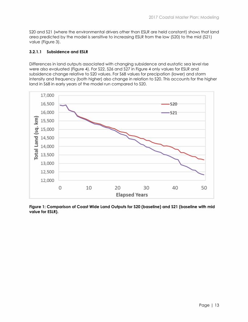
S20 and S21 (where the environmental drivers other than ESLR are held constant) shows that land

area predicted by the model is sensitive to increasing ESLR from the low (S20) to the mid (S21)

value (Figure 3).

3.2.1.1 Subsidence and ESLR

Differences in land outputs associated with changing subsidence and eustatic sea level rise

were also evaluated (Figure 4). For S22, S26 and S27 in Figure 4 only values for ESLR and

subsidence change relative to S20 values. For S68 values for precipation (lower) and storm

intensity and frequency (both higher) also change in relation to S20. This accounts for the higher

land in S68 in early years of the model run compared to S20.

Figure 1: Comparison of Coast Wide Land Outputs for S20 (baseline) and S21 (baseline with mid

value for ESLR).

12,000

12,500

13,000

13,500

14,000

14,500

15,000

15,500

16,000

16,500

17,000

0 10 20 30 40 50

Tota

l Lan

d (

sq. k

m)

Elapsed Years

S20

S21


Page | 14

Figure 2: Comparison of Coast Wide Land Outputs for Model Runs with Varying Subsidence and

Eustatic Sea Level Rise Rates (see text for details). Note extended y-axis compared to Figure 3.

As a result of these analyses, the following combinations of ESLR and subsidence values were

selected for further testing in candidate scenarios:

ESLR (m/50yr) Subsidence

0.43 20% of range

0.63 50% of range

0.83 50% of range

0.63 20% of range

0.63 35% of range

All three values of ESLR tested in the sensitivity runs were selected for inclusion in further analysis.

These values are based on extensive literature on future rates of ESLR (Attachment C2-1) and

represent the range of conditions considered by the National Climate Assessment (Parris et al.,

2012). While the sensitivty runs showed an even higher amount of land loss over 50 years for S68,

which included both high ESLR and high subsidence, in general there is less of a consensus

regarding future subsidence rates. The plausible range described in Attachment C2-2 is based

on expert opinion and while no new coast wide information was available to update the ranges

used in the 2012 Coastal Master Plan, some evidence suggests that subsidence rates may

decrease over time (Kolker et al., 2011) making the rates toward the high end of the range


Page | 15

perhaps less likely to occur. Rather, the subsidence rates selected for further examination span

the range considered in the 2012 Coastal Master Plan.

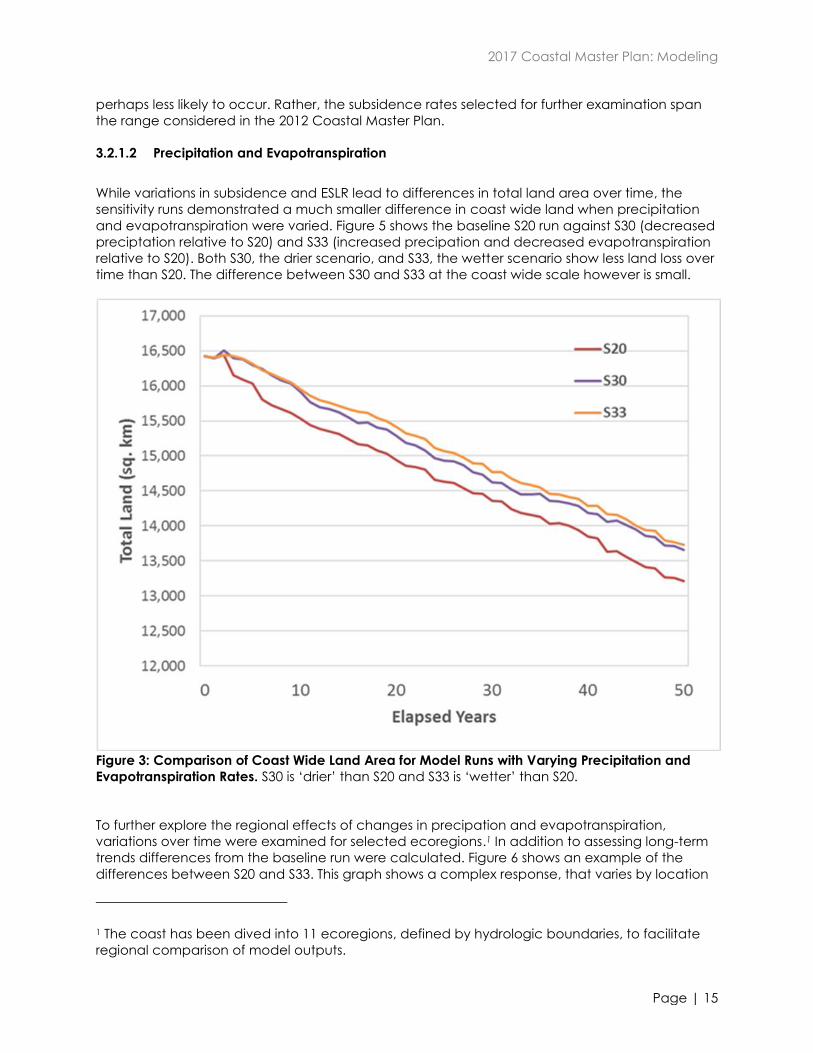
3.2.1.2 Precipitation and Evapotranspiration

While variations in subsidence and ESLR lead to differences in total land area over time, the

sensitivity runs demonstrated a much smaller difference in coast wide land when precipitation

and evapotranspiration were varied. Figure 5 shows the baseline S20 run against S30 (decreased

preciptation relative to S20) and S33 (increased precipation and decreased evapotranspiration

relative to S20). Both S30, the drier scenario, and S33, the wetter scenario show less land loss over

time than S20. The difference between S30 and S33 at the coast wide scale however is small.

Figure 3: Comparison of Coast Wide Land Area for Model Runs with Varying Precipitation and

Evapotranspiration Rates. S30 is ‘drier’ than S20 and S33 is ‘wetter’ than S20.

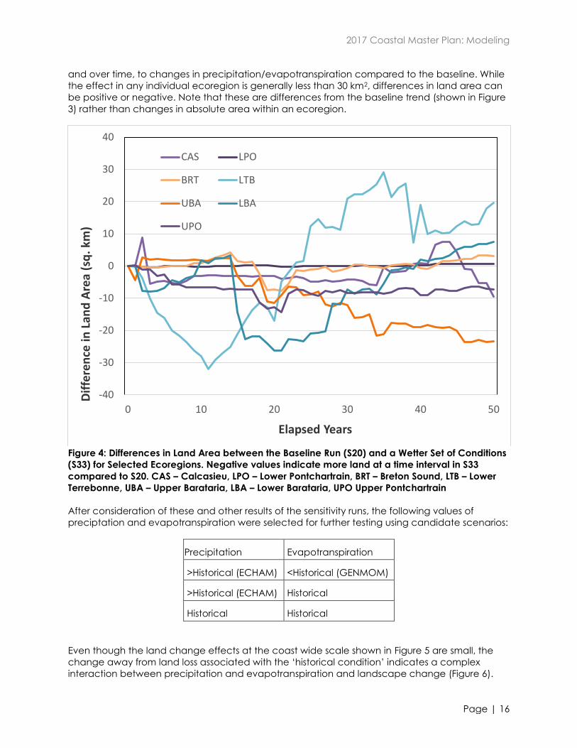
To further explore the regional effects of changes in precipation and evapotranspiration,

variations over time were examined for selected ecoregions.1 In addition to assessing long-term

trends differences from the baseline run were calculated. Figure 6 shows an example of the

differences between S20 and S33. This graph shows a complex response, that varies by location

1 The coast has been dived into 11 ecoregions, defined by hydrologic boundaries, to facilitate

regional comparison of model outputs.


Page | 16

and over time, to changes in precipitation/evapotranspiration compared to the baseline. While

the effect in any individual ecoregion is generally less than 30 km2, differences in land area can

be positive or negative. Note that these are differences from the baseline trend (shown in Figure

3) rather than changes in absolute area within an ecoregion.

Figure 4: Differences in Land Area between the Baseline Run (S20) and a Wetter Set of Conditions

(S33) for Selected Ecoregions. Negative values indicate more land at a time interval in S33

compared to S20. CAS – Calcasieu, LPO – Lower Pontchartrain, BRT – Breton Sound, LTB – Lower

Terrebonne, UBA – Upper Barataria, LBA – Lower Barataria, UPO Upper Pontchartrain

After consideration of these and other results of the sensitivity runs, the following values of

preciptation and evapotranspiration were selected for further testing using candidate scenarios:

Precipitation Evapotranspiration

>Historical (ECHAM) <Historical (GENMOM)

>Historical (ECHAM) Historical

Historical Historical

Even though the land change effects at the coast wide scale shown in Figure 5 are small, the

change away from land loss associated with the ‘historical condition’ indicates a complex

interaction between precipitation and evapotranspiration and landscape change (Figure 6).

-40

-30

-20

-10

0

10

20

30

40

0 10 20 30 40 50

Dif

fere

nce

in L

and

Are

a (s

q. k

m)

Elapsed Years

CAS LPO

BRT LTB

UBA LBA

UPO


Page | 17

The values used are derived from global climate modeling, itself the result of the efforts of a

broad scientific community (Attachment C2-3). Thus, while the effects of varying precipitation

and evapotranspiration may not be large, the inclusion of these variations enables

consideration of complex climate-landscape interactions that may occur in the future.

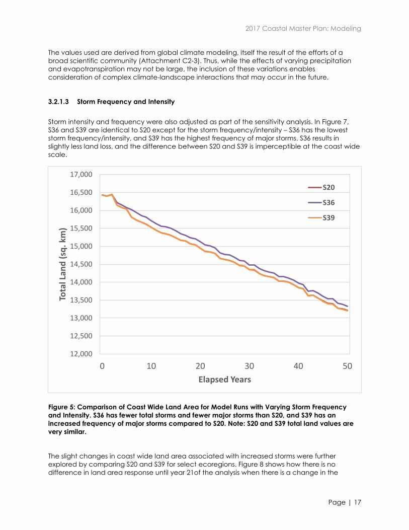
3.2.1.3 Storm Frequency and Intensity

Storm intensity and frequency were also adjusted as part of the sensitivity analysis. In Figure 7,

S36 and S39 are identical to S20 except for the storm frequency/intensity – S36 has the lowest

storm frequency/intensity, and S39 has the highest frequency of major storms. S36 results in

slightly less land loss, and the difference between S20 and S39 is imperceptible at the coast wide

scale.

Figure 5: Comparison of Coast Wide Land Area for Model Runs with Varying Storm Frequency

and Intensity. S36 has fewer total storms and fewer major storms than S20, and S39 has an

increased frequency of major storms compared to S20. Note: S20 and S39 total land values are

very similar.

The slight changes in coast wide land area associated with increased storms were further

explored by comparing S20 and S39 for select ecoregions. Figure 8 shows how there is no

difference in land area response until year 21of the analysis when there is a change in the

12,000

12,500

13,000

13,500

14,000

14,500

15,000

15,500

16,000

16,500

17,000

0 10 20 30 40 50

Tota

l Lan

d (

sq. k

m)

Elapsed Years

S20

S36

S39


Page | 18

character of the storms included in the runs. In that year a storm in S20 is replaced with a

different synthetic storm2 to represent an increase in the frequency of major storms. Changes in

S39 compared to S20 result in more land loss in some ecoregions (e.g., AVB) and less land loss in

others (e.g., UTB). In the ICM, storms can erode barrier islands, introduce sediments to marshes,

and alter salinity and inundation patterns – effects which can be positive or negative for land

area depending on the antecedent conditions. In addition the consequences of the change in

storm are not limited to the year in which the storm occurs as changes in land loss alter

hydrologic exchange in later years. The next change in storm character occurs in year 34 which

triggers a change in land area between S20 and S39 in LTB. Over the 50-year period there are

both positive and negative changes in different areas of the coast resulting in very little change

at the coast wide scale shown in Figure 7, but a substantial change in some areas.

Figure 6: Differences in Land Area between the Baseline Run (S20) and an Increase in the

Number of Total Storms and the Frequency of Major Storms (S39) for Selected Ecoregions.

Negative values indicate more land at a time interval in S39 compared to S20. AVB –

Atchafalaya/Vermilion Bay, CAS – Calcasieu, LPO – Lower Pontchartrain, LTB – Lower Terrebonne,

UBA – Upper Barataria, LBA – Lower Barataria, UTB – Upper Terrebonne

2 See Attachment C3-3 for more details on how synthetic storms were selected for inclusion in

the modeling

-10

-5

0

5

10

15

0 10 20 30 40 50

Dif

fere

nce

in L

and

Are

a (s

q. k

m)

Elapsed Years

AVB CAS

LPO LTB

UBA LBA

UTB


Page | 19

Examination of the sensitivity of land area to changes in storm intensity and frequency showed

that the inclusion (or exclusion) of individual storms over the 50-year period led to substantial

local changes in land area but only to a small effect at the coast wide scale. Further inspection

of land-water maps indicated that some of these local effects were compartment specific (e.g.,

the penetration of salt during a storm resulting in land loss). Because the effects are so localized

and so sensitive to individual storms, it seems possible that varying the number and intensity of

storms among scenarios could subject some projects (e.g., those located in the path of a storm

that was included or excluded) to be impacted based on its location rather than its restoration

characteristics. While this remains an issue to be carefully evaluated even if the storm set stays

the same among the scenarios, varying storms by scenario could make the interpretation of

project results challenging. Thus, the decision was made not to vary storm intensity and

frequency in the landscape analysis.

3.2.2 Evaluation of Candidate Scenarios

Five candidate scenarios were selected for testing to inform the selection of the three

environmental scenarios to be used in the 2017 Coastal Master Plan (Table 7). Due to the small

variation on coast wide land associated with variation in precipitation and evapotranspiration,

only three combinations were tested. These were combined with five combinations of values for

eustatic sea level rise and subsidence.

Table 5: Values Used in the Five Candidate Environmental Scenarios.

Scenario Precipitation Evapotranspiration ESLR (m/50yr) Subsidence

1 >Historical (ECHAM) <Historical

(GENMOM)

0.43 20% of range

2 >Historical (ECHAM) Historical 0.63 50% of range

3 Historical Historical 0.83 50% of range



The results of the candidate scenario testing are shown in Figure 9. As expected based on the

sensitivity analysis, S03, with the highest ESLR and the highest subsidence value, shows the

greatest decrease in land area. S01 with the lowest ESLR and subsidence values shows the

lowest coast wide land loss.


Page | 20

Figure 7: Coast Wide Land Area under Future Without Action for the Five Candidate Scenarios

(see Table 7 for drivers included in each).

3.2.3 Varying Storm Frequency and Intensity in CLARA

The CLARA model implements uncertainty in future storminess using environmental drivers, one

representing the overall frequency of hurricanes impacting the study region and the other

representing the average intensity of those storms. Future scenarios are defined by specifying

changes in those two characteristics, relative to a baseline of current conditions. By contrast, the

ICM models the overall frequency of hurricanes with no change from the historical record and

specifies the frequency of major storms (those with sustained winds of greater than 100 knots).

Separately varying the frequency of all storms and the frequency of major storms implies a

change in the average intensity of storms included in the analysis.

As such, the implementations of future storminess in the CLARA and ICM models are related. Test

runs of the ICM showed that a scenario assumption with the overall frequency of storms

declining by 28% and the frequency of severe storms within the decreased total increasing by

13% over the 50-year simulation period showed little change in the net area of land across the

coast (although there were local changes). Empirical analysis of the National Hurricane Center

4,000

6,000

8,000

10,000

12,000

14,000

16,000

0 10 20 30 40 50

Tota

l Lan

d (

sq. k

m)

Elapsed Years

S01

S02

S03

S04

S05


Page | 21

Data set3 indicates that this is equivalent in CLARA to a 28% decline in storm frequency

combined with a 10% increase in average storm intensity.

Sensitivity testing suggests that modeling variation in both storm frequency and intensity is

important for identifying potential variation in the performance of risk reduction projects. Coast

wide estimates of expected annual damage (EAD) were generated using test data from the

Year 50, 2012 Coastal Master Plan Less Optimistic landscape, varying storm frequency by -5%,

0%, and +5% relative to the historical frequency, and varying average storm intensity by 0%, 10%,

and 20%. (Note that the 0%/0% case is equivalent to seeing no change in storminess compared

to historical conditions, and the 5%/20% case is equivalent to the change in storminess assumed

by the Less Optimistic scenario in 2012.)

Examining the elasticity of damage with respect to the parameters (i.e., the change in EAD

resulting from a percentage change in storm frequency or average intensity) reveals some key

differences:

1. Damage elasticity with respect to average storm intensity appears approximately

constant, with a 10% increase in average intensity producing an 8% increase in EAD.

The elasticity with respect to frequency varies, though; moving from -5% to 0%

increases coast wide EAD by about 4.6%, but going from 0% to 5% increases EAD by

about 8.7%.

2. Changes in storm intensity have a much more pronounced effect on EAD for areas

within the Hurricane Storm Damage Risk Reduction System (HSDRRS), relative to other

areas. A 10% increase in intensity increases EAD by about 15% for points on the East

Bank of New Orleans, and 20% on the West Bank of New Orleans, compared to

increases of 5.5% in other enclosed areas and 6.5% in unenclosed areas. Changes in

storm frequency, on the other hand, produce approximately the same change in

EAD for enclosed and unenclosed points.

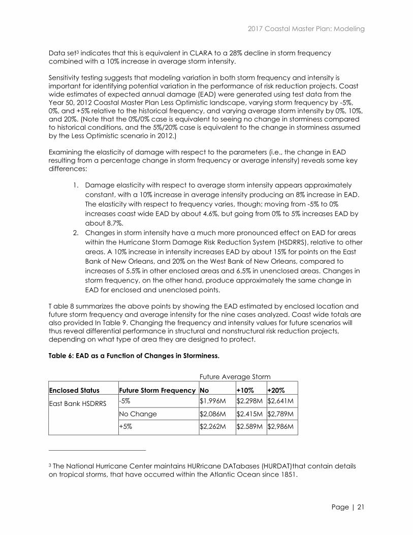
T able 8 summarizes the above points by showing the EAD estimated by enclosed location and

future storm frequency and average intensity for the nine cases analyzed. Coast wide totals are

also provided In Table 9. Changing the frequency and intensity values for future scenarios will

thus reveal differential performance in structural and nonstructural risk reduction projects,

depending on what type of area they are designed to protect.

Table 6: EAD as a Function of Changes in Storminess.

Future Average Storm

Intensity Enclosed Status Future Storm Frequency No

Change

+10% +20%

East Bank HSDRRS -5% $1,996M $2.298M $2,641M

No Change $2,086M $2.415M $2,789M

+5% $2,262M $2.589M $2,986M

3 The National Hurricane Center maintains HURricane DATabases (HURDAT)that contain details

on tropical storms, that have occurred within the Atlantic Ocean since 1851.

https://en.wikipedia.org/wiki/Tropical_cyclone

https://en.wikipedia.org/wiki/Atlantic_Ocean


Page | 22

Future Average Storm

Intensity Enclosed Status Future Storm Frequency No

Change

+10% +20%

West Bank HSDRRS -5% $111M $131M $162M

No Change $119M $144M $177M

+5% $126M $148M $189M

Enclosed, Non-

HSDRRS

-5% $1,550M $1,637M $1,724M

No Change $1,628M $1,713M $1,806M

+5% $1,759M $1,870M $1,996M

Unenclosed -5% $11,147M $11,859M $12,657M

No Change $11,645M $12,400M $13,208M

+5% $12,615M $13,517M $14,474M

Table 7: EAD as a Function of Changes in Storminess - Coast wide Summary.

Future Average Storm Intensity

Future Storm Frequency No

Change

+10% +20%

-5% $14,805M $15,925M $17,184M

No Change $15,479M $16,672M $17,980M

+5% $16,762M $18,124M $19,615M

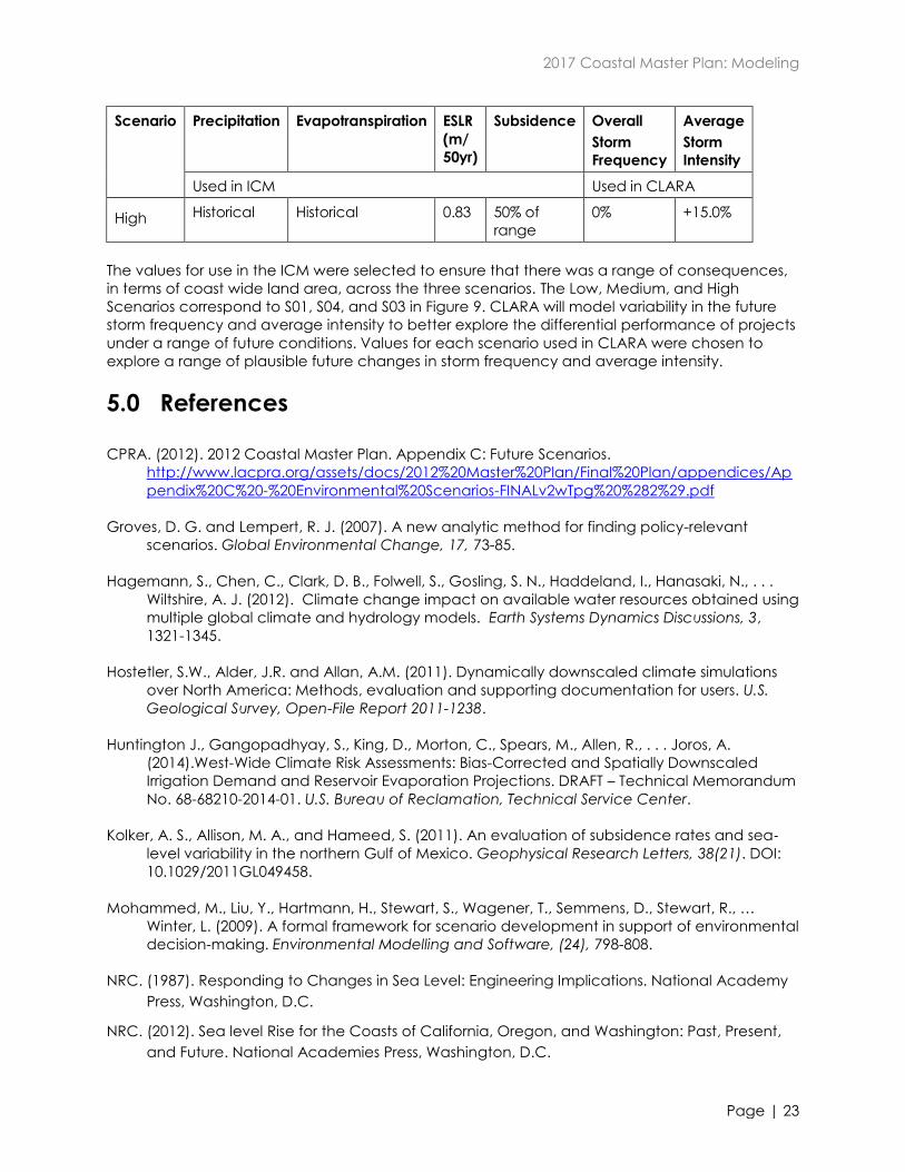
4.0 Selection of Environmental Scenarios

Based on the analysis and testing described above, three environmental scenarios have been

selected for use in the 2017 Coastal Master Plan. The values for these scenarios are shown in

Table 10.

Table 8: Characteristics of the Environmental Scenarios to be used in the 2017 Coastal Master

Plan.

Scenario Precipitation Evapotranspiration ESLR

(m/

50yr)

Subsidence Overall

Storm

Frequency

Average

Storm

Intensity

Used in ICM Used in CLARA

Low >Historical <Historical 0.43 20% of

range

-28% +10.0%

Medium >Historical Historical 0.63 20% of

range

-14% +12.5%


Page | 23

Scenario Precipitation Evapotranspiration ESLR

(m/

50yr)

Subsidence Overall

Storm

Frequency

Average

Storm

Intensity

Used in ICM Used in CLARA

High Historical Historical 0.83 50% of

range

0% +15.0%

The values for use in the ICM were selected to ensure that there was a range of consequences,

in terms of coast wide land area, across the three scenarios. The Low, Medium, and High

Scenarios correspond to S01, S04, and S03 in Figure 9. CLARA will model variability in the future

storm frequency and average intensity to better explore the differential performance of projects

under a range of future conditions. Values for each scenario used in CLARA were chosen to

explore a range of plausible future changes in storm frequency and average intensity.

5.0 References

CPRA. (2012). 2012 Coastal Master Plan. Appendix C: Future Scenarios.

http://www.lacpra.org/assets/docs/2012%20Master%20Plan/Final%20Plan/appendices/Ap

pendix%20C%20-%20Environmental%20Scenarios-FINALv2wTpg%20%282%29.pdf

Groves, D. G. and Lempert, R. J. (2007). A new analytic method for finding policy-relevant

scenarios. Global Environmental Change, 17, 73-85.

Hagemann, S., Chen, C., Clark, D. B., Folwell, S., Gosling, S. N., Haddeland, I., Hanasaki, N., . . .

Wiltshire, A. J. (2012). Climate change impact on available water resources obtained using

multiple global climate and hydrology models. Earth Systems Dynamics Discussions, 3,

1321-1345.

Hostetler, S.W., Alder, J.R. and Allan, A.M. (2011). Dynamically downscaled climate simulations

over North America: Methods, evaluation and supporting documentation for users. U.S.

Geological Survey, Open-File Report 2011-1238.

Huntington J., Gangopadhyay, S., King, D., Morton, C., Spears, M., Allen, R., . . . Joros, A.

(2014).West-Wide Climate Risk Assessments: Bias-Corrected and Spatially Downscaled

Irrigation Demand and Reservoir Evaporation Projections. DRAFT – Technical Memorandum

No. 68-68210-2014-01. U.S. Bureau of Reclamation, Technical Service Center.

Kolker, A. S., Allison, M. A., and Hameed, S. (2011). An evaluation of subsidence rates and sea‐level variability in the northern Gulf of Mexico. Geophysical Research Letters, 38(21). DOI:

10.1029/2011GL049458.

Mohammed, M., Liu, Y., Hartmann, H., Stewart, S., Wagener, T., Semmens, D., Stewart, R., …

Winter, L. (2009). A formal framework for scenario development in support of environmental

decision-making. Environmental Modelling and Software, (24), 798-808.

NRC. (1987). Responding to Changes in Sea Level: Engineering Implications. National Academy

Press, Washington, D.C.

NRC. (2012). Sea level Rise for the Coasts of California, Oregon, and Washington: Past, Present,

and Future. National Academies Press, Washington, D.C.

http://www.lacpra.org/assets/docs/2012%20Master%20Plan/Final%20Plan/appendices/Appendix%20C%20-%20Environmental%20Scenarios-FINALv2wTpg%20%282%29.pdf

http://www.lacpra.org/assets/docs/2012%20Master%20Plan/Final%20Plan/appendices/Appendix%20C%20-%20Environmental%20Scenarios-FINALv2wTpg%20%282%29.pdf


Page | 24

Parris, A., Bromirski, P., Burkett, V., Cayan, D., Culver, M., Hall, J., Horton, R., . . . Weiss, J. (2012).

Global Sea Level Rise Scenarios for the US National Climate Assessment. NOAA Tech Memo

OAR CPO-1. 37 pp.

Sankovich, V., Gangopadhyay, S., Pruitt, T., and Caldwell, R.J. (2013). Los Angeles Basin

Stormwater Conservation Study – Task 3.1 Development of Climate-Adjusted Hydrologic

Model Inputs. U.S. Bureau of Reclamation - Technical Service Center. Denver, Colorado.

USACE. (2009). Water Resources Policies and Authorities Incorporating Sea-Level Change

Considerations into Civil Works Programs (Circular No. 1165-2-211), July 1, 2009, expires July

1, 2011.

USACE. (2011). Sea-Level Change Considerations for Civil Works Programs (Circular No. 1165-2-

212), October 1, 2011, expires September 30, 2013.

Vermeer, M. and Rahmstorf, S. (2009). Global Sea Level Linked to Global Temperature. PNAS

106:51 pp 21527-21532. Published online:

http://www.pnas.org/content/106/51/21527.full.pdf+html

http://www.pnas.org/content/106/51/21527.full.pdf+html

2017 coastal master plan appendix c:...

Documents