Comparison of spatial interpolation methods to create high-resolution poverty maps for low- and middle-income countries

Authors: Kerry LM Wong1* (kerry.wong@lshtm.ac.uk)Oliver J Brady1,2 (oliver.brady@lshtm.ac.uk)Oona MR Campbell1 (oona.campbell@lshtm.ac.uk)Lenka Benova1,3 (lenka.benova@lshtm.ac.uk)

Author information:1 Faculty of Epidemiology and Population Health, London School of Hygiene and Tropical Medicine, Keppel Street, London WC1E 7HT, United Kingdom2 Centre for Mathematical Modelling for Infectious Diseases, London School of Hygiene and Tropical Medicine, Keppel Street, London WC1E 7HT, United Kingdom3 Department of Public Health, Institute of Tropical Medicine, Nationalestraat 155, 2000 Antwerp, Belgium*Author for correspondence

1

Abstract High-resolution poverty maps are important tools for promoting equitable and sustainable development. In settings without data at every location, we can use spatial interpolation (SI) to create such maps using sample-based surveys and additional covariates. In the Model-Based Geostatistics (MBG) framework for SI, it is typically assumed that the similarity of two areas is inversely related to their distance between one another. Applications of spline interpolation takes a contrasting approach that an area’s absolute location and its characteristics are more important for prediction than distance to/characteristics of other locations. This study compares prediction accuracy of the MBG approach with spline interpolation as part of a generalized additive model (GAM) for four low- and middle-income countries. We also identify any potentially generalizable data characteristics influencing comparative accuracy. We found spatially scattered pockets of wealth in Malawi and Tanzania (corresponding to the major cities), and overarching spatial gradients in Kenya and Nigeria. Spline interpolation/GAM performed better than MBG for Malawi, Nigeria and Tanzania, but marginally worse in Kenya. We conclude that the spatial patterns of wealth and other covariates should be carefully accounted for when choosing the best SI approach. This is particularly pertinent as different methods capture geographic variation differently.

KeywordsSpatial interpolation, poverty mapping, wealth inequality, low- and middle-income countries

Media SummaryWe compared two multivariate methods for spatial interpolation to create high-resolution poverty maps in low-data availability settings. These methods differ in how they capture remaining residual spatial correlation after accounting for possible covariate effects. Model-Based Geostatistics assumes such correlation diminishes with increasing distance; spline interpolation considers an area’s absolute location to be more important. Predictors included population density and night-time light emission. In economically multi-centric study regions (e.g., Malawi and Tanzania) the spline formulation generally performed better. Among other important factors identified, the spatial patterns of wealth and other covariates are essential to choosing the best interpolation approach.

2

IntroductionPoverty has strong associations with adverse health outcomes, lost human potential and societal instability1,2. The international community and national governments that signed on to the Sustainable Development Goals are committed to eradicating poverty in all its forms. To achieve this goal, it is helpful to have information on where affected individuals and communities reside at refined spatial scales since aggregate data can conceal heterogeneity and any underlying patterns. Subnational poverty maps that describe spatial patterns of poverty and inequality across a country can help more effectively allocate resources and implement targeted interventions to attain higher levels of wealth and welfare among the most deprived.

Data on poverty indicators at refined geographic scales across a country are regularly collected via censuses. However, decennial censuses are too infrequent to enable timely monitoring and tracking. National surveys are generally more frequent but representative only for coarse spatial units. To overcome these constraints, Elbers and colleagues extended the techniques of small area estimation (SAE) to both types of data in 20003. The SAE method for area-unit mapping identifies comparable census and survey variables, models the desired attribute (e.g. poverty) using the survey variables common to the census, and computes poverty on small geographic partitions (e.g. enumeration area, village or hamlet) across the country based on the model obtained and the census predictor variables. Poverty/welfare is assumed to be uniform within each target region. The method has been widely used to produce subnational choropleth maps of poverty indicators in many low- and middle-income countries (LMICs)4–7. Other areal interpolation techniques include the dasymetric modelling method, which takes advantage of ancillary data to better approximate and redistribute count data within each target area8. This method has been demonstrated for accurate population mapping by age, sex and race9, and may be extended to other socioeconomic characteristics.

The availability of georeferenced data has drastically increased in recent years. The Demographic and Health Survey (DHS) Program, for instance, has gained a reputation for collecting and providing georeferenced data on core development indicators in LMICs over the last few decades. Better data, coupled with new geographic information system (GIS) analytical techniques, has fuelled interests among researchers to improve output quality, including using spatial interpolation (SI) modelling techniques to create high-resolution gridded map surfaces. We assume that the variable of interest (e.g. poverty) has a meaningful value at every location within a study region, which is typically divided into non-overlapping small grid squares. SI techniques are then employed to predict values at every grid based on the sampled data and, where applicable, auxiliary covariates. Many multivariate spatial statistical methods have been applied in studies using DHS georeferenced data for spatial modelling and interpolation, such as SAE, kriging, autoregressive methods and model-based geostatistics (MBG)10. In 2013, The DHS Spatial Interpolation Working Group assessed various properties of these SI methods, e.g., computational efficiency, account for non-stationary variance and inclusion of optimal covariate selection procedures. The Working Group proposed the MBG approach as the most suitable for creating interpolated surfaces10–12. The incorporation of uncertainty into the modelling framework was seen as a compelling strength of MBG10.

In 2014, the WorldPop project and partners pioneered the creation of high-resolution gridded map surfaces of the estimated proportions of people living under the USD1.25 and USD2.00 poverty thresholds with DHS data using a Bayesian Model-Based Geostatistics (MBG) approach13. Poverty map surfaces were drawn for Kenya, Tanzania, Uganda and Pakistan, among others13. Furthermore, maps of population age structure14, fertility indicators15, malaria

3

indicators16,17 and other health indicators (e.g. childhood vaccination, childhood malnutrition, household access to improved source of drinking water and sanitation12,18) were also produced using the same framework.

The MBG methodology is detailed elsewhere19. Briefly, it divides spatial variation into three components – deterministic variation, spatial autocorrelation and random noise20. The deterministic variation of the phenomenon of interest is modelled as a set of covariates, whilst spatial autocorrelation refers to a variable’s relationship with itself in space21. It is generally assumed that nearer neighbours are more related to each other than more distant counterparts. Such positive autocorrelation structure is defined and used as part of the MBG approach to explain variation in the data and make more accurate predictions at unsampled locations across the map region. Non-stationarity and other localized effects can be dealt with when implementing MBG via, for instance, optimal estimation of the covariance matrix or a Bayesian Partition Model22, but the method remains most widely used for phenomena that are more similar as a function of the distance separating the sampled locations in practice23–25.

On the other hand, spline interpolation is grounded in a slightly different theoretical viewpoint. Spline interpolation assumes that the interpolation function should pass through (or close to) the data points whilst being as smooth as possible. Spline interpolation can be conceptualized as bending a sheet of rubber through the observations in three-dimensional space. In this method, the geographic structure of the mapped phenomenon is not explicitly formulated. Researchers have incorporated spline spatial interpolation in a generalized additive model (GAM) formulation with the geographic coordinates (e.g. longitude and latitude) and other covariates to create interpolated map surfaces. In this GAM framework, each predictor variable is related to the outcome via a smoothed function, then all functions are added to predict the link function. Insurance pricing26, property pricing27, lexical data28 and fish ecology29,30, just to name a few different outcomes, have been mapped using this robust method in the literature.

The assumptions about the underlying variation in the sampled data, the choice of method and the parameters used can be critical to SI prediction accuracy20. Individuals and households with common characteristics sometimes cluster together either by choice or due to social, economic, geographic or political forces31. The assumption of spatial autocorrelation in wealth may be valid, as poverty tends to concentrate in mountainous regions, arid land, land-locked areas, and levels-off closer to the national/financial capitals, bodies of water and coastal areas32. In recent years however, the emergence of secondary cities in many LMICs may have led to certain degree of within-country redistribution of the population, economic opportunities and wealth33. Secondary cities are fast-developing regional hubs that provide critical support functions for governance, production services and transportation. Sometimes the locations of these cities are deliberately planned for deprived regions. Thus, a rather complex spatial structure of towns and cities might be expected, and raises concerns regarding the quality of interpolation when (positive) spatial autocorrelation is assumed and used for prediction making.

The way in which wealth is distributed across the map region likely affects prediction accuracy of the poverty maps made using existing SI approaches to different extents. We present an analysis comparing the performance of spline interpolation as part of GAM-based fitting with multivariate MBG for four LMICs in sub-Saharan Africa. The result of this comparative analysis will empirically reveal the data characteristics that contribute to any discrepancies in prediction accuracy found between methods. This will in turn shed light on the suitability of the two methods for the creation of interpolated poverty maps.

4

5

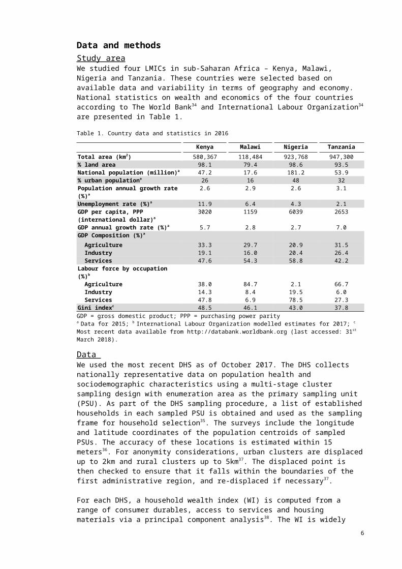
Data and methodsStudy areaWe studied four LMICs in sub-Saharan Africa – Kenya, Malawi, Nigeria and Tanzania. These countries were selected based on available data and variability in terms of geography and economy. National statistics on wealth and economics of the four countries according to The World Bank34 and International Labour Organization34 are presented in Table 1. Table 1. Country data and statistics in 2016

Kenya Malawi Nigeria TanzaniaTotal area (km2) 580,367 118,484 923,768 947,300% land area 98.1 79.4 98.6 93.5National population (million)a 47.2 17.6 181.2 53.9% urban populationa 26 16 48 32Population annual growth rate (%)a

2.6 2.9 2.6 3.1

Unemployment rate (%)a 11.9 6.4 4.3 2.1GDP per capita, PPP (international dollar)a

3020 1159 6039 2653

GDP annual growth rate (%)a 5.7 2.8 2.7 7.0GDP Composition (%)a

Agriculture 33.3 29.7 20.9 31.5 Industry 19.1 16.0 20.4 26.4 Services 47.6 54.3 58.8 42.2Labour force by occupation (%)b

Agriculture 38.0 84.7 2.1 66.7 Industry 14.3 8.4 19.5 6.0 Services 47.8 6.9 78.5 27.3Gini indexc 48.5 46.1 43.0 37.8GDP = gross domestic product; PPP = purchasing power paritya Data for 2015; b International Labour Organization modelled estimates for 2017; c Most recent data available from http://databank.worldbank.org (last accessed: 31st March 2018).

Data We used the most recent DHS as of October 2017. The DHS collects nationally representative data on population health and sociodemographic characteristics using a multi-stage cluster sampling design with enumeration area as the primary sampling unit (PSU). As part of the DHS sampling procedure, a list of established households in each sampled PSU is obtained and used as the sampling frame for household selection35. The surveys include the longitude and latitude coordinates of the population centroids of sampled PSUs. The accuracy of these locations is estimated within 15 meters36. For anonymity considerations, urban clusters are displaced up to 2km and rural clusters up to 5km37. The displaced point is then checked to ensure that it falls within the boundaries of the first administrative region, and re-displaced if necessary37.

For each DHS, a household wealth index (WI) is computed from a range of consumer durables, access to services and housing materials via a principal component analysis38. The WI is widely adopted in LMICs as an indicator of socioeconomic position that describes a household's cumulative living standard within an individual survey39. The index also is broadly used for assessing pro-poor targeting and inequality, and, where relevant, for controlling for socioeconomic confounding40. To approximate poverty at the PSU level, we used the average household WI (rescaled by a factor of 10-6) with adjustment for survey-specific weights as outlined by DHS manuals. We present descriptive results of the data distribution and spatial pattern of WI of the four study countries.

Model covariates We identified and assembled a collection of remote sensing covariates based on those used by others to generate maps of multidimensional poverty13. In

6

general, the accuracy of these data to provide up-to-date indication on welfare and living conditions is considered acceptable13,41–45. We included data on population density from version four of the Gridded Population of the World (GPW)46, on daytime land surface temperature47 and vegetation index48 from the NASA Earth Observations (NEO), on elevation data from the United States Geological Survey (USGS)49, rasterized surfaces of Global Potential evapo-transpiration and Global Aridity Index from the Consortium for Spatial Information at the Consultative Group for International Agricultural Research (CGIAR-CSI)50–52, and on night-time light emission from the National Oceanic and Atmospheric Administration (NOAA)/National Geophysical Data Center by the United States Air Force Weather Agency53,54. At their finest resolutions, the land surface temperature layer and the vegetation index layer were 0.1 degree grids (approximately 11km at the equator), while the other covariate layers were 30 arc second grids (approximately 1km at the equator). Using these files, we extracted covariate values from each raster layers at the georeferenced PSUs, represented as spatial points, via spatial overlaying55. That is, we superimposed a spatial layer of the georeferenced PSUs over different covariate layers and obtained covariate values at the corresponding locations. To account for PSU location displacement, averages were obtained from the four nearest raster cells. As a check of sensitivity to alternative analytical scales, these averages were compared to those resulting from applying buffer sizes of 5km, 10km and 20km using Pearson correlation coefficients.

We updated accessibility measures for the current analysis with Natural Earth’s free data on “populated places” (version 4.0.0, released in October 2017), which included national and subnational capitals, as well as places with a population size of at least 50,00056. We calculated the straight-line distance from every included DHS PSU to the nearest populated place. We opted for straight-line distance for its comparability to proxy accessibility with more complicated metrics such as mechanized and non-mechanized estimated travel time in LMIC settings57. Country administrative areas shapefiles were obtained from the freely available Database of Global Administrative Areas58.

We found missing data in the spatial coordinates of 9 of 1594 PSUs from the Kenya DHS and 7 of 896 PSUs from the Nigeria DHS. These PSUs were removed from the analysis59. There were no other missing data. In addition, one PSU data point was removed from the analysis in the Southern Region in Malawi as it had an extreme value of 41453 for population density, whilst the median and 75th percentile were 267 and 579 and observations of the nearest neighbours were below 10000.

Methods of interpolationModel-based geostatistics (MBG)The MBG model is a class of generalized linear mixed models with an approximation of a multivariate stationary Gaussian Process for outcome z at location si with mean μ and covariance C for the spatial component, as well as an unstructured component ε(si) represented as Gaussian with zero mean and variance19. The mean μ is modelled using a linear function of the predictor variables, whilst spatial covariance is written as C(Z(s1), Z(s2)) = E[(Z(s1) – μ) (Z(s2) – μ)]where s1 and s2 are a pair of sampled locations of distance h units apart. Covariance expresses the amount of variation in the observed Z values at s1 and s2. We separately modelled the spatial dependency structure using a spherical covariance function for each included survey. The spherical covariance function is written as ρ(h): C(h) = σ2ρ(h), where

7

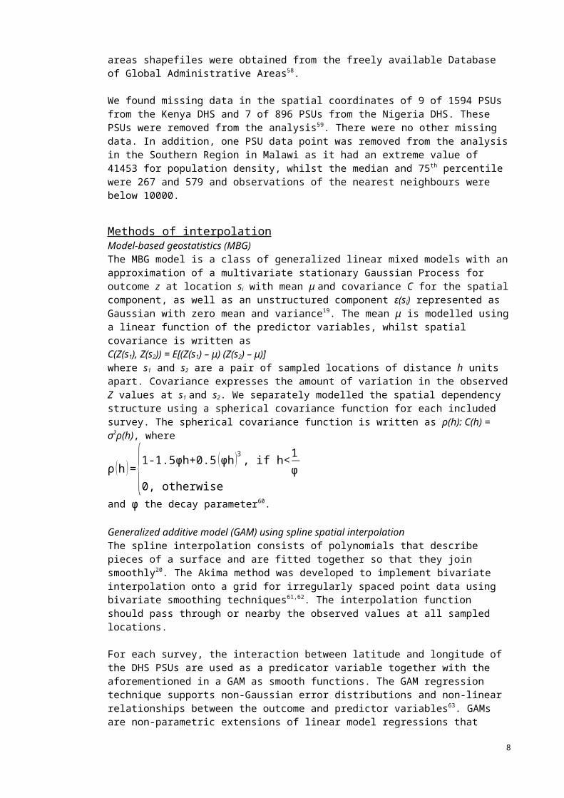
ρ (h ) ={1-1.5ϕh+0.5 (ϕh )3 , if h< 1ϕ

0, otherwiseand ϕ the decay parameter60.

Generalized additive model (GAM) using spline spatial interpolationThe spline interpolation consists of polynomials that describe pieces of a surface and are fitted together so that they join smoothly20. The Akima method was developed to implement bivariate interpolation onto a grid for irregularly spaced point data using bivariate smoothing techniques61,62. The interpolation function should pass through or nearby the observed values at all sampled locations.

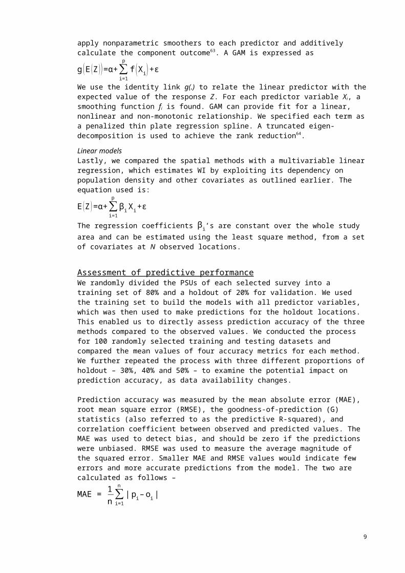
For each survey, the interaction between latitude and longitude of the DHS PSUs are used as a predicator variable together with the aforementioned in a GAM as smooth functions. The GAM regression technique supports non-Gaussian error distributions and non-linear relationships between the outcome and predictor variables63. GAMs are non-parametric extensions of linear model regressions that apply nonparametric smoothers to each predictor and additively calculate the component outcome63. A GAM is expressed as

g ( E (Z ) ) =α+∑i=1

p

f (X i )+ε

We use the identity link g(.) to relate the linear predictor with the expected value of the response Z. For each predictor variable Xi, a smoothing function fi is found. GAM can provide fit for a linear, nonlinear and non-monotonic relationship. We specified each term as a penalized thin plate regression spline. A truncated eigen-decomposition is used to achieve the rank reduction64. Linear modelsLastly, we compared the spatial methods with a multivariable linear regression, which estimates WI by exploiting its dependency on population density and other covariates as outlined earlier. The equation used is:

E (Z )=α+∑i=1

p

βi Xi +ε

The regression coefficients β i’s are constant over the whole study area and can be estimated using the least square method, from a set of covariates at N observed locations. Assessment of predictive performanceWe randomly divided the PSUs of each selected survey into a training set of 80% and a holdout of 20% for validation. We used the training set to build the models with all predictor variables, which was then used to make predictions for the holdout locations. This enabled us to directly assess prediction accuracy of the three methods compared to the observed values. We conducted the process for 100 randomly selected training and testing datasets and compared the mean values of four accuracy metrics for each method. We further repeated the process with three different proportions of holdout – 30%, 40% and 50% – to examine the potential impact on prediction accuracy, as data availability changes.

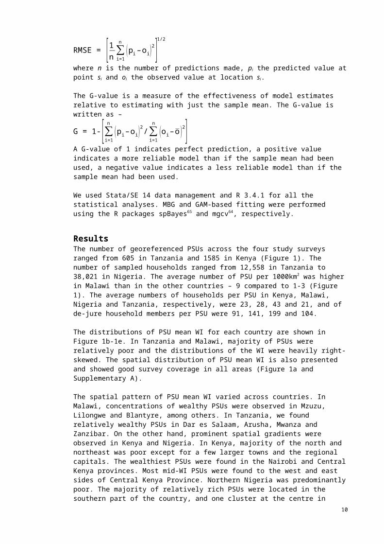
Prediction accuracy was measured by the mean absolute error (MAE), root mean square error (RMSE), the goodness-of-prediction (G) statistics (also referred to as the predictive R-squared), and correlation coefficient between observed and predicted values. The MAE was used to detect bias, and should be zero if the predictions were unbiased. RMSE was used to measure the average magnitude of the squared error. Smaller MAE and RMSE values would indicate

8

few errors and more accurate predictions from the model. The two are calculated as follows –

MAE = 1n ∑

i=1

n

| pi – o i |

RMSE = [1n ∑i=1

n

(p i – oi )2]

1/2

where n is the number of predictions made, pi the predicted value at point si and oi the observed value at location si.

The G-value is a measure of the effectiveness of model estimates relative to estimating with just the sample mean. The G-value is written as –

G = 1-[∑i=1

n

( pi –o i )2 /∑

i=1

n

( oi – o )2]A G-value of 1 indicates perfect prediction, a positive value indicates a more reliable model than if the sample mean had been used, a negative value indicates a less reliable model than if the sample mean had been used.

We used Stata/SE 14 data management and R 3.4.1 for all the statistical analyses. MBG and GAM-based fitting were performed using the R packages spBayes65 and mgcv64, respectively.

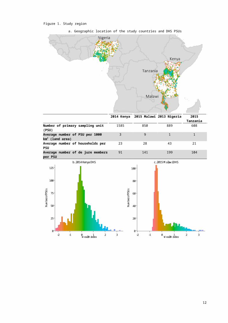
ResultsThe number of georeferenced PSUs across the four study surveys ranged from 605 in Tanzania and 1585 in Kenya (Figure 1). The number of sampled households ranged from 12,558 in Tanzania to 38,021 in Nigeria. The average number of PSU per 1000km2 was higher in Malawi than in the other countries – 9 compared to 1-3 (Figure 1). The average numbers of households per PSU in Kenya, Malawi, Nigeria and Tanzania, respectively, were 23, 28, 43 and 21, and of de-jure household members per PSU were 91, 141, 199 and 104.

The distributions of PSU mean WI for each country are shown in Figure 1b-1e. In Tanzania and Malawi, majority of PSUs were relatively poor and the distributions of the WI were heavily right-skewed. The spatial distribution of PSU mean WI is also presented and showed good survey coverage in all areas (Figure 1a and Supplementary A).

The spatial pattern of PSU mean WI varied across countries. In Malawi, concentrations of wealthy PSUs were observed in Mzuzu, Lilongwe and Blantyre, among others. In Tanzania, we found relatively wealthy PSUs in Dar es Salaam, Arusha, Mwanza and Zanzibar. On the other hand, prominent spatial gradients were observed in Kenya and Nigeria. In Kenya, majority of the north and northeast was poor except for a few larger towns and the regional capitals. The wealthiest PSUs were found in the Nairobi and Central Kenya provinces. Most mid-WI PSUs were found to the west and east sides of Central Kenya Province. Northern Nigeria was predominantly poor. The majority of relatively rich PSUs were located in the southern part of the country, and one cluster at the centre in Abuja. In the south, a substantial number of mid-WI PSUs were seen the Enugu and Makurdi states.

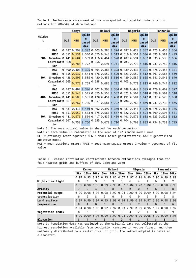
Table 2 shows the four accuracy metrics for all results. Across all study countries, both SI approaches performed better than the linear fit. For both MBG and GAM, mean errors generally increased from lower to higher holdout proportions, and the opposite was observed for G-value and correlation. This indicated a greater probability that inaccurate predictions occurred in models with larger holdouts. Regardless of the SI method used, G-value and correlation

9

were the lowest for Malawi which reflected worst prediction effectiveness when compared with the other three countries.

The GAM fit performed better at all holdout proportions for Malawi, Nigeria and Tanzania based on all four metrics. In Kenya, mixed results were observed – MBG interpolations were comparatively better for RMSE, G-value and correlation between predicted WI and observed WI at 20%-40% holdout. The relative performance of the GAM in Kenya improved as holdout proportions increased to 50%.

The spatial patterns of the covariates are illustrated in Supplementary B, and we explored the effects of the covariates by country using the full datasets (Supplementary C). Night-time light emission most consistently showed an association with WI across all countries, followed by population density. Overall, night-time light was positively associated with WI, whilst the opposite was observed for population density. In the GAM fits, in all cases except for population density in Tanzania, the curves were significant at the 0.001% level. Finally, Pearson correlation coefficients between the average values used for our analysis and those resulting from using buffer sizes of 5km, 10km and 20km showed strong correlations across different extractions methods (Table 3), thus we do not expect the analytical results to differ by using alternative scales.

10

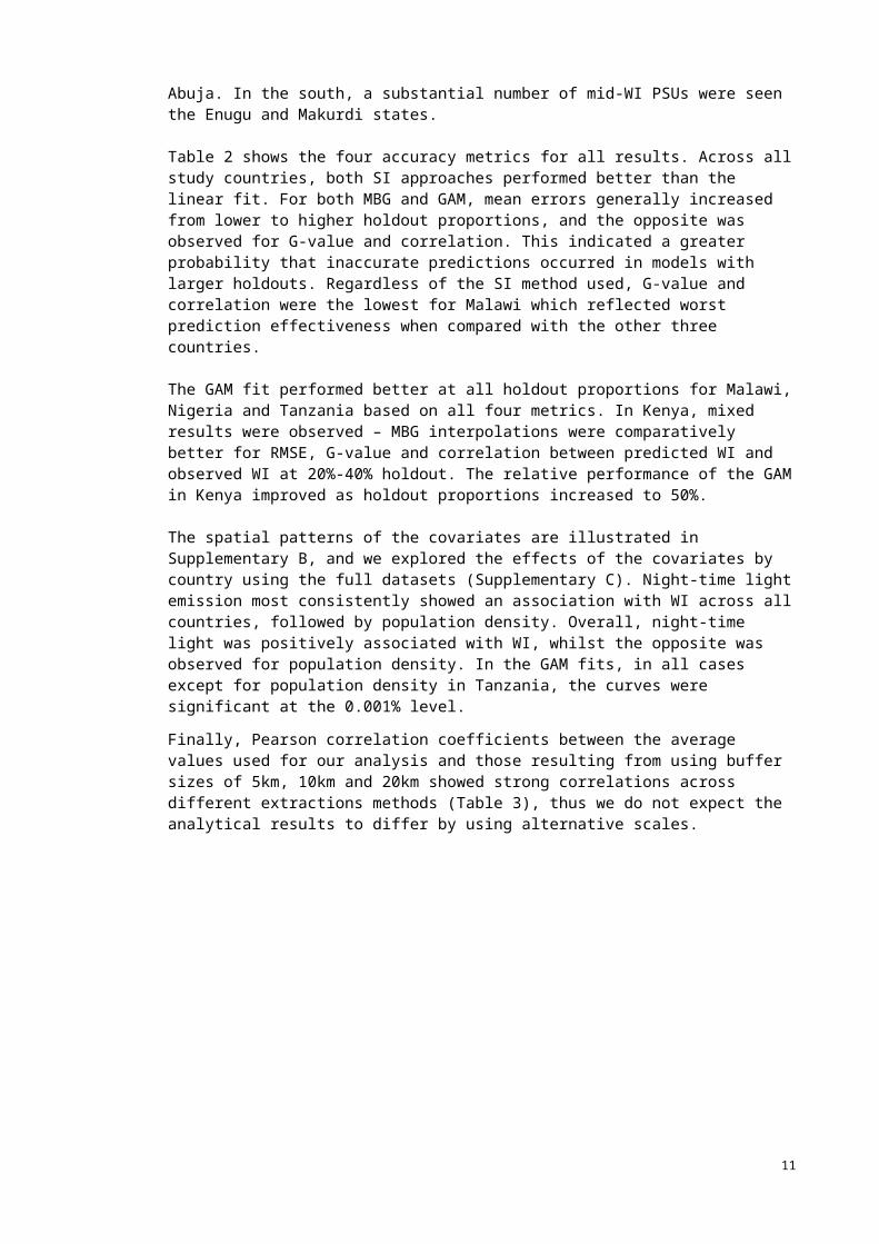
Figure 1. Study region a. Geographic location of the study countries and DHS PSUs

2014 Kenya 2015 Malawi 2013 Nigeria 2015 Tanzania

Number of primary sampling unit (PSU)

1585 850 889 608

Average number of PSU per 1000 km2 (land area)

3 9 1 1

Average number of households per PSU

23 28 43 21

Average number of de jure members per PSU

91 141 199 104

0

25

50

75

100

125

Numb

er of

PSUs

-2 -1 0 1 2 3Wealth index

b. 2014 Kenya DHS

0

20

40

60

80

100

Numb

er of

PSUs

-2 -1 0 1 2 3Wealth index

c. 2015 Malawi DHS

11

0

10

20

30

40

Numb

er of

PSUs

-2 -1 0 1 2 3Wealth index

d. 2013 Nigeria DHS

0

10

20

30

40

50

Numb

er of

PSUs

-2 -1 0 1 2 3Wealth index

e. 2015 Tanzania DHS

Note: The original values of wealth index have been rescaled by a factor of 10-6.

12

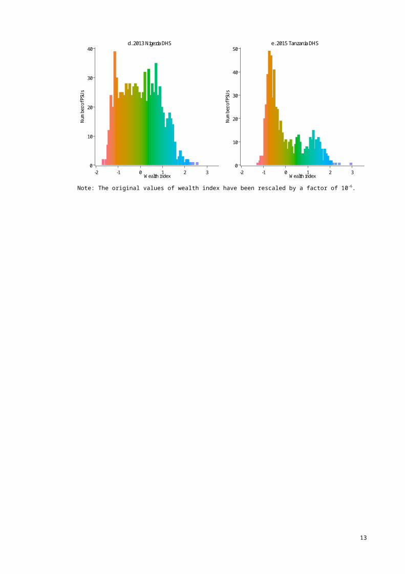
Table 2. Performance assessment of the non-spatial and spatial interpolation methods for 20%-50% of data holdout.

Holdout

Kenya Malawi Nigeria Tanzania

OLS MBGSplin

e basedGAM

OLS MBGSplin

e basedGAM

OLS MBGSplin

e basedGAM

OLS MBGSplin

e basedGAM

20%

MAE 0.487 0.399 0.392 0.403 0.385 0.324 0.487 0.429 0.387 0.475 0.453 0.364RMSE 0.651 0.531 0.540 0.575 0.548 0.513 0.619 0.551 0.506 0.595 0.581 0.499

G-value 0.441 0.604 0.589 0.416 0.464 0.528 0.487 0.594 0.657 0.535 0.535 0.656Correlat

ion0.668 0.780 0.772 0.656 0.691 0.741 0.703 0.775 0.816 0.737 0.742 0.816

30%

MAE 0.490 0.403 0.395 0.404 0.388 0.328 0.489 0.435 0.391 0.478 0.458 0.371RMSE 0.655 0.537 0.544 0.576 0.552 0.520 0.623 0.559 0.512 0.597 0.584 0.509

G-value 0.438 0.596 0.585 0.420 0.456 0.516 0.489 0.587 0.655 0.541 0.541 0.649Correlat

ion0.665 0.775 0.769 0.658 0.685 0.732 0.703 0.771 0.813 0.740 0.744 0.812

40%

MAE 0.487 0.407 0.396 0.402 0.393 0.334 0.488 0.440 0.395 0.479 0.462 0.377RMSE 0.651 0.543 0.545 0.575 0.558 0.537 0.622 0.564 0.518 0.599 0.591 0.518

G-value 0.441 0.585 0.581 0.420 0.451 0.488 0.491 0.581 0.647 0.537 0.529 0.638Correlat

ion0.667 0.767 0.766 0.657 0.681 0.722 0.704 0.766 0.809 0.737 0.736 0.805

50%

MAE 0.487 0.413 0.400 0.402 0.397 0.340 0.487 0.446 0.399 0.478 0.465 0.385RMSE 0.651 0.552 0.553 0.575 0.565 0.547 0.622 0.571 0.524 0.599 0.594 0.531

G-value 0.441 0.571 0.569 0.417 0.437 0.469 0.491 0.571 0.638 0.533 0.521 0.612Correlat

ion0.667 0.758 0.760 0.655 0.672 0.710 0.704 0.760 0.803 0.734 0.731 0.795

Note 1: The more optimal value is shaded for each comparison.Note 2: Each value is calculated as the mean of 100 random model runs.OLS = ordinary least squares; MBG = Model-based geostatistics; GAM = generalized additive modelMAE = mean absolute error; RMSE = root-mean-square error; G-value = goodness of fit value

Table 3. Pearson correlation coefficients between extractions averaged from the four nearest grids and buffers of 5km, 10km and 20km

  Kenya Malawi Nigeria Tanzania

  5km 10km

20km 5km 10k

m20km 5km 10k

m20km 5km 10k

m20km

Night-time light 0.978 0.933 0.859 0.958 0.863 0.673 0.976 0.914 0.802 0.966 0.891 0.812Aridity 0.997 0.989 0.964 0.995 0.988 0.974 1.000 1.000 1.000 0.996 0.983 0.958Potential evapo-transpiration 0.996 0.989 0.968 0.989 0.970 0.940 1.000 0.999 0.999 0.995 0.982 0.948Land surface temperature 0.978 0.994 0.970 0.956 0.988 0.946 0.995 0.997 0.972 0.960 0.986 0.906Vegetation index 0.948 0.988 0.961 0.926 0.979 0.933 0.974 0.992 0.961 0.928 0.982 0.929Elevation 0.998 0.994 0.984 0.990 0.974 0.949 0.996 0.991 0.984 0.998 0.993 0.981Note 1: Population data was excluded as the original data was collected at the highest resolution available from population censuses in vector format, and then uniformly distributed to a raster pixel or grid. The method adopted is detailed elsewhere46.

13

DiscussionIn this study, we assessed the performances of two spatial methods to predict poverty for four countries in sub-Saharan Africa. We compared a Bayesian multivariable MBG approach with spline interpolation as part of a GAM to predict WI at holdout locations using DHS data. We observed better predictive performances of these spatial methods when compared to non-spatial models. Our results revealed marked differences in the shape of the distribution and spatial pattern of WI across the four countries. We found that predictive performance was the lowest in Malawi compared to the other three countries regardless of the method used. GAM-based fitting of smoothed functions of the spatial coordinates and WI, adjusted for other predictor variables, generally performed better than MBG in Malawi, Nigeria and Tanzania. In Kenya, on the other hand, the GAM fit resulted in marginally worse prediction accuracy than the MBG approach. Study limitationsOur findings have important implications but should be understood within certain limitations. First, the random displacement applied to the GPS coordinates of the DHS PSUs could have misclassified assignment of predictor variables66. The extent of misclassification depends on the smoothness of the surface from which data are being linked66. We attempted to mitigate the effects of potential bias of rough/unsmooth surfaces by integrating from raster cells close to the displaced locations. Second, as we conducted an out-of-sample validation based on sampled data, the comparative performance between MBG and GAM if 100% of the data were used to make predictions at unsampled locations is uncertain. Third, we did not use the revised global map of travel time to cities estimated by Weiss and colleagues67 which was published after we analysed our data. Fourth, we opted for a straight-line measure for accessibility as it is unclear that more sophisticated methods are better57,68. Fifth, the use of asset-based indices to assess poverty may be affected by the choice of components and poor comparability between urban and rural areas69,70, but such indices are easy to compute and compare well to more complex indicators of wealth71–73. Sixth, we only used four case countries, and our results may have limited generalizability to LMICs. Last, the wealth index data used for modelling were aggregated to the PSU from household-level data, and the covariates exploited were provided at different grid sizes. Grid size of the land surface temperature layer and the vegetation index layer, in particular, are larger and have potential within-grid variations that cannot be accounted for in the current analysis.MBG and GAMComparison based on goodness-of-fit value and correlation showed that predictive performance was lowest in Malawi, indicating neither model was sufficient to address the spatial variability of WI. The covariate datasets used were provided as raster objects at set grid size. Within each grid, covariate values are considered constant. Given that Malawi has a substantially smaller land area compared to the other three countries, every grid on a Malawi’s covariate layer covers a larger proportion of the country’s surface area, leading to higher levels of aggregation. At higher levels of aggregation, there is greater potential for information loss74. Night-time light emission, one of the strongest predictors found in this study (see Supplementary C), ranged between zero to approximately 60 units across all four countries. If the spatial scale of covariate effect in Malawi was also similar to the other countries, higher levels of aggregation may not lead to greater information loss. On the other hand, if the spatial scale of covariate effect for night-time light in the smaller country and economy was as least as rapid as the other three countries, greater potential for information loss might be expected74. This may have contributed to the reduced model performance and prediction accuracy in Malawi.

14

While the two SI methods explored in this analysis offer different ways to capturing the underlying spatial pattern, they share certain mathematical connection as previously discussed by Cressie and Wahba75,76. Cressie, for instance, demonstrated commonalities between the two-dimensional Laplacian smoothing spline of degree two and the universal kriging predictor76. Nonetheless, the two methods remain “practically very different”76, and the predictive performances resulting from the typical ways in which these methods are applied are the main interest of the current analysis.

Many factors affect the predictive performance of different SI methods, and our study did not yield a consistent “best method”. Rather, each approach offers different ways to capturing different data structure, and in line with previous studies77–79, we found different methods performed better under different conditions. Our results revealed four possible factors to the performance of the methods: 1) data density, 2) normality of data, 3) the underlying spatial wealth pattern and 4) the choice of covariates.

Firstly, the comparative performance of the two approaches might be sensitive to data density. Our results across a range of holdout proportions demonstrated that predictive performances reduced for both methods when sparse datasets were used. Whilst this may not be surprising, the more optimal SI method for Kenya changed from MBG to GAM when data density decreased from 80% to 50%.

Secondly, non-spatial exploratory data analysis indicated that the WI values at the PSU level for Kenya (Figure 1b) followed a normal distribution. On the other hand, the distributions for Malawi, Nigeria and Tanzania were right-skewed (Figure 1c-1e). This empirical difference across countries coincided with MBG performing more optimally for Kenya. Although normality in the outcome is not required for MBG, second order variation is structured as a multivariate normal-distributed random field. The influence of data normality, together with the choice of covariates (more below), on the suitability of different SI methods should be carefully accounted for. This may be particularly pertinent as top inequality – large and slowly declining top wealth shares as indicated by right skew – is rising both globally and in many countries80–82. It is also unlikely to be solely due to our use of WI as a measure of wealth, since previous studies have also found a similar distribution in other wealth indicators in Malawi83 and Tanzania84.

Thirdly, the underlying spatial pattern in the data is important to choosing the “best” performing SI method in a given map region. MBG predictive maps are typically based on the assumptions of stationarity of the spatial process, as the approach accounts for the covariance of the residuals between any two locations by modelling it as dependent on the distance and direction between them, and is independent of the location itself. In the presence of good global spatial autocorrelation, such as the case of Kenya, where the global spatial pattern of wealth appears to decrease over distance from Nairobi (Figure 1a), MBG performed marginally better than GAM. In 1969, the post-colonial Kenyan Government selected seven cities around Nairobi to develop as secondary cities to decongest urban conditions85. While Nairobi remains economic dominant in Kenya, the seven cities have developed a sizable economic base over the last few decades85. Except for Mombasa, these cities span across the Kenyan savannah in the south-west86. The rest of the country is predominately arid land where livelihoods are generally challenging87,88. The geographic pattern of wealth in Kenya may thus be more parsimoniously explained by spatial autocorrelation compared to the other study countries. The tendency for poverty rates to be more similar in nearby locations has also been shown in other LMICs89,90.

15

In other settings, pairs of locations distant from each other may be more similar than nearby neighbours although local spatial autocorrelation is observed, in which case the assumption of stationarity may not be optimal when considering spatial processes over the whole map region. One practical way to take non-stationarity into account in an MBG framework is by partitioning the study area into disjoint regions and define a separate stationary process in each region91. Other non-stationary models may also be appropriate. The GAM formulation, for instance, allows the outcome to vary smoothly in space instead of assuming locations’ predictive power on one another to be dependent on distance. In our study, the GAM approach provided better predictions than MBG at all holdout proportions for Malawi and Tanzania, where we observed spatial scatter of concentrations of wealthy locations across the national extents. The pattern observed in Malawi and Tanzania may not be unique. In Ethiopia and Rwanda, for instance, a secondary cities development component involving collections of locations that form a spatially multi-centred network has been proposed as part of a strategy to attain inclusive growth and build resilience92,93. The identification and inclusion of these secondary cities were partially based on their institutional capacity at the time of selection. Moreover, there were also the intentions to relieve urban conditions in primary cities, promote a spatial balance and equity and transform the economic geography of the countries through redistributing resources92,93. As development of secondary cities continues to be the focus of sustainable growth, it is important to account for the geographic organization of these emerging cities when constructing smoothed map surfaces of wealth and other development indicators using SI techniques. Researchers, planners and development agencies have conceived several types of theoretical city/settlement patterns, including nucleated, clustered, dispersed and random33,94,95. Depending on the spatial processes of the outcome and available covariates, the assumption of spatial stationarity in the SI model formulation may or may not be suitable. The potentials for the similarities between a distant pair of locations, or any pair of locations, to be used as an input for poverty mapping warrant further research. In particular, the application of some non-spatial methods for interpolation, including machine learning techniques, without the constraint of using neighbouring data to make prediction at an unsampled or unobserved location offers new opportunities to capturing more complex spatial patterns41. With these methods, an algorithm is used to decide which observations should be leveraged for a certain prediction, allowing the inclusion of data from any other sample points if the model find them similar to the location being interpolated in terms of the predictor variables.

Lastly, the choice of predictor variables and their relationships with the outcome is a strong factor influencing the predictive performance and the choice of SI method. The outcome being mapped may be spatially correlated, and largely due to certain spatial trends in the covariates. In which case, accounting for covariate effects and examining whether any residual spatial correlation remains are crucial. The current analysis was performed using the full model formulation with all covariates included. Overall, the curvatures for night-time light emission and population density showed the strongest effects across study countries, whilst the other climatic and environmental features have moderate effects in Kenya and Nigeria, and weak effects in Malawi and Tanzania. This is an important point to note for two reasons: 1) the spatial processes of WI in Malawi and Tanzania are less stationary compared to Kenya and Nigeria and 2) remotely sensed data are generally less costly to collect on a vast scale compared to other data collection efforts, making them suitable for the use of SI, but their availability is usually higher for natural conditions in LMICs where the determinants of the spatial structure of wealth are becoming more complex. Non-stationary spatial processes that lack suitable and readily available predictors (e.g., wealth/poverty in Malawi and Tanzania) can limit the predictive performance of SI methods that rely on good spatial stationarity. Different

16

groups around the world are working on producing high resolution data on “man-made” features for large geographic areas – anonymised mobile data96, human settlement pattern97, urban-rural classification97, which are potentially more closely associated with the spatial process of wealth for some settings. Although mostly confined to smaller geographic areas such as subnational administrative regions, the number of studies on high or very high resolution of urban slum mapping have also been increasing98. The use of these data as covariates may mean that spatial autocorrelation would become more or less informative, and have potential influence on the comparative performance of different SI methods. In future attempts to create a smoothed poverty surface for a given region, one may wish to explore method-specific, contextually relevant covariates/interactions, perform variable selection as well as allowing for a more flexible predictor-outcome structure to find the best SI method and model formulation.

ConclusionMBG and spline interpolation offer different ways to capturing spatial variability in the data. Our results shed light on four factors relevant to selecting a suitable method when interpolating poverty for an LMIC from sampled data and other covariates. These factors include data density, normality of data, the underlying geographic pattern of wealth and the choice of covariates. As part of the progress towards inclusive growth and resilience, governments and policymakers in some LMICs are beginning to aim for a spatial economic balance by redistributing resources within the national extent instead of having one primary city. This likely impacts the spatial autocorrelation structures of welfare, health and demographic indicators, leading to deviations from the most ideal conditions for some SI methods to perform optimally. The use of covariates further influences the extent to which residual spatial correlation can be informative in the prediction making process. In future attempts to create an interpolated poverty surface for an LMIC, researchers and analysts should carefully explore the structure of the possible covariates and the outcome in order to identify the most suitable SI method.

AcknowledgementNASA images on land surface temperature were made by Reto Stockli, NASA's Earth Observatory Team, using data provided by the MODIS Land Science Team. Images of vegetation index were made available by Jesse Allen and Reto Stockli, NASA Earth Observatory Group, using data provided by the MODIS Land Science Team. Data on elevation were made available from the U.S. Geological Survey. We also acknowledge CGIAR-CSI as the provider of the Global-Aridity and Global-PET Database. Image and data of night-time light were processed by NOAA's National Geophysical Data Center and data collected by the US Air Force Weather Agency. We took population density estimates by administrative unit centroid location from the Gridded Population of the World Administrative Unit Center Points with Population Estimates (version 4)52. This data were developed by the Center for International Earth Science Information Network (CIESIN), Columbia University and were obtained from the NASA Socioeconomic Data and Applications Center (SEDAC) at http://dx.doi.org/10.7927/H4NP22DQ. The locations of populated places were compiled by Nature Earth. We wish to thank the DHS and all providers and contributors for permitting data usage.

Lastly, we wish to thank the reviewers, Miss Julia Shen, Dr. Bindu Sunny, Dr Elizabeth Williamson and Dr. Claudio Fonterre for useful discussions.

Data AccessibilityAll datasets generated analysed during the current study are available from the following repository:https://neo.sci.gsfc.nasa.gov/view.php?datasetId=MOD11C1_M_LSTDA

17

https://neo.sci.gsfc.nasa.gov/view.php?datasetId=MOD_NDVI_Mhttps://lta.cr.usgs.gov/GTOPO30http://www.cgiar-csi.org/data/global-aridity-and-pet-databasehttps://ngdc.noaa.gov/eog/dmsp/downloadV4composites.htmlhttp://sedac.ciesin.columbia.edu/data/collection/gpw-v4http://www.naturalearthdata.com/downloads/10m-cultural-vectors/10m-populated-places/https://dhsprogram.com/data/available-datasets.cfm

Author ContributionsKLMW and OJB conceptualized the study. KW undertook data processing and assembling. KW conducted the analysis, with supervision from OJB and LB. OJB, LB and OC contributed to interpretation of the findings. KLMW drafted the manuscript, with contributions from LB, OJB and OC. All authors read and approved the final manuscript.

Funding StatementOJB is supported by a Sir Henry Wellcome Fellowship funded by Wellcome Trust (grant number 206471/Z/17/Z).

18

Reference 1. Population and poverty | UNFPA - United Nations Population Fund.

Available at: http://www.unfpa.org/resources/population-and-poverty. (Accessed: 14th December 2017)

2. Braithwaite, A., Dasandi, N. & Hudson, D. Does poverty cause conflict? Isolating the causal origins of the conflict trap. Confl. Manag. Peace Sci. 33, 45–66 (2016). doi:10.1177/0738894214559673

3. Elbers, C., Lanjouw, J. O. & Lanjouw, P. Micro-level estimation of welfare. (World Bank Group, 2002).

4. De La Fuente, A., Murr, A. E. & Rascon Ramirez, E. G. Mapping subnational poverty in Zambia. (World Bank Group, 2015). Washington, DC

5. Paper, W. Vietnam’s Evolving Poverty Map Patterns and Implications for Policy. (World Bank Group, 2013).

6. Blumenstock, J., Cadamuro, G. & On, R. Predicting poverty and wealth from mobile phone metadata. Science 350, 1073–6 (2015). doi:10.1126/science.aac4420

7. Gianni, R., Correlatrice, B., Tesi, L. N., Laurea, D. & Mauro, K. R. Small Area Estimation of Poverty in the Philippines. (University of Siena, 2016).

8. Qiu, F. & Cromley, R. Areal Interpolation and Dasymetric Modeling. Geogr. Anal. 45, 213–215 (2013). doi:10.1111/gean.12016

9. Xu, W. Developing Population Grid with Demographic Trait: An Example for Milwaukee County, Wisconsin. (2014).

10. DHS Spatial Interpolation Working Group. Spatial Interpolation with Demographic and Health Survey Data : Key considerations. DHS Spatial Analysis Reports No. 9 (ICF International, 2014). Rockville, Maryland

11. Burgert-Brucker, C. R., Dontamsetti, T., Mashall, A. & Gething, P. Guidance for Use of The DHS Program Modeled Map Surfaces. DHS Spatial Analysis Reports No. 14. (2016). Rockville, Maryland

12. Gething, P., Tatem, A., Bird, T. & Burgert-Brucker, C. R. Creating spatial interpolation surfaces with DHS data. (ICF International, 2015). Rockville, Maryland, USA

13. Tatem, A., Gething, P., Pezzulo, C., Weiss, D. & Bhatt, S. Development of High-Resolution Gridded Poverty Surfaces Bill and Melinda Gates Foundation Contract Final Report: Development of High-Resolution Gridded Poverty Surfaces. (2014).

14. Alegana, V. A. et al. Fine resolution mapping of population age-structures for health and development applications. J. R. Soc. Interface 12, 20150073 (2015). doi:10.1098/rsif.2015.0073

15. Tatem, A. J. et al. Mapping for maternal and newborn health: the distributions of women of childbearing age, pregnancies and births. Int. J. Health Geogr. 13, 2 (2014). doi:10.1186/1476-072X-13-2

16. Kanyangarara, M. et al. High-Resolution Plasmodium falciparum Malaria Risk Mapping in Mutasa District, Zimbabwe: Implications for Regaining Control. Am. J. Trop. Med. Hyg. 95, 141–7 (2016). doi:10.4269/ajtmh.15-0865

17. Gething, P. W. et al. A new world malaria map: Plasmodium falciparum endemicity in 2010. Malar. J. 10, 378 (2011). doi:10.1186/1475-2875-10-378

18. Spatial Data Repository - Modeled Surfaces. Available at: https://spatialdata.dhsprogram.com/modeled-surfaces/#countryId=BD. (Accessed: 14th December 2017)

19. Diggle, P. & Ribeiro, P. J. Model-based geostatistics. (Springer, 2007). doi:10.1007/978-0-387-48536-2

20. Burrough, P. A., McDonnell, R. & Lloyd, C. D. Principles of geographical information systems. (Oxford University Press, 2015).

21. Legendre, P. Spatial Autocorrelation: Trouble or New Paradigm? Ecology 74, 1659–1673 (1993). doi:10.2307/1939924

22. Stephenson, J., Gallagher, K. & Holmes, C. C. Beyond kriging: dealing with 19

discontinuous spatial data fields using adaptive prior information and Bayesian partition modelling. Geol. Soc. London, Spec. Publ. 239, 195–209 (2004). doi:10.1144/GSL.SP.2004.239.01.13

23. Karydas, C. G., Gitas, I. Z., Koutsogiannaki, E., Lydakis-Simantiris, N. & Silleos, G. Ν. Evaluation of spatial interpolation techniques for mapping agricultural topsoil properties in Crete. EARSeL eProceedings 8, 26–39 (2009).

24. How Kriging works—Help | ArcGIS Desktop. Available at: http://desktop.arcgis.com/en/arcmap/latest/tools/3d-analyst-toolbox/how-kriging-works.htm. (Accessed: 14th December 2017)

25. Gourdji, S. et al. Distribution modeling of hazardous airborne emissions from industrial campuses in Iraq via GIS techniques. IOP Conf. Ser. Mater. Sci. Eng. 227, (2017). doi:10.1088/1757-899X/227/1/012055

26. Frigo, C. & Osterloo, K. exSPLINE That: Explaining Geographic Variation in Insurance Pricing. EARSeL eProceedings 8, 26–39 (2016).

27. Sengupta, S. Spatial Statistics: A Framework for Analyzing Geographically Referenced Data in Insurance Ratemaking. (2010). Available at: https://www.casact.org/education/rpm/2010/handouts/PM1-Sengupta.pdf. (Accessed: 14th December 2017)

28. Wieling, M., Montemagni, S., Nerbonne, J. & Baayen, H. Applying Generalized Additive Mixed Modeling: Tuscan Dialects vs. Standard Italian. (2012). Available at: https://lstat.kuleuven.be/research/lsd/lsd2012/presentations2012/Leuven.pdf. (Accessed: 14th December 2017)

29. O ’brien, L. & Rago, P. An Application of the Generalized Additive Model to Groundfish Survey Data with Atlantic Cod off the Northeast Coast of the United States as an Example. NAFO Sci. Coun. Stud. 28, (1996).

30. O ’brien, L. Preliminary Results of a Spatial and Temporal Analysis of Haddock Distribution Applying a Generalized Additive Model. (US Department of Commerce, National Oceanic and Atmospheric Administration, National Marine Fisheries Service, Northeast Region, Northeast Fisheries Science Center, 1997).

31. Voss, P. R., Long, D. D., Hammer, R. B. & Friedman, S. County child poverty rates in the US: a spatial regression approach. Popul. Res. Policy Rev. 25, 369–391 (2006). doi:10.1007/s11113-006-9007-4

32. Lawson, D., Ado-Kofie, L. & Hulme, D. What Works for Africa’s Poorest: Programmes and policies for the extreme poor. (2017). doi:10.3362/9781780448435

33. Roberts, B. H. Managing systems of secondary cities: Policy responses in international development. (Cities Alliance: Cities without Slums, 2014). Brussels

34. The World Bank. Indicators | Data. Available at: https://data.worldbank.org/indicator. (Accessed: 31st March 2018)

35. ICF International. Demographic and Health Survey Sampling and Household Listing Manual. (2012).

36. CR, B. & B, Z. Incorporating geographic information into Demographic and Health Surveys: a field guide to GPS data collection. (ICF Macro MEASURE DHS, 2011). Calverton Maryland

37. Burgert, C., Colston, J., Roy, T. & Zachary, B. Geographic Displacement Procedure and Georeferenced Data Release Policy for the Demographic and Health Surveys. (ICF International, 2013). Rockville, Maryland, USA

38. Rutstein, S. O. & Johnson, K. The DHS Wealth Index. DHS Comparative Reports No. 6. Calverton, Maryland (2004). Calverton, Maryland

39. The DHS Program - Wealth Index Construction. Available at: https://www.dhsprogram.com/topics/wealth-index/Wealth-Index-Construction.cfm. (Accessed: 19th December 2017)

40. Howe, L. D., Hargreaves, J. R., Ploubidis, G. B., De Stavola, B. L. & Huttly, S. R. A. Subjective measures of socio-economic position and the wealth index: a comparative analysis. Health Policy Plan. 26, 223–232 (2011).

20

doi:10.1093/heapol/czq04341. Jean, N. et al. Combining satellite imagery and machine learning to

predict poverty. Science (80-. ). 353, 790–794 (2016). doi:10.1126/science.aaf7894

42. JOkwi, P. et al. Spatial determinants of poverty in rural Kenya. Proc Natl Acad Sci U S A 104, 16769–16774 (2007). doi:10.1073/pnas.0611107104

43. Rogers, D., Emwanu, T. & Robinson, T. Poverty mapping in Uganda: an analysis using remotely sensed and other environmental data. (PPLPI, FAO, 2006). Rome, Italy

44. Pozzi, F., Robinson, T. & Nelson, A. Accessibility mapping and rural poverty in the horn of Africa. (PPLPI Working Paper-Pro-Poor Livestock Policy Initiative, FAO 47, 2009).

45. Sedda, L. et al. Poverty, health and satellite-derived vegetation indices: their inter-spatial relationship in West Africa. Int. Health 7, 99–106 (2015). doi:10.1093/inthealth/ihv005

46. University, C. for I. E. S. I. N.-C.-C. Gridded Population of the World, Version 4 (GPWv4): Population Density. (2016). Palisades, NY

47. Land Surface Temperature [Day] (1 month - Terra/MODIS) | NASA. (2017). Available at: https://neo.sci.gsfc.nasa.gov/view.php?datasetId=MOD11C1_M_LSTDA. (Accessed: 14th December 2017)

48. Vegetation Index (1 month - Terra/MODIS) | NASA. (2017). Available at: https://neo.sci.gsfc.nasa.gov/view.php?datasetId=MOD_NDVI_M. (Accessed: 14th December 2017)

49. Global 30 Arc-Second Elevation (GTOPO30) | The Long Term Archive. Available at: https://lta.cr.usgs.gov/GTOPO30. (Accessed: 14th December 2017)

50. Zomer, R. J., Trabucco, A. & Bossio, D. A. Climate change mitigation: A spatial analysis of global land suitability for clean development mechanism afforestation and reforestation. Agric. Ecosyst. Environ. 126, 67–80 (2008). doi:10.1016/J.AGEE.2008.01.014

51. Zomer, R. R. J. et al. Trees and water: smallholder agroforestry on irrigated lands in Northern India. (International Water Management Institute, 2007). doi:10.3910/2009.122 Colombo, Sri Lanka

52. Global Aridity and PET Database | CGIAR-CSI. Available at: http://www.cgiar-csi.org/data/global-aridity-and-pet-database. (Accessed: 14th December 2017)

53. NOAA/NGDC - Earth Observation Group - Defense Meteorological Satellite Progam, Boulder. Available at: https://ngdc.noaa.gov/eog/faq.html. (Accessed: 17th January 2018)

54. Earth Observation Group - Defense Meteorological Satellite Progam, Boulder | ngdc.noaa.gov. Available at: https://ngdc.noaa.gov/eog/dmsp/downloadV4composites.html. (Accessed: 17th January 2018)

55. Davidson, R. Reading Topographic Maps. (2008). Available at: http://www.map-reading.com/. (Accessed: 25th June 2018)

56. | Natural Earth. Available at: http://www.naturalearthdata.com/about/terms-of-use/. (Accessed: 14th December 2017)

57. Nesbitt, R. C. et al. Methods to measure potential spatial access to delivery care in low- and middle-income countries: a case study in rural Ghana. Int. J. Health Geogr. 13, 25 (2014). doi:10.1186/1476-072X-13-25

58. Global Administrative Areas | Boundaries without limits. Available at: http://www.gadm.org/. (Accessed: 14th December 2017)

59. The DHS Program User Forum: Geographic Data » How to deal with missing DHS Clusters? Available at: https://userforum.dhsprogram.com/index.php?t=msg&th=759&goto=1224&S=Google. (Accessed: 9th January 2018)

60. Banerjee, S., Carlin, B. & Gelfand, A. Hierarchical modeling and analysis for spatial data. (CRC Press, 2014).

21

61. Akima, H. & Hiroshi. Algorithm 761; scattered-data surface fitting that has the accuracy of a cubic polynomial. ACM Trans. Math. Softw. 22, 362–371 (1996). doi:10.1145/232826.232856

62. Akima, H. & Hiroshi. A Method of Bivariate Interpolation and Smooth Surface Fitting for Irregularly Distributed Data Points. ACM Trans. Math. Softw. 4, 148–159 (1978). doi:10.1145/355780.355786

63. Wood, S. N. Generalized additive models : an introduction with R. (Chapman and Hall/CRC, 2017).

64. Wood, S. Mixed GAM computation vehicle with automatic smoothness estimation. R package vers 1.8–22. (2017).

65. Finley, A. O., Banerjee, S. & E.Gelfand, A. spBayes for Large Univariate and Multivariate Point-Referenced Spatio-Temporal Data Models. J. Stat. Softw. 63, (2015). doi:10.18637/jss.v063.i13

66. Perez-Haydrich, C., Warren, J. L., Burgert, C. R. & Emch, M. E. Guidelines on the use of DHS GPS data. (2013).

67. Weiss, D. J. et al. A global map of travel time to cities to assess inequalities in accessibility in 2015. Nature 553, 333–336 (2018). doi:10.1038/nature25181

68. Noor, A. M. et al. Modelling distances travelled to government health services in Kenya. Trop. Med. Int. Health 11, 188–96 (2006). doi:10.1111/j.1365-3156.2005.01555.x

69. Houweling, T. A., Kunst, A. E. & Mackenbach, J. P. Measuring health inequality among children in developing countries: does the choice of the indicator of economic status matter? Int. J. Equity Health 2, 8 (2003). doi:10.1186/1475-9276-2-8

70. Howe, L. D., Hargreaves, J. R. & Huttly, S. R. Issues in the construction of wealth indices for the measurement of socio-economic position in low-income countries. Emerg. Themes Epidemiol. 5, 3 (2008). doi:10.1186/1742-7622-5-3

71. Filmer, D. & Scott, K. Assessing Asset Indices. Demography 49, 359–392 (2012). doi:10.1007/s13524-011-0077-5

72. Filmer, D. & Pritchett, L. Estimating wealth effects without expenditure data—or tears: an application to educational enrollments in states of India. Springer (1998).

73. Morris, S., Carletto, C., Hoddinott, J. & Christiaensen, L. Validity of rapid estimates of household wealth and income for health surveys in rural Africa. JECH 5, (54AD). doi:10.1136/jech.54.5.381

74. Wakefield, J. & Lyons, H. Spatial aggregation and the ecological fallacy. Handbook of spatial statistics CRC Press (CRC Press, 2010).

75. Wahba, G. Comment on Cressie, Letters to the Editor. Am. Stat. 44, 255 (1990).

76. Cressie, N. Reply to G. Wahba’S Letter to the editor - Comment on Cressie. Am. Stat. (1990).

77. Li, J. & Heap, A. D. Spatial interpolation methods applied in the environmental sciences: A review. Environ. Model. Softw. 53, 173–189 (2014). doi:10.1016/J.ENVSOFT.2013.12.008

78. Li, J., Heap, A. D., Potter, A. & Daniell, J. J. Application of machine learning methods to spatial interpolation of environmental variables. Environ. Model. Softw. 26, 1647–1659 (2011). doi:10.1016/j.envsoft.2011.07.004

79. Dirks, K., Hay, J., Stow, C. & Harris, D. High-resolution studies of rainfall on Norfolk Island: Part II: Interpolation of rainfall data. J. Hydrol. 208, 187–193 (1998). doi:10.1016/S0022-1694(98)00155-3

80. Alavaredo, F., Chancel, L., Piketty, T., Saez, E. & Zucman, G. World Inequality Report 2018. (2017).

81. Benhabib, J. & Bisin, A. Skewed Wealth Distributions: Theory and Empirics. Working Paper 21924. (2016).

82. Jones, C. I. Pareto and Piketty: The Macroeconomics of Top Income and Wealth Inequality. J. Econ. Perspect. 29, 29–46 (2015). doi:10.1257/jep.29.1.29

22

83. Mussa, R. & Masanjala, W. A Dangerous Divide: The state of inequality in Malawi. (2015).

84. LP, L. Households Income Poverty and Inequalities in Tanzania: Analysis of Empirical Evidence of Methodological Challenges. J. Ecosyst. Ecography 6, (2016). doi:10.4172/2157-7625.1000183

85. Otiso, K. M. Kenya’s Secondary Cities Growth Strategy at a Crossroads: Which Way Forward? GeoJournal 62, 117–128 (2005). doi:10.1007/s10708-005-8180-z

86. GGGI, G. of R. and. National Poverty Eradication Plan: 1999-2015 - Google Books. (Government Printer, 2015). Nairobi

87. Elliot, H. & Fowler, B. Markets and poverty in Northern Kenya: Towards a financial graduation model. Nairobi, Kenya (2012). Nairobi, Kenya

88. Mugah ’zl, Z. & Obudho, R. The spatial distribution of health services in the urban centres of Kenya. 235–256 (2013).

89. Microcredit Summit Campaign. Mapping pathways out of poverty: the state of the microcredit summit campaign report. Washington (2015). Washington

90. Xie, M., Jean, N., Burke, M., Lobell, D. & Ermon, S. Transfer Learning from Deep Features for Remote Sensing and Poverty Mapping. arXiv Prepr. arXiv1510.00098 (2015).

91. Abdul Rahm, S., Rahim, A. & Mallongi, A. Forecasting of Dengue Disease Incident Risks Using Non-stationary Spatial of Geostatistics Model in Bone Regency Indonesia. J. Entomol. 14, 49–57 (2016). doi:10.3923/je.2017.49.57

92. Woldeyes, F. & Bisshop, R. Unlocking the Power of Ethiopia’s Cities. (2015).

93. GGGI, G. of R. and. National Roadmap for Green Secondary City Development. Kigali (2015). Kigali

94. Choe, K. & Roberts, B. Competitive cities in the 21st century: Cluster-based local economic development. (2011). The Philippines

95. Tong, D. & Murray, A. T. Spatial Optimization in Geography. Ann. Assoc. Am. Geogr. 102, 1290–1309 (2012). doi:10.1080/00045608.2012.685044

96. Steele, J. E. et al. Mapping poverty using mobile phone and satellite data. J. R. Soc. Interface 14, 20160690 (2017). doi:10.1098/rsif.2016.0690

97. Pesaresi, M. et al. GHS built-up grid, derived from Landsat, multitemporal (1975, 1990, 2000, 2014). (2015).

98. Kuffer, M., Pfeffer, K. & Sliuzas, R. Slums from Space—15 Years of Slum Mapping Using Remote Sensing. Remote Sens. 8, 455 (2016). doi:10.3390/rs8060455

23