INVESTMENT MANAGEMENT

Not FDIC Insured | May Lose Value | No Bank Guarantee

2019 Capital Market AssumptionsResearch Report byThe Multi-Asset Strategies and Solutions Team

Paul Zemsky, CFA Chief Investment Officer

Barbara Reinhard, CFA Head of Asset Allocation

Elias Belessakos, PhD Senior Quantitative Analyst

Timothy Kearney, PhD Asset Allocation Strategist

Jonathan Kaczka, CFA Asset Allocation Analyst

Daniel Wang Research Analyst

2

ForewordThe world made a transition over the course of 2018 into a late-cycle economic environment. The investment implications of this move will be with us for a while as the markets vacillate between the views of a soft landing and a recession. While that prospect may seem daunting to some, it makes for thought-provoking prospects and creates opportunities for asset allocators managing multi-asset portfolios.

With this transition in mind, we take a comprehensive look into the next 10 years through our Voya Capital Markets Assumptions. Based on our research, we see potential returns over this period as well below historical averages for most asset classes in our investment universe.

We consider it a valuable exercise to formulate our 10-year capital market assumptions annually, as it informs us of the fundamental changes at the margin that are critical for long-term investing. Many of the inputs utilized in our models are slow-moving in nature, such as demographics, labor force growth, profits and profit margins. Our research shows that even modest changes can move expected return forecasts, sometimes meaningfully. We also find it helpful to step back from the day-to-day noise and evaluate what asset classes can deliver results and the sorts of constraints that weigh on those returns.

Some of the key themes we take away from our 2019–2028 forecasts are just how low forward-looking returns have become. Global equities are forecast to be below their long-term average return by about 1.5% per annum over the 10-year period. Fixed income returns are forecast to be in the neighborhood of low single digits, albeit slightly improved from last year. Cash returns are marginally higher than previous years, which reflects some of the policy renormalization initiatives led by the U.S. Federal Reserve.

In addition to forecasting returns, we also provide volatility and correlations of returns over the 10-year horizon. These are equally important as inputs into any asset allocation model. Our process involves using normal and non-normal periods to help us unveil a truer picture of which assets provide diversification potential in both types of investment environments.

We hope our readers utilize these forecasts and find them helpful to incorporate into their investment discussions and portfolios. At Voya, we aspire to be America’s Retirement Company – to plan, invest and protect every step of the way. We thank you for your continued confidence in us.

Paul Zemsky, CFA Barbara Reinhard, CFA Chief Investment Officer Head, Asset Allocation Multi-Asset Strategies and Solutions Multi-Asset Strategies and Solutions

Table of Contents

Foreword 2

Executive Summary 3

Forecast Environment 3

Still a Low Growth Environment 4

Long-Run Assumptions 5

How We Forecast Returns 6

Methodological Considerations 10Covariance and Correlation Matrices Methodology 10

Time Dependency of Asset Returns and Its Impact on Risk Estimation 12

Multi-Asset Strategies and Solutions Team 14

3

Executive SummaryOur 2019 Capital Market Assumptions details our research on asset class returns, standard deviations of returns and correlations over the 2019–2028 timeframe. These estimates are a key input into our strategic asset allocation process for our multi-asset portfolios; they also provide a context for evaluation of the macroeconomic inputs that support the return estimates.

We expect that the next 10-year period will be characterized by returns below historical averages, to varying degrees across all asset classes. Our current forecast is for U.S. and international developed market equities to produce low single-digit returns, which are marginally lower than forecasted last year.

The macro inputs of a low potential GDP growth trajectory, reduced labor supply and an economy laboring to exit a shallow productivity regime, inform our forecasts. To combat anchoring on a single point estimate, we incorporate an alternate scenario into our forecasting methodology. This step delivers an holistic approach to our macro inputs, which produces blended estimates. Each year the asset allocation team determines through its research process if the alternative scenario is to have slightly better or worse macro inputs. This year we again used marginally higher productivity and profit margin inputs for the alternative case scenario.

In most cases, expected risk-adjusted returns for developed international market assets are lower than those for comparable U.S. assets. This partially reflects better U.S. growth prospects and some momentum bias inherent in our forecasting models. Expected returns for emerging market equities are above U.S. large-cap returns on both absolute and Sharpe ratio (risk-adjusted) bases, given the positive overall growth trends.

Our bond return assumptions imply that returns generally will be in the low single digits. We note that our projections do assume that moves in both bond term premiums and real interest rate premiums will cap the upside returns available to fixed income assets. We also highlight that the return forecast for cash investments has improved because of the gradual renormalization of monetary policy by the U.S. Federal Reserve.

Forecast EnvironmentOur long-term capital market assumptions provide our estimates of expected returns, volatilities and correlations among major U.S. and global asset classes over a 10-year horizon. These estimates guide strategic asset allocations for our multi-asset portfolios and provide a context for shorter-term economic and financial forecasting.

As has been the case in the past, our forecast models an explicit process of convergence to a steady-state equilibrium for global economies and financial markets through 2028. In our modeling process, we worked with the economic consulting group Macroeconomic Advisors to provide additional analytical insight for our macro inputs.1

We believe that cyclical fluctuations are an inevitable aspect of market economies and therefore recognize that the steady-state equilibrium incorporated as the terminal point of our forecast is unlikely to be fully attained over any point-to-point 10-year period under real world conditions. Nonetheless, we believe that this is a useful theoretical construct for anchoring the forecast. As a result, the forecast does not assume a recession or contraction over the 2019–2028 horizon.

It is important to note that more than a decade has passed since the depths of the 2008 global financial crisis (GFC), and that the U.S. economy has been recovering from the attendant Great Recession for more than nine

1 Macroeconomic Advisors (MA) is an independent research firm focused on the U.S. economic outlook, monetary policy and fixed income markets. MA is known for its ability to combine a rigorous, model-based approach with keen judgment to produce award-winning forecasts and insightful commentaries. The combination of rigorous analytical methods with an unmatched understanding of how monetary policy is conducted delivers an unbiased and thoughtful analysis of where the U.S. economy is headed.

4

years. Nonetheless, some economic and financial variables remain well below levels consistent with the steady state. What has materially changed is that the Federal Reserve has begun normalizing monetary policy by raising interest rates at the same time it is reducing the size of its balance sheet. We expect that process to commence outside the United States over the next few years. What’s more, it is clear that long-term interest rates are past their secular lows and that the U.S. has been generating above-trend growth since 2017.

Still a Low Growth Environment Over the 2019–2028 period covered by our forecasts, we believe the U.S. has the ability to move to a somewhat higher, sustained growth path than has been the case over the past eight years. The key is for the U.S. to exit the current low productivity regime that has constrained the economy throughout this recovery.

Productivity growth essentially comes from capital deepening and total factor productivity (TFP). The latter is an unobservable measure taken from the decomposition of real GDP growth, the remainder after accounting for the contributions of capital and labor, called Solow’s residual. This residual could reflect improvements in technology, growth in the “effectiveness” of labor, strength in property rights, quality of labor and cultural attitudes. Cultural attitudes can include risk and high levels of confidence in the outlook, which can contribute to a productivity revival through the TFP channel. Increased confidence in the outlook is necessary to raise trend growth since, along with better policy such as the corporate tax cuts and deregulation, it encourages the capital formation essential for moving to a higher productivity growth rate.

Our research shows that labor-force productivity growth alternates between high and low productivity regimes over time. To determine which regime we are in we fit productivity data through a Markov model (Figure 1). The latest productivity data as of third quarter 2018 show U.S. productivity growth has moved from zero on a year-over-year basis in 2016 to 1.3% by 3Q18. The system has been in “low productivity” equilibrium for 32 quarters (since 12/31/2010), a 1.5% probability event given the estimated regime duration distributions. The estimated means of the two productivity regimes are 3.7% (high) and 1% (low).

Figure 1. Productivity Growth Has Begun to Accelerate

Source: Voya Investment Management. Note: non-shaded areas in the chart denote low productivity regimes. Data as of September 30, 2018.

0.0

0.2

0.4

0.6

0.8

1.0

1948 1958 1978 19981968 1988 2008 2018

U.S. Non-Farm Labor Productivity (LHS) High Productivity Regime (RHS)

-3.0

-1.0

1.0

3.0

5.0

7.0

5

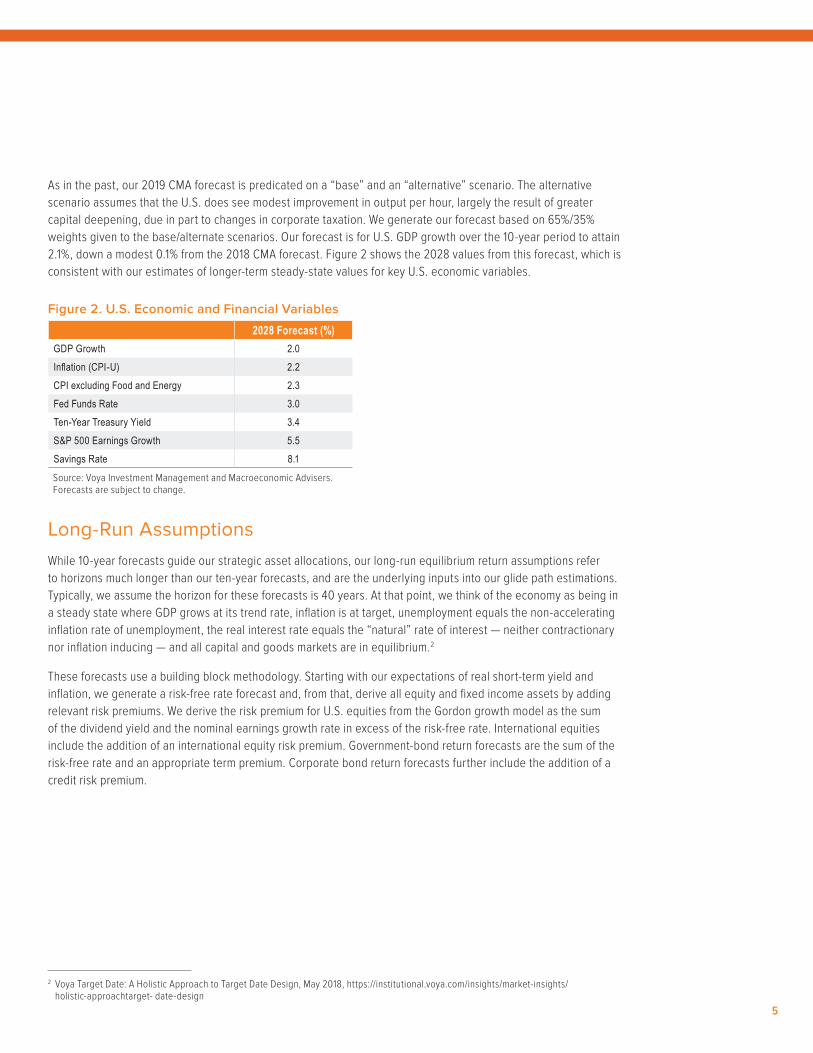
As in the past, our 2019 CMA forecast is predicated on a “base” and an “alternative” scenario. The alternative scenario assumes that the U.S. does see modest improvement in output per hour, largely the result of greater capital deepening, due in part to changes in corporate taxation. We generate our forecast based on 65%/35% weights given to the base/alternate scenarios. Our forecast is for U.S. GDP growth over the 10-year period to attain 2.1%, down a modest 0.1% from the 2018 CMA forecast. Figure 2 shows the 2028 values from this forecast, which is consistent with our estimates of longer-term steady-state values for key U.S. economic variables.

Figure 2. U.S. Economic and Financial Variables

2028 Forecast (%)GDP Growth 2.0Inflation (CPI-U) 2.2CPI excluding Food and Energy 2.3Fed Funds Rate 3.0Ten-Year Treasury Yield 3.4S&P 500 Earnings Growth 5.5Savings Rate 8.1Source: Voya Investment Management and Macroeconomic Advisers. Forecasts are subject to change.

Long-Run Assumptions While 10-year forecasts guide our strategic asset allocations, our long-run equilibrium return assumptions refer to horizons much longer than our ten-year forecasts, and are the underlying inputs into our glide path estimations. Typically, we assume the horizon for these forecasts is 40 years. At that point, we think of the economy as being in a steady state where GDP grows at its trend rate, inflation is at target, unemployment equals the non-accelerating inflation rate of unemployment, the real interest rate equals the “natural” rate of interest — neither contractionary nor inflation inducing — and all capital and goods markets are in equilibrium.2

These forecasts use a building block methodology. Starting with our expectations of real short-term yield and inflation, we generate a risk-free rate forecast and, from that, derive all equity and fixed income assets by adding relevant risk premiums. We derive the risk premium for U.S. equities from the Gordon growth model as the sum of the dividend yield and the nominal earnings growth rate in excess of the risk-free rate. International equities include the addition of an international equity risk premium. Government-bond return forecasts are the sum of the risk-free rate and an appropriate term premium. Corporate bond return forecasts further include the addition of a credit risk premium.

2 Voya Target Date: A Holistic Approach to Target Date Design, May 2018, https://institutional.voya.com/insights/market-insights/holistic-approachtarget- date-design

6

From a theoretical perspective, all risk premiums mean revert towards a long-run equilibrium as the economy is in a steady state. The reason for mean reversion is that investment opportunities are time varying. Since the rate of arrival of new information is time varying, return volatility and covariance are time varying as well in the short run. Our econometric work and that of academic researchers confirms the stationarity of a number of risk premiums, which in turn justifies our assumption of constant average risk premiums, term premiums and credit spreads in the long-run equilibrium. Our return forecasts are shown in Figure 3.

Figure 3. Long-Run Equilibrium Return Assumptions

Equilibrium Return (%)U.S. Inflation 2.0Real Risk-Free Rate 1.0U.S. Cash 3.0Aggregate Term Premium 0.9Aggregate Credit Premium 0.3U.S. Investment Grade (Aggregate) 4.210-Year Term Premium 1.210-Year U.S. Treasury 4.230-10 Year Term Premium 0.530-Year U.S. Treasury 4.7AA Corporate Credit Premium 1.2U.S. AA Corporate 5.4U.S. Equity Risk Premium 4.0S&P 500 7.0International Equity Premium 0.5MSCI ACWI 7.5Source: Voya Investment Management, as of November 2018. Assumptions are subject to change.

How We Forecast ReturnsWe derive asset-class return forecasts from the blend of the base and alternative case scenarios. Together, these capture the most important upside and downside risks which the global economy and markets will face over the forecast horizon. The base case forecasts growth to average 1.9% through 2028 driven by continued, below-trend productivity growth and subdued labor force growth. The alternative scenario assumes slightly faster productivity growth, modestly higher corporate profit share of income, a higher dividend payout ratio and an assumption that the Federal Reserve lets the economy run a little hotter than in the base case. Given these assumptions, returns to risky assets are modestly higher in the alternative scenario than in the base case.

For U.S. equities, we estimate earnings and dividends for the S&P 500 index using our blended macroeconomic assumptions. Earnings growth is constrained by the neoclassical assumption that profits as a share of GDP cannot increase without limit, but converge to a long-run equilibrium. We then use a dividend discount model to determine fair value for the index each year during the forecast period. We construct returns for other U.S. equity indices, including REITs, using a single index factor model in which beta sensitivities of each asset class with respect to the market portfolio are derived from our forward-looking covariance matrix estimation. For a detailed discussion of this, please see Covariance and Correlation Matrices Methodology, in Methodological Considerations below. Each equity asset-class return is the sum of the risk-free interest rate and a specific market-risk premium determined from our estimate of beta sensitivity and market-risk premium forecasts.

7

For U.S. bonds, we use the blended-scenario interest rate expectations to calculate expected returns for various durations. We model bond expected returns as the sum of current yield and a capital gain (or loss) based on duration and expected change in yields. For non-U.S. bonds, the process is similar and includes an adjustment for expected currency movements. Return expectations for credit-related fixed income reflect yield spreads and expected default-and-recovery rates.

Figure 4. Voya Investment Management 10-Year Returns Forecast 2019

Equity Index

Geometric Mean Return

(%)

Arithmetic Mean Return

(%)Volatility

(%) Skewness Kurtosis Sharpe RatioS&P 500 4.6 5.8 16.3 -0.48 1.0 0.18

Russell 1000 Growth 4.0 5.7 18.7 -0.44 0.7 0.15

Russell 1000 Value 5.4 6.5 15.9 -0.52 1.4 0.23

MSCI U.S. Minimum Volatility 4.9 5.5 11.6 -0.62 1.6 0.22

Russell 3000 5.0 6.3 16.8 -0.54 1.2 0.20

Russell Midcap 6.0 7.6 18.3 -0.52 1.1 0.25

Russell 2000 5.9 8.4 22.8 -0.55 1.2 0.24

MSCI EAFE 2.5 4.3 19.2 -0.28 0.2 0.08

MSCI World 4.2 5.4 16.1 -0.57 0.9 0.16

MSCI EM 4.7 8.4 27.3 -0.46 0.6 0.20

MSCI ACWI 4.4 5.8 16.9 -0.60 1.0 0.17

Expected Returns

Alternative Assets Index

Geometric Mean Return

(%)

Arithmetic Mean Return

(%)Volatility

(%) Skewness Kurtosis Sharpe RatioBloomberg Commodity 2.6 3.8 15.6 -0.41 1.5 0.06

CBOE Buy-write 4.6 5.3 12.2 -0.92 3.0 0.20

FTSE EPRA/NAREIT Developed ex U.S. 2.4 5.0 22.5 -0.17 0.6 0.10

FTSE EPRA/NAREIT Developed 3.4 5.7 21.5 -0.31 1.4 0.13

MSCI U.S. REIT 4.5 6.9 22.2 -0.35 3.0 0.18

Expected Returns

Fixed Income Index

Geometric Mean Return

(%)

Arithmetic Mean Return

(%)Volatility

(%) Skewness Kurtosis Sharpe RatioBloomberg Barclays U.S. Aggregate 2.8 3.0 7.0 0.57 4.6 0.02

Bloomberg Barclays U.S. Government Long 1.3 2.0 12.4 0.22 0.7 -0.06

Bloomberg Barclays U.S. TIPS 2.9 3.3 9.0 0.33 3.5 0.05

Bloomberg Barclays U.S. High Yield 4.5 5.2 12.1 -0.24 3.6 0.19

Credit Suisse Leveraged Loan 6.5 6.7 8.5 -0.78 15.7 0.36

Bloomberg Barclays Global Aggregate 1.2 1.5 8.6 0.35 1.8 -0.15

Bloomberg Barclays Global Aggregate ex U.S. 0.0 0.5 10.7 0.17 0.5 -0.21

JPMorgan EMBI+ 5.5 6.3 12.9 -1.65 11.5 0.24

U.S. Treasury Bill 3-Month 2.8 2.8 1.1 0.71 0.2 0.00

Source: Voya Investment Management. Returns shown are in U.S. dollar terms. Forecasts are subject to change.

8

Source: Voya Investment Management, data as of November 2018. Projections are subject to change.

Figure 5. Voya Expected Correlations Matrix

S&P

500

Russ

ell 1

000 G

rowt

h

Russ

ell 1

000 V

alue

MSC

I U.S

. Min

imum

Vol

atili

ty

Russ

ell 3

000

Russ

ell M

idca

p

Russ

ell 2

000

MSC

I EAF

E

MSC

I Wor

ld

MSC

I EM

MSC

I ACW

I

Bloo

mbe

rg C

omm

odity

CBOE

Buy

-writ

e

FTSE

EPR

A/NA

REIT

De

velo

ped

ex U

.S.

FTSE

EPR

A/NA

REIT

Dev

elop

ed

MSC

I U.S

. REI

T

Barc

lays

U.S

. Agg

rega

te

Barc

lays

U.S

. Gov

ernm

ent L

ong

Barc

lays

U.S

. TIP

S

Barc

lays

U.S

. Hig

h Yi

eld

Cred

it Su

isse

Lev

erag

ed L

oan

Barc

lays

Glo

bal A

ggre

gate

Barc

lays

Glo

bal A

ggre

gate

ex U

.S.

JPM

orga

n EM

BI+

U.S.

Trea

sury

Bill

3-M

onth

S&P 500 1.00

Russell 1000 Growth 0.96 1.00

Russell 1000 Value 0.95 0.83 1.00

MSCI U.S. Minimum Volatility 0.94 0.85 0.95 1.00

Russell 3000 1.00 0.96 0.95 0.93 1.00

Russell Midcap 0.95 0.92 0.92 0.90 0.97 1.00

Russell 2000 0.83 0.83 0.80 0.77 0.88 0.92 1.00

MSCI EAFE 0.67 0.64 0.65 0.63 0.68 0.66 0.60 1.00

MSCI World 0.93 0.90 0.89 0.87 0.93 0.91 0.81 0.90 1.00

MSCI EM 0.70 0.69 0.67 0.65 0.72 0.72 0.67 0.73 0.79 1.00

MSCI ACWI 0.92 0.89 0.88 0.86 0.92 0.90 0.81 0.89 0.99 0.85 1.00

Bloomberg Commodity 0.25 0.24 0.26 0.24 0.27 0.30 0.29 0.31 0.31 0.37 0.33 1.00

CBOE Buy-write 0.91 0.87 0.87 0.86 0.91 0.89 0.80 0.61 0.85 0.66 0.84 0.29 1.00

FTSE EPRA/NAREIT Developed ex U.S. 0.61 0.56 0.62 0.61 0.62 0.63 0.56 0.86 0.79 0.75 0.81 0.34 0.56 1.00

FTSE EPRA/NAREIT Developed 0.61 0.56 0.64 0.64 0.63 0.65 0.59 0.83 0.78 0.71 0.79 0.29 0.57 0.96 1.00

MSCI U.S. REIT 0.58 0.51 0.62 0.62 0.60 0.62 0.59 0.74 0.72 0.62 0.72 0.23 0.55 0.85 0.97 1.00

Barclays U.S. Aggregate 0.20 0.18 0.20 0.23 0.19 0.20 0.13 0.17 0.20 0.14 0.20 -0.02 0.17 0.22 0.22 0.20 1.00

Barclays U.S. Government Long 0.07 0.06 0.07 0.14 0.06 0.06 0.00 0.03 0.06 0.00 0.05 -0.10 0.05 0.10 0.11 0.12 0.89 1.00

Barclays U.S. TIPS 0.22 0.20 0.23 0.26 0.22 0.23 0.15 0.20 0.23 0.20 0.23 0.10 0.22 0.27 0.27 0.24 0.92 0.81 1.00

Barclays U.S. High Yield 0.62 0.60 0.60 0.59 0.64 0.65 0.63 0.51 0.63 0.58 0.64 0.26 0.62 0.49 0.53 0.52 0.29 0.14 0.33 1.00

Credit Suisse Leveraged Loan 0.45 0.42 0.45 0.44 0.46 0.48 0.45 0.36 0.45 0.40 0.46 0.23 0.45 0.36 0.39 0.38 0.18 0.01 0.26 0.77 1.00

Barclays Global Aggregate 0.23 0.20 0.24 0.26 0.22 0.23 0.16 0.33 0.30 0.23 0.29 0.13 0.20 0.37 0.35 0.31 0.86 0.73 0.83 0.28 0.16 1.00

Barclays Global Aggregate ex U.S. 0.22 0.19 0.24 0.25 0.22 0.22 0.16 0.37 0.31 0.25 0.31 0.18 0.19 0.40 0.38 0.32 0.71 0.59 0.71 0.25 0.13 0.97 1.00

JPMorgan EMBI+ 0.54 0.52 0.53 0.53 0.55 0.56 0.52 0.53 0.59 0.75 0.64 0.26 0.55 0.59 0.59 0.54 0.21 0.15 0.26 0.51 0.28 0.21 0.20 1.00

U.S. Treasury Bill 3-Month 0.05 0.03 0.06 0.05 0.04 0.04 0.01 0.05 0.05 0.03 0.05 0.01 0.04 0.03 0.03 0.02 0.16 0.06 0.14 0.01 0.01 0.14 0.12 0.04 1.00

9

Figure 5. Voya Expected Correlations Matrix

S&P

500

Russ

ell 1

000 G

rowt

h

Russ

ell 1

000 V

alue

MSC

I U.S

. Min

imum

Vol

atili

ty

Russ

ell 3

000

Russ

ell M

idca

p

Russ

ell 2

000

MSC

I EAF

E

MSC

I Wor

ld

MSC

I EM

MSC

I ACW

I

Bloo

mbe

rg C

omm

odity

CBOE

Buy

-writ

e

FTSE

EPR

A/NA

REIT

De

velo

ped

ex U

.S.

FTSE

EPR

A/NA

REIT

Dev

elop

ed

MSC

I U.S

. REI

T

Barc

lays

U.S

. Agg

rega

te

Barc

lays

U.S

. Gov

ernm

ent L

ong

Barc

lays

U.S

. TIP

S

Barc

lays

U.S

. Hig

h Yi

eld

Cred

it Su

isse

Lev

erag

ed L

oan

Barc

lays

Glo

bal A

ggre

gate

Barc

lays

Glo

bal A

ggre

gate

ex U

.S.

JPM

orga

n EM

BI+

U.S.

Trea

sury

Bill

3-M

onth

S&P 500 1.00

Russell 1000 Growth 0.96 1.00

Russell 1000 Value 0.95 0.83 1.00

MSCI U.S. Minimum Volatility 0.94 0.85 0.95 1.00

Russell 3000 1.00 0.96 0.95 0.93 1.00

Russell Midcap 0.95 0.92 0.92 0.90 0.97 1.00

Russell 2000 0.83 0.83 0.80 0.77 0.88 0.92 1.00

MSCI EAFE 0.67 0.64 0.65 0.63 0.68 0.66 0.60 1.00

MSCI World 0.93 0.90 0.89 0.87 0.93 0.91 0.81 0.90 1.00

MSCI EM 0.70 0.69 0.67 0.65 0.72 0.72 0.67 0.73 0.79 1.00

MSCI ACWI 0.92 0.89 0.88 0.86 0.92 0.90 0.81 0.89 0.99 0.85 1.00

Bloomberg Commodity 0.25 0.24 0.26 0.24 0.27 0.30 0.29 0.31 0.31 0.37 0.33 1.00

CBOE Buy-write 0.91 0.87 0.87 0.86 0.91 0.89 0.80 0.61 0.85 0.66 0.84 0.29 1.00

FTSE EPRA/NAREIT Developed ex U.S. 0.61 0.56 0.62 0.61 0.62 0.63 0.56 0.86 0.79 0.75 0.81 0.34 0.56 1.00

FTSE EPRA/NAREIT Developed 0.61 0.56 0.64 0.64 0.63 0.65 0.59 0.83 0.78 0.71 0.79 0.29 0.57 0.96 1.00

MSCI U.S. REIT 0.58 0.51 0.62 0.62 0.60 0.62 0.59 0.74 0.72 0.62 0.72 0.23 0.55 0.85 0.97 1.00

Barclays U.S. Aggregate 0.20 0.18 0.20 0.23 0.19 0.20 0.13 0.17 0.20 0.14 0.20 -0.02 0.17 0.22 0.22 0.20 1.00

Barclays U.S. Government Long 0.07 0.06 0.07 0.14 0.06 0.06 0.00 0.03 0.06 0.00 0.05 -0.10 0.05 0.10 0.11 0.12 0.89 1.00

Barclays U.S. TIPS 0.22 0.20 0.23 0.26 0.22 0.23 0.15 0.20 0.23 0.20 0.23 0.10 0.22 0.27 0.27 0.24 0.92 0.81 1.00

Barclays U.S. High Yield 0.62 0.60 0.60 0.59 0.64 0.65 0.63 0.51 0.63 0.58 0.64 0.26 0.62 0.49 0.53 0.52 0.29 0.14 0.33 1.00

Credit Suisse Leveraged Loan 0.45 0.42 0.45 0.44 0.46 0.48 0.45 0.36 0.45 0.40 0.46 0.23 0.45 0.36 0.39 0.38 0.18 0.01 0.26 0.77 1.00

Barclays Global Aggregate 0.23 0.20 0.24 0.26 0.22 0.23 0.16 0.33 0.30 0.23 0.29 0.13 0.20 0.37 0.35 0.31 0.86 0.73 0.83 0.28 0.16 1.00

Barclays Global Aggregate ex U.S. 0.22 0.19 0.24 0.25 0.22 0.22 0.16 0.37 0.31 0.25 0.31 0.18 0.19 0.40 0.38 0.32 0.71 0.59 0.71 0.25 0.13 0.97 1.00

JPMorgan EMBI+ 0.54 0.52 0.53 0.53 0.55 0.56 0.52 0.53 0.59 0.75 0.64 0.26 0.55 0.59 0.59 0.54 0.21 0.15 0.26 0.51 0.28 0.21 0.20 1.00

U.S. Treasury Bill 3-Month 0.05 0.03 0.06 0.05 0.04 0.04 0.01 0.05 0.05 0.03 0.05 0.01 0.04 0.03 0.03 0.02 0.16 0.06 0.14 0.01 0.01 0.14 0.12 0.04 1.00

10

Methodological Considerations

Covariance and Correlation Matrices MethodologyEstimating asset-class covariance and correlation matrices are the underlying pillars of our asset-class standard deviation forecasts. This is a different process than forecasting returns, as evidence tells us that correlations wander through time. If we were to use a historical average or exponentially weighted methodology, which takes a long-run history and puts a heavier weight on recent observations, it could lead to risk forecasts that may be representative of the past but bear little resemblance to the future. Therefore, the forecast multiple asset-class risk summarized by the return covariance matrix is crucial to the capital market assumptions process.

A simple example using equities and bonds can illustrate this point (Figure 6). Over the past 20 years, the correlation of returns between the S&P 500 index and Barclays U.S. Aggregate Bond index was -0.02; however, this tells us nothing about the relationship of returns between these two asset classes during unusual periods or when financial markets are in very euphoric or pessimistic states. For example, during normal periods of returns over the same 20-year interval, the correlation between equities and bonds was -0.10, whereas during the unusual periods it was +0.07. Incorporating these periods of unusual correlation patterns can lead to a truer estimate of the durability of diversification between asset classes. We capture these unusual periods in our standard deviation and correlation forecasts in an academic framework called turbulence.

Figure 6. Normal and Turbulent Periods of Stock and Bond Correlations, 20 Years Ended September 2018

Source: Voya Investment Management. Data as of September 2018.

Turbulence: Evolution of a Concept The turbulence framework we use to estimate correlations and standard deviations of returns among asset classes is derived from the academic work of the applied statistician Prasanta Chandra Mahalanobis. In the early twentieth century, Mahalanobis analyzed human skull resemblances among castes and tribes in India. He created a formula to capture differences in skull size, which incorporated the standard deviation of measures of various skull parts. He then squared and summed the normalized differences, generating a single composite distance measure.3

3 Mahalanobis, P., “On the Generalized Distance in Statistics,” Proceedings of the National Institute of Sciences of India vol. 2 no. 1 (1936): 49-55.

-0.10

-0.5

0.0

0.5

0.10

0.15

-0.25 -0.20 -0.15 -0.10 -0.5 0.0 0.5 0.10 0.15 0.20

Bloo

mber

g Bar

clays

U.S

. Agg

rega

te Ind

ex R

eturn

(%)

S&P 500 Index Return (%)

Tolerance RadiusNormalTurbulent

11

This formula evolved into a statistical measure called the “Mahalanobis distance.” The measure was groundbreaking in that it helped analyze data across standard deviations but also incorporated the correlations among data sets. More than 60 years later, the Mahalanobis distance was used by Kritzman and Li to formulate a concept called financial turbulence.4 They postulated financial turbulence as a condition in which asset prices, given their historical patterns of returns, behave in an uncharacteristic way including extreme price moves. They further noted that financial turbulence often coincides with excessive risk aversion, illiquidity and price declines for risky assets. It is this turbulence framework (or unusualness of returns and correlations of returns) that we have used to forecast risk measures in our capital market assumptions.

Observing TurbulenceTurbulence can be calculated for any given set of asset classes. Back to our example of U.S. equities and bonds, the two dimensions can be visualized as the equation of an ellipse using the returns of the S&P 500 index and the Bloomberg Barclays U.S. Aggregate index (Figure 6). The center of the ellipse represents the average of the joint returns of the two assets. The boundary is a level of tolerance that separates normal from turbulent observations. The boundary takes the form of an ellipse rather than a circle because it takes into account the covariance of the asset classes. The idea captured by this measure is that certain periods are considered turbulent, not only because returns are unusually high or low, but also because they move in the opposite direction of what would have been expected given average correlations.

Using Turbulence to Create Portfolios Note that the threshold of normal and turbulence in Figure 6 is not static but rather is dynamic through time. Our process identifies turbulent market regimes by estimating a covariance matrix covering those periods of market stress alone and is the outcome of a Markov model. The model classifies regimes rather than arbitrary thresholds because thresholds would fail to capture the persistence of shifts in volatility. The Markov model output in Figure 7 illustrates turbulent and normal regimes.

Figure 7. Markov Normal and Turbulent Regimes over Time

Source: Voya Investment Management. Data as of September 2018.

Turbulent market regimes make use of the concept of multivariate outliers in a return distribution. That is, we take into account not only the deviation of a particular asset class’s return from the average, but also its volatility and correlation with other asset classes. We subsequently estimate a covariance matrix based on periods of normal and turbulent market performance. Finally, we use a procedure to blend these two covariance matrices using

4 Kritzman, M. and Y. Li, “Skulls, Financial Turbulence, and Risk Management,” vol. 66 no. 5 (2010): 30‒41.

01979 1982 1985 1988 1991 1994 1997 20032000 2006 2009 2002 20182015

20

60

Markov NormalMarkov TurbulentThreshold

40

80

100

12

weights that allow us to express both views about the likelihood of each normal or turbulent regime and to capture the differential risk attitudes toward each. The weights we use are 60% normal and 40% turbulent to create our strategic asset allocation portfolios.

We overweight the turbulent regime at 40% — higher than its observed frequency of 30% — to account for structural issues such as globalization, demographics and world-wide central bank intervention, which are prevalent today. From this blended covariance matrix, we then extract the implied correlation matrix and standard deviations for each asset class. In our view, this process helps create a strategic asset allocation portfolio that can account for the empirical evidence that correlations will deviate through time.

Time Dependency of Asset Returns and Its Impact on Risk Estimation Recent research suggests that expected asset returns change over time in somewhat predictable ways and that these changes tend to persist over long periods. Thus, changes among investment opportunities — all possible combinations of risk and return — are found to be persistent. This Appendix will set out the economic reasons for return predictability, its consequences for strategic asset allocation and the adjustments we have made to control for it in our estimation process.

In our view, the common source of predictability in financial asset returns is the business cycle. The business cycle itself is persistent, and this makes real economic growth to some extent predictable. The fundamental reason for the business cycle’s persistence is that its components share the same quality. Consumers, for example, have a tendency to smooth consumption since they dislike abrupt changes in their lifestyles. Research on permanent income and lifecycle consumption provides the theoretical basis for consumers’ desire for a stable consumption path. When income is affected by transitory shocks, consumption should not change since consumers can use savings or borrowing to adjust consumption in well-functioning capital markets.

Robert Hall has formalized these ideas by showing that consumers will optimally choose to keep a stable path of consumption equal to a fraction of their present discounted value of human and financial wealth.5 Investment, the second component of GDP, is sticky, as corporate investment in projects is usually long-term in nature. Finally, government expenditures also have a low level of variability. Over a medium-term horizon, negative serial correlation sets in as the growth phase of the cycle is followed by a contraction and then that contraction is followed by renewed growth.6

How does this predictability of economic variables affect the predictability of asset returns? Consider equities as an example. The value of equities is determined as the present discounted value of future cash flows and depends on four factors: expected cash flows, expected market risk premium, expected market risk exposure and the term structure of interest rates. Cash flows and corporate earnings tend to move with the business cycle. The market risk premium is high at business cycle troughs, when consumers are trying to smooth consumption and are less willing to take risks with their income; and low at business cycle peaks, when people are more willing to take risks. The market risk premium is a component of the discount rate in the present value calculation of the dividend discount model. A firm’s risk exposure (beta), another component of the discount rate, changes through time and is a function of its capital structure. Thus, a firm’s risk increases with leverage, which is related to the business cycle. The last component of the discount rate is the risk-free rate, which is determined by the term structure of interest rates. The term structure reflects expectations of real interest rates, real economic activity and inflation, which are

5 Hall, R., “Stochastic Implications of the Life-Cycle-Permanent Income Hypothesis: Theory and Evidence,” Journal of Political Economy 86 (1978): 971–988

6 Poterba, J. and Summers, L., “Mean Reversion in Stock Prices: Evidence and Implications,” Journal of Financial Economics 22 (1988): 27–60.

13

connected to the business cycle. Thus, equity returns, and financial asset returns in general, are to a certain extent predictable. Expected returns of many assets tend to be high in bad macroeconomic times and low in good times.

This predictability of returns manifests itself statistically through autocorrelation. Autocorrelation in time series of returns describes the correlation between values of a return process at different points in time. Autocorrelation can be positive when high returns tend to be followed by high returns, implying momentum in the market. Conversely, negative autocorrelation occurs when high returns tend to be followed by low returns, implying mean reversion. In either case autocorrelation induces dependence in returns over time.

Traditional mean-variance analysis focused on short-term expected return and risk assumes returns do not exhibit time dependence and prices follow a random walk. Expected returns in a random walk are constant, exhibiting zero autocorrelation; realized short-term returns are not predictable. Volatilities and cross-correlations among assets are independent of the investment horizon. Thus, the annualized volatility estimated from monthly return data scaled by the square root of 12 should be equal to the volatility estimated from quarterly return data scaled by the square root of four. In the presence of autocorrelation, the square root of time scaling rule described above is not valid, since the sample standard deviation estimator is biased and the sign of autocorrelation matters for its impact on volatility and correlations. Positive autocorrelation leads to an underestimation of true volatility. A similar result holds for the cross-correlation matrix bias when returns exhibit autocorrelation. So for long investment horizons, the risk/return tradeoff can be very different than that for short investment horizons.

In a multi-asset portfolio, in which different asset classes display varying degrees of autocorrelation, failure to correct for the bias of volatilities and correlations will lead to suboptimal mean variance optimized portfolios in which asset classes that appear to have low volatilities receive excessive allocations. Such asset classes include hedge funds, emerging market equities and non-public market assets such as private equity or private real estate, among others.

There are at least two ways to correct for autocorrelation:

■ A direct method that adjusts the sample estimators of volatility, correlation and all higher moments

■ An indirect method that cleans the data first, allowing us to subsequently estimate the moments of the distribution using standard estimators

Given that the direct methods become quite complex beyond the first two moments, our choice is to follow the second method and clean the return data of autocorrelation. Before we do that we estimate and test the statistical significance of autocorrelation in our data series.

We estimate first-order autocorrelation correlation as the regression slope of a first-order autoregressive process. We use monthly return data for the period 1979–2014. We subsequently test the statistical significance of the estimated parameter using the Ljung-Box Q-statistic.7 The Q-statistic is a statistical test for serial correlation at any number of lags. It is distributed as a chi-square with k degrees of freedom, where k is the number of lags. Here we test for first-order serial correlation, thus k = 1. About 80% of our return series exhibit positive and statistically significant first-order serial correlation based on associated p-values at the 10% level of significance.8 Khandani and Lo provide empirical evidence that positive return autocorrelation is a measure of illiquidity exhibited among a broad set of financial assets including small-cap stocks, corporate bonds, mortgage-backed securities and

7 Ljung, G.M. and Box, G.E.P., “On a Measure of Lack of Fit in Time Series Models,” Biometrika, 65, (1978): 297–303.8 The p-value is the probability of rejecting the null hypothesis of no serial correlation when it is true (i.e., concluding that there is serial

correlation in the data when in fact serial correlation does not exist). We set critical values at 10% and thus reject the null hypothesis of no serial correlation for p-values <10%.

14

emerging market investments.9 The theoretical basis is that in a frictionless market, any predictability in asset returns can be immediately exploited, thus eliminating such predictability. While other measures of illiquidity exist, autocorrelation is the only measure that applies to both publicly and privately traded securities and requires only returns to compute.

Since the vast majority of the return series we estimate exhibits autocorrelation, we apply the Geltner unsmoothing process to all series. This process corrects the return series for first-order serial correlation by subtracting the product of the autocorrelation coefficient ρ and the previous period’s return from the current period’s return and dividing by 1-ρ. This transformation has no impact on the arithmetic return, but the geometric mean is impacted since it depends on volatility. This correction is thus important to make for long-horizon asset allocation portfolios.

New York City November 2018

Multi-Asset Strategies and Solutions TeamVoya Investment Management’s Multi-Asset Strategies and Solutions (MASS) team, led by Chief Investment Officer Paul Zemsky, manages the firm’s suite of multi-asset solutions designed to help investors achieve their long-term objectives. The team consists of 28 investment professionals who have deep expertise in asset allocation, manager selection and research, quantitative research, portfolio implementation and actuarial sciences. Within MASS, the asset allocation team, led by Barbara Reinhard, is responsible for constructing strategic asset allocations based on their long-term views. The team also employs a tactical asset allocation approach, driven by market fundamentals, valuation and sentiment, which is designed to capture market anomalies and/or reduce portfolio risk.

9 Khandani, A.E. and Lo, A., “Illiquidity Premia in Asset Returns: An Empirical Analysis of Hedge Funds, Mutual Funds, and U.S. Equity Portfolios,” Quarterly Journal of Finance 1 (2011): 205–264.

©2018 Voya Investments Distributor, LLC • 230 Park Ave, New York, NY 10169 • All rights reserved.

BSWP-CMA 120318 • IM1120-46507-1119 • 167284

Past performance does not guarantee future results.

This commentary has been prepared by Voya Investment Management for informational purposes. Nothing contained herein should be construed as (i) an offer to sell or solicitation of an offer to buy any security or (ii) a recommendation as to the advisability of investing in, purchasing or selling any security. Any opinions expressed herein reflect our judgment and are subject to change. Certain of the statements contained herein are statements of future expectations and other forward-looking statements that are based on management’s current views and assumptions and involve known and unknown risks and uncertainties that could cause actual results, performance or events to differ materially from those expressed or implied in such statements. Actual results, performance or events may differ materially from those in such statements due to, without limitation, (1) general economic conditions, (2) performance of financial markets, (3) interest rate levels, (4) increasing levels of loan defaults, (5) changes in laws and regulations, and (6) changes in the policies of governments and/or regulatory authorities.

The opinions, views and information expressed in this commentary regarding holdings are subject to change without notice. The information provided regarding holdings is not a recommendation to buy or sell any security. Fund holdings are fluid and are subject to daily change based on market conditions and other factors.

For Australian Investors

Voya Investment Management Co. LLC (“Voya”) is exempt from the requirement to hold an Australian financial services license under the Corporations Act 2001 (Cth) (“Act”) in respect of the financial services it provides in Australia. Voya is regulated by the SEC under U.S. laws, which differ from Australian laws.

This document or communication is being provided to you on the basis of your representation that you are a wholesale client (within the meaning of section 761G of the Act), and must not be provided to any other person without the written consent of Voya, which may be withheld in its absolute discretion.