20b notes: prof. daniel neuhauser - chem.ucla.edu 20b notes: prof. daniel neuhauser partially based...
TRANSCRIPT

1
20B notes: Prof. Daniel Neuhauser
Partially based on notes by Prof. Peter Felker.
Parts written by Christopher Arntsen and Arunima Coomar.
IMPORTANT: ABOUT 20% of these notes are “INSERTS”, derivations which
will not be covered in class but you’ll be expected to study and know
everything in the notes, including the inserts, for the exam.
Course overview:
This is a course about how molecules behave in aggregate – interact, form
solutions and phases, and react with useful results (heat and electricity). Along
the way we’ll learn a lot of chemistry and physics, and at times gloss over some
proofs, leaving the details to Chem. 110A (thermodynamics)
Brief outline:
1. Gases
2. Interacting systems (liquids, solids, phases)
3. Phases 4. Solutions 5. Thermodynamics: The 1st law
6. Thermodynamics: 2nd law: disorder increases in world.
7. Thermodynamics: Free energy – minimum in reactions.
8. From free energy to mass reaction law, chemical equilibrium
9. Mass reaction law and LeChatelier’s principle
10. Acids and bases; mass reaction law in acids and bases; titrations.
11. Electrochemistry
12. Kinetics
13. (Time permitting:) Raul’s law, physical properties of solutions,
colligative properties.

2
Part 1: Units and Ideal-Gases (Gas-law, Kinetics):
• Units, Avogadro’s number.
• PV=nRT – experiments, temperature scale.
• PV=nRT – theoretical proof (kinetic).
• Maxwell’s velocity distribution
• Boltzmann factor – application to vibrations.
PRELUDE (NOT COVERED IN CLASS): Review from 20A
Units, Avogadro’s numbers and moles
in practice it is difficult to deal with big # of molecules, so we measure it in
terms’ of moles. A “mol” of things means it contains
Avogadro’s’ #: NAvogadro = 6.02*1023
[We call NAvogadro interchangeably NA ]
(Note that the concept of “mol” is analogous to “dozen”; dozen molecules are 12
molecules, and a mole of molecules is 6.02*1023 molecules).
NA was adjusted to be almost exactly the number of hydrogen atoms in one gram
of hydrogen atoms. However, we have to be careful when we say that, since
hydrogen is made of separate individual H atoms only at very high temperatures
(above, say, 2000-3000 degrees).
At room temperature, hydrogen is a diatomic molecule H2; each H2 molecule
weighs twice as much as one individual hydrogen atom, so at room temperature
a mole of hydrogen molecules (H2) will weigh two grams.
(A dozen hydrogen molecules weigh twice as much as a dozen hydrogen atoms,
so a mole of hydrogen molecules weighs twice as much as a mole of hydrogen
atoms).
The mass of a hydrogen atom is almost exactly
Mass(H atom)~ 1gram/ NA = 1gram/ (6.02*1023) = 1.66*10-24 gram

3
Example: a mole of H2O will weigh about 18gram; proof:
Mass(O atom) ~ 16 Mass(H atom)
[ignoring isotopes, and other even smaller effects]
Mass(H2 molecule) = 2 Mass(H atom)
So
Mass(H2O molecule) = 18 Mass(H atoms)
So
Mass(mole H2O molecules) = 18 Mass (mole H atoms)= 18g
We therefore say
Molecular mass(H2O) = 18gram/mole
(Exercise – give the mass in gram of a single H2O molecule based on this!)
A reminder from 20A: Chemists like to change things, so they decided that the
mass of hydrogen atom will not be used as the basic definition, but rather they
say that:
1 Atomic Mass Unit (AMU) = 1/12 * mass of the 12C isotope
but those are almost the same, since
Mass(H atom) = 1.00794 * Mass (12C)/12 = 1.00794 AMU
Energy and Units
Reminder, scientists found that in nature energy (labeled by “E” or at times by
“U”) is conserved.
Energy of atoms is made of two parts. The first is the kinetic energy (K.E.),
relating to how fast each atom moves (what’s its speed, v) and what’s its mass
(m),
K.E.(one atom)= mv2/2

4
(I won’t prove this equation; you learned it or will learn in the physics series).
A side note on energy units.
Note: energy = (mass)* (speed)2 = mass *distance2 / time2
so energy is measured in units of (mass* distance2 / time2)
Energy units reminder: two sets (one called CGS and the other MKS) are
commonly used; MKS is more prevalent. The energy units get special name in
each unit system:
1 erg = 1 g cm2 / sec2 (CGS units)
1 J = 1kg m2 / sec (MKS units)
End of side note
Say that we have “N” atoms (N will be of course NAvog if we have a mole of atoms,
but we take the general case). Let’s consider the “j'th atom, i.e., we consider
either the 1st atom (in which case j=1), or the 2nd (then j=2), or the 3rd, etc.
The K.E. of the “j’th atom will be therefore
K.E.(jth atom)= mj vj2/2
So the total kinetic energy will be the sum over all “j” atoms where j will range
from “1” (the first atom) to “N” (the Nth atom) will be:
Kinetic energy for N atom: K.E. = ½ ∑ ��������,…,
(The strange symbol, Σ , means “sum”, it is the capitalized form of the Greek letter sigma; we’ll encounter more Greek letters below).
The total energy, E, has, in addition to the kinetic energy, a 2nd part called
potential energy, defined as:
Potential energy: energy that can turn to K.E.
5
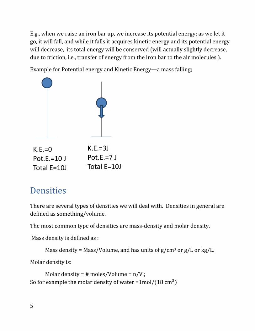
E.g., when we raise an iron bar up, we increase its potential energy; as we let it
go, it will fall, and while it falls it acquires kinetic energy and its potential energy
will decrease, its total energy will be conserved (will actually slightly decrease,
due to friction, i.e., transfer of energy from the iron bar to the air molecules ).
Example for Potential energy and Kinetic Energy—a mass falling;
Densities
There are several types of densities we will deal with. Densities in general are
defined as something/volume.
The most common type of densities are mass-density and molar density.
Mass density is defined as :
Mass density = Mass/Volume, and has units of g/cm3 or g/L or kg/L.
Molar density is:
Molar density = # moles/Volume = n/V ;
So for example the molar density of water =1mol/(18cm,)
K.E.=0
Pot.E.=10 J
Total E=10J
K.E.=3J
Pot.E.=7 J
Total E=10J
6
Pressure and Units From now on we’ll use MKS units.
To remind you: from above, energy is in units of Joule (labeled henceforth as J),
and Energy is Mass*velocity2, i.e.,
J = kg * m2/s2
But
F=Force = Energy/distance�
So
F will be measured by = J/m = (kg* m2/ s2)/m = kg* m/ s2
This force unit, J/m, has been given a special name, Newton, labeled as N
(don’t confuse this “N” with “N” the number of particles from above!)
Newton = J/m
END OF PRELUDE ON UNITS
7
Next: pressure (to be covered in class):
P=Pressure = Force/Area , and labeling the force as “F” and the area as “A”,
P = FA
P is measured in its own unit in MKS, which has been given a special name:
Pascal = Newtonm�
Multiply by m (meter) both numerator and denom.:
Pascal = Newton ∗ mm, = Jm,
(i.e., PRESSURE = ENERGY/VOLUME!)
However, 1 Newton is really a weak force in daily life (it is about the force
exerted by a quarter-pound object – e.g., a small pear – on your hand when you
hold it so it does not fall) , and a meter squared is a large area, so 1 Pascal is
actually a very weak pressure.
Ambient atmospheric pressure, i.e., pressure near sea level, is much higher than
1 Pascal
1 atmosphere ~ 1.02 * 105 Pascal.
One atmosphere is denoted as P0
It is a coincidence of nature that 1 Atmosphere is so close to a power of ten (here
100,000) times Pascal; so to use this fact, scientists introduced another pressure,
called a bar, defined as
1bar = exactly 105 Pascal
So
P0 = 1.02 bar~1bar.
A secret: since we are a little higher than sea level, the pressure at UCLA is
actually lower than P0 and is closer to a bar (and fluctuates daily with weather).
So for me, in this course, we’ll just approximate that 45" = "1789
8
and we'll ignore the 1atm vs. 1bar difference (don’t do it in other courses or labs
or you will lose points there…)
Useful: Note that
1bar = 100,000 J/m3, and m3=1000L (L means Liter),
1bar = 100,000J/(1000L)
1bar = 100 J/L
Useful later.

9
The Gas Law , Temperature scale
This section is only relevant for gases.
We'll see how experimentally the gas law, PV=nRT, was derived, where:
P: pressure V: volume T: temperature N: number of moles R: constant ("gas constant", R=8.3 J / (K mol) )
Historical route:
Separate experiments on gases by Charles and Boyle and Avogadro.
Take an amount of gas put in a piston that can move but is sealed to other gases
(see picture) so the gas inside cannot leak.
1nd : If T fixed, P*V will be proportional to the amount of material (and will be
therefore unchanged if the amount of material is unchanged, and T is fixed)
(e.g., P� P/2 when V� 2*V, but only when T and amt. of material are fixed!).
An example is in the picture below.
We have two balloons at the same temperature (say, 300K) and with the same
amount of material (say, 2mol). In one Balloon, V=25L, and the pressure is 2bar;
in the other, the volume and pressure are different (50L and 1bar), but their
product is the same as in the 1st balloon (since 25*2=50*1).
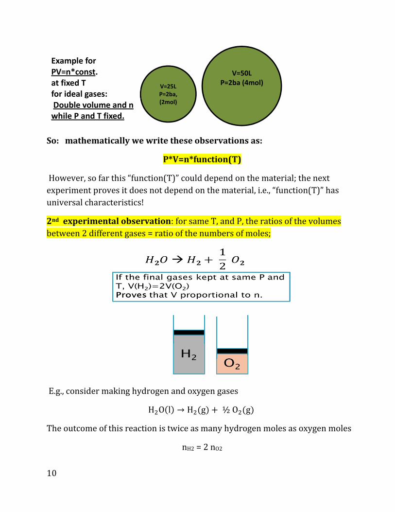
Further, if we fix T and P, and double the amount of material, then, the volume
needs to double (that’s almost obvious!), i.e., in our example:
V=50L
P=1bar
(2mol).
V=25L
P=2ba,
(2mol)
Example for
PV=n*const.
at fixed T=25oC and
fixed for ideal gases:
V doubled, P halved.
10
So: mathematically we write these observations as:
P*V=n*function(T)
However, so far this “function(T)” could depend on the material; the next
experiment proves it does not depend on the material, i.e., “function(T)” has
universal characteristics!
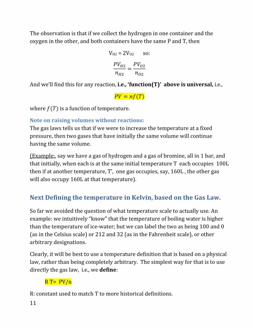
2nd experimental observation: for same T, and P, the ratios of the volumes
between 2 different gases = ratio of the numbers of moles;
E.g., consider making hydrogen and oxygen gases
H�O*l& → H�*g& = ½O�*g& The outcome of this reaction is twice as many hydrogen moles as oxygen moles
nH2 = 2 nO2
V=50L
P=2ba (4mol)
V=25L
P=2ba,
(2mol)
Example for
PV=n*const.
at fixed T
for ideal gases:
Double volume and n
while P and T fixed.
11
The observation is that if we collect the hydrogen in one container and the
oxygen in the other, and both containers have the same P and T, then
VH2 = 2VO2 so:
4?@�A@� = 4?B�AB�
And we’ll find this for any reaction, i.e., ‘function(T)’ above is universal, i.e.,
4? = AC*D& where C*D& is a function of temperature.
Note on raising volumes without reactions:
The gas laws tells us that if we were to increase the temperature at a fixed
pressure, then two gases that have initially the same volume will continue
having the same volume.
(Example:, say we have a gas of hydrogen and a gas of bromine, all in 1 bar, and
that initially, when each is at the same initial temperature T each occupies 100L
then if at another temperature, T’, one gas occupies, say, 160L , the other gas
will also occupy 160L at that temperature).
Next Defining the temperature in Kelvin, based on the Gas Law.
So far we avoided the question of what temperature scale to actually use. An
example: we intuitively “know” that the temperature of boiling water is higher
than the temperature of ice-water; but we can label the two as being 100 and 0
(as in the Celsius scale) or 212 and 32 (as in the Fahrenheit scale), or other
arbitrary designations.
Clearly, it will be best to use a temperature definition that is based on a physical
law, rather than being completely arbitrary. The simplest way for that is to use
directly the gas law, i.e., we define:
R T= PV/n
R: constant used to match T to more historical definitions.

12
The T that’s defined above is called: T in Kelvin.
The numerical value of R was adjusted so that:
The difference in Kelvin ("K") between boiling point of water and freezing point,
when measured at the pressure near sea level, will be 100 (i.e., 100K), just like it
is in Celsius.
Experimentally: put a sealed balloon filled with air in boiling water, at P=1bar,
and find that V is, say, 50.000 L. When the same balloon is then put into ice
water, we’ll find that V=36.601 L.
We find (experimentally!)
( )( )
boil
Freeze
P V at T 1bar*50.000L1.36609
P V at T 1bar*36.601L= = � BOIL BOIL
1.36609
FREEZE FREEZE
nRT T
nRT T= =
This equation is then combined with our desire to have
BOILT -T 100
FREEZEK=
To yield:
BOIL
BOIL
100 T -T 1.36609 T T 0.36609 T
i.e.,
100KT
0.36609
i.e.,
T 273.16K~273K
and
T =T +100K=373.16K
FREEZE FREEZE FREEZE FREEZE
FREEZE
FREEZE
FREEZE
K = = − =
=
=
� �
Further, we can get R from this:
Say we were able to determine that in this experiment n=1.61mol (for example,
we can weigh the air in the balloon somehow and divide by the average
molecular weight of air, including the ~80% contribution of N2, ~20% O2 , etc.).
Then:
13
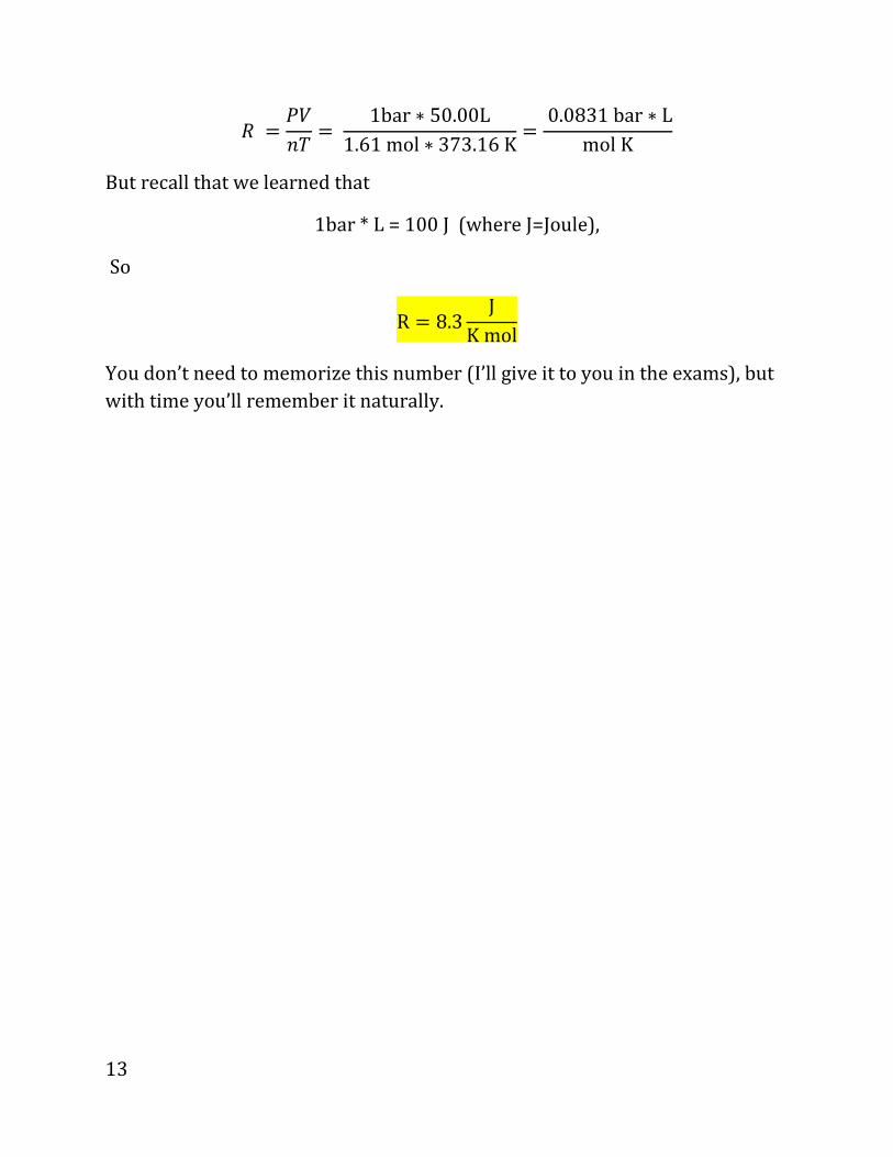
E = 4?AD = 1bar ∗ 50.00L1.61mol ∗ 373.16K = 0.0831bar ∗ LmolK
But recall that we learned that
1bar * L = 100 J (where J=Joule),
So
R = 8.3 JKmol
You don’t need to memorize this number (I’ll give it to you in the exams), but
with time you’ll remember it naturally.

14
Room temperature, and R T(room):
Officially people define, for reference, room temperature as
T(room) = 25Celisus = 298 K ;
I’ll round in this course T(room)~300K
Note: RT(room) = 8.3 J/(K mol) * 300K ~2500J/mol
WORD OF CAUTION ON THE IDEAL GAS LAW,
PV=nRT is only valid for “ideal” gases, i.e., ones in which the distances are so
large that the molecules barely meet each other once in a while. At high
pressures (e.g., bigger than say, 30bar and definitely for more than100 bar) we
have to start worrying about corrections to the ideal gas law.
But for most gases the ideal gas law is extremely accurate at room pressures.
We’ll study shortly deviations from ideal gas laws and how they teach us about
the forces that hold the atoms together in solids and liquids.
IMPORTANT: never apply the ideal gas law to liquids and solids!

15
Physical derivation of the Ideal Gas Law: kinetics
Overview
Now we’ll derive the ideal gas law; our derivation will be kinetic, i.e., based on
the properties of the motion of individual molecules. We’ll ignore on the
beigning factors of ~2.
Imagine a cubical container with a 1 mole of gas.
Assume very simplistically that:
½the molecules move to the left with a characteristic speed: u,
Another ½ move to the right with the same speed, u
(This is a very simplistic assumption, since molecules have a range of speeds;
further, they also move in different directions, not just left and right. We’ll
remedy this assumption later, one by one).
Further, our goal in this derivation is to be very simplistic, so we will sometimes
forget about factors of 2 (which will miraculously cancel out in the final relation,
i.e., our approximate derivation will give the correct result).
Before we start, several reminders:
(i) the mass density equals
�8NNOPAQRS = T?U
where n is the number of moles, M is the molar mass of the molecules, and V
is the molar volume.
(ii) momentum is defined as mass* velocity.
(iii) Force is defined as change in momentum per time
(iv) kinetic energy is defined as (up to factors of 2) mass*velocity2
16
Now to the pressure calculation: we imagine a container with unit cross
sectional area in the left wall (e.g., if we use cgs units, the area will be A=1 cm2,
etc.); the force on that area will be the pressure.
4 = V*WAXAQR89P8& But the force exerted by the molecules on the left walls the same as the force
exerted on the molecules; the latter is, as mentioned, simply the rate of change
in momentum of the molecules that hit the wall,
4 = VW9YP*XAQR89P8& = Yℎ8A[PQA�W�PARX�\
where “\" is a short time; and since the momentum equals mass*velocity, we
can write the pressure as
4= *�8NNWC]89RQY^PNRℎ8RℎQR_8^^QARQ�P\& ∗ *Yℎ8A[PQA�P^WYQRS_ℎPA�W^PY. ℎQR_8^^&\
Let’s then calculate the term.
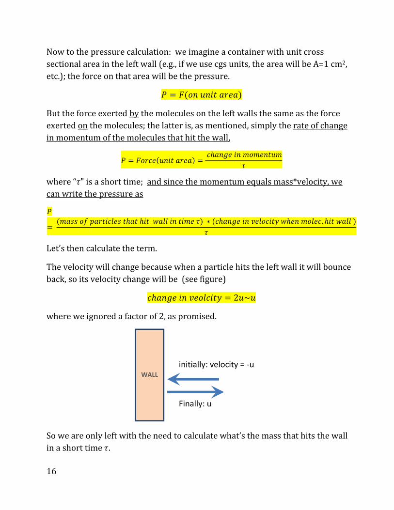
The velocity will change because when a particle hits the left wall it will bounce
back, so its velocity change will be (see figure)
Yℎ8A[PQA�PW^YQRS = 2X~X
where we ignored a factor of 2, as promised.
So we are only left with the need to calculate what’s the mass that hits the wall
in a short time \.
initially: velocity = -u
Finally: u
WALL

17
Now we know that in a time \, only particles that are within a distance X\ from
the wall can hit the wall; particles that are further way simply wont make it in
time. (See figure)
Figure: Only molecules that are within a distance bc from the wall
will hit it in time c (molecules in black, that start to the left of the
imaginary “red line” at a distance of bcfrom the wall); molecules
which are further away (blue in figure) will not hit the wall in time c.
Therefore, the volume from which particles that hit the wall come is its cross-
section area (1) times its length (u\&,i.e., it will be X\
Therefore, the mass of particles (within a unit area) that hit the wall will be the
mass density times the volume from which the particles come.
i.e.,
*�8NNWC]89RQY^PNRℎ8RℎQRRℎPXAQR − 89P8_8^^QARQ�P\& = �8NNOPANQRS ∗ *�W^X�PC9W�_ℎQYℎRℎP]89RQY^PNRℎ8RℎQRQA\899Q�P&
= T?U ∗ X\
So collecting it all we get, using the eq. we derived:
Wa
ll, A=
1
distance=uc
18
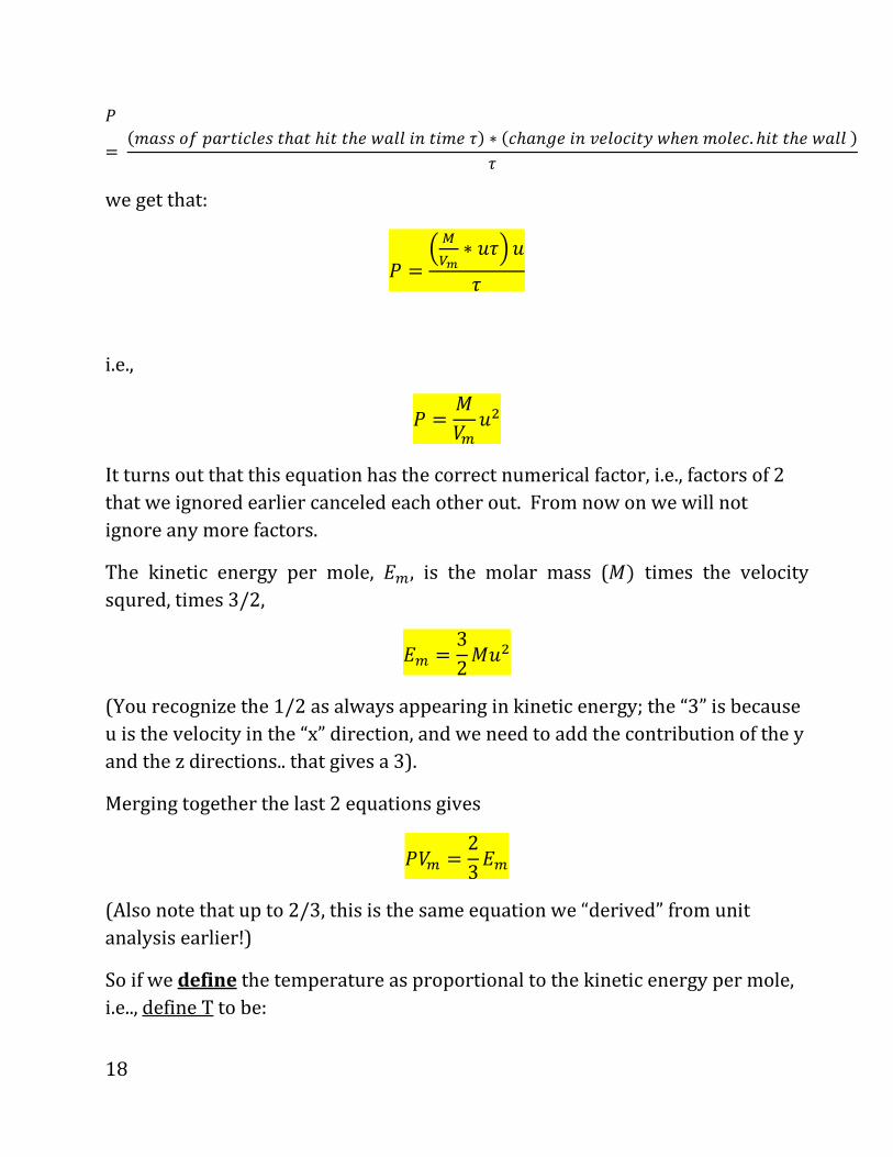
4= *�8NNWC]89RQY^PNRℎ8RℎQRRℎP_8^^QARQ�P\& ∗ *Yℎ8A[PQA�P^WYQRS_ℎPA�W^PY. ℎQRRℎP_8^^&\
we get that:
4 = efgh ∗ X\iX\
i.e.,
4 = T?U X�
It turns out that this equation has the correct numerical factor, i.e., factors of 2
that we ignored earlier canceled each other out. From now on we will not
ignore any more factors.
The kinetic energy per mole, jU, is the molar mass (T& times the velocity
squred, times 3/2,
jU = 32TX�
(You recognize the 1/2 as always appearing in kinetic energy; the “3” is because
u is the velocity in the “x” direction, and we need to add the contribution of the y
and the z directions.. that gives a 3).
Merging together the last 2 equations gives
4?U = 23jU
(Also note that up to 2/3, this is the same equation we “derived” from unit
analysis earlier!)
So if we define the temperature as proportional to the kinetic energy per mole,
i.e.., define T to be:
19
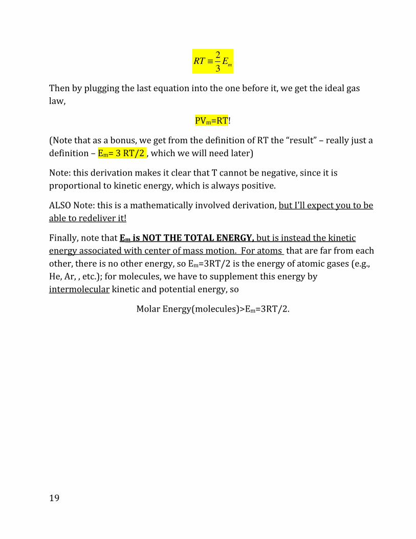
2
3mRT E≡
Then by plugging the last equation into the one before it, we get the ideal gas
law,
PVm=RT!
(Note that as a bonus, we get from the definition of RT the “result” – really just a
definition – Em= 3 RT/2 , which we will need later)
Note: this derivation makes it clear that T cannot be negative, since it is
proportional to kinetic energy, which is always positive.
ALSO Note: this is a mathematically involved derivation, but I'll expect you to be
able to redeliver it!
Finally, note that Em is NOT THE TOTAL ENERGY, but is instead the kinetic
energy associated with center of mass motion. For atoms that are far from each
other, there is no other energy, so Em=3RT/2 is the energy of atomic gases (e.g.,
He, Ar, , etc.); for molecules, we have to supplement this energy by
intermolecular kinetic and potential energy, so
Molar Energy(molecules)>Em=3RT/2.

20
Maxwell’s Velocity Distribution:
The derivation above was approximate as it assumed that all molecules have the
same speed in the x direction (with ½ going left, ½ right). Typically such
approximate derivations give results that are accurate within an order of
magnitude, i.e., have mistakes of order of 0.3 - 3.0. However, in this case we
were lucky and even the final factors were correct (so PV=nRT is correct exactly
for an ideal gas).
One issue we ignored in our derivation is that molecules do not have a fixed
speed; if we want to really know what molecules behave like, they have
distribution of speeds.
Let’s use “u” to denote the total speed. This is different from the previous
section, where u denoted the speed along x; here it denotes the total speed.
Further, u will be variable, so different molecules (or even the same molecule at
different times) will have a different u.
Since u is a continuous variable, we define the fraction of particles within a
range between u and u+du, i.e., with speeds around u but within a range du,
F*X, X = OX& = FRACTIONOF�W^PY. _QRℎX < N]PPO < X = OX
For example, a gas can have a temperature where, say, 0.03% of its molecules
have speeds between 50 and 50.1 m/s; in that case,
F(50 m/s, 50.1 m/s ) = 0.03% = 0.0003
Next, note that if du is small, F(u,u+du) is proportional to du:
F*X, X = OX& ∝ OX
(where the symbol ∝ means: proportional to).
E.g., if u is, say, 50m/s, then the number of particles that have speeds between
say 50 and 50.2 m/s will be about twice as large as the number of particles
between 50 and 50.1 m/s
21
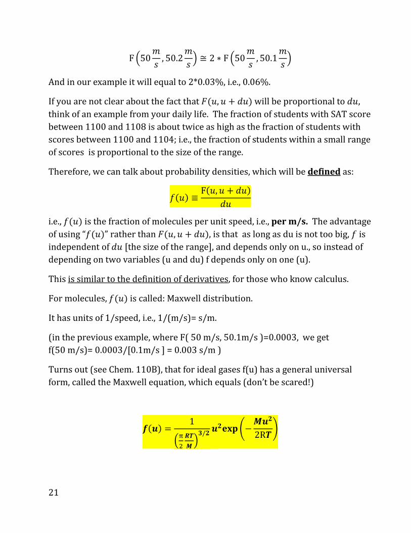
F e50�N , 50.2�N i ≅ 2 ∗ F e50�N , 50.1�N i
And in our example it will equal to 2*0.03%, i.e., 0.06%.
If you are not clear about the fact that V*X, X = OX& will be proportional to OX,
think of an example from your daily life. The fraction of students with SAT score
between 1100 and 1108 is about twice as high as the fraction of students with
scores between 1100 and 1104; i.e., the fraction of students within a small range
of scores is proportional to the size of the range.
Therefore, we can talk about probability densities, which will be defined as:
C*X& ≡ F*X, X = OX&OX
i.e.,C*X&is the fraction of molecules per unit speed, i.e., per m/s. The advantage
of using “C*X&” rather than V*X, X = OX&, is that as long as du is not too big, C is
independent of OX [the size of the range], and depends only on u., so instead of
depending on two variables (u and du) f depends only on one (u).
This is similar to the definition of derivatives, for those who know calculus.
For molecules, C*X& is called: Maxwell distribution.
It has units of 1/speed, i.e., 1/(m/s)= s/m.
(in the previous example, where F( 50 m/s, 50.1m/s )=0.0003, we get
f(50 m/s)= 0.0003/[0.1m/s ] = 0.003 s/m )
Turns out (see Chem. 110B), that for ideal gases f(u) has a general universal
form, called the Maxwell equation, which equals (don’t be scared!)
r*b& = 1es� tuv iw/x b
xyz{|−vbx2Ru}

22
M is the molar mass of the molecule, as we saw earlier.
We’ll come back later to the most important part, which is the exponential term, expe−vbx��ui; it is called the BOLTZMANN FACTOR.
Maxwell distribution Properties:
Most prevalent (m.p.) speed: where f(u) peaks.
From calculus (if you know it)
df/du=0 at um.p. �(after a short derivation)
u�.�. = �2RTM
Important alternative to calculus: deriving the probable distribution
approximately from unit analysis:
f(u)
u
e¯High T or light mass
Low T or high M: u(m.p.) lower.
X*�. ]. & = *2ED/T&12
Maxwell ‘s distribution

23
We can find out the important factor ���� in um.p. by "unit analysis”, also called
dimensional analysis, as RT
M is the only quantity with units of speed that
we can make out of RT (energy) and M (mass!)
(since velocity2=Energy/Mass, velocity=square root of (Energy/mass)).
Note that the dimensional analysis did not give us the √2 factor, but that’s
typical of dimensional analysis.
Understanding the different parts in the Maxwell distribution.
The Maxwell distribution looks very scary, but let's see that it makes sense. I'll
rewrite it as product of 4 terms
C*X& = 4√�
1XU.�., X
�exp�−�. j.RD �
Where we'll understand the terms by going right to left:
• The 4th term, expe− �.�.�� i, is the Boltzmann factor, which is, as mentioned,
very prevalent (we'll see it later): K.E. is the kinetic energy of a mole of
particles with molar mass M and speed u:
�. j.= 12TX�
So the Boltzmann factor discriminates against particles with high energies –
in this case, high kinetic energies, but later, when we talk about particles also
with potential energies, it will discriminate against other high energies (total
energies; or potential energies; depending on the circumstance).

24
• The 3rd part is an interesting part. It actually discriminates against particles
with low speeds. It turns out it is a geometric factor; which accounts for the
following:
The higher the speed, the more possibilities there are to get the same
speed u from different b�, b�, b�: i.e., if the speed is small, then that can
happen only if X� , X� and X� are all small; but if the speed is high then there
are many different combinations – X� can be high, or X� can be high, or bot
could be intermeidnate, etc.
To see a close analogy, consider what happens when we throw darts at a
circular board:
DARTS: Much higher possibility to hit the outer
rim (unless it is too far out) since it has a much larger area due
to its larger circumference.
y
X
R
25
The same argument applies for molecules, except that then we have to
replace "x" by "vx" , y by " vy", R by "u" and in 3D include also vz.
If space was 2D, the rim analysis tells us that that the geometrical factor
would have been the "circumference", which in velocity space is 2�u;
But space is 3D, so the geometrical factor is 4�u2, i.e., the surface area of a
sphere in 2D
And in general we can summarize it as : the geometrical factor is up to an
overall constant ud-1, where d is the dimensionality of our space.
• The second term in the Boltzmann distribution is the units factor
��h.�.�
This term ensures the correct units of f(u); i.e., since f(u)du is a probability,
i.e., a number with no units, f(u) has to have units of 1/speed.
Specifically, the geometrical factor has units of (speed)2 (in 3D) so the units-
factor has to be of the form of (1/speed)3, so when multiplied together, we
will get the correct (1/speed) unit for f(u)
• The left most part, �√�, is a numerical factor which ensures that overall
� C*X&OX = 1�5 , i.e., that the fraction of molecules between 0 and inifitte
speed is 100%, as it should be. This constant is the least important to
remember, and anyway it is not very far from 1 (it is ~2.5)
26
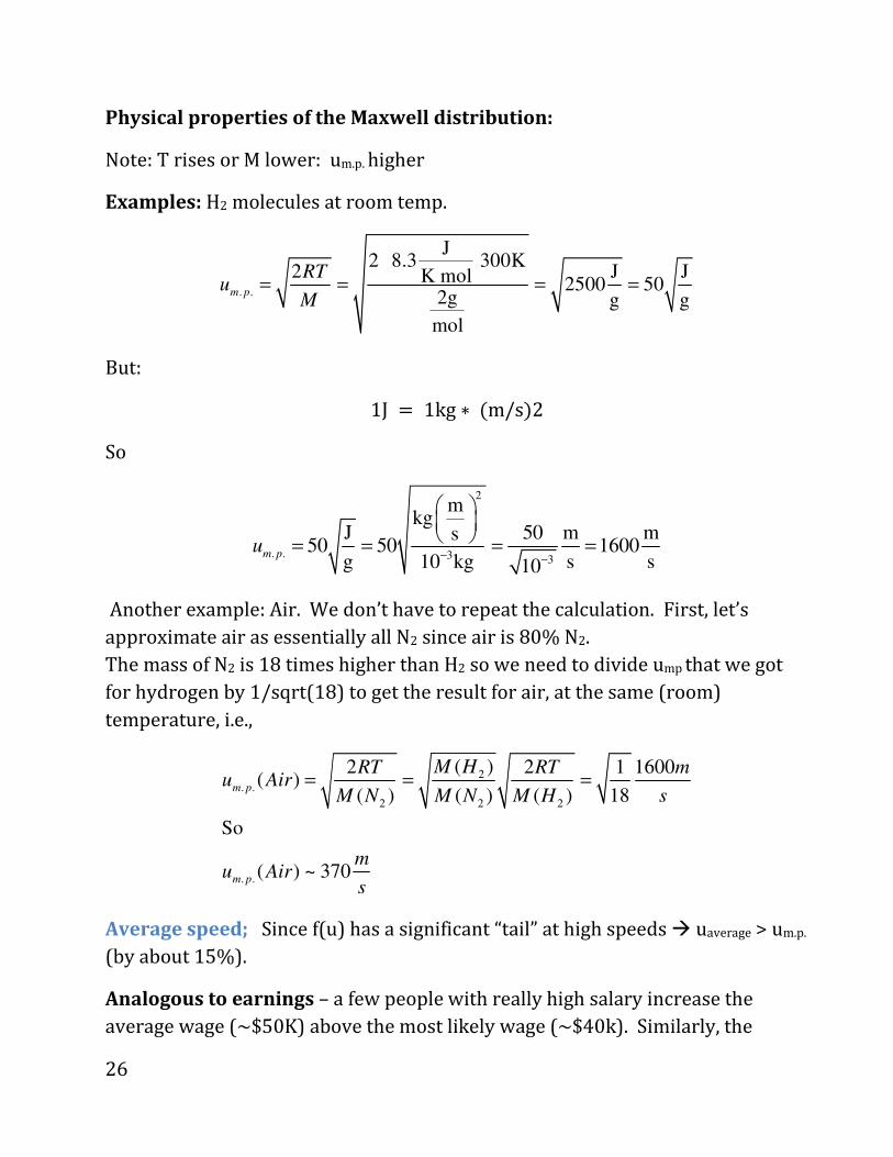
Physical properties of the Maxwell distribution:
Note: T rises or M lower: um.p. higher
Examples: H2 molecules at room temp.
. .
J2 8.3 300K
2 J JK mol 2500 502g g g
mol
m p
RTu
M= = = =
� �
But:
1J = 1kg ∗ *m/s)2So
2
. . 3 3
mkg
J 50 m ms50 50 1600
g 10 kg s s10m p
u− −
= = = =
Another example: Air. We don’t have to repeat the calculation. First, let’s
approximate air as essentially all N2 since air is 80% N2.
The mass of N2 is 18 times higher than H2 so we need to divide ump that we got
for hydrogen by 1/sqrt(18) to get the result for air, at the same (room)
temperature, i.e.,
2
. .
2 2 2
. .
( )2 2 1 1600( )
( ) ( ) ( ) 18
So
( ) ~ 370
m p
m p
M HRT RT mu Air
M N M N M H s
mu Air
s
= = =
Average speed; Since f(u) has a significant “tail” at high speeds � uaverage > um.p.
(by about 15%).
Analogous to earnings – a few people with really high salary increase the
average wage (~$50K) above the most likely wage (~$40k). Similarly, the
27
average speed is higher than the most likely speed, due to the contribution of
those very few molecules that have very high speeds.
Other implications of the average speed and the speed distribution: diffusion –
we’ll see later.
High energy tail (from Boltzmann Factor) :Explains why atmosphere does not
contain light particles (no hydrogen or helium).
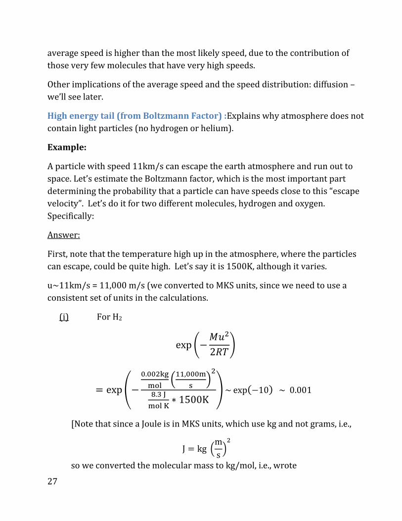
Example:
A particle with speed 11km/s can escape the earth atmosphere and run out to
space. Let’s estimate the Boltzmann factor, which is the most important part
determining the probability that a particle can have speeds close to this “escape
velocity”. Let’s do it for two different molecules, hydrogen and oxygen.
Specifically:
Answer:
First, note that the temperature high up in the atmosphere, where the particles
can escape, could be quite high. Let’s say it is 1500K, although it varies.
u~11km/s = 11,000 m/s (we converted to MKS units, since we need to use a
consistent set of units in the calculations.
(i) For H2
exp |−TX�2ED}
= exp�− 5.55�� �¡¢ e��,555�£ i�¤.,¥�¡¢¦ ∗ 1500K §~ exp*−10& ~0.001 [Note that since a Joule is in MKS units, which use kg and not grams, i.e.,
J = kg ems i�
so we converted the molecular mass to kg/mol, i.e., wrote

28
T = �W^89�8NN*¨�& = 0.002 kgmol
This conversion from g/mol to kg/mol was essential so we can cancel the
mass units in the expressions.]
Since earth exists for so long (more than 4 billion years) molecules have a
chance to reach, once in a while, the escape speed (11 km/s) and then to run
away from earth.
In contrast O2 is heavier so the Boltzmann factor is too small for anything to
escape.
Specifically, raising M by a factor of 16 (from H2 to M2 ) raises (for the same
speed), the kinetic energy by a factor of 16, so the exp e−f�©�ª�i factor, which was
before exp(-10), now becomes exp(-160)~ 10-70 , i.e., utterly negligible.
Therefore, the Boltzmann factor ensures that the probability for an oxygen
molecule to leave earth it utterly negligible, but hydrogen can leave, so our
atmosphere has lots of oxygen (and nitrogen) and little helium or hydrogen.
29
Boltzmann Factor: Consequences
As we mentioned, f�©� is a kinetic energy, labeled E, so the expoential term in
the Maxwell distribution has the form
exp|−TX�2RD} = exp �− jED�
This exponential term is very important in science and got the name “Boltzmann
Distribution” or “Boltzmann factor”.
In general, for a quantum mechanical system with different states (which are
labeled by a subscript j, then: 4(NR8RP «) = ¬ P] �− j�ED�
Where: • P stands for “probability”, don’t confuse it with P for pressure.
• C is an overall constant which will depend on temperature but not on the specific energy.
• j� is the energy of state j Note that if we have several states with the same energy, then
4(j) = ¬ ³(j)P] �− jED�
Where "N(E)" is the number of states with energy E. We encountered something similar to that when we considered the geometrical factor, u2, which essentially counts the number of "available states". A useful formulation of the Boltzmann factor which does not have the constant is when we divide the probabilities for two different energies, E and E'; then
4(j′)4(j) = ¬ ³(j′)P] e− �¸
ª�i¬ ³(j)P] e− �
ª�i = ³(j)³(j¸) exp |− j¸ − j
ED }
30
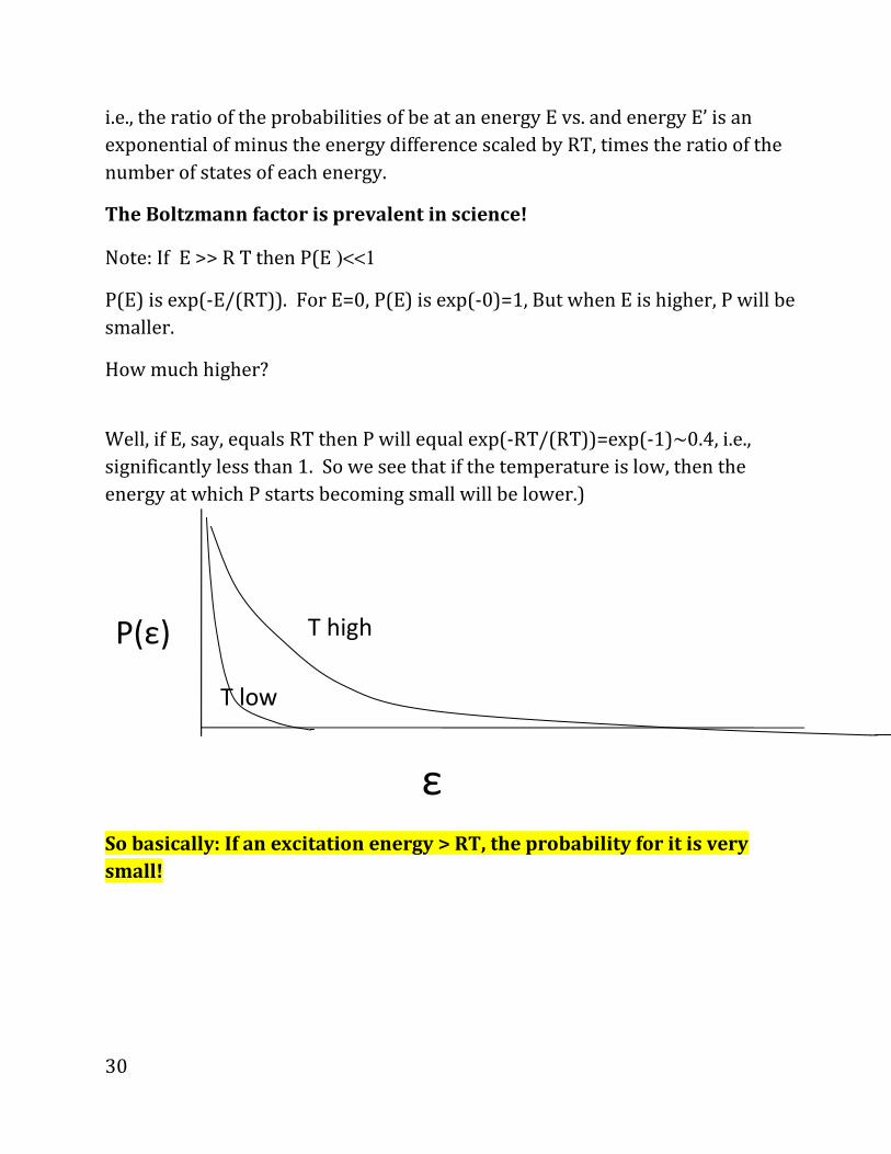
i.e., the ratio of the probabilities of be at an energy E vs. and energy E’ is an exponential of minus the energy difference scaled by RT, times the ratio of the number of states of each energy. The Boltzmann factor is prevalent in science! Note: If E >> R T then P(E )<<1
P(E) is exp(-E/(RT)). For E=0, P(E) is exp(-0)=1, But when E is higher, P will be
smaller.
How much higher?
Well, if E, say, equals RT then P will equal exp(-RT/(RT))=exp(-1)~0.4, i.e.,
significantly less than 1. So we see that if the temperature is low, then the
energy at which P starts becoming small will be lower.)
So basically: If an excitation energy > RT, the probability for it is very
small!
P(ε)
ε
T high
T low

31
Example for the Boltzmann factor: vibrations of diatoms.
Just like you learned in 20A that energy levels of electrons are discretized ,
so are vibrations;
i.e., to excite a non-vibrating molecule to vibrate even a little, you need a non-
zero amount of energy, which is
j*NQA[^P�Q798RQWA8^PYQR8RQWA& = ℎCwhere f is the vibrational frequency of the diatom, and h is Planck’s constant
(h=6.62*10-34 J s)
Since a molecule can be excited none, once, or twice, etc., the energies of the
states are (ignoring something called "zero point energy", not relevant here but
important elsewhere):
j = 0, ℎC, 2ℎC, 3ℎC, …
Further, each state has a different energy, so N(E)=1
Specific example: O2 at room temperature:
C*�Q798RQWA, ¹�& = 4.7 ∗ 10�,Hz*anIRfrequency& (recall that
1Hz=1/s)
j*1NR�Q798RQWA, ¹�& = ℎC = 6.62 ∗ 10»,�Js ∗ 4.7 ∗ 10�,*s»�& = 3.1 ∗ 10−20J
(and using 1= NAVOG /mol = 6.02*1023 /mol)
ℎC = 3.1 ∗ 10»�5J ∗ 6.02 ∗ 10�,mol
= 19 ∗ 10,J
mol = 19 kJmol
Also, for room temperature
ED = 8.3 JmolK ∗ 300K~2500 J
mol = 2.5 kJmol :
32
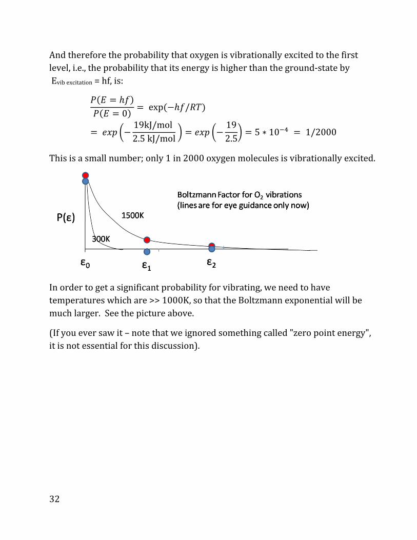
And therefore the probability that oxygen is vibrationally excited to the first
level, i.e., the probability that its energy is higher than the ground-state by
Evib excitation = hf, is:
4*j = ℎC&4*j = 0) = exp*dZC/ED&. P] �d 19kJ/mol2.5kJ/mol� . P] �d 192.5� . 5 ∗ 10»� . 1/2000
This is a small number; only 1 in 2000 oxygen molecules is vibrationally excited.
In order to get a significant probability for vibrating, we need to have
temperatures which are >> 1000K, so that the Boltzmann exponential will be
much larger. See the picture above.
(If you ever saw it – note that we ignored something called "zero point energy",
it is not essential for this discussion).

33
INSERT (read at home, required material)
Another example for the Boltzmann factor:
Barometric pressure dropoff with height
There are several ways to determine the falloff of the air pressure above earth
with height; for our purposes, it is interesting to see that we can get it from stat.
mech.
The potential energy of a molecule above earth is
½*Z& . T[̅Z Where h is the height, M is the molar mass, and [̅ is the gravitational constant
([̅ . 9.8 ¿ÀÁ¡ã� . 9.8 ¥� �, since Newton = ¥� .) Also, I use a "bar" so we don’t
confuse [̅ with g for gram )
The "state" of the molecule is its height, h; further, it turns up that the N(E)
factor is constant in this case.
Therefore, the Boltzmann distribution tells us then that the ratio of the
probability of having a molecule near a height "h" compared with another
height, say, "0", is
4�ÄÅÆ*Z&4�ÄÅÆ*0& = exp |− T[̅*ℎ − 0&ED } = exp �− T[̅ℎED �
The ratio of probabilities is, quite intuitively, the same as the ratio of molar
densities at height h vs. sea level,
A*Z&A*0& = 4�ÄÅÆ*ℎ&4�ÄÅÆ*0&
; but since the molar density is proportional to the pressure, the equation above
also is the same as the ratio of pressures; i.e., we can interpret the equation
above as if "P" is also the pressure, i.e.,

34
4�ÄÇÈÈ�ÄÇ*Z&4�ÄÇÈÈ�ÄÇ*0& = A*ℎ&A*0& = 4�ÄÅÆ*ℎ&4�ÄÅÆ*0& = exp �− T[̅ℎED �
(this is the only place in the course where it is allowed to confuse "P” for
probability with "P" for pressure!)
If you plug in the numbers you see that, for example for oxygen (O2,
M~32g/mol), when h=2km=2000m, and T=300K (so RT=2500J/mol) then
4*Z . 2000m&4*0& = exp �− T[̅ℎED � = exp �− ,� �¡¢ ⋅ 9.8 ¥� � ⋅ 2000m�Ê55¥�¡¢
§= exp �−251 gkg� ~ exp*−0.25& = 0.78
i.e., at 2km above sea level (about 6600 ft. above sea level, so above Denver but
below Mexico City), the pressure is about 0.78 atmosphere.
END OF INSERT

35
Part 2: Real Gases, Solids, Liquids
Overview:
• Gas and Liquid volumes, distances
• Attraction and repulsions, Z=PV/nRT,
• Potential energy of interactions.
• Physical Properties: compressibility, thermal expansion coeff., discussion,
surface tension
• Intermolecular forces: Columbic and dipole:
Ion-dipole, dipole-dipole, induced forces, fluctuation-induced (vdW) forces,
exchange-repulsion.
• Boiling points and hydrogen bonds
Gas Volume
Gas volumes—practical numbers
For T(room) and Po , the volume of one mole, labeled molar volume, Vm is:
V� . RTP . 8.3JKmol ∗ 300�100 ¥Ì. 25 Lmol
i.e., One mole of ideal gas occupies 25L at room pressure and temperature.
Distance between gas molecules--estimate:
Let’s estimate the distance between each molecule.
For this, let’s first in our mind (i.e., doing a “thought experiment”) take a mole of
molecules in a gas, and do a snap shot of all the molecules in that volume at a
single instant of time. Then, divide space to imaginary cells, such that each cell
contains exactly one molecule.
36
Now some of these cells will be very small, as will happen if a molecule happens
to be close to a few others; a cell could also be big, if the molecule it contains
happens to be far from the other molecules.
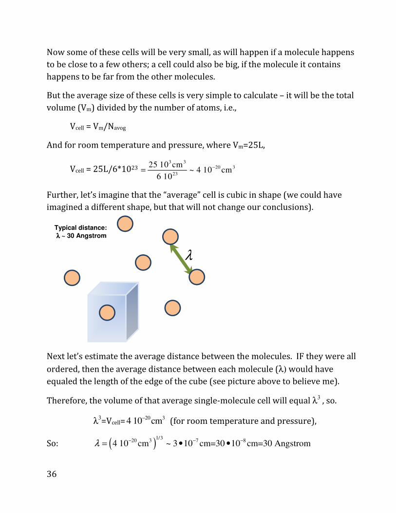
But the average size of these cells is very simple to calculate – it will be the total
volume (Vm) divided by the number of atoms, i.e.,
Vcell = Vm/Navog
And for room temperature and pressure, where Vm=25L,
Vcell = 25L/6*1023 3 3
20 3
23
25 10 cm~ 4 10 cm
6 10
−=�
��
Further, let’s imagine that the “average” cell is cubic in shape (we could have
imagined a different shape, but that will not change our conclusions).
Next let’s estimate the average distance between the molecules. IF they were all
ordered, then the average distance between each molecule (λ) would have
equaled the length of the edge of the cube (see picture above to believe me).
Therefore, the volume of that average single-molecule cell will equal λ3 , so.
λ3=Vcell=20 34 10 cm−
� (for room temperature and pressure),
So: ( )1/3
20 3 7 84 10 cm ~ 3 10 cm=30 10 cm=30 Angstromλ − − −= • •�
λ
Typical distance:
λ λ λ λ ~ 30 Angstrom
37
(recall that 1Angstrom is defined as 10-8 cm)
Liquid volumes:
Unlike ideal gases, liquid volumes are dependent on the material;
Also, in general liquids are much denser than gases.
Let’s see an example: molar volume of liquid water; this example will then allow
us to estimate the volume of each water molecule.
We know one mole of liquid water weights 18 g, and its mass density
(mass/volume) is
mass density (liquid H2O) = 1g/cm3
(that is of course not a coincidence but was used to define the gram when the
meter was adopted by French scientists more than 200 years ago),
So
Volume(one mole liquid H2O)
=(mass of one mole)/ (mass/volume)
= (mass of one mole)/density
Now, the molar mass of water, as we saw is 18g/mol;
so the mass of one mol=18(g/mol)*1mol = 18g,
And further, the density of water is 1g/cm3, so
Volume(one mole liquid H2O) = 18g/(1g/cm3) = 18cm3 =18*10-3L
Compare this number to gases, which at one bar and room temperature have a
molar volume of 25L!
i.e., Liquid water is more than 1000 times denser than ideal gases at room
temperature and pressure!
38
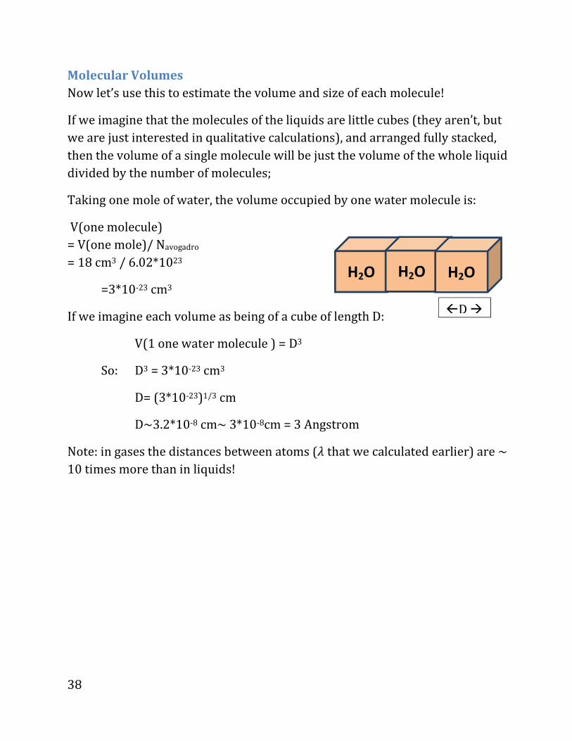
Molecular Volumes
Now let’s use this to estimate the volume and size of each molecule!
If we imagine that the molecules of the liquids are little cubes (they aren’t, but
we are just interested in qualitative calculations), and arranged fully stacked,
then the volume of a single molecule will be just the volume of the whole liquid
divided by the number of molecules;
Taking one mole of water, the volume occupied by one water molecule is:
V(one molecule)
= V(one mole)/ Navogadro
= 18 cm3 / 6.02*1023
=3*10-23 cm3
If we imagine each volume as being of a cube of length D:
V(1 one water molecule ) = D3
So: D3 = 3*10-23 cm3
D= (3*10-23)1/3 cm
D~3.2*10-8 cm~ 3*10-8cm = 3 Angstrom
Note: in gases the distances between atoms (Í that we calculated earlier) are ~
10 times more than in liquids!
H2O H2O H2O
�D �
39
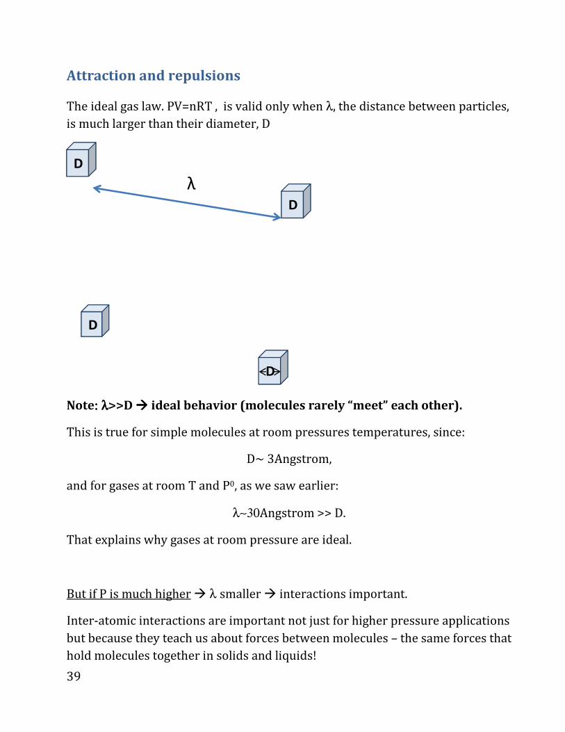
Attraction and repulsions
The ideal gas law. PV=nRT , is valid only when λ, the distance between particles,
is much larger than their diameter, D
Note: : : : λλλλ>>D ���� ideal behavior (molecules rarely “meet” each other).
This is true for simple molecules at room pressures temperatures, since:
D~ 3Angstrom,
and for gases at room T and P0, as we saw earlier:
λ∼30Angstrom >> D.
That explains why gases at room pressure are ideal.
But if P is much higher � λ smaller � interactions important.
Inter-atomic interactions are important not just for higher pressure applications
but because they teach us about forces between molecules – the same forces that
hold molecules together in solids and liquids!
D
D
D
D
λ
40
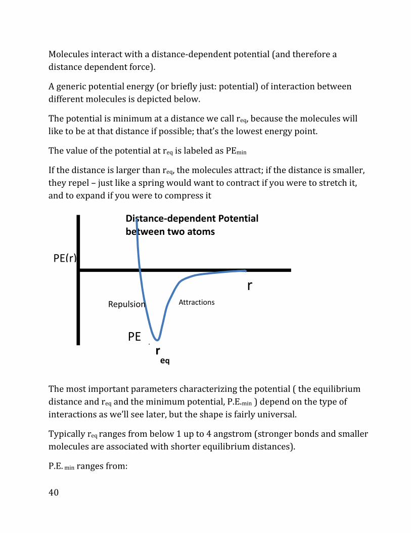
Molecules interact with a distance-dependent potential (and therefore a
distance dependent force).
A generic potential energy (or briefly just: potential) of interaction between
different molecules is depicted below.
The potential is minimum at a distance we call req, because the molecules will
like to be at that distance if possible; that’s the lowest energy point.
The value of the potential at req is labeled as PEmin
If the distance is larger than req, the molecules attract; if the distance is smaller,
they repel – just like a spring would want to contract if you were to stretch it,
and to expand if you were to compress it
The most important parameters characterizing the potential ( the equilibrium
distance and req and the minimum potential, P.E.min ) depend on the type of
interactions as we’ll see later, but the shape is fairly universal.
Typically req ranges from below 1 up to 4 angstrom (stronger bonds and smaller
molecules are associated with shorter equilibrium distances).
P.E. min ranges from:
PE(r)
r
Distance-dependent Potential
between two atoms
req
PEmi
Attractions Repulsion

41
9eV (about 900 kJ/mole) for N2
to 0.002eV or lower for weakly interacting helium atoms.
In general:
At far away distances (typically above 2req , i.e., at above 5-8 Angstrom) , the
particles barely interact.
What happens at closer distances? Recall that particles will like to get to regions
with low potential (nature loves “negative energy”, i.e., lowering the potential.)
So for req<r the particles will like to get together, to lower their distance to req,
therefore they attract;
For r<req they strongly repel (particles cannot interpenetrate too much).
Therefore: if the pressure is increased but not too large (typically tens and
hundreds of bars), particles get closer to each other, attract each other, and since
they “like each other”, the volume will fall below the ideal gas law prediction.
When the pressures are very high (hundreds or thousands of bars and more)
particles push each other away, so the volume is increased beyond what the
ideal gas law predicts.
42
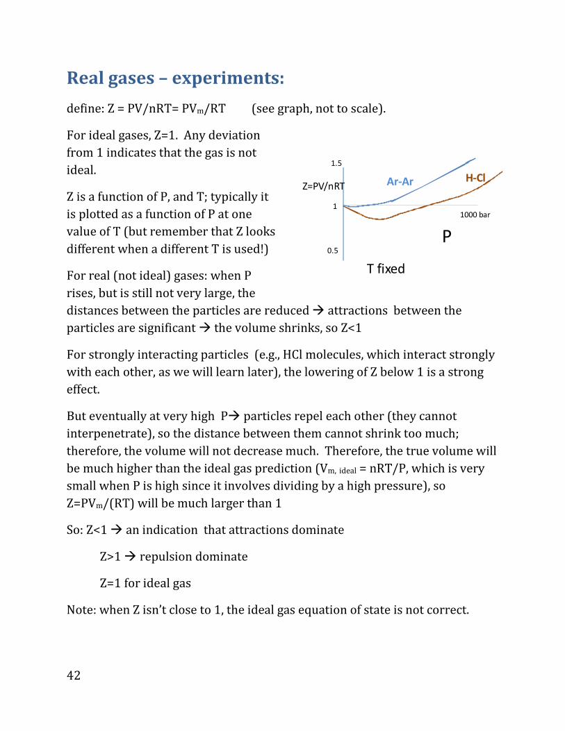
Real gases – experiments:
define: Z = PV/nRT= PVm/RT (see graph, not to scale).
For ideal gases, Z=1. Any deviation
from 1 indicates that the gas is not
ideal.
Z is a function of P, and T; typically it
is plotted as a function of P at one
value of T (but remember that Z looks
different when a different T is used!)
For real (not ideal) gases: when P
rises, but is still not very large, the
distances between the particles are reduced � attractions between the
particles are significant � the volume shrinks, so Z<1
For strongly interacting particles (e.g., HCl molecules, which interact strongly
with each other, as we will learn later), the lowering of Z below 1 is a strong
effect.
But eventually at very high P� particles repel each other (they cannot
interpenetrate), so the distance between them cannot shrink too much;
therefore, the volume will not decrease much. Therefore, the true volume will
be much higher than the ideal gas prediction (Vm, ideal = nRT/P, which is very
small when P is high since it involves dividing by a high pressure), so
Z=PVm/(RT) will be much larger than 1
So: Z<1 � an indication that attractions dominate
Z>1 � repulsion dominate
Z=1 for ideal gas
Note: when Z isn’t close to 1, the ideal gas equation of state is not correct.
Z=PV/nRT
P
Ar-Ar H-Cl
1
0.5
1.5
1000 bar
T fixed
43
Solids, Liquids, gases: physical properties.
Solids and liquids: packed together, together labeled as “condensed phases”
Forces: balanced repulsion + attraction.
We saw: equilibrium distances 2-5 Angstroms;
Distances in gases we saw ~ 30 Angstroms.
Compressibility
κ (kappa) = fractional change in volume per pressure change, when T is fixed.
Gases:
In an ideal gas, κ is large 1
For example if the initial gas pressure is 1bar, and at fixed T we reduce the
pressure by 1%to 0.99bar, then, since PV will be fixed (PV=nRT which does not
change), V will increase by about 1%
So κ for a gas (at P0) = (fractional change of volume)/ (pressure change) ~
1%/0.01atm =1/atm.
i.e., κ(gases) = 1/P = 1/atm (for standard conditions, P=1 atm)
But for Solids and Liquids
κ(solid/liq.)~ 10-4/atm, much smaller than for gases;
Example: in a diving pool, for each 1 meter we lower ourselves, the pressure on
us rises by about 0.1 bar; but our volume barely changes even when we dive!
1 we say ideal gas, but remember that for pressures that are typically encountered in a lab, below 10 bar, real gases are essentially ideal, so below we will refer to real gases as if they were ideal and just call them all gases; of course, as you saw in the discussion of Z, at high pressures the real vs. ideal gases distinction is very important.
44
Reason that κ(solid/liq.) is small : In liquids and solids, the positions are
generally near the equilibrium distances; we need very large pressures for r to
decrease significantly from r=req to lower value.
Thermal expansion
The thermal expansion coefficient measures the percent change in volume when
we raise the temperature:
α (alpha) = fractional change in volume / temperature change
For gases: α is big, since V is proportional to T;
? . AED4
So, if P is fixed, then if we change the temperature by 1% then the volume will
change by 1%, i.e., a big change.
But for condensed phases(i.e., solids or liquids) this isn’t true; α is much
smaller.
E.g., when the temperature changes by 3% (9 degrees Celsius, around 16
Fahrenheit) a car does not change its volume much.
The thermal expansion coefficient for solids and liquids is about 1/1000 times
lower than for gases, just like the compressibility.
45
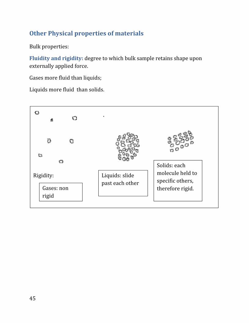
Other Physical properties of materials
Bulk properties:
Fluidity and rigidity: degree to which bulk sample retains shape upon
externally applied force.
Gases more fluid than liquids;
Liquids more fluid than solids.
Rigidity:
Solids: each
molecule held to
specific others,
therefore rigid. Gases: non
rigid
Liquids: slide
past each other
46
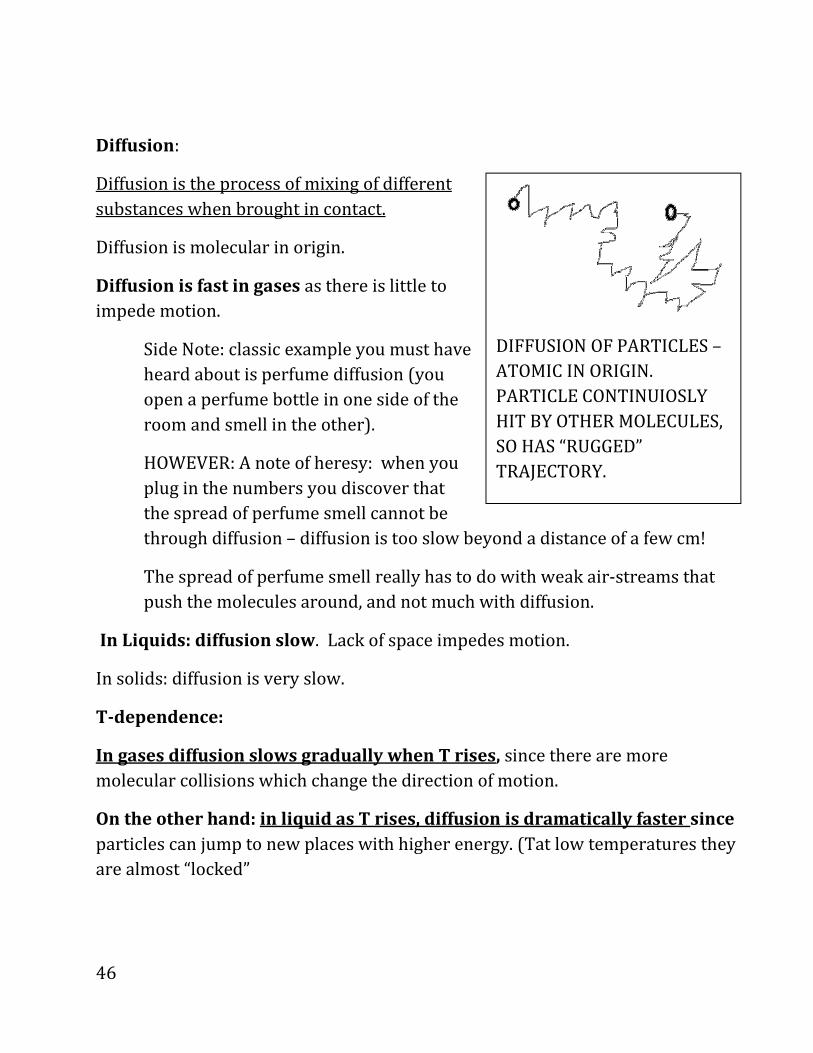
Diffusion:
Diffusion is the process of mixing of different
substances when brought in contact.
Diffusion is molecular in origin.
Diffusion is fast in gases as there is little to
impede motion.
Side Note: classic example you must have
heard about is perfume diffusion (you
open a perfume bottle in one side of the
room and smell in the other).
HOWEVER: A note of heresy: when you
plug in the numbers you discover that
the spread of perfume smell cannot be
through diffusion – diffusion is too slow beyond a distance of a few cm!
The spread of perfume smell really has to do with weak air-streams that
push the molecules around, and not much with diffusion.
In Liquids: diffusion slow. Lack of space impedes motion.
In solids: diffusion is very slow.
T-dependence:
In gases diffusion slows gradually when T rises, since there are more
molecular collisions which change the direction of motion.
On the other hand: in liquid as T rises, diffusion is dramatically faster since
particles can jump to new places with higher energy. (Tat low temperatures they
are almost “locked”
DIFFUSION OF PARTICLES –
ATOMIC IN ORIGIN.
PARTICLE CONTINUIOSLY
HIT BY OTHER MOLECULES,
SO HAS “RUGGED”
TRAJECTORY.

47
Biology relevance: In small living cells (with size below about 1 micron)
diffusion is a mechanism for transport; in bigger or more developed cells other
mechanisms (transport along “chains”) dominate.
Surface Tension:
Molecules in liquids love to have several neighbors (we’ll learn the details of the
molecular interactions in a few pages).
But molecules on the surface of liquids cannot interact with many neighbors (for
example, in water-air interface, a water molecule on the surface does not have
molecules above it, except for an occasional air (N2) molecule arriving rarely).
Therefore � liquids try to minimize
their liquid-air (or generally liquid-
gas) surface area, to have as few
molecules on the surface as possible.
The strength of this “surface tension”
effect depends on the type of the
liquid.
Weakly interacting liquids (e.g., He-
Ar, Ar-Ar at very low temperatures, where they are liquids) have weaker surface
tension, i.e., they “do not mind” having a large surface.
Note: sometimes (e.g., water near wood) the interactions with another surface
are actually quite favorable, e.g.., a water molecule likes the surface of some
other materials even more than it likes other water molecules. This leads to the
opposite of surface tension, a phenomena which is called capillary action:
Capillary action leads to the rise of liquid in a narrow
confine (the water climbs to “wet” more of the surface
area of the wood)� capillary action is responsible for
delivery of water to and within leaves (water rises
within the leaves against the force of the gravity).
Figure: Minimization of surface area
(“surface tension”) causes
coalescences of liquid drops to
minimize area; causes liquid drops to
resist breaking down

48
Intermolecular forces: Columbic and dipole
Inter means “between different things”. Intermolecular forces are the forces
between different molecules; this is the opposite of intramolecular forces, which
are the forces within a molecule.
Intermolecular forces control chemical and biological behavior, since they are
weaker than chemical bonds (i.e., weaker than intramolecular forces, which are
so strong that bonds are usually fixed; so it is almost paradoxical that the
strongest bonds are not that important biologically—as they don’t change!).
Intermolecular forces are mostly electronic (due to attractions between
different charges), and are caused less by quantum mechanics (QM) (except for
some aspects of van-der-Waals forces, as we’ll see later).
Contrast this with the important role that QM plays in covalent bonds.
Inter- vs. Intra- molecular forces comparison:
Intermolecular interactions: typically 1-50 kJ/mol
vs. Intramolecular forces (covalent, ionic): 200-900 kJ/mol.
Side note: Contrast this with RT~2.5kJ/mol;
So we see that the intermolecular interactions are not much larger
than RT, which is a measure of the thermal energy;
But RT<< strength of intramolecular forces, so temperature barely
affects strength of intra molecular bonds..
Intermolecular forces: slower fall-off, Intermolecular forces: less directed:
Little energy to rotate
around molecules
But :Within a molecule (intra-
): a lot of energy to rotate
bond
49
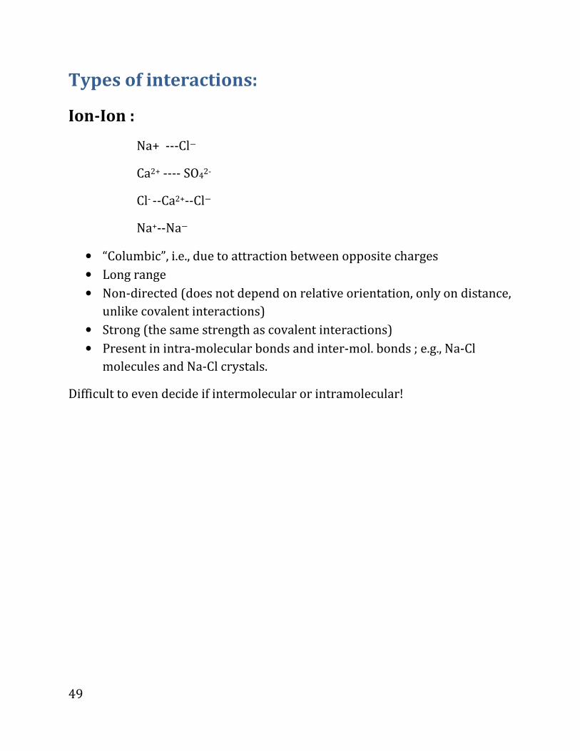
Types of interactions:
Ion-Ion :
Na+ ---Cld
Ca2+ ---- SO42-
Cl- --Ca2+--Cld
Na+--Nad
• “Columbic”, i.e., due to attraction between opposite charges
• Long range
• Non-directed (does not depend on relative orientation, only on distance,
unlike covalent interactions)
• Strong (the same strength as covalent interactions)
• Present in intra-molecular bonds and inter-mol. bonds ; e.g., Na-Cl
molecules and Na-Cl crystals.
Difficult to even decide if intermolecular or intramolecular!
50
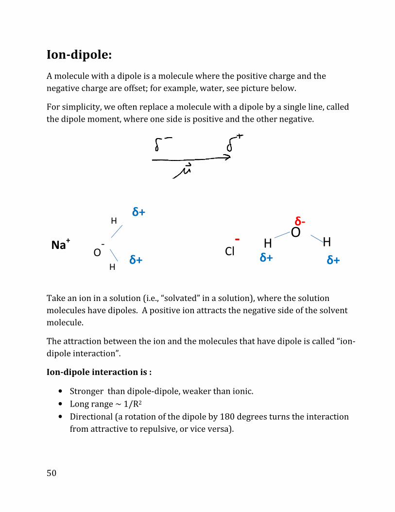
Ion-dipole:
A molecule with a dipole is a molecule where the positive charge and the
negative charge are offset; for example, water, see picture below.
For simplicity, we often replace a molecule with a dipole by a single line, called
the dipole moment, where one side is positive and the other negative.
Take an ion in a solution (i.e., “solvated” in a solution), where the solution
molecules have dipoles. A positive ion attracts the negative side of the solvent
molecule.
The attraction between the ion and the molecules that have dipole is called “ion-
dipole interaction”.
Ion-dipole interaction is :
• Stronger than dipole-dipole, weaker than ionic.
• Long range ~ 1/R2
• Directional (a rotation of the dipole by 180 degrees turns the interaction
from attractive to repulsive, or vice versa).
O
δ-
H
δ+
H
δ+
Cl-
O-
H
δ+
H
δ+
Na+
51
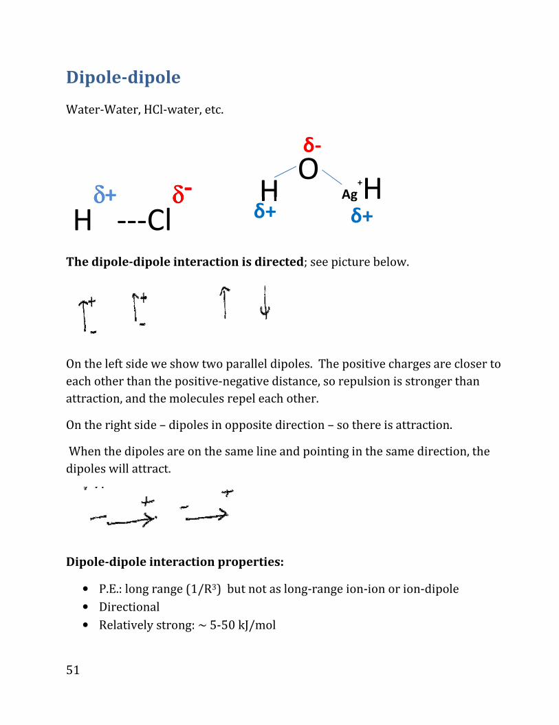
Dipole-dipole
Water-Water, HCl-water, etc.
The dipole-dipole interaction is directed; see picture below.
On the left side we show two parallel dipoles. The positive charges are closer to
each other than the positive-negative distance, so repulsion is stronger than
attraction, and the molecules repel each other.
On the right side – dipoles in opposite direction – so there is attraction.
When the dipoles are on the same line and pointing in the same direction, the
dipoles will attract.
Dipole-dipole interaction properties:
• P.E.: long range (1/R3) but not as long-range ion-ion or ion-dipole
• Directional
• Relatively strong: ~ 5-50 kJ/mol
Hδδδδ+
---Clδδδδ-
O
δ-
H
δ+
Ag+H
δ+
52
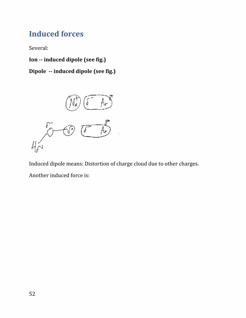
Induced forces
Several:
Ion -- induced dipole (see fig.)
Dipole -- induced dipole (see fig.)
Induced dipole means: Distortion of charge cloud due to other charges.
Another induced force is:

53
Induced dipole-induced dipole; (Van-der-Walls potential)
Imagine, e.g., Ar-Ar.
QM says there are fluctuations, i.e., times when the electrons are not in a
spherically symmetric shape. For example, there will be times when the
fluctuation will look like this (electrons move to right):
Each fluctuation will induce a dipole in the other molecule, e.g.:
Alternately, a fluctuation along the “y” axis in one atom will induce a dipole in
the –y direction in the other atom:
Ar
Ar
Ar δ+ δ-
Fluctuation
Ar
Ar
δ+ δ- Ar
δ+ δ-
Ar
δ
δ-
Ar
δ
δ-
54
Properties of the vdW (van-der-Waals) interaction:
• Always attractive., so it is not very directional (i.e., even for molecules, the
interaction does not depend much on the relative orientation of the
molecule). Contrast this with the interaction between two molecules with
permanent dipoles, which will attract or repel each other depending on
direction. • Very short-range, 1/R6
• Since always attractive, adds up. Can be significant for large surfaces –
causes two regions with large surface area that are placed near each other
to stick together.
55
Finally we get from attraction (or mild repulsion) to strong repulsions when
atoms get too close:
Exchange Interaction: Repulsive
Due to Pauli principle – not more than 2 electrons can be in the same orbitals.
When we bring two molecules together, the orbitals of each atom start
overlapping the core orbitals of the other atoms;
There is no space in these core orbitals for more electrons (they are filled up
already), so, due to the Pauli principle, the electrons from the other atom need to
be bumped up in energy to high energy orbitals,.
That increases the energy, and higher energy is less “desirable”, i.e., the potential
energy increases so that there is repulsion
Higher energy � repulsion..
Exchange interaction is VERY SHORT RANGE. It is modeled as if it is a strongly
increasing function when R is smaller; typically, it is modeled as proportional to
1/R12 (note that we decrease the distance by a factor of, 1/R12 increases by a
factor of 212, i.e., by a factor of 4000!).

56
Manifestation of Inter-Molecular forces: Boiling
Points, Hydrogen bonds.
As T rises, K.E. (kinetic energy)rises.
When T rises, the higher K.E. eventually overwhelms the attraction; so the avg.
molecule has enough K.E. to escape from its neighboring molecules,
I.e. if the initial material is a liquid then as T rises, eventually the molecules will
have enough kinetic energy to run away, and then the material “boils”, i.e.,
converts to gas..
Therefore:
Larger attractive forces � need higher K.E. to escape � Boiling T (TB ) higher.
Examples:
• The strongest bonds: ionic materials
TB(NaCl) = 1686 K ion-ion interactions, very strong).
• The weakest bonds: small molecules interacting by vdW forces
TB(N2) ~ 77K,
TB(He)~4K
Both are low temperatures since nitrogen and helium interact through very
weak vdW potentials (i.e., vdW liquids –an abbreviation for liquids interacting
mainly by vdW forces --- have low boiling temperatures unless the molecules
are really big). The boiling temperature is much lower for helium since it has
much less “fluctuation”, i.e., its electrons are held tightly and are not
“polarizable”.
Contrast this with the higher boiling temperatures of some hydrides:
TB(H2S) ~ 220K,
TB(H20)~373K (100 Celsius) :
57
These hydrides have higher boiling point due to:
permanent dipole- permanent dipole interaction, and in some cases due to
H bonds (covalent sharing of H electrons across two bonds; see below).
Generally: down a column, vdW interactions increase, and therefore the
boiling point of pure materials usually increase down a column.
But there are exceptions, mainly due to Hydrogen bonds
Thus: TB(H2O) > TB(H2S) (373K vs. 220K) even though S is lower in the
periodic table, and in the same column as O (which implies that the van-der-
Waals interactions are stronger in H2S than in H2O).
Reason: This is because of hydrogen bonds.
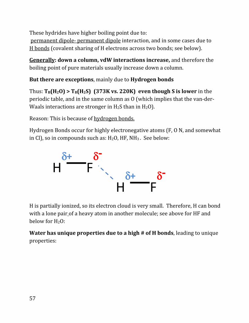
Hydrogen Bonds occur for highly electronegative atoms (F, O N, and somewhat
in Cl), so in compounds such as: H2O, HF, NH3 . See below:
H is partially ionized, so its electron cloud is very small. Therefore, H can bond
with a lone pair of a heavy atom in another molecule; see above for HF and
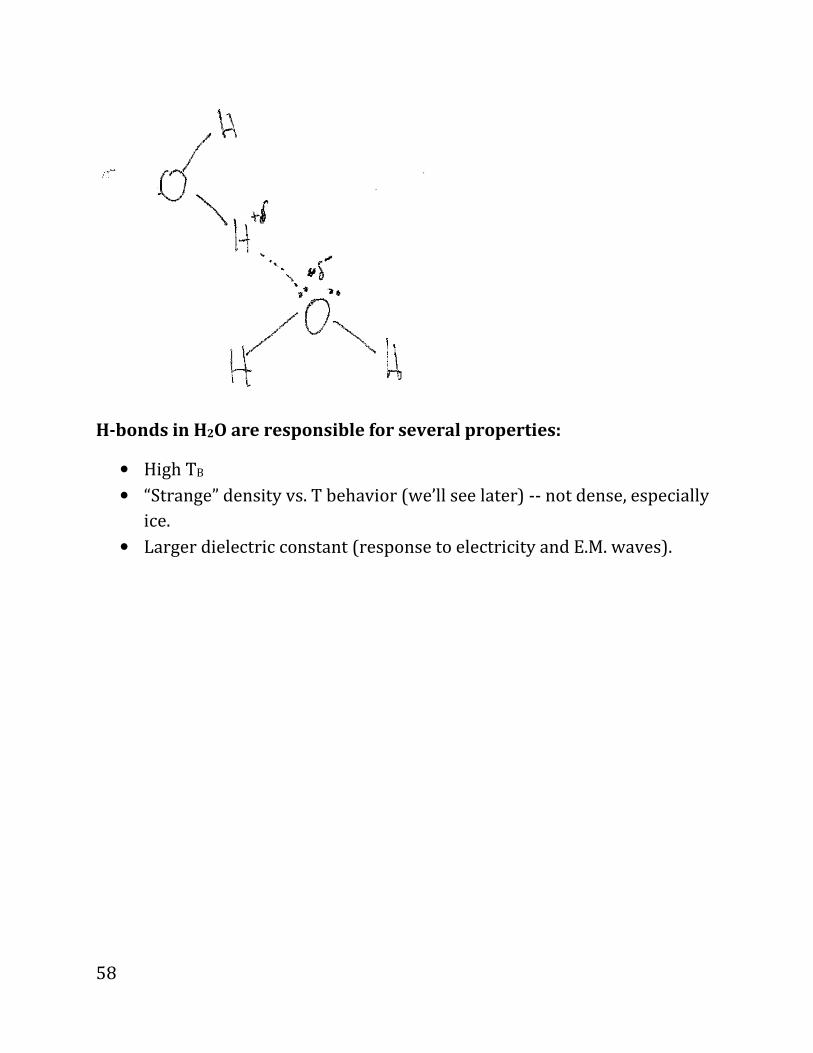
below for H2O:
Water has unique properties due to a high # of H bonds, leading to unique
properties:
Hδδδδ+
Fδδδδ-
H
δδδδ+
Fδδδδ-
58
H-bonds in H2O are responsible for several properties:
• High TB
• “Strange” density vs. T behavior (we’ll see later) -- not dense, especially
ice.
• Larger dielectric constant (response to electricity and E.M. waves).

59
Part 3: Phases and Phase equilibrium:
Overview:
• Phases
• Phase transitions
• Gas-liquid isotherms
• H2O phase diagram
• The Solid-Liquid boundary
Samples that are homogenous in chemical comp. and physical state are called
phases.
There can be 2 or more phases present at the same time (coexist); e.g., ice-water.

60
Another example: liquid-vapor transition:
Simplest: closed laundry room (with wet cloths) or closed pool “feeling very
humid”.
In experiments:
• Evacuate flask
• Introduce liquid that does not fill up volume
• Monitor P
Peq : “ vapor pressure”: (E.g., PH2O(Troom) = 0.035 bar; I.e., in an enclosed pool,
with 100% humidity, 3.5% of molecules are water.)
Also note:
Initially
empty
Then:
Inject liquid
with syringe
Later on: some fluid
spontaneously evaporates,
Non-zero pressure.
Syringe
T P
vapor

61
Microscopic picture:
At any time some molecules get through collisions enough E to leave liquid
Also: gas molecule collide back & trapped in liquid.
So: Equilibrium results when P=Peq(T)
Phase eq.: dynamic, molecules leave and join;
In average the number of molecule in liq. and gas is fixed in equilibrium.
Since: the rates of gas-to-liquid conversion and liquid-to-gas conversion will be
equal in equilibrium, the number of molecules in each phase is unchanged.
Note:
Our description was for the case that initially the flask contained only liquid (no
vapor initially), so we schematically write:
H2O(Liq.)�H2O( Liq.).
If initially there’s no liq., and we instead pump vapor in, then the gas will liquefy:
H2O(Gas)� H2O( Liq.).
62
Finally: what happens if another gas, e.g., air is present?
Answer: nothing really changes as far as the water vapor and pressures!
The air pressure simply adds up with the water pressure to give the total
pressure
Ptotal= Peq H2O(T) + Pair
So for example at room temperature, if we have 100% humidity (e.g., water in a
balloon), then Peq, H2O(T=298K)~ 0.035 P0, so if the total pressure is P0 (sea
level), then Pair~ 0.965P0.
63
Tfreezing
T
gas
water
ice
P=fixed
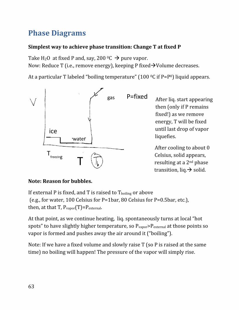
Phase Diagrams
Simplest way to achieve phase transition: Change T at fixed P
Take H2O at fixed P and, say, 200 0C � pure vapor.
Now: Reduce T (i.e., remove energy), keeping P fixed�Volume decreases.
At a particular T labeled “boiling temperature” (100 0C if P=P0) liquid appears.
After liq. start appearing
then (only if P remains
fixed!) as we remove
energy, T will be fixed
until last drop of vapor
liquefies.
After cooling to about 0
Celsius, solid appears,
resulting at a 2nd phase
transition, liq.� solid.
Note: Reason for bubbles.
If external P is fixed, and T is raised to Tboiling or above
(e.g., for water, 100 Celsius for P=1bar, 80 Celsius for P=0.5bar, etc.),
then, at that T, Pvapor(T)=Pexternal.
At that point, as we continue heating, liq. spontaneously turns at local “hot
spots” to have slightly higher temperature, so Pvapor>Pexternal at those points so
vapor is formed and pushes away the air around it (“boiling”).
Note: If we have a fixed volume and slowly raise T (so P is raised at the same
time) no boiling will happen! The pressure of the vapor will simply rise.
64
Another way to achieve phase-transition: change P at a fixed T.
Fix T, and P
At P=Peq(T) condensation; above Peq(T), vapor turns to liquid.
(At very high pressure: liquid solidifies.)
Another way to look at phase transitions:
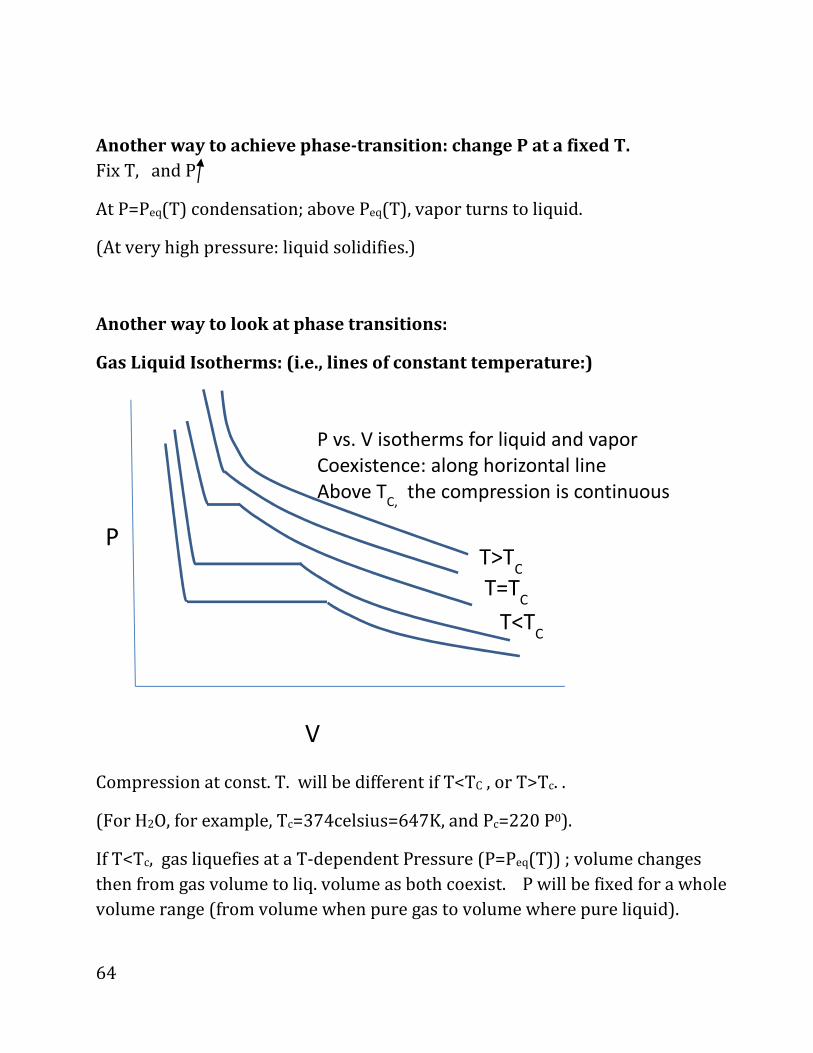
Gas Liquid Isotherms: (i.e., lines of constant temperature:)
Compression at const. T. will be different if T<TC , or T>Tc. .
(For H2O, for example, Tc=374celsius=647K, and Pc=220 P0).
If T<Tc, gas liquefies at a T-dependent Pressure (P=Peq(T)) ; volume changes
then from gas volume to liq. volume as both coexist. P will be fixed for a whole
volume range (from volume when pure gas to volume where pure liquid).
T<TC
V
T=TC
T>TC
P
P vs. V isotherms for liquid and vapor
Coexistence: along horizontal line
Above TC,
the compression is continuous

65
This is what happens to water at room pressure P0 at 100 Celsius; then, as we
lower the volume it will change, for one mole, from about 31L (idea gas molar
volume for temperature of 100 Celsius), to about 0.02Liter for pure liquid, all
the while P being kept at one bar.
But for T>Tc : g� liq. continuously without a phase change when T (and
therefore thermal energy) is high enough to overcome binding.
Note: we use g (gas) and v (vapor) interchangeably!!!
66
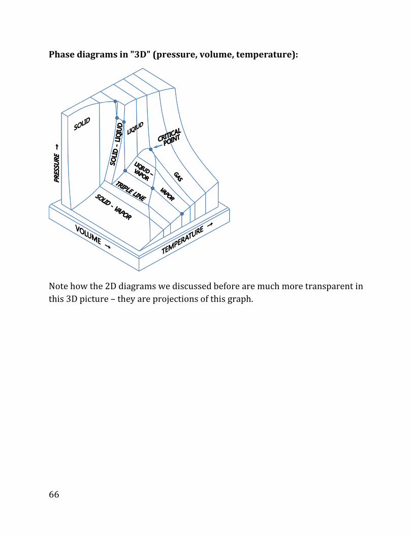
Phase diagrams in "3D" (pressure, volume, temperature):
Note how the 2D diagrams we discussed before are much more transparent in
this 3D picture – they are projections of this graph.

67
Phase Diagrams for H2O: (taken from gi.alska.edu)
In this figure:
m.p. = normal meting point: T(s�l) at 1atm (273K)
b.p. = normal boiling point: T(l�v) at 1atm, 373K (100 celsius)
t.p. = triple point; P,T at which l, v, s coexist
(for H2O: 0.001Celsius, 0.006 bar)
Tc, Pc: above which there are no l/v phase transitions, just gradual transition;
called “supercritical region;
In the supercritical region it isn’t possible to uniquely say “liq.” or “vap.” .
(Note that At high pressures,2000 bar and afovee, other (more compressed)
solid phases appear, different from the “usual” ice).

68
Phase diagrams: the S/L boundary
Water and few other substances: V(solid)>V(liq.)
(E.g., water bottle crack in freezer as water�ice).
For these substance, as P increases, substances prefer to be more liquid like
(lower V)� so at the same pressure liquid preferred.
Therefore, for water & few others:
(This effect is very weak however! Need
huge P increases to change Tmelting by
1K!)
For most substances, the opposite
behavior, since usually:
V(solid) <V(liquid),
so
P ↑ Tmelting ↓ (most substances)
(again, a weak effect).
The special behavior of water is called:
“Anomalous” dependence of the S/L boundary on pressure.
It is due to hydrogen bonds, due to which ice has a big volume:
P , Tmelting
(H2O) H2O,
few other
substances
Most
substances

69
Part 4: Solutions
Topics:
• Mole fractions, molarity, molality
• Molality.
• Macroscopic nature of dissolved species.
• Solution reaction stoichiometry
Solution is : A “homogenous system with 2 or more substances” (usually liquids
or gases)
Composition measures:
Mole fraction of a substance “i”
ÐÑ . AÑAÒÅÒ
Sum of the mole fractions is 1:
ÓÐÑ .Ó AÑAÒÅÒÑÑ. 1AÒÅÒ ÓAÑ . AÒÅÒAÒÅÒÑ
. 1
ÓÐÑ .Ñ1
(e.g., salty water could be 5% salt and 95% water, together 100%).
Other measures beyond mole fraction:
Molarity:
�W^89QRS . �¡¢À£¡Ô£¡¢ÕÂÀÌÖÂÀ×£¡Ô£¡¢ØÀà(mol/L)
Measure: M = (definition): mol/L.

70
Example:
0.2 mole of NaOH in 20 Liter of H2O: molarity = 0.2 mol/20L = 0.01 M
Another measure is: Molality:
�W^8^QRS . �¡¢À£¡Ô£¡¢ÕÂÀ¦ ¡Ô£¡¢ØÀà(mol/Kg)
Molarity will change with T if V changes; Molality won’t change with T, so it is
easier to use.
INSERT (as always, required): Different composition measures can be
related:
E.g., take the example of a binary solution:
ÐÙÐÚ .ÛÜÛÝÞÝÛßÛÝÞÝ
. AÙAÚ
i.e., (since XA + XB = 1)
ÐÙ1 − ÐÙ = AÙAÚ
So, if B is solvent (e.g., water) and A is solute, then, we define
Molality ≡ ÛÜUàÈÈ*Ú&
. AÙAÚ ∗ �W^. �8NN*á&
. �UÅâ.UàÈÈ*Ú& ÛÜÛß = (using the Eq. above:)
Molality . 1�W^. �8NN*á& Ðã1 − XA
END OF INSERT
71
Macroscopic Nature of Dissolved Species
Dissociation of a species (the “solute”) in a solution (i.e., in a “solvent”), is caused
by combination of 3 effects
1. Solute-solute bonds break (loss of attraction, not favorable)
2. New I.M. bonds form between solute and solvent (gain of attraction,
favorable)
3. There is much more “disorder”, which increases the possibilities for
dissociating (favorable); we’ll study this later.
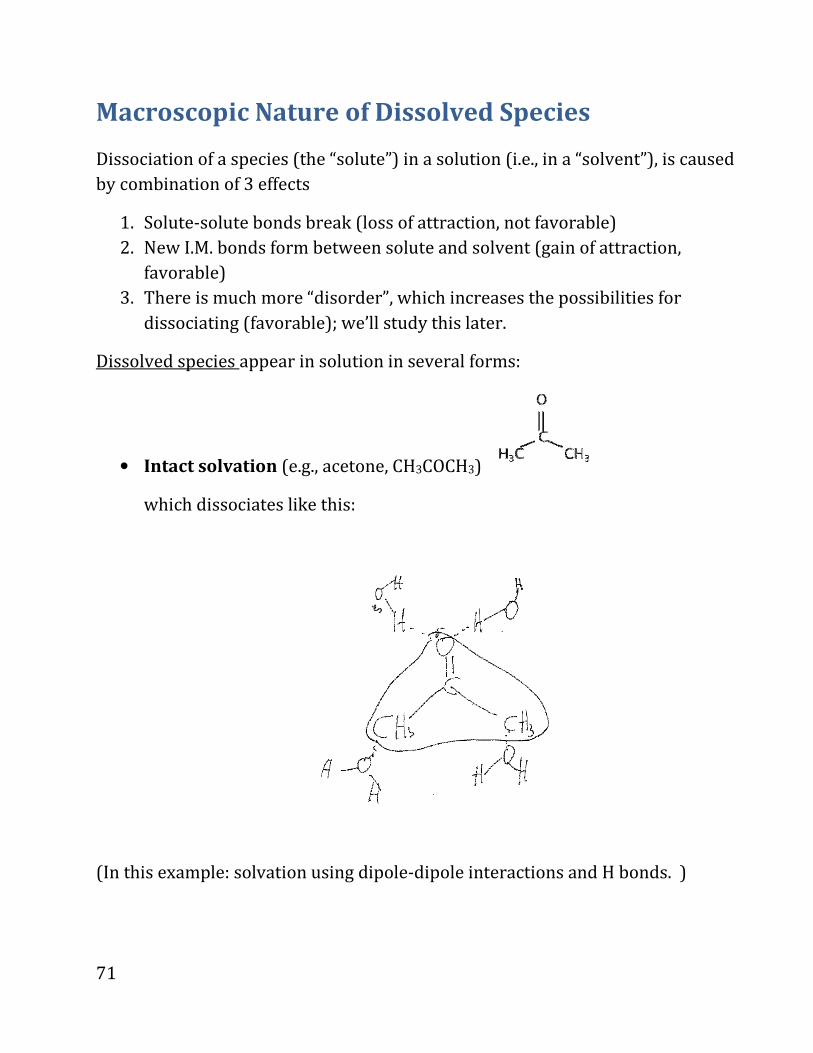
Dissolved species appear in solution in several forms:
• Intact solvation (e.g., acetone, CH3COCH3)
which dissociates like this:
(In this example: solvation using dipole-dipole interactions and H bonds. )
72
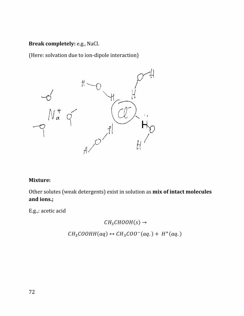
Break completely: e.g., NaCl.
(Here: solvation due to ion-dipole interaction)
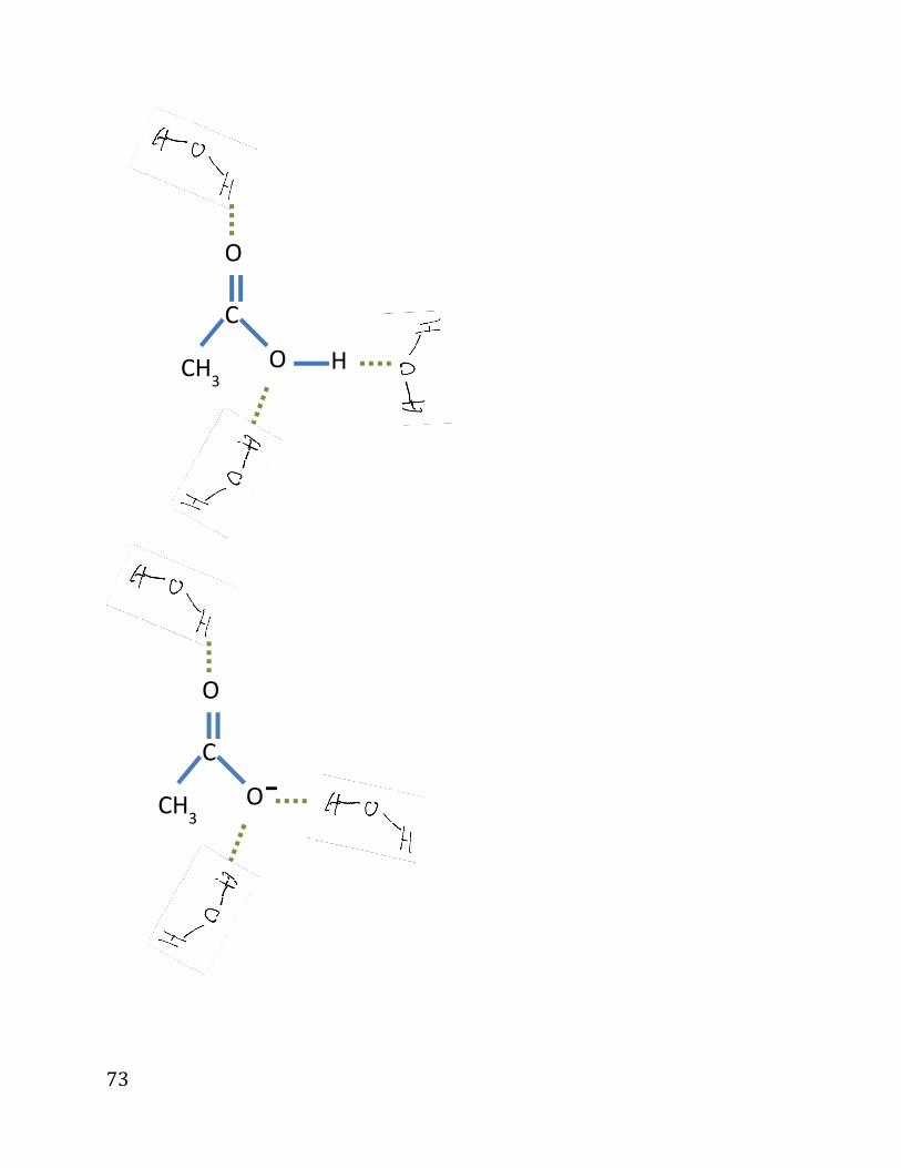
Mixture:
Other solutes (weak detergents) exist in solution as mix of intact molecules
and ions.;
E.g.,: acetic acid
¬¨,¬¨¹¹¨*N& →
¬¨,¬¹¹¨¨*8å& ↔ ¬¨,¬¹¹»*8å. & + ¨ç*8å. &
H
73
C
O
CH3
O H
C
O
CH3
O -

74
INSERT: Solutions rxn. Stoichiometry (not covered in class, but
you will need to know this!)
Vast majority of chem. rxns. happen in solution.
Need to convert stoichiometry of rxns. to eqns. for concentrations rxns.
Schematically, 3 steps are needed:
• Concentrations of reactants � Volumes and Molar quantities
• Volumes and Molar quantities � # moles of products
• # moles of products � concentrations of reactants
Example:
2Br»*aq. & + Cl�*aq. & → 2Cl»*aq. & + Br�*aq. &
Question: Say we have 75mL of 0.08M solution of NaBr. (M means: mol/L)
1) What’s the Volume of 0.03M Cl2 solution that’s needed to react completely
with Br» ?
2) What’s the conc. of Cl» in resulting solution.
Answer:
First: note that NaBr essentially breaks completely to Na+, Br-
We know the Volume � get # of moles of reactants
# moles Br» = Vol.(L) * conc.(M) = 0.075L * 0.08 M
=6 ∗ 10»,�W^ [Remember: M = mol/L].
To learn from this about the products, we’ll use:
RXN. Stoichiometry:
1mol. Cl2 reacts with 2 mol of Br- � 3 ∗ 10»,�W^ of Cl2 reacts with 6 ∗ 10»,�W^ of Br-
So: The answer to (1), i.e., the volume of the Cl2 necessary to react with Br--:

75
?*Cl�NW^XRQWA& . #�W^YWAY. eUÅâg i = 3 ∗ 10»,�W^3 ∗ 10»��W^/é . 0.1é = êëëìí
Note that when mixing 75mL of 0.08 M NaBr with 100mL of 0.03 M Cl2 , final
volume is about 175mL (not exactly, since molecules in solution rearrange to
have smaller or higher volume, but we’ll approximate that the rearrangement
effect is small and does not change the total volume appreciably).
So assuming rxn. goes completely to products (recalling that for every Cl2 mole
we produce 2 moles of Cl» , so 3*10-3 mol of Cl2 will give 6*10-3 moles of the ion):
¬WAY. WC¬^» . #�W^WC¬^ d?W^ . 6 ∗ 10»,�W^0.175é . 3.4 ∗ 10»� �W^é = 0.034T
i.e.,
îïð»ñ . ë. ëwòv
END OF INSERT

76
Parts 5-7: Thermodynamics
Overall Aim in chemistry:
• What reacts?
• How far reactions goes?
• T, P effects on rxn.
• Energy liberated or absorbed.
• How to optimize rxn.
Along the way, study lots of physics (engines, efficiency, energies, etc.)
Part 5: The first law.
Overview:
• Reversible, irrev. processes, energy
• Work and Heat
• First law
• q, w and U in specific cases
• Enthalpy
• Heat capacity
77
Reversible, irrev. processes, energy
Definitions:
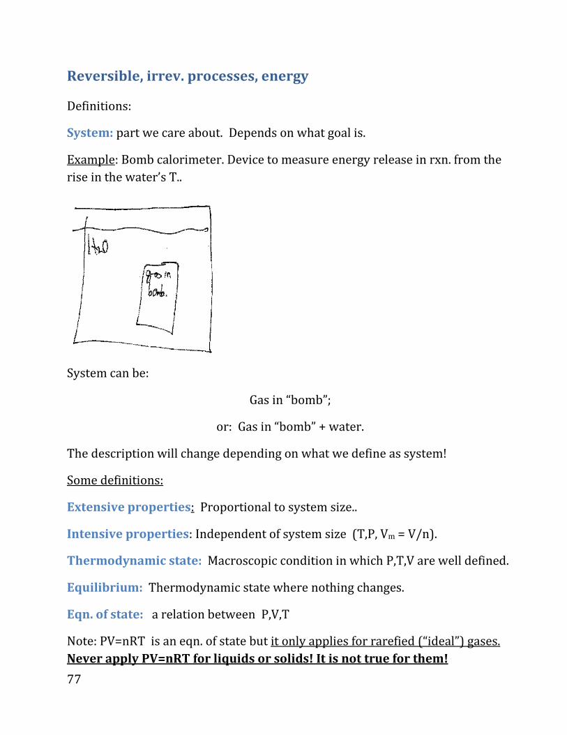
System: part we care about. Depends on what goal is.
Example: Bomb calorimeter. Device to measure energy release in rxn. from the
rise in the water’s T..
System can be:
Gas in “bomb”;
or: Gas in “bomb” + water.
The description will change depending on what we define as system!
Some definitions:
Extensive properties: Proportional to system size..
Intensive properties: Independent of system size (T,P, Vm = V/n).
Thermodynamic state: Macroscopic condition in which P,T,V are well defined.
Equilibrium: Thermodynamic state where nothing changes.
Eqn. of state: a relation between P,V,T
Note: PV=nRT is an eqn. of state but it only applies for rarefied (“ideal”) gases.
Never apply PV=nRT for liquids or solids! It is not true for them!
78
For example: for liquids, e.g., water, when P rises and T is fixed, V barely
decreases! While for gases, when P rises and T is fixed, V shrinks!
Reversible processes: a type of transition between states which proceeds
through continuous series of thermodynamic states, and can be reversed at any
stage
Irreversible: Otherwise.
EXAMPLE: Start piston at P1, V1, T1, and n; End at P2,V2,T2, and same n. (P2>P1,
V2<V1)
If the transition between 1 and 2 is through gradual slow increase of pressure
and compression of the volume, then the transition is reversible;
But if the transition happens by placing a large mass on top of the piston and
suddenly letting it go, then the process will be irreversible (the piston will
compress and expand back and forth until eventually it will settle down at the
new volume); i.e., throughout, P may not even be defined, only at the end.
79
Work and Heat, 1st Law, path dependent (q, w) vs. path
independent quantities. Work as area.
There are two different types of energy transfer.
Heat: E transfer by thermal contact
Work: Ordered transfer (mechanical pushing or electron current).
Heat example:
Throw an iron bar with a hot T (Tiron) to water at a colder temp., Twater; there will
be a transfer of thermal energy from the hotter object (the bar) to the colder one
(water) and the eventual systems will be iron+water at a temperature Tf which
is in between Tiron and Twater.
This energy transfer is called “heat”, denoted by q, and has energy units.
80
Work derivation and example
First and foremost we’ll consider mechanical work (“pushing”) (electrical work
will be considered much later, in the context of batteries).
Work= energy transfer. (units: J)
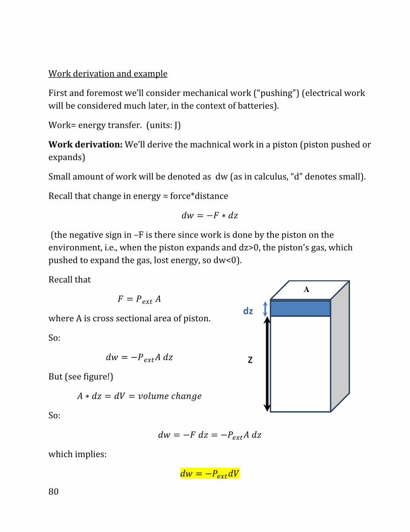
Work derivation: We’ll derive the machnical work in a piston (piston pushed or
expands)
Small amount of work will be denoted as dw (as in calculus, “d” denotes small).
Recall that change in energy = force*distance
O_ . dV ∗ Oó
(the negative sign in –F is there since work is done by the piston on the
environment, i.e., when the piston expands and dz>0, the piston’s gas, which
pushed to expand the gas, lost energy, so dw<0).
Recall that
V . 4Ç�Òã
where A is cross sectional area of piston.
So:
O_ . d4Ç�ÒãOó
But (see figure!)
ã ∗ Oó . O? . �W^X�PYZ8A[P
So:
O_ . dVOó . d4Ç�ÒãOó
which implies:
O_ . d4Ç�ÒO?
81
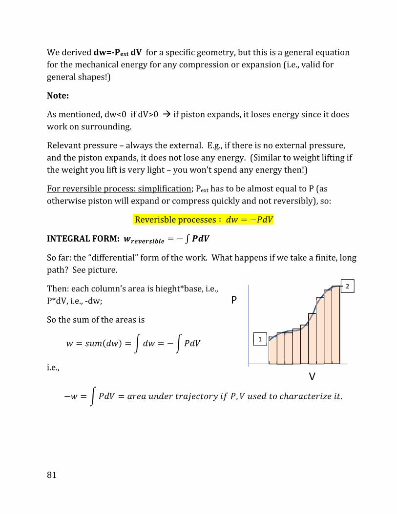
We derived dw=-Pext dV for a specific geometry, but this is a general equation
for the mechanical energy for any compression or expansion (i.e., valid for
general shapes!)
Note:
As mentioned, dw<0 if dV>0 � if piston expands, it loses energy since it does
work on surrounding.
Relevant pressure – always the external. E.g., if there is no external pressure,
and the piston expands, it does not lose any energy. (Similar to weight lifting if
the weight you lift is very light – you won’t spend any energy then!)
For reversible process: simplification; Pext has to be almost equal to P (as
otherwise piston will expand or compress quickly and not reversibly), so:
Reverisbleprocesses ∶ O_ . d4O?
INTEGRAL FORM: õö÷ø÷öùúûð÷ . d�üýþ
So far: the “differential” form of the work. What happens if we take a finite, long
path? See picture.
Then: each column’s area is hieght*base, i.e.,
P*dV, i.e., -dw;
So the sum of the areas is
_ . NX�*O_& . �O_ . d�4O?
i.e.,
d_ . �4O? . 89P8XAOP9R98«PYRW9SQC4, ?XNPORWYZ898YRP9QóPQR.
V
P
1
2
82
DIGRESSION ON CALCULUS (not covered in class, but required).
We need to calculate summation over small changes; for example, the amount of
work spent in a process is
dω ω=∑
Where the sum is over all the steps, i.e., we expand (or compress) from the
initial to the final volume, the expansion is done in little steps, in each step the
work is –PdV (where P is the pressure at each step), and add that up.
If you learned calculus, you know that this operation of summing over the
contribution of many small steps is called an integral, and is denoted by a
stretched-S (i.e., a stretched Sum):
final volume 2
initial volume 1
d dω ω ω= =∫ ∫
where we denote by “2” and “1” the final and initial states.
The two integrals you need to know are:
2
2 11
dx x x= −∫
(This is obvious – the sum of volume changes is the difference between the final
and initial volume), and
22
11
lndx x
x x
=
∫ .
(If you never saw this, accept it till you study calculus). Note that we use here
ln, i.e., logarithm in base “e”, where e=2.7….
Finally, if there’s a constant we can take it out of the integral, e.g.,
2 2
1 1R dx R dx=∫ ∫
END OF DIGRESSION, BACK TO THERMODYANMICS.

83
The derivation so far leads to the first law, which is nothing more than a
statement that energy is conserved, i.e., any energy transfer can be decomposed
into a heat part and a work part:
First law:
∆½ . å + _
Where:
• ∆½: energy change of system
• q: heat involved in process
• w: work involved in process
To conclude: change in energy is due to heat plus work.
However, we have to carefully understand what each term corrspondes to, see
next page.
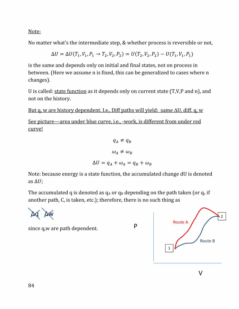
84
Note:
No matter what’s the intermediate step, & whether process is reversible or not,
Δ½ . ∆½*D�, ?�, 4� → D�, ?�, 4�& . ½*D�, ?�, 4�& d ½*D�, ?�, 4�&
is the same and depends only on initial and final states, not on process in
between. (Here we assume n is fixed, this can be generalized to cases where n
changes).
U is called: state function as it depends only on current state (T,V,P and n), and
not on the history.
But q, w are history dependent. I.e., Diff paths will yield: same ∆U, diff. q, w
See picture—area under blue curve, i.e., -work, is different from under red
curve!
åÙ ≠ åÚ
�Ù ≠ �Ú
Δ½ . åÙ + �Ù . åÚ + �Ú
Note: because energy is a state function, the accumulated change dU is denoted
as Δ½;
The accumulated q is denoted as qA or qB depending on the path taken (or qc if
another path, C, is taken, etc.); therefore, there is no such thing as
since q,w are path dependent.
Δq Δw
V
P
1
2
Route A
Route B

85
q and w in specific cases; enthalpy.
Usually it is a pain to measure w; we usually want to find out how much q is, and
furthermore, we want to express q somehow as relating to state functions.
We learned now that this is not possible in the general case, as q is path
dependent.
However, there are specific cases when we can do it.
Assume in the following that there is only mechanical work, i.e., no electrical
current so no electrical work.
Then, the simplest case is :
Fixed Volume:
Then,
�� .d4O? . 0*ifVisfixed, sodV . 0&
So:
O½ . Oå + O� . Oå d 4O? . Oå*forVfixed&
i.e., denoting q by a subscript V to emphasize that we talk about processes where
the volume is fixed throughout,
O½ . Oåg *ifVfixedthroughprocess&
So we can relate the energy and the heat for a fixed volume processes, i.e.,
reaction in a closed rigid flask.
Two notes:
Only valid if V fixed throughout processes;
it is not enough that V( initial) and V(final) are the same.
However: Most reactions take place at fixed P, not fixed V; so need a new
quantity:

86
Enthalpy:
For convenience (we’ll see shortly why) we define a new function, which we
label enthalpy:
¨ . ½ + 4?
This is a general definition. It is especially useful and important however, for one
type of processes, where P is fixed throughout the whole process.
Formally,
O¨ . O½ + O*4?&
If the pressure if fixed, and P=Pext for simplicity (i.e., as in reversible processes),
then
O¨ . O½ + 4O?
(This is because P is constant through the process! )
On the other hand, the 1st law gives:
O½ . Oå + O� . Oå d 4O?
So therefore:
VW9CQPO]9PNNX9P:O¨ . O½ + 4O? . Oå d 4O? + 4O? . Oå
i.e., for a process where the pressure is fixed throughout (so q is labeled by
subscript p):
O¨ . Oå�*forfixedPprocessonly!&
And if we accumulate over many changes, the change in enthalpy will be related
to the heat given/taken:
∆¨ . å�*forfixedPprocessonly!&
Therefore, we don’t have to worry about measuring pressures and volume if we
do a process at fixed pressure; we can measure the enthalpy change directly
87
from the amount of heat input into/from the system, which is usually an easy
task.
Conversely, enthalpy is a state function, which means it can be tabulated, so we
can calculate amounts of heat given/taken from the system by using tabulated
enthalpy differences; but this is only true if the pressure is fixed!
Since in real life we do experiments in labs, where usually the pressure is fixed
(at 1atm or similar value), enthalpy is very useful.
Finally, some definitions for later. For a fixed P process:
∆¨ < 0 → å� < 0*heatreleasedbysystematfixedPprocessifenthalpydecreases&
Such ∆¨ < 0 processes are called exothermic (since heat is released – “exo”
means to output in this context).
And conversely there are endothermic processes where heat is absorbed:
∆¨ > 0 → å� > 0
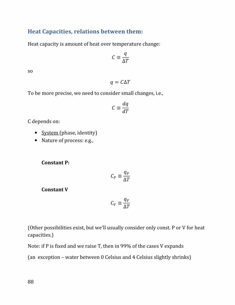
88
Heat Capacities, relations between them:
Heat capacity is amount of heat over temperature change:
¬ ≡ å∆D
so
å . ¬∆D
To be more precise, we need to consider small changes, i.e.,
¬ ≡ OåOD
C depends on:
• System (phase, identity)
• Nature of process: e.g.,
Constant P:
¬� ≡ å�∆D
Constant V
¬g ≡ åg∆D
(Other possibilities exist, but we’ll usually consider only const. P or V for heat
capacities.)
Note: if P is fixed and we raise T, then in 99% of the cases V expands
(an exception – water between 0 Celsius and 4 Celsius slightly shrinks)
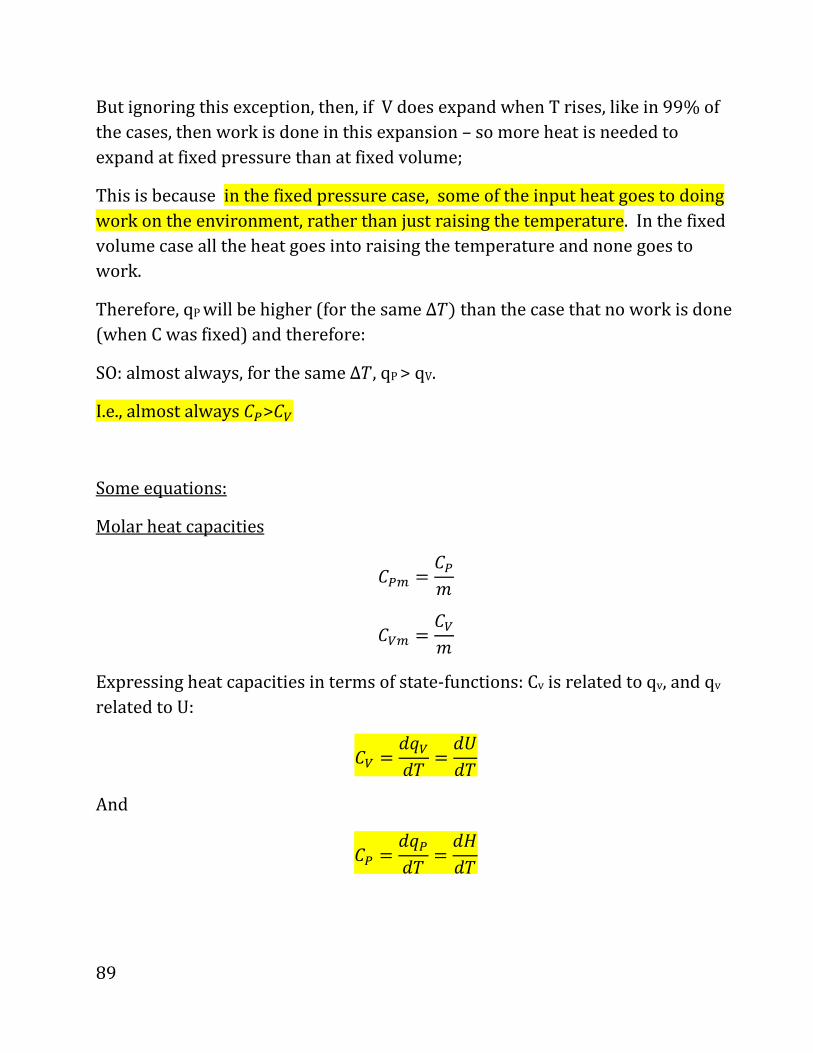
89
But ignoring this exception, then, if V does expand when T rises, like in 99% of
the cases, then work is done in this expansion – so more heat is needed to
expand at fixed pressure than at fixed volume;
This is because in the fixed pressure case, some of the input heat goes to doing
work on the environment, rather than just raising the temperature. In the fixed
volume case all the heat goes into raising the temperature and none goes to
work.
Therefore, qP will be higher (for the same∆D& than the case that no work is done
(when C was fixed) and therefore:
SO: almost always, for the same ∆D, qP > qV.
I.e., almost always ¬�>¬g
Some equations:
Molar heat capacities
¬�U . ¬��
¬gU . ¬g�
Expressing heat capacities in terms of state-functions: Cv is related to qv, and qv
related to U:
¬g . OågOD . O½OD
And
¬� . Oå�OD . O¨OD
90
Actual relations between heat capacities
• For solids and liquids very little work will happen when the temperature
rises (since the total volume is very small, and therefore the volume
change is even smaller) so:
There will be very little difference between qP and qV for
solids/liquids.
And therefore:
ïü is almost equal to (very slightly larger usually from) ïþ for
solids/liquids.
• Gases:
Note that for ideal gases:
¨ . ½ + 4? . ½ + AED*QOP8^[8NPNWA^S&
So (we fudge the math. a little, but that’s OK):
¬� d ¬g . O¨OD d O½OD . O*¨ d ½&OD . OAEDOD . AE
i.e., for ideal gases only
¬� . ¬g + AE*idealgasesonly‼!!&

91
Qualitative considerations on the heat capacities for ideal gases,
and examples:
An interesting fact (no proof here:) Each degree of freedom that’s “active”
contributes R/2 to ïþì
Note on “active” degree-of-freedom: we learned when we talked about the
Boltzmann factor that if there is a degree of freedom such that its excitation
energy is very high compared with RT, then it will be in the ground state, i.e., will
not be excited, and will therefore not contribute to heat-capactity
Examples:
Monatomic ideal gas: can move in x, y, z directions� 3 degrees of freedom �
Cvm (He, etc.)= 3R/2
Diatomic ideal gas like O2 around T(room): in addition to center-of-mass moving
in the x, y, z direction, the diatomic “rod” can rotate in 2 directions (but cannot
vibrate unless T is very high) � 5 degrees of freedom
Cvm (O2,etc.)= 5R/2 10K<T<1000K
Note:
• below ~10K rotations not excited;
• above 1000K vibrations need to be included as thy get excited; specifically,
at room temperature O2 does not vibrate, and it needs very high
temperatures (higher than 1000K) to vibrate. But at high temperatures
(more than say 1500K) it will vibrate freely, so its CVm will be higher than
5R/2.
Therefore:
For monatomic gas (He, etc.):
3 5
, 2 2
Vm Pm
R RC C= =

92
For O2 and similar:
5 7,
2 2Vm Pm
R RC C= =
Note that the heat capacity changes (increases) as we go to bigger molecule
(more degrees of freedom), but the relation CP=CV+nR is valid for any (ideal) gas
(proof : 110A)
Detailed discussion of this figure.
Note that the heat capacity of oxygen is 3R/2 at very low temperatures, where the
only motions are of the center of mass (rotations cannot be done since they require
energy and there is not enough energy at low temperatures)
At a large range between very low temperatures and very high temperatures,
10K<T<1000K the fixed-volume heat capacity (CVm) is 5R/2, since to the 3R/2
from the center of mass motion we add 2 more degrees of freedom associated
with rotations perpendicular to the diatomic axis,
I.e., if the diatom is in the z direction, there will be rotations around the x and
around the y directions; rotations around the z axis do not contribute since they
don’t involve motion of nuclei.
CPm
CVm
93
Each degree of freedom gives R/2 to CVm, so altogether we have:
¬gf . 3E2 + 2 ∗ E2 . 5E2 At very high temperatures when the vibrational degrees of freedom contribute,
CVm becomes even higher (7R/2, and then even higher).
At every temperature, CPm=CVm+R for ideal gases, as we will not prove (but will
use).
Solids and liquids heat capacity-repeat
As mentioned, for solids and liquids the Cp=Cv + nR relation is not true; instead:
P V
C C≅ for solids, liquids.
The reason is that the volume of solids and liquids is very small, and not
changeable easily, so very little work can be done on solids and liquids.
The properties of solids and liquids – including volume and entropy, as we'll see
below -- are mostly determined by the temperature. Thus, we get that in some
respects they are analogous to ideal-gases, their extreme opposite, since in ideal
gases the energy depend solely on temperature.
However, the analogy cannot be pushed too far, since in ideal gases the volume
depends on pressure, and for solids and liquids (within the same phase) it
usually hardly changes with pressure.
94
Reversible processes in i.g. (ideal gases): isothermal expansion
and adiabatic expansion
Useful to demonstrate laws and importance in thermodynamics.
Say we do a reversible isothermal expansion of ideal gases: State 1� state 2.
(Isothermal expansion (or compression) means that T is fixed, while P and V
vary.)
Τhen, ∆U=0 (since T is fixed and we know that for ideal gases, U is only a
function of T).
Also:
2
1
2
1
d
PdV
ω ω
ω
=
= −
∫
∫
where P is dependent on the volume as P=nRT/V (true only for ideal gases!)
2
1
nRTdV
Vω
= −
∫
Since nRT is fixed in isothermal expansions , take it of the integral:
(We used � �� . ln eg©g�i ).
What about q? well, recall thT
2
1
2
1
ln
dVnRT
V
VnRT
V
ω
ω
= −
= −
∫

95
2
1
And for isothermal expansion, U=0, so
0
ln
q U
q
Vq nRT
V
ω
ω ω
= ∆ −
∆
= − = −
=
Example: see figure.
In this figure example: w=-nRT ^A eÊ5��Ê�i
= -(1mol*8.3J/(K mol)*300K) * ln(2)
= -2500 J *0.693 = -1730J
q = ∆U -w = 0-(-1730J) = 1730J
96
Ostensible problem with isothermal expansion:
How come we input heat, and the temperature does not rise?
Answer:
Imagine a runner that continuously eats and drinks while she runs – she
continuously converts the food and drink to energy used in running, so her body
weight does not change.
Same here: the work that is done by the gas is compensated by the heat given to
the gas, so the energy does not change (and therefore the temperature can stay
fixed).
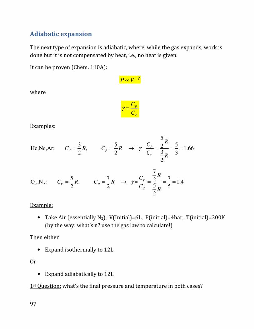
97
Adiabatic expansion
The next type of expansion is adiabatic, where, while the gas expands, work is
done but it is not compensated by heat, i.e., no heat is given.
It can be proven (Chem. 110A):
P Vγ−∝
where
P
V
C
Cγ =
Examples:
5
3 5 52He,Ne,Ar: , = 1.6632 2 3
2
P
V P
V
RC
C R C RC
R
γ= = → = = =
2 2
7
5 7 72O ,N : , = 1.452 2 5
2
P
V P
V
RC
C R C RC
R
γ= = → = = =
Example:
• Take Air (essentially N2), V(Initial)=6L, P(initial)=4bar, T(initial)=300K
(by the way: what’s n? use the gas law to calculate!)
Then either
• Expand isothermally to 12L
Or
• Expand adiabatically to 12L
1st Question: what’s the final pressure and temperature in both cases?

98
Answer:
• Isothermal expansion:
T=fixed � T(final)=T(initial)=300K
P(final): since P=nRT/V, and T did not change while V doubled �
Therefore, P was halved, i.e., P(final)=4bar/2= 2bar
• Adiabatic expansion:
Fast way of getting the result: V doubled (increases by a factor of 2); so P,
which is proportional to V γ− , changes by a factor of 2 γ− , i.e.,
P(final) = P(initial)* 2 γ− = 4bar * 1.42− = 1.52 bar.
What about T? Since
D . 4?AE ,
and since V doubled and P decreases from 4bar to 1.52 bar, then
( ) ( ) ( ) 1.52 12 1.52 12
0.76( ) ( ) ( ) 4 6 4 6
T final P final V final bar L
T initial P initial V initial bar L= = • = • =
i.e., T(final)=T(initial)*0.76=300K*0.76=228K.
2nd question: How much work was done in the adiabatic expansion?
Answer:
The answer deserves a separate section:
99
Calculating work in adiabatic expansion.
We could have used
w PdV= −∫
But that will be a difficult integral. Instead, use:
q Uw U∆ − = ∆=
where we noticed that in adiabatic expansion q=0. So all we need is the change
in U, the internal energy.
Here comes a non-trivial point: for ideal gases (and only for ideal gases), as
we consider, the energy depends only on temperature. Therefore, if we
change the temperature in the adiabatic process, we can calculate the
energy change by considering ANY OTHER process where the temperature
changed by the same amount (even if the final volume and pressure are
different).
The simplest such 2nd process is a fixed volume process with the same
temperature change; In other words, since
dU=CVdT
for fixed volume process, then we know that dU=CVdT here, even though V is not
fixed!
(Note that I am only talking about dU; dq and dw will be different in each of
these processes -- - in one, dq=0 (adiabatic); in the other, dV=0 so dw=0 and
dq=dU; but the energy change is the same in both processes, even though the
final states are different – because the final temperature are the same in both!)
For the fixed volume case:
V V VmU T TC dT C C n∆ = ∆= = ∆∫

100
And therefore in our case (where the volume isn’t fixed, but T changes by the
same amount!) we get the same energy change, i.e.,
(ideal gas,Vnot necess. fixed) VmC nU T∆ = ∆
and we know each of the terms:
228 300 72
/ ( ) (when calculated for the initial conditions, as n does not vary)
4 6 24
8.3 300 mol
5 / 2 =2.5*(8.3 J/(K mol)) =20.7 J/(K mol) (for air at reasonable T's)Vm
f iT T K K K
n PV RT
bar Ln
J
T
K
C R
K
=
− =∆ = − = −
= =
•= =
00J0.96
2500( / )mol
J mol=
We can calculate now
J20.7 *0.96 mol*(-72K)=-1430J
K molVmC nU T∆ = ∆ =
So in this adiabatic expansion, 1.43kJ of work was done by the system.
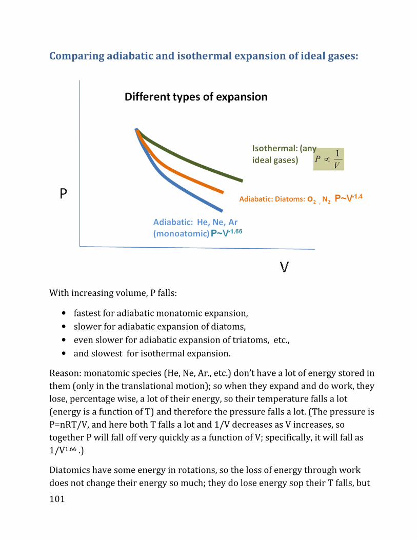
101
Comparing adiabatic and isothermal expansion of ideal gases:
With increasing volume, P falls:
• fastest for adiabatic monatomic expansion,
• slower for adiabatic expansion of diatoms,
• even slower for adiabatic expansion of triatoms, etc.,
• and slowest for isothermal expansion.
Reason: monatomic species (He, Ne, Ar., etc.) don’t have a lot of energy stored in
them (only in the translational motion); so when they expand and do work, they
lose, percentage wise, a lot of their energy, so their temperature falls a lot
(energy is a function of T) and therefore the pressure falls a lot. (The pressure is
P=nRT/V, and here both T falls a lot and 1/V decreases as V increases, so
together P will fall off very quickly as a function of V; specifically, it will fall as
1/V1.66 .)
Diatomics have some energy in rotations, so the loss of energy through work
does not change their energy so much; they do lose energy sop their T falls, but
102
not as much as monatomic species. So their P will not fall as much as for
monoatoms.
Similar reasoning explains that the bigger the molecules of an ideal gas, the
more they have energy stored in them, and therefore the less they will be
affected by the work done through the expansion, and therefore, their T will not
be so affected so their P will not fall so much.
At the extreme is isothermal expansion, now of all species (whether He, O2, or of
any other ideal gas). Here, T does not fall (the energy done by work is
replenished) so their P falls only because P=nRT/V and V increases.
103
Tabulated Enthalpy
We need to define an enthalpy or energy scale, where one of them is zero.
Physicists have a general definition but it is very complicated to use in practice,
so we revert to the practical definition of chemists.
In practice, of course, it rarely matters since we are generally interested in
enthalpy differences (i.e., in the amount of heat spent in a reaction at constant
pressure)
So, as a prelude to the practical definition of enthalpy, we need “standard states”
of each species:
We define
A standard state: 1atm, specific T=298K=25 OC.:
For gases: we assume an ideal gas behavior.
For dissolved specifies: the definition used is an annoying one. We assume that
the species is at a 1M (1 mol/Liter) solution, but not in its real state; instead,
extrapolate from a very low concentration to what the behavior would be at 1M.
Next, we decide that the enthalpy of each element at the standard state, in its
most stable form at the standard state, is assigned to be zero.
We label an enthalpy defined according to this scale as “enthalpy of formation”,
Hf.
For example,
0
2
0
(O , ,298 ,P )=0
( , ,298 ,P )=0
f
f
H gas K
H C graphite K
Note that:
0( , ,298 ,P )>0f
H C diamond K
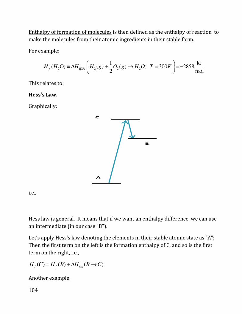
104
Enthalpy of formation of molecules is then defined as the enthalpy of reaction to
make the molecules from their atomic ingredients in their stable form.
For example:
2 2 2 2
1 kJ( O) ( ) ( ) ; 300 2858
2 molf RXN
H H H H g O g H O T K
≡ ∆ + → = = −
This relates to:
Hess’s Law.
Graphically:
i.e.,
Hess law is general. It means that if we want an enthalpy difference, we can use
an intermediate (in our case “B”).
Let’s apply Hess’s law denoting the elements in their stable atomic state as “A”;
Then the first term on the left is the formation enthalpy of C, and so is the first
term on the right, i.e.,
( ) ( ) ( )f f rxnH C H B H B C= + ∆ →
Another example:

105
( ) ( ) ( )f fH A B C H A B D H D C→ + = → + + ∆ →
And in general:
( ) ( ) ( ),
( ) ( ) ( ) ( ),
.
f f
f f f
H B C H B H C
H B C D H B H C H D
etc
∆ → = − +
∆ → + = − + +
Realistic examples: given a table of energy of formations, then how do we
calculate, for room temperature:
2 2
1(2 ) ?
2H NO NO N∆ → + =
Answer
2 2 2 2
2
2 2 2
1 1(2 ) 2 ( ) ( ) ( )
2 2
i.e. (since ( ) 0 )
1(2 ) 2 ( ) ( )
2
2(90.4 kJ/mol) (33.1 kJ/mol) =-147.7 (kJ/mol)
f f f
f
f f
H NO NO N H NO H NO H N
H N
H NO NO N H NO H NO
∆ → + = − + +
=
∆ → + = − +
= − +

106
Part 6: Spontaneity, entropy and 2nd law
The understanding of the 2nd law requires a lot of concepts with which you
are at best barely familiar. So we will try to exemplify and relate the
concepts; but beware that this is a very difficult part, because it is so
qualitative and because these are new concepts.
The order of this chapter is:
• Direction of time in nature is well defined
• Entropy is a measure of disorder; 2nd law: the universe’s entropy rises.
• Thermodynamics definition of entropy changes �� . OåÄÇ�/D
• Examples:
o ideal gas expansion (isothermal, isobaric);
o temperature change of any substance (including solids and liquids)
at fixed pressure (isobaric) or volume,
o Phase change
• Stat. Mech. Definition of entropy: ÈÒàÒ.UÇ��. = �Úln*#WCNR8RPN&
• Entropy tabulation; qualitative understating of how the entropy changes
in chemical reactions.
Direction of time
1st law allows for processes which conserve energy but “don’t make sense”,
E.g., take a physical processes, like a cup falling and breaking;
The “reverse movie” of this processes, which is broken pieces of the cup coming
together spontaneously and becoming one cup, isn’t feasible physically.
Therefore, it isn’t enough to just consider energy when we talk about processes,
we need a law beyond the 1st law.
This is where the 2nd law comes.
It states, essentially, that systems evolve towards equilibrium. (More precise
def.—later).
107
Let’s first exemplify on several processes which always occur in a given
direction in time (i.e., their reverse never occurs):
• Open a balloon at high P; gas always expands out and P is reduced, never
back.
• Two systems initially at different temperatures, TA and TB, when we bring
them in contact, will always reach a temperature Tf which equals in both
• A little of NaCl (table salt, Sodium chloride) in water will always
dissociate.
So: nature is directional in time.
Entropy: measure of disorder; and 2nd law.
So the 2nd law of thermodynamics is:
The Entropy of the world (i.e., the disorder in the world), never decreases;
more precisely: entropy increases if there are irreversible processes and
stays constant for reversible processes.
This is a “law” i.e., something we stipulate and don’t prove, but we can justify it
using some examples based on statistics. If you take a course in statistical
mechanics, you will be able to prove and expand much on the concepts we
introduce.
Thermodynamic entropy
It turns out (no proof) that we can write the change of entropy of a given system
as
thermodynamics definitiondq
dST
=
where dq is the amount of heat if the process is reversible (we’ll review this and
define more precisely later).
Clarification on entropy:
108
• First, the 2nd law talks about the entropy of the universe (that never
decreases). The entropy of a system can decrease, if the entropy of the
surroundings increases. For example, we can cool water (and thereby
decrease their entropy), but when we do it, the entropy of the
surroundings must increase correspondingly, so that the change of
entropy of everything together (the universe) will not decrease.
So: dS can be >0 or <0 or =0, as long as:
SURROUNDING WORLD 0dS dS dS ≥+ =
• Next, consider qualitatively the 1/T in the relation between entropy and
heat, dS=dq/T.
Think of dq as “applied mess”, and of dS as “resulting disorder”
Then we learn that if the temperature is high, the effect of the mess on the
disorder is small (since it is divided by 1/T, and T is high);
But when T is low, a small dq will affect the entropy strongly, as 1/T is large
You know this from daily life: if your dorm room is clean (equivalent to low
T), then a little mess (dq) will make it look quite messy (increase S
significantly);
But if your dorm room is already messy (high T), then making it a little
messier (dq) won't have much of an effect (since dq/T will be small, as 1/T is
small).
• Finally, the entropy change is strictly not dq/T, but
dS=dqrev/T
This means that to calculate an entropy change we must take a reversible path
connecting the initial and final states.
And another thing it tells us: it won’t matter which path we actually take for
entropy changes!
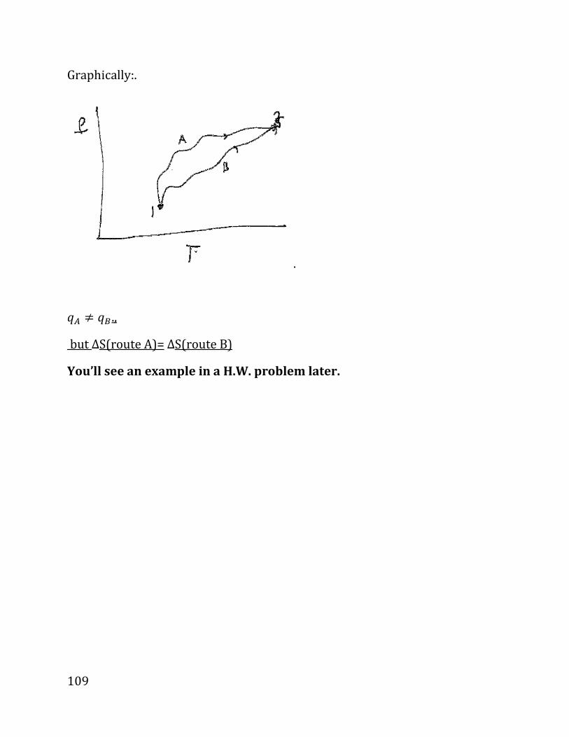
109
Graphically:.
.
åÙ ≠ åÚ .,
but ΔS(route A)=ΔS(route B)
You’ll see an example in a H.W. problem later.

110
Examples for entropy changes, and entropy tabulation.
• Expansion of an ideal gas at constant temperature:
dqdS
T=
Isothermal expansion is a very simple case, since 1/T is fixed during the
expansion. If we start at a volume V0 and end at volume V then (recalling that
q(isothermal expansion)=nRTln(V/V0), as proved):
00
0
1(isothermal) ln
ln
VT
V
qdq nRT VS dq
T T T T V
VnR
V
∆ = = = =
=
∫ ∫
So as V increases, the entropy increases; when the volume doubles, the entropy
increase by nRln[2]. The reason is that as we increase the volume, each particle
has more space to roam through.
For future reference, let’s write isothermal expansion in terms of pressures, and
not volumes (they carry the same info for ideal gas). We know that P=nRT/V, so
4? . 45?5 → gg� . ��� , so
� . AE ln e��� i = −AE ln e���i
Where we’re using
ln eàÆi = ln*8& − ln*7& = −*ln*7& − ln*8&& = − ln eÆài So to conclude:
*D, 4& . *D, 45& + � . *D, 45& d AE ln � 445�
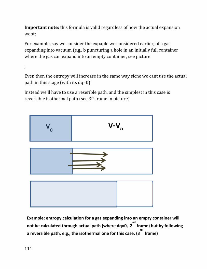
111
Important note: this formula is valid regardless of how the actual expansion
went;
For example, say we consider the expaple we considered earlier, of a gas
expanding into vacuum (e.g., b puncturing a hole in an initially full container
where the gas can expand into an empty container, see picture
,
Even then the entropy will increase in the same way sicne we cant use the actual
path in this stage (with its dq=0)
Instead we’ll have to use a reserible path, and the simplest in this case is
reversible isothermal path (see 3rd frame in picture)
V0 V-V
0
Example: entropy calculation for a gas expanding into an empty container will
not be calculated through actual path (where dq=0, 2nd
frame) but by following
a reversible path, e.g., the isothermal one for this case. (3rd
frame)
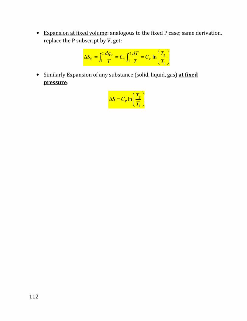
112
• Expansion at fixed volume: analogous to the fixed P case; same derivation,
replace the P subscript by V, get:
2 22
1 11
lnV
V V V
dq TdTS C C
T T T
∆ = = =
∫ ∫
• Similarly Expansion of any substance (solid, liquid, gas) at fixed
pressure:
2
1
lnP
TS C
T
∆ =
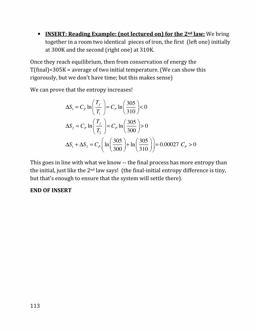
113
• INSERT: Reading Example: (not lectured on) for the 2nd law: We bring
together in a room two identical pieces of iron, the first (left one) initially
at 300K and the second (right one) at 310K.
Once they reach equilibrium, then from conservation of energy the
T(final)=305K = average of two initial temperature. (We can show this
rigorously, but we don’t have time; but this makes sense)
We can prove that the entropy increases!
1
1
2
2
1 2
305ln ln 0
310
305ln ln 0
300
305 305ln ln 0.00027 0
300 310
f
P P
f
P P
P P
TS C C
T
TS C C
T
S S C C
∆ = = <
∆ = = >
∆ + ∆ = + = >
�
This goes in line with what we know -- the final process has more entropy than
the initial, just like the 2nd law says! (the final-initial entropy difference is tiny,
but that’s enough to ensure that the system will settle there).
END OF INSERT

114
• Phase change:
We learned that, since a phase change takes place at a constant P:
(phase change)= Hq ∆
Further, dS=dq/T, and since T is also fixed in a phase change,
phase change
(phase change)(phase change)=
HS
T
∆∆
Example.
Freezing (called “fusion” by chemists/physicists):
Ice->water:
kJ6.0 , T =273K
mol
6000JJmol~ ~ 22
273K K mol
fusion fusion
fusionfusion
fusion
H
HS
T
∆ =
∆→ ∆ =

115
H.W. problem exemplifying that two different paths give the same entropy:
We have a piston of 2 mol, containing He.
The initial point is “1” : T=300K, V=50L, P=1bar. (Verify that PV=nRT!)
The final point is “2”: T=300K, V=100L, P=0.5bar.
Consider then the following two paths (see figure).
Path “A” is isothermal --- i.e., we keep T fixed and just increase the volume from
50L to 100L and the pressure decreases from 1bar to 0.5bar.
Path “B+C” is a two-stage path:
In part (B) of this path, P is fixed at 1bar, V increases from 50L to 100L (and
therefore T rises, to 600K).;
In part (C) of this path V is fixed at 100L and P decreases from 1bar to 0.5bar (so
T decreases from 600K to 300K).
QUESTION: Calculate ∆S(part A), and ∆S for part B+C, and prove that they are
the same.
Note: Remember that we calculated ∆S for each of the processes you encounter
here: isothermal expansion, expansion at const. pressure and expansion at const.
116
volume. All you have to do is add up these contributions we previously
discussed, and prove that the entropy change in stage A equals the sum of the
two changes in step B.
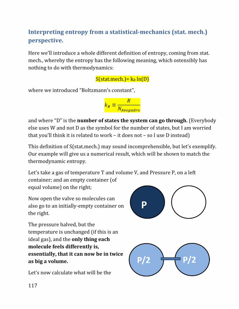
117
Interpreting entropy from a statistical-mechanics (stat. mech.)
perspective.
Here we’ll introduce a whole different definition of entropy, coming from stat.
mech., whereby the entropy has the following meaning, which ostensibly has
nothing to do with thermodynamics:
S(stat.mech.)= kB ln(D)
where we introduced “Boltzmann’s constant”,
�Ú ≡ E³Ù�Å�àÄÅ
and where “D” is the number of states the system can go through. (Everybody
else uses W and not D as the symbol for the number of states, but I am worried
that you’ll think it is related to work – it does not – so I use D instead)
This definition of S(stat.mech.) may sound incomprehensible, but let’s exemplify.
Our example will give us a numerical result, which will be shown to match the
thermodynamic entropy.
Let’s take a gas of temperature T and volume V, and Pressure P, on a left
container; and an empty container (of
equal volume) on the right;
Now open the valve so molecules can
also go to an initially-empty container on
the right.
The pressure halved, but the
temperature is unchanged (if this is an
ideal gas), and the only thing each
molecule feels differently is,
essentially, that it can now be in twice
as big a volume.
Let’s now calculate what will be the

118
increase in the stat. mech. entropy, and verify that it will be exactly what
thermodynamics predicts – so thermodynamics and stat. mech. match (at least
for this case – for a general proof see 110B).
Take a single molecule; its velocity, position within the sphere, internal
vibration, etc. are all things that do not change when the molecule can share its
time between the spheres. So we won’t considered them (we are interested in
changes in the number of states, which will lead to entropy difference, much
more than we care about the total number of states, so we’ll only consider the
new feature, being on the left or right).
So: the new “state” (really “label”) each molecule can be in is only whether it is
left (L) or right (R).
So we can label this “extra” molecular label or state as L or R, and the number of
states for a single molecule is 2.
Now consider 2 molecules; we have LL (two molecules on left), LR, RL, and RR.
Overall 4 states (4=22)
Now 3 molecules: there are 23=8 possibilities: LLL, LLR, LRL, LRR, RLL, RLR,
RRL, RRR
And in general for N molecules, D=2N possibilities.
So if we have “n” moles, they contain N=n*NAvog molecules; so the change in
entropy will be:
S(stat.mech))=kBln(2N),
and using
ln(xy)=yln(x)
we get
S(stat.mech.)= kBN ln(2),
and since
kB *N= (R/NAvog)*(n NAvog)=n R
119
we get
S(stat.mech.)= nR ln(2).
Now this is really not the total stat. mech. entropy, just the change when we
expanded the gas, so we should add a “Delta”, i.e.,
∆∆∆∆S(stat.mech.)= nR ln(2).
Next let’s compare it to the thermodynamics prediction; in thermodynamics,
when a gas is isothermally expanded:
∆∆∆∆S(thermodynamics)= nR ln(Vfinal/Vinitial) (look at the formulae we
derived earlier) i.e., here, when the volume is doubled (and the temperature
unchanged):
∆∆∆∆S(thermodynamics)= nR ln(2V/V)= nR ln(2) = ∆∆∆∆S(stat.mech.) !!
So the two formulations agree, at least for this case.
END OF STAT. MECH., BACK TO THERMODYNAMICS

120
Entropy tabulation and qualitative consideration:
From tables we can determine 0S∆ , change in entropy upon reaction.
Example:
2 2 2( ) 2 ( ) 2 ( )N g O g NO g+ →
Each species contributes to the entropy, with a coefficient that’s the same as in
the reaction, but reactants get a minus
(as ∆S is figuratively products-reactants)
0 0 0 02 2 2( ) 2 ( ) 2 ( )m m mS S N S O S NO∆ = − − +
Where the 0 superscript indicates we calculate at 1 bar.
From tables we find that:
0 J J J J191 2 205 2 240 121
K mol K mol K mol K molS∆ = − − • + • = −
SIDE_NOTE: Note that the entropy is reduced in this reaction
Figuratively, we can understand the entropy reduction, since this reaction
reduces the number of molecules (3 molecules become 2) so there is less
disorder as there are less molecules to roam around.
There are of course complications in reality, but this is a reasonable qualitative
explanation for the entropy reduction.
END OF SIDE NOTE

121
Part 7: Gibbs Free Energy
Summary:
i. Clausius relation: fixed T Δ ����������� . d �� and q≤q(rev.)=TΔ .
ii. Gibbs free energy G=H-TS;
Proof that at fixed P and T, and no electrical workΔ� ≤ 0, and
implications
iii. Predicting transition temperatures *o
o
HT
S
∆=
∆
iv. (dG/dT)P fixed = -S
v. G vs. T diagram at fixed P, stable phase at T,P: lowest G.
vi. Incorporating electrical work Δ� ≤ �Çâ at fixed, T, P
Overview:
We learned that we can see if a process is spontaneous or is reversible according
to the change of entropy in the world:
(world) 0 spontaneous (irreversible)
(world) 0 reversible
(world) 0 forbidden
S
S
S
∆ > →
∆ = →
∆ < →
But it is inconvenient to talk about the change of entropy of the whole world.
Luckily, we can define a new quantity, the Gibbs free energy:
G H TS= −
Such that in the crucial case of reactions at fixed T and P (e.g., bench
experiments in a lab), G will give us the same information as S(world) will
(although with a reverse of signs), i.e.,

122
FOR FIXED P, T (and an assumption we’ll relax later: no electrical work):
0 spontaneous (irreversible)
0 reversible
0 forbidden
G
G
G
∆ < →
∆ = →
∆ > →
Let’s prove.
7.i) Reversible and irreversible for the environment, Clausius
relation
For simplicity, in all the discussion below, the pressure is fixed and the
temperature is fixed.
First, let’s refine our understating of what reversible and irreversible mean as
far as system and as far as surroundings;.
Imagine, e.g., a little balloon containing hydrogen and oxygen and placed in a
pool of fixed temperature
Then, have the hydrogen react with the oxygen to produce water (e.g., maybe
put there a metal that will help catalyze the reaction). As far as the system is
concerned, this is definitely an irreversible process – we cannot do a small
change to make from water back again H and O. (We could put a lot of electricity
to do that, but that’s not a small change).
However, since this is all done in a balloon “immersed” in a pool of fixed
temperature, then, as far as the surroundings are concerned, all that happened
was that the materials in the balloon gave away to the surroundings some heat,
which barely affected the surroundings (maybe very slightly raised the
temperature of the surrounding water).
So: while in the system the process is irreversible, as far as the surrounding all
processes look reversible!
So, if we label the heat given in a process as q, this heat is taken from the
surrounding, so we can say that –q was given to the surrounding
123
(e.g., 10J given to the system is -10J given to the surroundings).
Then:
( .)q H
S surrT T
∆∆ = − = −
where the 2nd equality is since we consider fixed pressures.
(Note that we don’t have this rule for the system: if the process is irreversible,
( .) for irreversible processes)q
S sysT
∆ ≠
Possible values of the heat.
There is a very interesting point “buried” in the derivation above.
This point is called the “Clausius rule”.
The point is that
0 ≤ ∆ *_W9^O& . ∆ + ∆ *NX99& . ∆ – åD . å*9P�. &D – åDwhere the last equality is since we consider a fixed T processes.
So we get:
0 ≤q(rev.)-q i.e.,
å ≤ å*9P�. & *Clausius rule&Clausius rule&Clausius rule&Clausius rule& or equivalently, since ∆S=q*rev.&/T,
å ≤ D ∆ I.e., for any process, reversible or not, the amount of heat input to the system is limited to be less than the amount of heat which will be input in a reversible process.

124
INSERT ExampleExampleExampleExample for Clausius rule for Clausius rule for Clausius rule for Clausius rule ****required, required, required, required, not covered in class¬ covered in class¬ covered in class¬ covered in class&:::: Say we’re at 300K and we start at state I *e.g., a liquid phase of a compound, or a gas at a given volume, or anything else&; and we do a process *expansion, melting, reaction, or something else& that changes the system to a different state, II, with S higher by 4J/K, i.e., ∆S=4J/K. Assume the process is such that the surroundings are at constant temperature; for example, they could be a very large water container into which we “drop” the system. Question: Now let’s pose the hypothetical question: is it possible to do that
same process with (a) q=0; or (b) q=900J; or (c) q=1200J; or (d) q=1500J; and in
every case, will the process be reversible, irreversible, or impossible, and why.
Answer:
(a) q=0 : that means the process was adiabatic. It was irreversible, since
the entropy of the surroundings did not change (they did not give heat),
while the systems’ entropy increases, so the world entropy increases,
i.e., the process is irreversible. An example we discussed is a rapid
adiabatic expansion of a gas without doing work, e.g., when we rupture
the separation between a container full of gas and an initially empty
(“vacuum”) 2nd container, so the gas expands irreversibly from the
initial container to the total final volume (encompassing both
containers).
(b) q=900J. In that case, the surroundings gave away q, (i.e., “got –q” heat)
and since as far as the surroundings this looks reversible, the surr.
entropy change is –q/T, i.e.,
∆S(surr.)= -q/T.-900J/300K = -3J/K So ∆S*world&= ∆S+∆S*surr.&= 4J/K + *-3J/K& = 1 J/K > 0
So the process is possible but again irreversible, since the entropy of the world increases.

125
(c) q=1200J � ∆S(surr.)= -q/T=-1200J/300K = -4J/K
So ∆S*world&= 4 J/K - 4J/K = 0 So the process is reversible *as it does not change the entropy of the world, so in principle we could reverse it&
(d) Finally, the most interesting part:
q=1500J � ∆S*surr.&= -q/T=-1500J/300K = -5J/K So ∆S*world&= 4 J/K - 5 J/K = -J/K So the process is impossible. The reason is it impossible is that when we inject heat into the system we reduce the entropy of the surroundings, and we cannot reduce it by more than 4 J/K, i.e., q needs to be smaller than q*rev.&
ENENENENDDDD OF IN OF IN OF IN OF INSSSSERT EXAMPLE ON CLAERT EXAMPLE ON CLAERT EXAMPLE ON CLAERT EXAMPLE ON CLAUSUSUSUSIIIIUSUSUSUS R R R RUUUULELELELE

126
7.ii) NOW BACK TO DERIVING THE FREE ENERGY AND
IMPLICATIONS
Using the equations above, we get (because we assume that the initial and final
state are at the same temperature and pressure – which is always fixed here, and
the surroundings are at the fixed T and P):
First, assume that there is no electrical work (we’ll relax this later). Since
the pressure is fixed,
( )
( ) ( .)
Rearrange to give:
( )
HS world S S surr S
T
H T SS world
T
∆∆ = ∆ + ∆ = ∆ −
∆ − ∆∆ = −
Now at fixed temperature, a change in G is
( ) ( )G H TS H TS H T S∆ = ∆ − = ∆ − ∆ = ∆ − ∆
(where the 2nd equality is since T is fixed), so that (only at fixed T and P):
( ) (if T,P are fixed)G
S worldT
∆∆ = −
Note: on the left we have a “world” quantity, hard to find;
on the right a system quantity, G∆ , much easier to find.
Since the entropy of the world never decreases, -∆G never becomes negative, i.e.:
0 (if T,P are fixed G never decreases!)G∆ ≤
Very convenient way to know if a process is spontaneous, reversible or
forbidden – since G is a system’s quantity! We don’t have to worry anymore (as
long as we consider processes at fixed T and P) about “world” quantities, only
system quantities!
Example
127
C6H6(l) � C6H6(g), 1atm, 298K.
At 298K, 1atm (we’ll use a 0 superscript, i.e., an umlaut, to denote a quantity
calculated for 1 bar), you can calculate from the information at the appendix of
the book that the reaction enthalpy and entropy is:
( )06 6 6 6( ) ( ) 33.9
mol
kJH H C H l C H g∆ = ∆ → =
0 J kJ96.4 0.0964
K mol K molS∆ = =
Therefore:
0 0 0 kJ kJ kJ33.9 298K 0.0964 5.17 0
mol K mol molG H T S∆ = ∆ − ∆ = − • = >
Therefore, at room temperature and pressure, G 0o∆ > , so the reactant side is
favored, i.e., benzene is a liquid at room temperature and pressure (as we
know!)
128
7.iii) Predicting transition temperature
Let’s say we know at a given temperature what 0 0,H S∆ ∆ are. We can
approximate that they usually don’t change much with temperature (we could
find their exact temperature dependence, from what we know already, based on
the heat capacities, but usually this change with T is relatively small so it can be
ignored in many cases).
Then, we can predict the transition temperature, T*, where the reactants and
products are both allowed, since then ( *) 0G T∆ = :
So:
*o
o
HT
S
∆=
∆
(Of course, this expression predicts that transition never happens if ,o o
H S∆ ∆
don’t have the same sign).
In the Benzene example: 33.9 kJ/mol
* 353K=80 0.0964 kJ/mol
o
o
HT C
S
∆= = = °
∆.
True value: 80.1 C° – excellent agreement! (actually, that’s a little of a
coincidence, usually the agreement is not as good as in this case).
0 ( *) *o oG T H T S= ∆ = ∆ − ∆
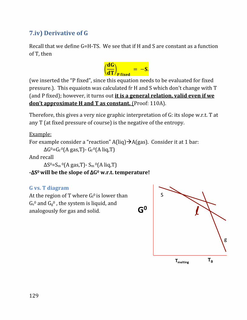
129
7.iv) Derivative of G
Recall that we define G=H-TS. We see that if H and S are constant as a function
of T, then
������ !"zy� . d#.(we inserted the “P fixed”, since this equation needs to be evaluated for fixed
pressure.). This equaiotn was calculated fr H and S which don’t change with T
(and P fixed); however, it turns out it is a general relation, valid even if we
don’t approximate H and T as constant. (Proof: 110A).
Therefore, this gives a very nice graphic interpretation of G: its slope w.r.t. T at
any T (at fixed pressure of course) is the negative of the entropy.
Example:
For example consider a “reaction” A(liq)�A(gas). Consider it at 1 bar:
∆G0=Gf 0(A gas,T)- Gf
0(A liq,T)
And recall
∆S0=Sm 0(A gas,T)- Sm
0(A liq,T)
-∆∆∆∆S0 will be the slope of ∆∆∆∆G0 w.r.t. temperature!
G vs. T diagram
At the region of T where Gl0 is lower than
Gs0 and Gg
0 , the system is liquid, and
analogously for gas and solid.

130
7.v) G AND BATTERIES:
∆G also tells you something very important: how much electrical energy you can
get out of a reaction (or needs to make a reaction happen). Recall that without
electrical work, we derived that
�� � 0*D, 4YWANR. , AWP^PYR9QY8^_W9�&
It turns out (a few lines derivation, see 110A if you take that course), that when
we allow electrical work input or output, then
�� � O_*P^PY. &*D, 4YWANR. &
Integrate, get
$% � w(elec.) (const. T and P only)
EXAMPLES:
Left: G(final) is higher than G(initial) by 5kJ/mol; this means that
�G = 5 kJ/mol, we need to inject at least 5kJ of electrical energy to enable one
mole to react. Without electrical energy, this reaction won’t happen.
Right: G(final) lower than G(initial) by 3kJ/mol – we could use this G difference
to get 3kJ of electrical work from this reaction (for one mole). If reaction is
allowed to happen without extracting the electrical energy, this 3kJ/mol will be
“wasted”, i.e., turn to extra heat.

131
Part 8: Chemical Equilibrium and law of mass action.
Summary: Getting reactions from &% . ëú'÷(búðúûöúbì using a proof that
&% . &%) + tuð'*, ë . &%) + tuð'+
i. Deriving G for an ideal gas:
�U*D, 4& . �U5 *D& + ED � 445�
and mentioning the analogy for solutions:
�U,Ù*îãñ, D& . �U,Ù5 + ED^A |îãñ1T}
i. Reactions and deriving Q
ii. Evolution of Q to K=Qeq
iii. The mass reaction law K and Kc
iv. Properties of K – derived from Kc

132
Law of mass action and Q.
We will derive two major relations in this chapter, which are essentially (once
we understand the meaning of the symbols Q and K) the law of mass action:
∆∆∆∆G = ∆∆∆∆G0 + RT ln(Q)
0000 = ∆∆∆∆G0 + RT ln(K)
The book starts from law of mass action; instead, we will derive it. The
approach we’ll take is to derive a relation between Pj’s in a reaction and ∆∆∆∆G
and use it to get relations about what happens on the way to and in
equilibrium.
The key will be to realize that ∆∆∆∆G=0 in equilibrium, and use it, as well as the
relations between G of a substance and that same substance in a “standard
state”, to get the densities in equilibrium.
(8.ii) G for ideal gas: pressure dependence
We first need the dependence of the molar Gibbs free energy, Gm on
pressure or density, at a fixed temperature.
Three possibilities:
• Solids and liquids: G essentially independent of pressure (at least for our
purposes here), so �U,Ù ≅ �U,Ù5 *D&, where 0 refers to calculation at 1bar, m
denotes molar, and A is a superscript
• Vapors (gases): at a fixed T, G depends on pressure since the entropy
depends on the pressure. Recall that for an isothermal expansion of an ideal
gas, we proved that (see middle of Part 6):
U*D, 4& . U5 *D& d E ln � 445�

133
• Further, the energy of an ideal gas is independent of pressure at fixed T , and
since H=U(T)+PV= U(T)+nRT the enthalpy is also independent of pressure,
i.e., H=H(T) for an ideal gas (and we often label it with a 1bar superscript, as
H=H0(T), even though it is the same at other pressures).
Taken together we get for G of an ideal gas
�U*D, 4& . ,¨5*D& d D U*D, 4&- . |¨5*D& d D � U5 *D& d E ln � 445��}
i.e.,
�U*D, 4& . �U5 *D& + ED � 445� *idealgasonly!&
where:
�U5 *D& ≡ �U*D, 45& . *¨5*D& d D U5 & • Solutions: Finally, consider solutions, i.e., a species “A” in a solution, with a
concentration [A] (for me concentration means molar density, and will be
measured usually in mol/Liter). The Gibbs free energy is dependent on the
concentration, and can be related to a reference concentration (1 M =
1mol/L) as:
�U,Ù*îãñ, D& . �U,Ù5 + ED^A |îãñ1T}*solutions, approximate&
where the zeroth-order Gibbs free energy is now defined NOT with respect to
pressure (the solution’s internal properties do not depend much on external
pressure) but with respect to the reference density,
�U,Ù5 . �U,Ù*1T, D&. Note that the dependence on concentration looks almost the same as the
dependence on pressure of a gas (here the concentration of the solute is
analogous to the pressure of the gas, and the reference concentration, 1M =
1mol/Liter, is analogous to the reference pressure 1bar. This relation is no
coincidence, as we will see later in Section 12 on Raul’s law.
134
(8.iii) Reactions and deriving Q
Now that we have the dependence of G, let’s put it together.
For simplicity, consider a “generic” reaction (actual examples follow later):
3ã*[& + 2á*N& → ãá*[& + ã�á*8å. &
And consider a fixed T (all quantities depend on T, we’ll often hide this
dependence in the derivation to avoid excessive writing).
We know that
Δ� . �U*ãá*[&& + �U,ã�á*8å. &- − 3�U,ã*[&- − 2�U*á*N&&
Of these terms:
• the G of the gases (A, AB) depend on ln of the pressure, e.g.,
�U*ãá& . �UÅ *ãá& + ED ln �4ÙÚ4Å �
• and for the solution (A2B) G depends on ln of the density,
�U,ã�á*NW^. &- = �UÅ *ã�á& + ED ln |îã�á*8å. &ñ1M }
• While the Gm of the solid is independent of pressure
�U,á*N&- . �UÅ *á*N&&
so we get
�� . �UÅ *ãá& + ED ln �4ÙÚ4Å � + �UÅ *ã�á& + ED ln |îã�á*8å. &ñ1M }− 3 ��U5 *ã& + ED ln �4Ù45�� − 2�UÅ *á&
So collecting the G0 terms, we get (very important for the rest of the course!)
�� . ��5 + ED ln.

135
Where
��5 . �UÅ *ãá& + �UÅ *ã�á& d 3�U5 *ã& d 2�UÅ *á& and we defined the reaction quotient, which is here defined as
ln. = ln �4ÙÚ4Å � + ln |îã�á*8å. &ñ1M } − 3 ln �4Ù45�
To develop the ln terms further, recall that
ln e87i = ln*8& − ln*7&
8 ln*7& = ln*7à&
d8 ln*7& = ln � 17à�
So
ln. = ln �eîÙ©Úñ�f i e�Üß�� i
e�Ü��i, §
i.e., here
. . eîÙ©Úñ�f i e�Üß�� ie�Ü��i,
Note: the solid does not enter into Q, since its density does not change (and
therefore its Gibbs free energy does not change.
The same considerations apply to any other reaction; for example, in the
reaction 3NO(g)� NO2(g)+N2O(g), then the same relation (�� . ��5 + ED ln.&
applies, where now

136
2 2
3
NO N O
o o
NOo
P P
P PQ
P
P
=
Another important thing to note about Q is that it is defined always, even if the
reaction did not reach equilibrium; i.e., if we inject NO to a container which is
initially empty, then initially Q will be zero (as N2O and NO2 are initially zero)
but as time passes some NO2 and some NO2 will be made, so Q will grow, until
there is equilibrium, and then Q does not change anymore (since the pressures
of NO, NO2 and N2O will not change anymore). More on this later (we first need
to understand the equilibrium case)
(8.iv) Evolution of Q to K=Qeq.
At the end of the reaction �� . 0, i.e., we reach equilibrium.
The value of Q at equilibrium, is a very special quantity, which we call
� ≡ .*På. &
K has no relation to K used for Kelvin! Just an unfortunate coincidence of
using the same symbol to denote several different things! (Just like we use
P for probability and pressure…)
Since �� . 0at equilibrium,
0 . ��*På. & = ��5 + EDln*.*På. &
i.e.,
0 . ��Š+ ED ln �
So

137
� . exp|d��5ED }
We’ll spend the next few lessons discussing K; but before we do that, let’s
conclude with the more general quantity, Q (recall: K is the equilibrium
value of Q).
Q yields $% and therefore the electric work needed or extractable from the
reaction.
For a general reaction,
Reactants �� products
Depending on the initial condition, if we have too much products or too much
reactants, Q will be larger or smaller than its final value, K (i.e., the
equilibrium value):
If Q is too small initially, then the reaction will shift to the right, i.e.,
products will be made;
Q(t)<K ���� products rise.
If Q is too large initially, then the reaction will shift to the left, reactants
will be made at the expense of the products.
Q(t)>K ���� reactants rise, products lost.
Q can have any value from 0 to infinity. As the graph shows, Q will evolve in
time until it reaches the equilibrium. value, K (which is Temperature-
dependent).
We reemphasize that Q is
related to the amount
of electric work, d&%, that can be extracted
from the reaction:

138
0
/
ln
From def. of K, get:
- ln ln
So:
ln( / )
Divide by RT and expontentiate:
G RT
G G RT Q
RT K RT Q
RT Q K
Qe
G
K
G
∆
∆ = ∆ +
∆
∆
= +
=
=
Note that at late times, when equilibrium is established so Q=K, the overall
difference in Gibbs free energy, G∆ , vanishes, so no more electrical work can be
extracted.
Of course, the change of Q in time does not affect the value of 0G∆ which refers to
what happens when products and reactants are at 1 bar, so it ( 0G∆ ) does not
change in time.
From now one we’ll mostly concentrate on equilibrium (i.e., on K(T)) , mention
Q sporadically, until we get to electrochemistry (batteries) where Q determines
the potential in the battery.
(8.v) The mass reaction law, K and KC
In the remainder of the chapter we will relate K to the mass reaction law as
presented in the book. Further, we will get some properties of K. The next
section, LeChatelier's principle, will allow us to learn how to use K in specific
examples to predict the equilibrium, changes in it, and the reason for the
direction of the change.
Relating to the mass action law.
Take for concreteness the reaction we considered earlier,
3ã*[& + 2á*N& → ãá*[& + ã�á*NW^. &
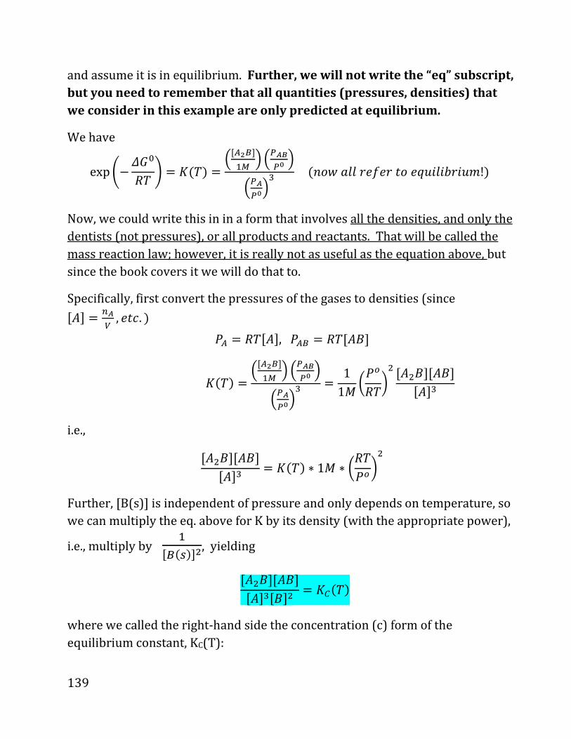
139
and assume it is in equilibrium. Further, we will not write the “eq” subscript,
but you need to remember that all quantities (pressures, densities) that
we consider in this example are only predicted at equilibrium.
We have
exp |−��5ED } = �*D& = eîÙ©Úñ�f i e�Üß�� ie�Ü��i, *AW_8^^9PCP9RWPåXQ^Q79QX�!&
Now, we could write this in in a form that involves all the densities, and only the
dentists (not pressures), or all products and reactants. That will be called the
mass reaction law; however, it is really not as useful as the equation above, but
since the book covers it we will do that to.
Specifically, first convert the pressures of the gases to densities (since îãñ . ÛÜg , PRY. & 4Ù . EDîãñ,4ÙÚ . EDîãáñ �*D& . eîÙ©Úñ�f i e�Üß�� i
e�Ü��i, . 11T �4ÅED�
� îã�áñîãáñîãñ,
i.e.,
îã�áñîãáñîãñ, . �*D& ∗ 1T ∗ �ED4Å��
Further, [B(s)] is independent of pressure and only depends on temperature, so
we can multiply the eq. above for K by its density (with the appropriate power),
i.e., multiply by �îÚ*È&ñ©, yielding
îã�áñîãáñîãñ,îáñ� . �/*D&
where we called the right-hand side the concentration (c) form of the
equilibrium constant, KC(T):

140
�/*D& . 1îá*N&ñ� ∗ 1T ∗ �ED4Å�� ∗ �*D&
The nice thing about �/*D& in the emphasized equation (in blue) is that it is
looks very symmetrical; it has all the densities, and each density is multiplied or
divided and is to the power of its stoichiometric coefficient.
Obviously, we can have such an equation for any reaction, i.e., for a general
reaction
8ã + 7á + Y¬ ↔ Ð + S0 + ó1
We can write
�/*D& . îÐñ�î0ñ�î1ñ�îãñàîáñÆî¬ñ�
regardless if the compounds are gases, liquids, etc., and can relate Kc to K and
therefore to ��. This also makes it easier to derive some properties. However,
you should remember that �� is related to K , not to Kc
(8.vi) Properties of K – derived from Kc
We will use Kc here, but these properties also apply to K
Consider the reaction
aA+bB xX⇔
With
[ ]( )
[ ] [ ]
x
c a b
XK T
A B=
• Reverse reaction – invert K
Now consider the reverse reaction
xX aA+bB⇔
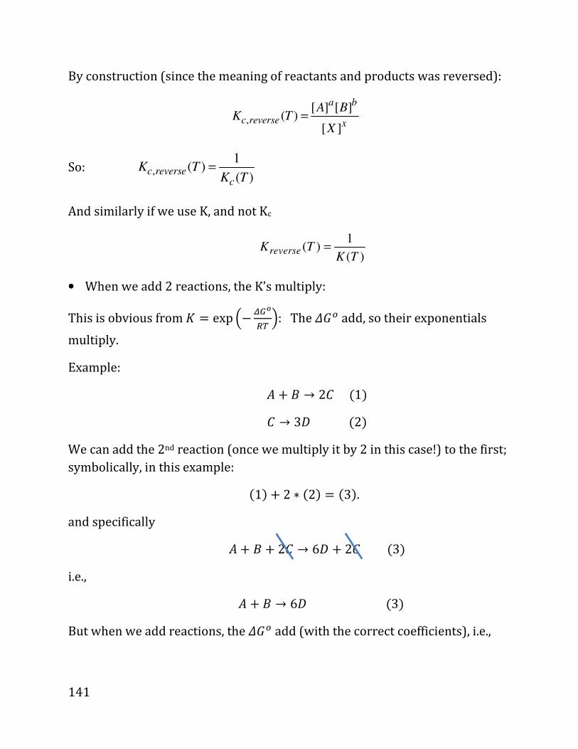
141
By construction (since the meaning of reactants and products was reversed):
,[ ] [ ]
( )[ ]
a b
c reverse x
A BK T
X=
So: ,1
( )( )
c reversec
K TK T
=
And similarly if we use K, and not Kc
1( )
( )reverseK T
K T=
• When we add 2 reactions, the K’s multiply:
This is obvious from � . exp e− 23Þª� i: The ��Å add, so their exponentials
multiply.
Example:
ã + á → 2¬*1&
¬ → 34*2&
We can add the 2nd reaction (once we multiply it by 2 in this case!) to the first;
symbolically, in this example:
*1& + 2 ∗ *2& . *3&. and specifically
ã + á + 2¬ → 64 + 2¬*3& i.e.,
ã + á → 64*3&
But when we add reactions, the ��Šadd (with the correct coefficients), i.e.,
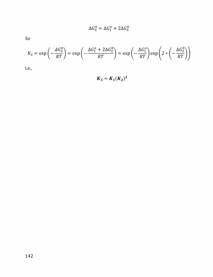
142
Δ�,5 . Δ��Å + 2Δ��5
So
�, . exp |−��,5ED } = exp |−Δ��Å + 2Δ��5ED } = exp |−Δ��ÅED } exp52 ∗ |−Δ��5ED }6
i.e.,
+w . +ê*+x&x
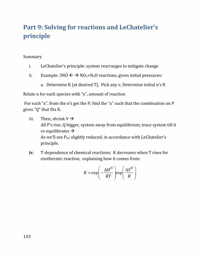
143
Part 9: Solving for reactions and LeChatelier’s
principle
Summary
i. LeChatelier’s principle: system rearranges to mitigate change
ii. Example: 3NO � � NO2+N2O reactions, given initial pressures:
a. Determine K (at desired T), Pick any v, Determine initial n’s R
Relate n for each species with “x”, amount of reaction
For each “x”, from the n’s get the P; find the “x” such that the combination on P
gives “Q” that fits K.
iii. Then, shrink V �
All P’s rise, Q bigger, system away from equilibrium; trace system till it
re-equilibrates �
As we’ll see Ptot slightly reduced, in accordance with LeChatelier’s
principle.
iv. T-dependence of chemical reactions: K decreases when T rises for
exothermic reaction, explaining how it comes from:
0 0
exp expH S
KRT R
∆ ∆= −
144
LeChatelier's principle: a general principle, mostly (but not
always!) obeyed:
Says:
When a system is in equilibrium, and we change some condition, then the
system “fights back” a little, i.e., rearranges itself to somewhat mitigate the effect
of the change of external conditions;
In short:
Systems act to mitigate change.
Simple example:
Consider a reaction room temperature,
ã → 2á
With K=1 at this temperature. Say we reach equilibrium with PTOT=0.75*P0;
(a) What’s PA, PB
(b) Now we change the external conditions, i.e., reduce the total volume.
The system rearranges, as we’ll see. At the new equilibrium the total
pressure is doubled PTOT = 1.5P0; what’s PA final , PB final, and what’s the
relation to LeChatelier’s principle
Answer (we’ll use units where P0=1 and therefore drop the P0 symbol):
(a)
4Ú�4Ù . � . 1so: 0.75 = 4ÒÅÒ = 4Ù + 4Ú = 4Ú�� + 4Ú = 4Ú� + 4Ú
The solution to this 2nd order equation is 4Ú . 0.5, 4Ù = 0.25, Q. P.,twice as
much B as A.
(b) Now Ptot is higher, so
145
1.5 = 4Ú789:;� + 4Ú789:; .Asimple2ndorderequation, withsolution: 4Ú789:; . d1 + √1 + 4 ∗ 1.52 . 0.82
4Ù<ÑÛàâ . 1.5 − 4Ú = 0.68
Note that now the ratio of B to A is much less than 2 (0.82/0.68=1.2!). The
reason is LeChatelier’s principle: the system tries to act to mitigate the
pressure increase; it can do so by converting some of the B into A, as each
time 2B converts to become a single A, the number of molecules is reduced
by 1, therefore relieving some of the increased pressure.
Details of the pressure mitigation
You may ask: where is the pressure mitigation? We started with 0.75 bar, and
ended with 1.5 bar? What was mitigated?
To answer, realize that we only considered what happened at the end, i.e., at
the initial equilibrium and the final equilibrium.
Let me give you the details on what happened, without showing you how I got
this numbers (you’ll see how to do it in a realistic example, in an insert that
follows). See also figure in the next page or two!
Imagine that we reduced the volume extremely fast, before the system had time
to “act”, i.e., so fast that no reactions happen while we reduced.
Turns out that for our problem, the volume was reduced by a factor of 2.18, i.e.,
the final volume is about 46% of the initial volume.
Then, the individual pressures jump.
We know that P=nRT/V, and, since AÙ, AÚ had no time to change, PV is fixed, the
volume reduction by a factor of 2.18 caused a pressure increase of 2.18, so:
4Ù*justafterpush& . 2.18 ∗ 4Ù*beforepush& = 2.18 ∗ 0.25789 = 0.545 4Ú*justafterpush& . 2.18 ∗ 4Ú*beforepush& = 2.18 ∗ 0.5789 = 1.09So
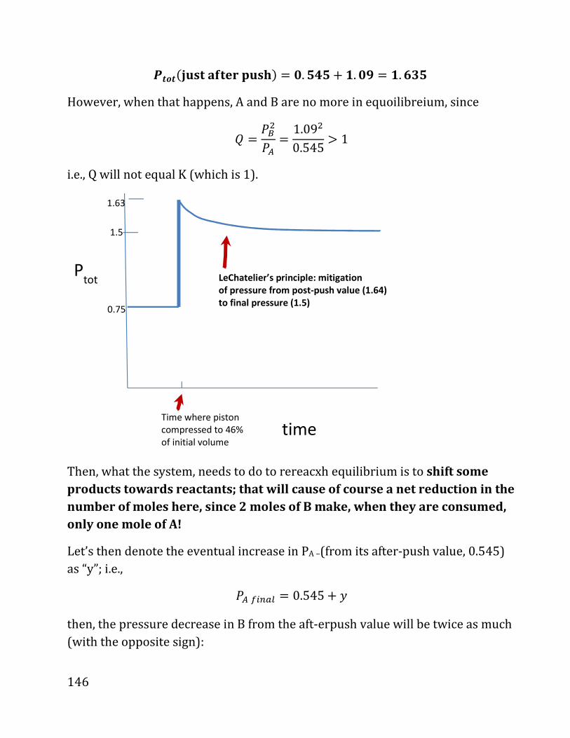
146
ü=)=*>?@AB!AyC{?@D& . ë.EòE + ê. ëF = ê.GwE However, when that happens, A and B are no more in equoilibreium, since
. . 4Ú�4Ù . 1.09�0.545 > 1
i.e., Q will not equal K (which is 1).
Then, what the system, needs to do to rereacxh equilibrium is to shift some
products towards reactants; that will cause of course a net reduction in the
number of moles here, since 2 moles of B make, when they are consumed,
only one mole of A!
Let’s then denote the eventual increase in PA –(from its after-push value, 0.545)
as “y”; i.e.,
4Ù<ÑÛàâ . 0.545 + S
then, the pressure decrease in B from the aft-erpush value will be twice as much
(with the opposite sign):
Ptot
time
Time where piston compressed to 46% of initial volume
0.75
1.63
1.5
LeChatelier’s principle: mitigation
of pressure from post-push value (1.64)
to final pressure (1.5)
147
4Ú789:; . 1.09 − 2S
So then we need to solve:
1 . � . 4Ú<ÑÛàâ�4Ù<ÑÛàâ .
*1.09 − 2S&�0.545 + S . The solution is, as you can verify
S~0.135, so
4Ù789:;~0.68,4Ú789:;~0.82, as we derivd in the beginning.
So to conclude:
• We started with Ptot =0.75, with the system at equilibrium.
• Compressed very quickly reducing the volume by a factor of 2.18 (i.e.,
reducing the total volume to about 46% of its initial value), yileding
Ptot=1.635; that took the system away from equilibrium.
• Then the system rearranges, 2B converts back to A, causing reduction in the
pressure, so Ptot is reduced back to 1.5; this last part is the LeChateliere’s
principle regime – the system fought back a little, and, within the new total
volume (46% of the initial volume), it reached a new equilibrium where the
rise in pressure (from Ptot=0.75 to 1.635 ) is somewhat mitigated, so the final
total pressure is Ptot=1.5
I.e.,
P: 0.75����1.64���� (LeChatelier’s) 1.5.

148
149
INSERT: Comprehensive reliastic example (will teach us about reactions in
general). VERY LONG! NOT COVERED IN CLASS, BUT YOU NEED TO KNOW IT
Take the reaction (all gases)
3NO�� N2O+NO2
at room temperature.
Assume that we do the experiment at 800K, and inject NO and NO2 so that
• the initial pressure of NO is 0.4 bar;
• and the initial pressure of NO2 is 1.6 bar;
• and there’s no N2O initially
Then:
a) Calculate K(T=800K) (don’t get confused between K used for reactions and K
as Kelvin).
b) Calculate the pressures of NO, NO2, N2O in equilibrium, if the total pressure is
kept constant at the same value as it is initially (i.e., Ptot = 2 bar)
c) The next stage will be to increase SUDDENLY the total pressure from 2bar to
4bar and then keep the volume fixed (i.e., shrink the total volume by a factor of
2) calculate the pressures at the new equilibrium (i.e., the equilibrium at the
reduced volume). You’ll see that the new equilibrium is shifted toward s the
products, and this will help to somewhat mitigate the pressure increase
(i.e., the total pressure increased from 2bar to 4bar and is then slightly
reduced).
Answer:
The solution is quite lengthy; we’ll skip over some details.
Schematically:
First determine K;
Then initial pressures (P’s) � initial density (n’s) � vary the density �
determine the pressures and Q � till Q =K.
150
In detail:
(i) First: determining K
K=exp(-∆Go/RT);
The initial temperature is not room temperature; we don’t have ∆Go at that
temperature tabulated.
So to calculate, we’ll have to use
∆Go = ∆Ho - T∆So
We’ll approximate (good enough):
( ) ( )
( ) ( )
0
0
∆ ∆
∆ ∆S
oroom
oroom
H T H T
S T T
≅
≅
so In our case: at room temp., from the table at the end of the book (rounding to
1 significant digit after the period):
( )
( )
2 2
2 2
, , ,
, , ,
kJ – 3 155.4
mol
J kJ – 3 172.1 0.1721
K mol K mol
oroom f NO f N O f NO
oroom m NO m N O m NO
H T H H H
S T S S S
= + = −
= + = − = −
Where in the last part we converted the entropy so it is in kJ/ (mol K), making it
easier to add –TS to H (i.e., ensuring that energy is always in the same unit, kJ).
Next:
0 kJ) 800(800 ) ( ( ) 1
l7.7
mo
o oroom roomG K H T SK T∆ ≅ ∆ ∆ ≅ −− •
so
Also, a useful fact for below is that E ∗ 800� =6.64 kJ/mol (verify!), so
151
�*D . 800�& = exp �− ��ÅE ∗ 800�� . exp �17.7 �¥�¡¢6.64 �¥�¡¢§ = P�.HI = 14.4
(ii) SECOND PART: Determining the pressures, assuming P(total)=2bar
The initial pressures are: (for simplicity we often don’t include the “i" or
“initial;” subscript, but all our results in this subsection are for the initial
pressures and densities).
We need P�n, i.e., the discussion and intermediate formulas should really be
in terms of mole numbers, not pressure.
We know P V= nRT, so, initially:
AB . ?ÑED4B
AB© . ?ÑED4B©
The problem is that we don’t know the initial volume; in essence, we can take
any value of the initial volume, and that will give us a corresponding number
of moles.
Let's take, e.g., Vi=20.75 L (we could have taken any other value, this turns
out to be convenient in the manipulations below). Then:
Using, 1P0*L=100J=0.1kJ, we get
AB . ?ÑED4B . 20.75L ∗ 1.6P¡6.64kJ/mol = 5 P¡LkJ mol = 0.5mol As 4B© . 0.25 ∗ 4B,wegetAB© . 0.25 ∗ AB = 0.125mol (iii) Next, what will happen after the compounds react?
Well, we know the reaction is
3NO(g) �� N2O+NO2

152
That means that when 1 mol of NO2 is made, then 1 mol of N2O will be made, and
3 moles of NO will be consumed; so if an "x" amount of moles is made in the
reaction, then the number of moles of each species will be (we don’t write it
explicitly, but all the densities are in “mol”)
AB . AB*Q& d 3 . 0.5 − 3 AB© . AB©*Q& + . 0.125 +
A©B . A©B*Q& + .
And, as useful for the future:
AÒÅÒ . AB + AB© + A©B . 0.625 −
The allowed values of x are those that lead to non-negative number of moles for
each of the species, i.e., in this case
0 ≤ ≤ 0.53 = 0.1666 (Note that if initially we had all product species, i.e., if N2O was also present, then
"x" could have also been negative).
What's the value of x?
For this we need to go back from densities to pressures.
We are told what's the final pressure, Ptot=2bar, not the final volume; so we use:
4B . ABAÒÅÒ 4ÒÅÒ .0.5 − 30.625 − ∗ 2
Note we calculate all pressures henceforth in units of P0, so we omit the P0
symbol, i.e., Ptot=2, and
4B© . 0.125 + 0.625 − ∗ 24©B . 0.625 − ∗ 2
Now that we have the pressures, we can write Q:
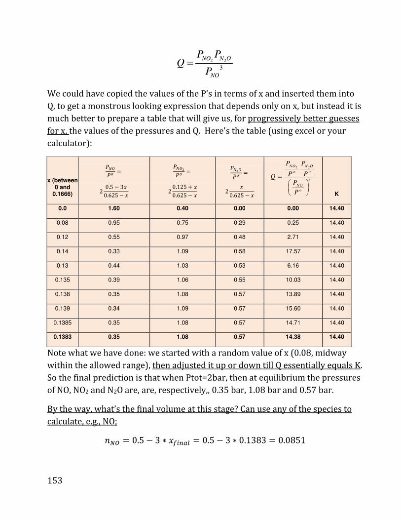
153
2 2
3
NO N O
NO
P PQ
P=
We could have copied the values of the P's in terms of x and inserted them into
Q, to get a monstrous looking expression that depends only on x, but instead it is
much better to prepare a table that will give us, for progressively better guesses
for x, the values of the pressures and Q. Here's the table (using excel or your
calculator):
x (between 0 and
0.1666)
4B4Å . 2 0.5 − 30.625 −
4B©4Å = 2 0.125 + 0.625 −
4©B4Å = 2 0.625 −
2 2
3
o o
NO
NO N
o
OP P
PQP
P
P=
K
0.0 1.60 0.40 0.00 0.00 14.40
0.08 0.95 0.75 0.29 0.25 14.40
0.12 0.55 0.97 0.48 2.71 14.40
0.14 0.33 1.09 0.58 17.57 14.40
0.13 0.44 1.03 0.53 6.16 14.40
0.135 0.39 1.06 0.55 10.03 14.40
0.138 0.35 1.08 0.57 13.89 14.40
0.139 0.34 1.09 0.57 15.60 14.40
0.1385 0.35 1.08 0.57 14.71 14.40
0.1383 0.35 1.08 0.57 14.38 14.40
Note what we have done: we started with a random value of x (0.08, midway
within the allowed range), then adjusted it up or down till Q essentially equals K.
So the final prediction is that when Ptot=2bar, then at equilibrium the pressures
of NO, NO2 and N2O are, are, respectively,, 0.35 bar, 1.08 bar and 0.57 bar.
By the way, what’s the final volume at this stage? Can use any of the species to
calculate, e.g., NO;
AB . 0.5 − 3 ∗ <ÑÛàâ = 0.5 − 3 ∗ 0.1383 = 0.0851
154
?ÇÛÈÒà�ÇÑÑ . EDAB4B . 6640 Jmol ∗ 0.0851mol0.35P¡ . 1615 JP¡ . 16.15L
Of course, we’ll get the same answer if we were to put in the pressure and
number of moles of the other species. Note by way how the final volume in
stage (ii) is smaller than the initial volume we started with (20.75 L); this is
because the reactions reduces here the number of moles, so the same total
pressure is obtained with a smaller volume to accommodate the smaller total
number of moles.
Next part:
(iv) Recall Question (c) from a few pages ago: what happens when we
shrink the resulting system in part ii so that the pressure suddenly
rises from 2bar to 4bar, and then keep the volume fixed.
When we quickly double the pressure, before any reactions happened (it may be
very difficult in practice to do it so quickly, but let’s assume we can shrink it very
fast), then V is shrank by a factor of 2, from Vendof ii = 16.14L to Viii= 8.08L
Then, we need to do a similar table to the one we had before, except that now
we know the volume, not the total pressure. So therefore we use:
ED?ÑÑÑ .6640 J
UÅâ8.08é = 8.21 45�W^ So:
4B . ED?ÑÑÑ AB . 8.21 ⋅ *0.5 − 3& ⋅ 45
And similarly:
4B© . ED?ÑÑÑ AB© . 8.21 ⋅ *0.125 + & ⋅ 4Å , 4©B . ED?ÑÑÑ A©B . 8.21 ⋅ ⋅ 4Å
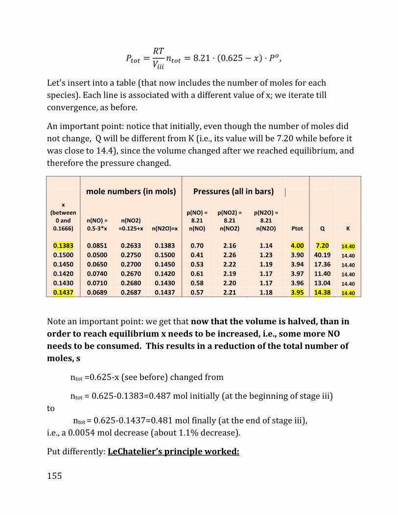
155
4ÒÅÒ . ED?ÑÑÑ AÒÅÒ . 8.21 ⋅ *0.625 − & ⋅ 4Å , Let's insert into a table (that now includes the number of moles for each
species). Each line is associated with a different value of x; we iterate till
convergence, as before.
An important point: notice that initially, even though the number of moles did
not change, Q will be different from K (i.e., its value will be 7.20 while before it
was close to 14.4), since the volume changed after we reached equilibrium, and
therefore the pressure changed.
mole numbers (in mols) Pressures (all in bars)
x
(between
0 and
0.1666)
n(NO) =
0.5-3*x
n(NO2)
=0.125+x n(N2O)=x
p(NO) =
8.21
n(NO)
p(NO2) =
8.21
n(NO2)
p(N2O) =
8.21
n(N2O) Ptot Q K
0.1383 0.0851 0.2633 0.1383 0.70 2.16 1.14 4.00 7.20 14.40
0.1500 0.0500 0.2750 0.1500 0.41 2.26 1.23 3.90 40.19 14.40
0.1450 0.0650 0.2700 0.1450 0.53 2.22 1.19 3.94 17.36 14.40
0.1420 0.0740 0.2670 0.1420 0.61 2.19 1.17 3.97 11.40 14.40
0.1430 0.0710 0.2680 0.1430 0.58 2.20 1.17 3.96 13.04 14.40
0.1437 0.0689 0.2687 0.1437 0.57 2.21 1.18 3.95 14.38 14.40
Note an important point: we get that now that the volume is halved, than in
order to reach equilibrium x needs to be increased, i.e., some more NO
needs to be consumed. This results in a reduction of the total number of
moles, s
ntot =0.625-x (see before) changed from
ntot = 0.625-0.1383=0.487 mol initially (at the beginning of stage iii)
to
ntot = 0.625-0.1437=0.481 mol finally (at the end of stage iii),
i.e., a 0.0054 mol decrease (about 1.1% decrease).
Put differently: LeChatelier’s principle worked:
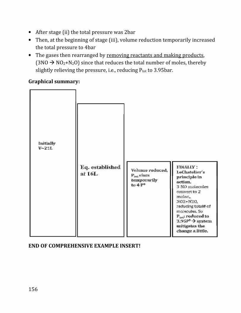
156
• After stage (ii) the total pressure was 2bar
• Then, at the beginning of stage (iii), volume reduction temporarily increased
the total pressure to 4bar
• The gases then rearranged by removing reactants and making products,
(3NO � NO2+N2O) since that reduces the total number of moles, thereby
slightly relieving the pressure, i.e., reducing Ptot to 3.95bar.
Graphical summary:
END OF COMPREHENSIVE EXAMPLE INSERT!
157
LeChatelier’s principle for the T-dependence of
K(T).
Prologue: for pressure LeChatelier's principle implied that a reacting system
fights back a pressure increase by rearranging products or reactants to decrease
the change,
Similarly, for a raise of Temperature a similar phenomenon occurs, as we will
show now – the system rearranges (shifts towards products or reactants) in a
way that will "absorb" some of the extra energies.
In detail: First, recall some definitions.
Reactions with ∆∆∆∆H0<0 are called exothermic; the reaction releases heat. (H
of reactants higher than that of product).
∆∆∆∆H0>0 are called endothermic; the reaction absorb heat from surrounding.
Let’s see the temperature dependence of K and how it relates to LeChatelier’s
principle.
0 0 0 0 0
exp exp expG H RT S H S
KRT RT RT R
∆ ∆ − ∆ ∆ ∆= − = − = − +
Which we’ll write as
0 0
exp expH S
KRT R
∆ ∆= −
Now usually, as mentioned, ∆H0 and ∆S0 don’t change much with temperature,
so the T-dependence of K is due to the 1/T term in 0
expH
RT
∆−
.

158
For an exothermic reaction, ∆H0<0 – Thus, at low temperatures (where 1/T is
very large) 0
H
RT
∆− is very positive,
but when T is larger, 1/T is smaller, so 0
H
RT
∆− is less positive;
In short, for exothermic reactions lnK (and therefore K) decreases with T.
Let’s understand it in terms of LeChatelier’s principle.
For an exothermic reaction, when we raise the temperature, the system wants to
fight this change;
The way to do it is to move products back into reactants, since reactants store
energy in them, i.e.,
By moving products back to reactant the system :
• reduces the kinetic energy (and therefore reduce the temperature) and
• convert it to the potential energy stored by the reactant.
Qualitatively, imagine that we consider
some exothermic reaction, which is at
equilibrium at room temperature; raise
the temperature VERY QUICKLY (before
the system has time to react and change
the number of products and reactant)
In); and then let it evolve;
What LeChatelier’s principle tells you is
that the system will then shift so more products to reactants (reduce # of
products, raise # of reactant' moles), as this will cause the "absorption" of
kinetic energy.

159
Practical calculation of K at different temperatures:
From:
0 0
exp expH S
KRT R
∆ ∆= −
we get:
ln �*D& = −�¨ÅED + � ÅE
Again, approximate that �¨Åand � Å are both T-independent.
We apply this equation at two different temperatures we get
ln �*D�& = −�¨ÅED� + � ÅE
ln �*D�& = −�¨ÅED� + � ÅE
Subtracting gives
ln �*D�& − ^A�*D�& . d �¨ÅED� d ��¨Å
ED� � . d�¨ÅE � 1D� d 1D��
Therefore, from the rate at one temp. and from �¨Å ,the amount of heat given
or taken in the reaction, we can find the rate at other temperature.
160
Part 10: Acids and Bases
Contents:
i) Definitions – acids and bases donate/accept protons; Lewis
definitions; Kw, pH and pKa
ii) Densities when pH is known: Determining neutral/ionic densities of
an acid, [HA] and îã»ñ from pH.
Indicators.
iii) Determining î¨çñwhen we throw into a solution acids/bases.
Buffers.
iv) Determining an unknown amount of an acid: Titrations.
NOTE: THROUGOUT THIS CHAPTER WE’LL ALWAYS REFER TO MOLAR
DENSITIES [A] IN MOLES PER LITER, M, AND WE OFTEN WON’T DESIGNATE
THE UNIT M.
i) Definitions – acids and bases.
Define:
Acid: (Bronsted-Lowry) – Proton Donor
Base (Bronsted-Lowry) – Proton Acceptor
Dissolution in Water:
2 3( .) ( ) ( ) ( .)
( ) (base) (conjugate conjugate
acid) base)
HA aq H O l H O aq A aq
acid
+ −+ ⇔ +
161
Equivalently we write: ( .) ( .) ( .)HA aq H aq A aq+ −⇔ +
Similarly, we write a generic base equation:
2( .) ( ) ( .) ( .)
base acid conj. acid conj. base
B aq H O l BH aq OH aq+ −+ ⇔ +
More generally: + +
acid base base conj.toA acid conj. to B
HA B A BH− +⇔
Note that we don’t need to have a water solution at all, as in the reaction
3 4( ) ( ) ( )HCl g NH g NH Cl s+ ⇔
Since the latter is essentially a ³¨�ç + ¬^» solid; i.e., this reaction shifts ¨ç
from HCl to ³¨�ç
Protons and protonated water:
Note that a proton in water will always get water around it.
2 3
Notation equivalence:
O O +A
means the same as:
+
HA H H
HA H A
+ −
+ −
+ ⇔
⇔
¨,¹ç(aq.) or ¨ç (aq.) are equivalent ways of denoting proton solvated in
water, so we can use 3[ ] [ ]H O H+ += interchangeably.
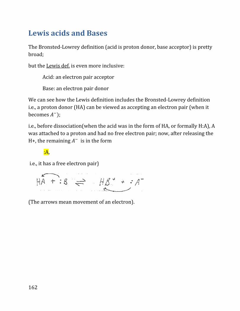
162
Lewis acids and Bases
The Bronsted-Lowrey definition (acid is proton donor, base acceptor) is pretty
broad;
but the Lewis def. is even more inclusive:
Acid: an electron pair acceptor
Base: an electron pair donor
We can see how the Lewis definition includes the Bronsted-Lowrey definition
i.e., a proton donor (HA) can be viewed as accepting an electron pair (when it
becomes ã»&;
i.e., before dissociation(when the acid was in the form of HA, or formally H:A), A
was attached to a proton and had no free electron pair; now, after releasing the
H+, the remaining ã» is in the form
:A,
i.e., it has a free electron pair)
(The arrows mean movement of an electron).

163
Acid examples:
Water:
Note: most are oxyacids (release H bonded to O).
ü∝
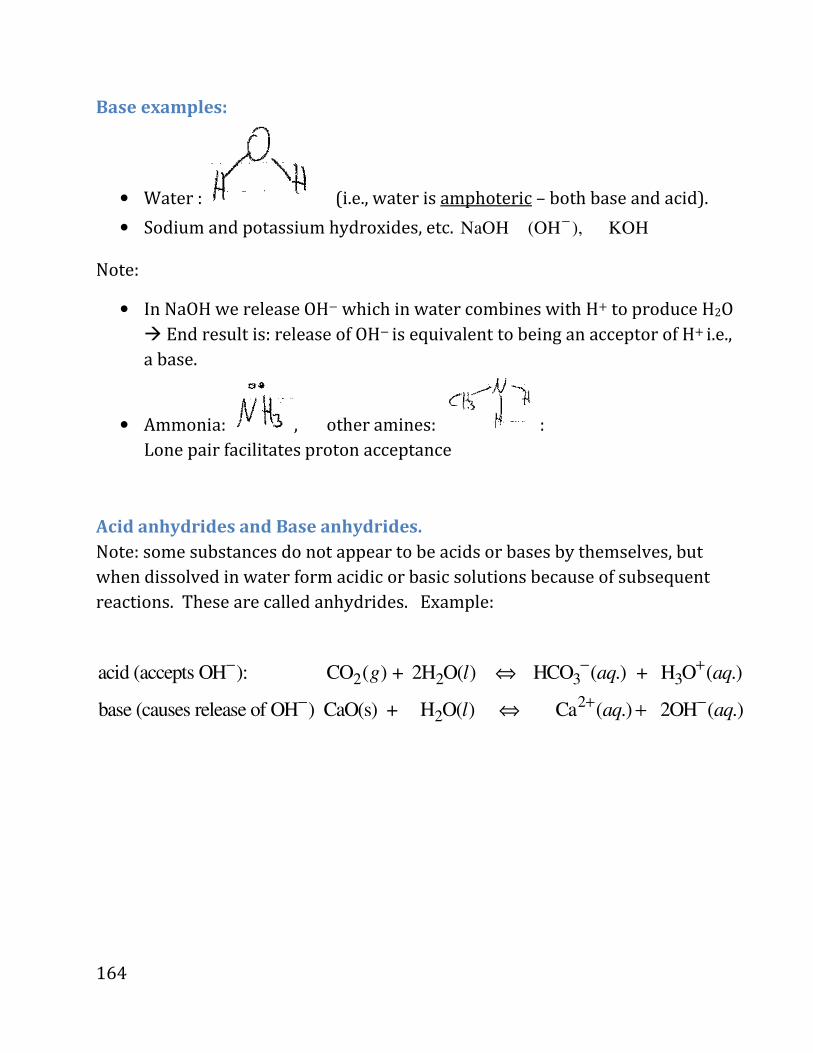
164
Base examples:
• Water : (i.e., water is amphoteric – both base and acid).
• Sodium and potassium hydroxides, etc. NaOH (OH ), KOH−
Note:
• In NaOH we release OHd which in water combines with H+ to produce H2O
� End result is: release of OHd is equivalent to being an acceptor of H+ i.e., a base. • Ammonia: , other amines: :
Lone pair facilitates proton acceptance
Acid anhydrides and Base anhydrides.
Note: some substances do not appear to be acids or bases by themselves, but
when dissolved in water form acidic or basic solutions because of subsequent
reactions. These are called anhydrides. Example:
2 2 3 3
22
acid (accepts OH ): CO ( ) + 2H O( ) HCO ( .) + H O ( .)
base (causes release of OH ) CaO(s) + H O( ) Ca ( .) 2OH ( .)
g l aq aq
l aq aq
− − +
− + −
⇔
⇔ +
165
Acid strength: refers to species ability to donate proton to water:
2 3( .) ( ) ( .) ( .)HA aq H O l H O aq A aq+ −+ ⇔ +
And since it is impossible to designate whether a proton is free (H+) or bound to
water molecule (H3O+), we can rewrite the equation above simply as
( .) ( .) ( .)HA aq H aq A aq+ −⇔ +
Def.:
[ ][ ]
(acid dissoc. const.)=[ ]
A
H AK K
HA
+ −
≡
KA >> 1 � HA is a strong acid.
KA << 1 � HA is a weak acid.
Strong acids: equilibrium in highlighted equation lies to the right �When an
acid HA (initially of concentration [HA]0 ) is poured into water almost all of it
dissociates, i.e., îK»ñ ≅ îLKñë.
Weak acids: equi. is often (some exceptions) far left, îK»ñ ≪ îLKñë but this
depends on 0[HA]
Convenient characterization of strength of acid is pKa,
10log ( )a apK K= −
(Note: acids and bases are the only time in this course where we refer to log10, as
in other places we use ln, i.e., log in base e).
Examples:
7
5
10 7 (strong acid)
10 5 (weak acid)
a a
a a
K pK
K pK−
= → = −
= → =
166
Clearly a species with a more positive pKa will be a weaker acid as its Ka is
lower.
Base Strength
Species ability to snatch proton from water to form OHd(aq.)
2 ( ) ( .) ( .) ( .)
[ ][ ]
[ ]
b
H O l B aq OH aq BH aq
OH BHK K
B
− +
− +
+ ⇔ +
≡ =
And of course:
10log ( )b bpK K= −
Note:
1: bK >> strong base, many OHd produced, little îBñ left. 1: bK << weak base, most [B] remains.
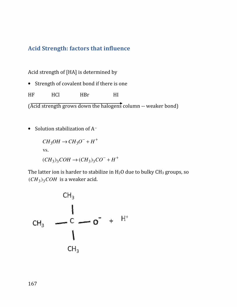
167
Acid Strength: factors that influence
Acid strength of [HA] is determined by
• Strength of covalent bond if there is one
HF HCl HBr HI
(Acid strength grows down the halogens column -- weaker bond)
• Solution stabilization of Ad
3 3
3 3 3 3
vs.
( ) ( )
CH OH CH O H
CH COH CH CO H
− +
− +
→ +
→ +
The latter ion is harder to stabilize in H2O due to bulky CH3 groups, so
3 3( )CH COH is a weaker acid.

168
KW
Water: acts as acid and base, i.e.,
2
2 2 3
( ) ( .) ( .)
( written as ( ) ( ) ( .) ( .))
[ ][ ] W
H O l H aq OH aq
sometimes H O l H O l H O aq OH aq
K H OH
+ −
+ −
+ −
⇔ +
+ ⇔ +
=
Kw(T) : water dissociation constant.
In any aq. solution at equi., ( ) [ ][ ] WK T H OH+ −= is constant, i.e., independent
of everything else except T.
[word of caution – if the solution stops being aqueous solution, i.e., if it is, say,
less than ~ 70% water, the product can change; but we won’t discuss such
situations]
The most important KW is for T=250C: Kw(298K)= 10-14
(not exactly, but very close to this round number; also, KW has units of
M=mol/Liter, so it is really 10-14M2, but we often don’t carry the M units around).
Since in pure water the positive and negative ions have the same conc., than in
pure water: 7[ ] [ ] 10 MH O H
+ − −= =
An aq. solution with [ ] [ ]H OH+ −= is called neutral solution.
Acidic aq. solution has [ ] [ ]H OH+ −>
Basic aq. solution has: [ ] [ ]H OH+ −<
169
Note that the fact that [ ][ ]WK H OH+ −= allows to connect:
• KA for acid HA and
• KB for the conj. base, Ad
Method: Since
( .) ( .) ( .)
[ ][ ]
[ ]a
HA aq H aq A aq
H AK
HA
+ −
+ −
⇔ +
=
and
2
2
( .) ( ) ( .) ( .)
( . ., ( .) ( ) ( .) ( .), where )
[ ][ ]
[ ]b
A aq H O l HA aq OH aq
i e B aq H O l HB aq OH aq B A
HA OHK
A
− −
+ − −
−
−
+ ⇔ +
+ ⇔ + =
=
It follows that:
[ ][ ][ ][ ][ ][ ]
[ ][ ]a b W
H A HA OHK K H OH K
HA A
+ − −+ −
−= = =
The product on the right is just our good old KW ! I.e.,
Wb
a
KK
K=
I.e., if Ka is known ���� find Kb for conj. basis.

170
PH scale:
Acidity quantified by def. of “pH” or “power of hydrogen ion”:
10log [ ]pH H+≡ −
At 25 Celsius:
7
7
7
Neutral: [H ] 10 7
acidic: [H ] 10 7
basic: [H ] 10 7
M pH
M pH
M pH
+ −
+ −
+ −
= → =
> → <
< → >
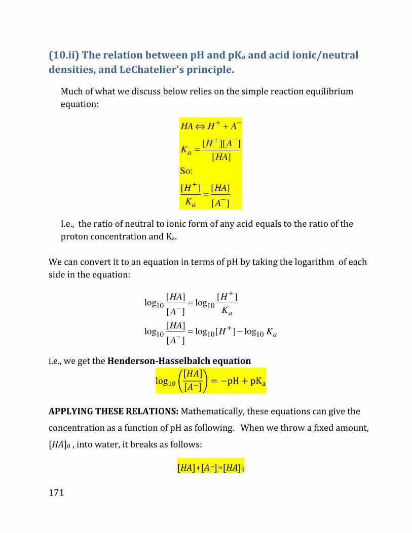
171
(10.ii) The relation between pH and pKa and acid ionic/neutral
densities, and LeChatelier’s principle.
Much of what we discuss below relies on the simple reaction equilibrium
equation:
[ ][ ]
[ ]
So:
[ ] [ ]
[ ]
a
a
HA H A
H AK
HA
H HA
K A
−+
+ −
+
−
⇔ +
=
=
I.e., the ratio of neutral to ionic form of any acid equals to the ratio of the
proton concentration and Ka.
We can convert it to an equation in terms of pH by taking the logarithm of each
side in the equation:
10 10
10 10 10
[ ] [ ]log log
[ ]
[ ]log log [ ] log
[ ]
a
a
HA H
KA
HAH K
A
+
−
−+
=
= −
i.e., we get the Henderson-Hasselbalch equation
log�5 |î¨ãñîã»ñ} = −pH + pKN
APPLYING THESE RELATIONS: Mathematically, these equations can give the
concentration as a function of pH as following. When we throw a fixed amount,
[HA]0 , into water, it breaks as follows:
[HA]+[Ad]=[HA]0
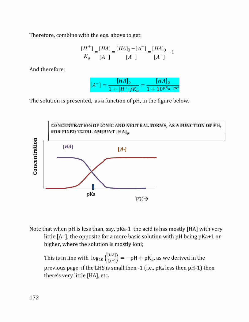
172
Therefore, combine with the eqs. above to get:
0 0[ ] [ ] [ ][ ] [ ]1
[ ] [ ] [ ]a
HA A HAH HA
K A A A
−+
− − −
−= = = −
And therefore:
îã»ñ . î¨ãñ51 + î¨çñ/�à . î¨ãñ51 + 10��:»�@
The solution is presented, as a function of pH, in the figure below.
Note that when pH is less than, say, pKa-1 the acid is has mostly [HA] with very
little îA»ñ; the opposite for a more basic solution with pH being pKa+1 or
higher, where the solution is mostly ioni;
This is in line with log�5 eî@ÙñîÙOñi . dpH + pKN, as we derived in the
previous page; if the LHS is small then -1 (i.e., pKa less then pH-1) then
there’s very little [HA], etc.
173
Side note: LeChatelier’s principle
Note that the 10[ ]
log[ ]
a
HApK pH
A−
= − equation is according to LeChatelier’s
principle: if the equilibrium is shifted so that the solution is more acidic (H+
increases e.g., if another acid is poured in), then the solution will “fight” this
change by decreasing îã»ñ, i.e., shifting some of the protons so that they
react with îã»ñ and make HA. So the more acidic the environment (the
lower the pH), the more neutral the acid; and if the environment is less
acidic, than the acid will ionize.
• Indicators:
From the graph above we see how to determine pH:
Throw in an acid a known pKa that absorbs in different colors in the neutral
[HA] and ionic [ã»ñ forms; if the color is mostly of [HA], then pH>pKa, and
vice versa. If we throw several indicators, each with a different pH, we can
nail the pH fairly accurately – this is how litmus paper works.
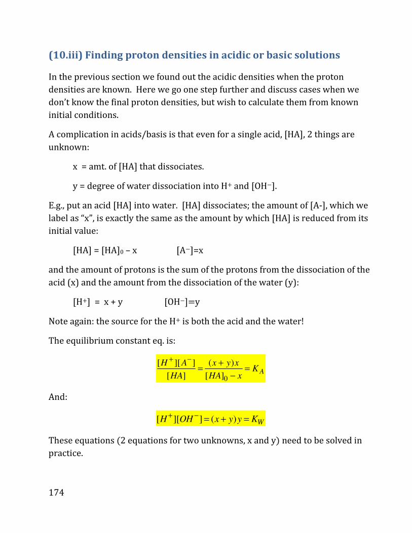
174
(10.iii) Finding proton densities in acidic or basic solutions
In the previous section we found out the acidic densities when the proton
densities are known. Here we go one step further and discuss cases when we
don’t know the final proton densities, but wish to calculate them from known
initial conditions.
A complication in acids/basis is that even for a single acid, [HA], 2 things are
unknown:
x = amt. of [HA] that dissociates.
y = degree of water dissociation into H+ and [OHd].
E.g., put an acid [HA] into water. [HA] dissociates; the amount of [A-], which we
label as “x”, is exactly the same as the amount by which [HA] is reduced from its
initial value:
[HA] = [HA]0 – x [Ad]=x
and the amount of protons is the sum of the protons from the dissociation of the
acid (x) and the amount from the dissociation of the water (y):
[H+] = x + y [OHdñ.y Note again: the source for the H+ is both the acid and the water! The equilibrium constant eq. is:
0
[ ][ ] ( )
[ ] [ ]A
H A x y xK
HA HA x
+ − += =
−
And: [ ][ ] ( ) WH OH x y y K
+ − = + = These equations *2 equations for two unknowns, x and y& need to be solved in practice.
175
Simplification: Strong acids:
Simplification: in strong acids, since there’s “a lot” of [H+], then [OHd] is almost
zero (since the product of these two ions is fixed, i.e., is Kw ).
Therefore, y (i.e., [OHd] ) is almost zero, so we can neglect it relative to x, (i.e.,
we can’t assume that y is zero, but we can assume that x+y equals x) . So we'll
find x first, then y later.
Example: HCl at room temp. where Kcl=107; let’s say that the initial conc. of
[HCl] is 2 (i.e., 2M, i.e., 2mol/L, the unit we are always using)
So: 1410 ( ) ~ i.e.,
~
W
W
K y x y yx
K xy
−= = +
And similarly:
2
7
2
[ ][ ] ( )~
[ ] 2 2
Since large (~10 ),
and the numerator above (x ) cannot be too large,
Then 1/(2-x) must be large, i.e., 2-x is small
so x~2 (not ex
Cl
Cl
H Cl x x y xK
HCl x x
K
+ − += =
− −
=
14 1415
actly, but close to it),
10 10 and =5 10 .
2y
x
− −−≅ ≅ �
So to conclude:
15
7
7
[ ] 2 , [ ] 2 , [OH ] 5 10
[ ][ ] (2 )(2 )[ ] 4 10
10Cl
H M Cl M M
H Cl M MHCl M
K M
+ − − −
+ −−
= = = •
= = = •.
Key point: for all practical purposes, strong acids dissociate completely.
Strong bases: completely analogous.
176
Neutralization:
Say we have solution of strong acid + strong base.
Assume strong acid dissociates completely to H A+ −+
And B similarly dissociates: 2H O B HB OH+ −+ ⇔ +
Physically we know what will happen: the OHd and H+ will neutralize each
other, and the one which has a higher conc. will prevail.
I.e., let’s denote by 0[ ] [ ]H HA+ =
0 the max. conc. of protons (or [H3O+ñ) just due
to dissociations of the acid and similarly define [OHd]0 =[B]0 ; this is before
neutralization of the [OHd] and [H+].
Then, if [H+]0 > [OHd]0 , then almost all the »ñ is neutralized by reactions
with protons, so we can:
* find the remaining [H+],
* and from that we find the small number of »ñ remaining:
0 0
14
[ ] [ ] [ ]
[ ] (so [ ][ ] 10 )[ ]
W
H H OH
KOH H OH
H
+ + −
− + − −+
≅ −
= =
and opposite to this if [H+]0 < [OHd]0 .
EXAMPLE:
1M HCl + 0.4 M NaOH
[H+]0 = 1M, [OHd]0=0.4M �
[H+] = 1M-0.4M=0.6M,
[OHd]=(10-14 M2 / 0.6M) = 1.6*10-14 M
177
Weak acids:
Mathematical solution has to be done explicitly then.
But if pH<5, [H+] >> [OHd], so we can apply similar techniques, i.e., we can
assume that the water isn’t ionized (i.e., in our language, y<<x). (I.e., since the
[OH-] concentration is small, it means that very little [OH-] was produced from
water, i.e., the water was not ionized, the H+ concentration is almost all due to
the acid.)
178
Polyprotic acids: (poly- a lot; protic – proton):
Acids which can lose more than one proton
42 3 3 1
2 113 3 2
K 1.2*10
K 4*10
H CO H HCO
HCO H CO
+ − −
− + − −
→ + =
→ + =
Note that in the first reaction, 3HCO
− has the role of a base (conjugate base),
and in the 2nd reaction it is an acid.
Question:
Say that we pour into water 0.034M H2CO3, which then reacts via the reactions
above;
what’s the concentration of the resulting 3 HCO
− and 2 3 CO
− as a function of
PH?
Answer:
There are 2 ways to answer this.
First, almost blindly following the mathematics. This is done in the book.
Second, a graphical solution.
We know that compound will shed its H when pH starts very low and then
increases past pK1. At a much higher pH, around pK2 the singly ionized
form sheds the 2nd hydrogen. Since pK2 and pK1 are far away, pK2 (here
pK1~3.8; pK2~10.5 ) the polyprotic acids change of distribution as a
function of proton concentration can be viewed as two separate processes.
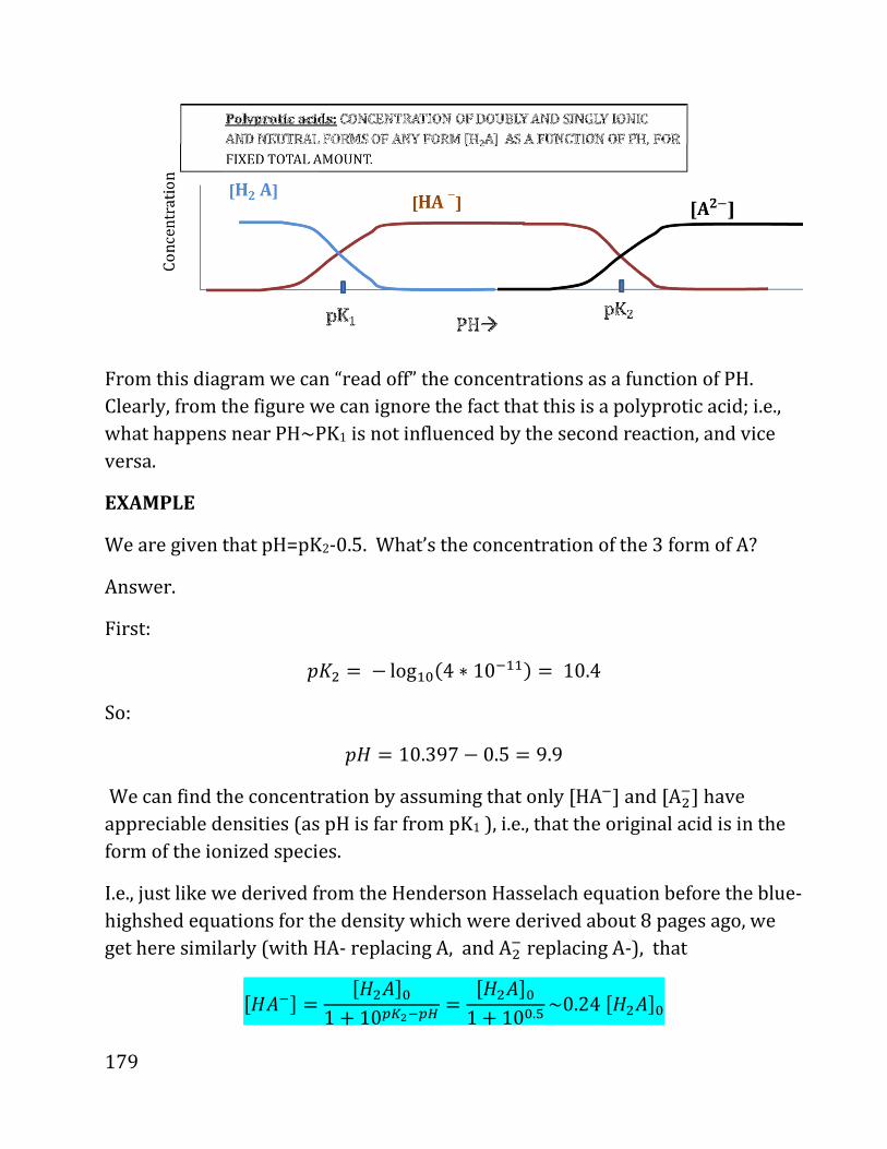
179
From this diagram we can “read off” the concentrations as a function of PH.
Clearly, from the figure we can ignore the fact that this is a polyprotic acid; i.e.,
what happens near PH~PK1 is not influenced by the second reaction, and vice
versa.
EXAMPLE
We are given that pH=pK2-0.5. What’s the concentration of the 3 form of A?
Answer.
First:
]�� .d log�5*4 ∗ 10»��& . 10.4
So:
]¨ . 10.397 − 0.5 . 9.9
We can find the concentration by assuming that only [HA»] and [A�»] have
appreciable densities (as pH is far from pK1 ), i.e., that the original acid is in the
form of the ionized species.
I.e., just like we derived from the Henderson Hasselach equation before the blue-
highshed equations for the density which were derived about 8 pages ago, we
get here similarly (with HA- replacing A, and A�» replacing A-), that
î¨ã»ñ . î¨�ãñ51 + 10��©»�@ . î¨�ãñ51 + 105.Ê~0.24î �̈ãñ5
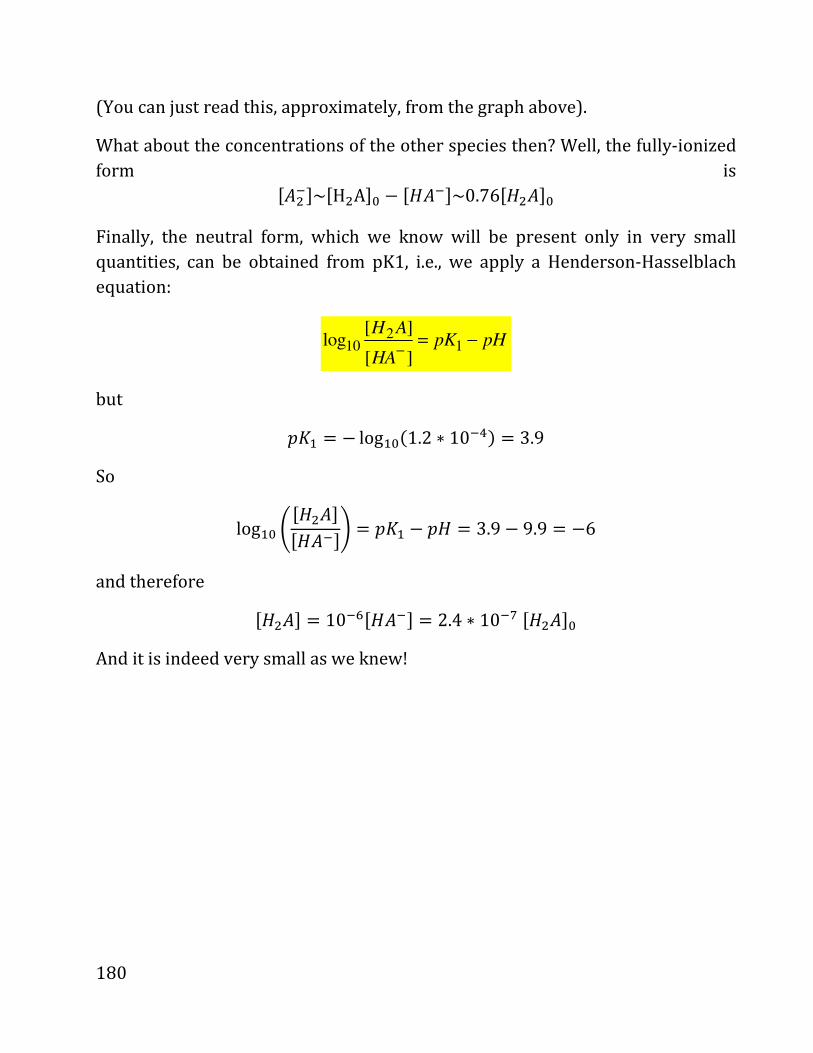
180
(You can just read this, approximately, from the graph above).
What about the concentrations of the other species then? Well, the fully-ionized
form is îã�»ñ~îH�Añ5 − î¨ã»ñ~0.76î¨�ãñ5
Finally, the neutral form, which we know will be present only in very small
quantities, can be obtained from pK1, i.e., we apply a Henderson-Hasselblach
equation:
210 1
[ ]log
[ ]
H ApK pH
HA−
= −
but
]�� . d log�5*1.2 ∗ 10»�& = 3.9
So
log�5 |î¨�ãñî¨ã»ñ} = ]�� − ]¨ = 3.9 − 9.9 = −6
and therefore
î¨�ãñ . 10»Hî¨ã»ñ . 2.4 ∗ 10»Iî¨�ãñ5
And it is indeed very small as we knew!

181
Buffers: Best understood by example:
Without buffers, a little bit of acid can change the acidity wildly.
For example, take 1L of water, neutral – so pH=7. Then, take a small amount,
0.01 mole, of a strong acid added to the water� density is 0.01 m/L = 0.01 M,
pH=-log10(0.01)= 2 � Very acidic (high proton concentration).
Can we find a way to have a weaker acidity, which will be less dependent on
what else happens?
The first key is to invoke the equation as we had before, that says that for any
acid:
[ ][ ]
[ ]a
HAH K
A
+−
=
So if we can find an acid HA such that [ ], [ ]HA A−
can be made to be both
appreciable, then [ ]H+ won’t change much, and will be very close to Ka
(i.e., pH will be close to pKa).
Another way to see it is to remember that:
10[ ]
log[ ]
a
HApK pH
A−
= −
So if î@ÙñîÙOñ is not large nor small (say is between 0.1 and 10), its logarithm will not
be a very big number, and therefore pH will be close to pKa.
The way to assure that
î@ÙñîÙOñ is not too large or small is:
• Put in a specific amount of weak acid, HA with weak base [ ]A− as conjugate.,
and:
• At the same time add a source of the conjugate.
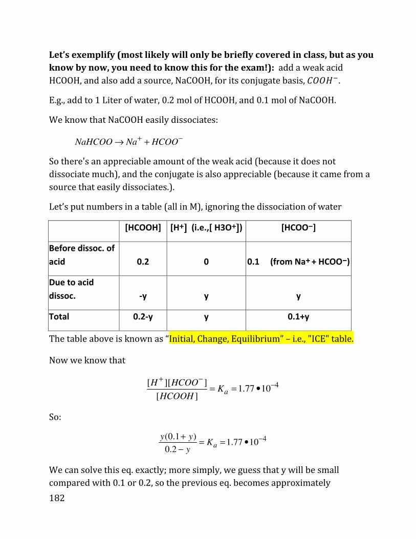
182
Let’s exemplify (most likely will only be briefly covered in class, but as you
know by now, you need to know this for the exam!): add a weak acid
HCOOH, and also add a source, NaCOOH, for its conjugate basis, ¬¹¹¨».
E.g., add to 1 Liter of water, 0.2 mol of HCOOH, and 0.1 mol of NaCOOH.
We know that NaCOOH easily dissociates:
NaHCOO Na HCOO+ −→ +
So there's an appreciable amount of the weak acid (because it does not
dissociate much), and the conjugate is also appreciable (because it came from a
source that easily dissociates.).
Let’s put numbers in a table (all in M), ignoring the dissociation of water
[HCOOH] [H++++ññññ (i.e.,[ H3O++++ññññ) [HCOOdddd]
Before dissoc. of
acid 0.2 0 0.1 (from Na+ + + + + HCOO−−−−)
Due to acid
dissoc. -y y y
Total 0.2-y y 0.1+y
The table above is known as “Initial, Change, Equilibrium” – i.e., "ICE" table.
Now we know that
4[ ][ ]1.77 10
[ ]a
H HCOOK
HCOOH
+ −−= = •
So:
4(0.1 )1.77 10
0.2a
y yK
y
−+= = •
−
We can solve this eq. exactly; more simply, we guess that y will be small
compared with 0.1 or 0.2, so the previous eq. becomes approximately
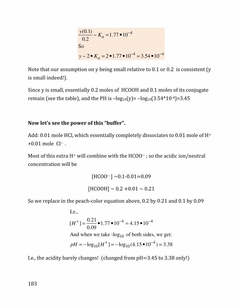
183
4
4 4
(0.1)~ 1.77 10
0.2
So
~ 2 2 1.77 10 3.54 10
a
a
yK
y K
−
− −
= •
• = • • = •
Note that our assumption on y being small relative to 0.1 or 0.2 is consistent (y
is small indeed!).
Since y is small, essentially 0.2 moles of HCOOH and 0.1 moles of its conjugate
remain (see the table), and the PH is –log10(y)= –log10(3.54*10-4)=3.45
Now let’s see the power of this “buffer”.
Add: 0.01 mole HCl, which essentially completely dissociates to 0.01 mole of H+
+0.01 mole Cld . Most of this extra H+ will combine with the HCOO− ; so the acidic ion/neutral concentration will be
îHCOO− ñ ~0.1-0.01=0.09 îHCOOHñ ~ 0.2 +0.01 ~ 0.21
So we replace in the peach-color equation above, 0.2 by 0.21 and 0.1 by 0.09 4 4
10
410 10
I.e.,
0.21[ ] 1.77 10 4.15 10
0.09
And when we take -log of both sides, we get:
log [ ] log (4.15 10 ) 3.38
H
pH H
+ − −
+ −
= • • = •
= − = − • =
I.e., the acidity barely changes! *changed from pH=3.45 to 3.38 only!&

184
10.iv) Final acids/bases subpart: TITRATIONS
The goal in titrations is: find the unknown concentration of an acid or base
(called “analyte”) in a solution with a known volume.
The idea is simple: add the opposite (i.e., base to acid or vice versa); what we
add is called a “titrant”.
Titrations involve the addition of a titrant to a solution of analyte containing an
unknown amount of acid or base (i.e., the concentration of the acid is unknown).
The volume of the analyte (the acid or base in the solution) is known, but its
concentration is not known. In titration we find this unknown analyte
concentration by adding to it a known volume of a different solution (the
titrant) with a known concentration; essentially, if the analyte is acidic we add to
it a base titrant and vice versa (not exactly accurate, since a given compound can
be viewed as both acidic and basic, but it is good enough for our purposes).
The key is that there will be a concentration (the equivalence point) where
the actual amounts (moles) of the analyte and titrant will match; at that
point, the ions (H+ and OH-) from the analyte and titrant will almost
exactly match, so the pH of the solution will change to be close to neutral.
The pH change will signify that the amount of moles of the titrant added
will be the same (or close to ) the amount of initial analyte.
The amounts of H+ initially present (or added) is often called "acid equivalent";
a base equivalent is the amount of OH- in moles for a basic solution.
This stoichiometric point, to be discussed later in this section, is the point at
which the number of moles of titrant added is equal to the # of moles of analyte
in the solution, i.e., the acid and base equivalents will match (for polyprotic acids
see below);
Strong Acid-Strong Base Titrations
Mixing acids with bases, or bases with acids, the ions react thusly:
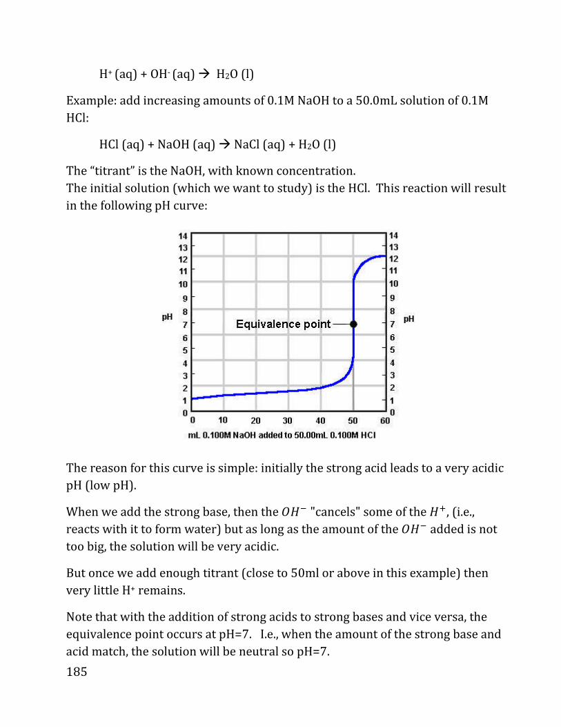
185
H+ (aq) + OH- (aq) � H2O (l)
Example: add increasing amounts of 0.1M NaOH to a 50.0mL solution of 0.1M
HCl:
HCl (aq) + NaOH (aq) � NaCl (aq) + H2O (l)
The “titrant” is the NaOH, with known concentration.
The initial solution (which we want to study) is the HCl. This reaction will result
in the following pH curve:
The reason for this curve is simple: initially the strong acid leads to a very acidic
pH (low pH).
When we add the strong base, then the ¹¨» "cancels" some of the ¨ç, (i.e.,
reacts with it to form water) but as long as the amount of the ¹¨» added is not
too big, the solution will be very acidic.
But once we add enough titrant (close to 50ml or above in this example) then
very little H+ remains.
Note that with the addition of strong acids to strong bases and vice versa, the
equivalence point occurs at pH=7. I.e., when the amount of the strong base and
acid match, the solution will be neutral so pH=7.
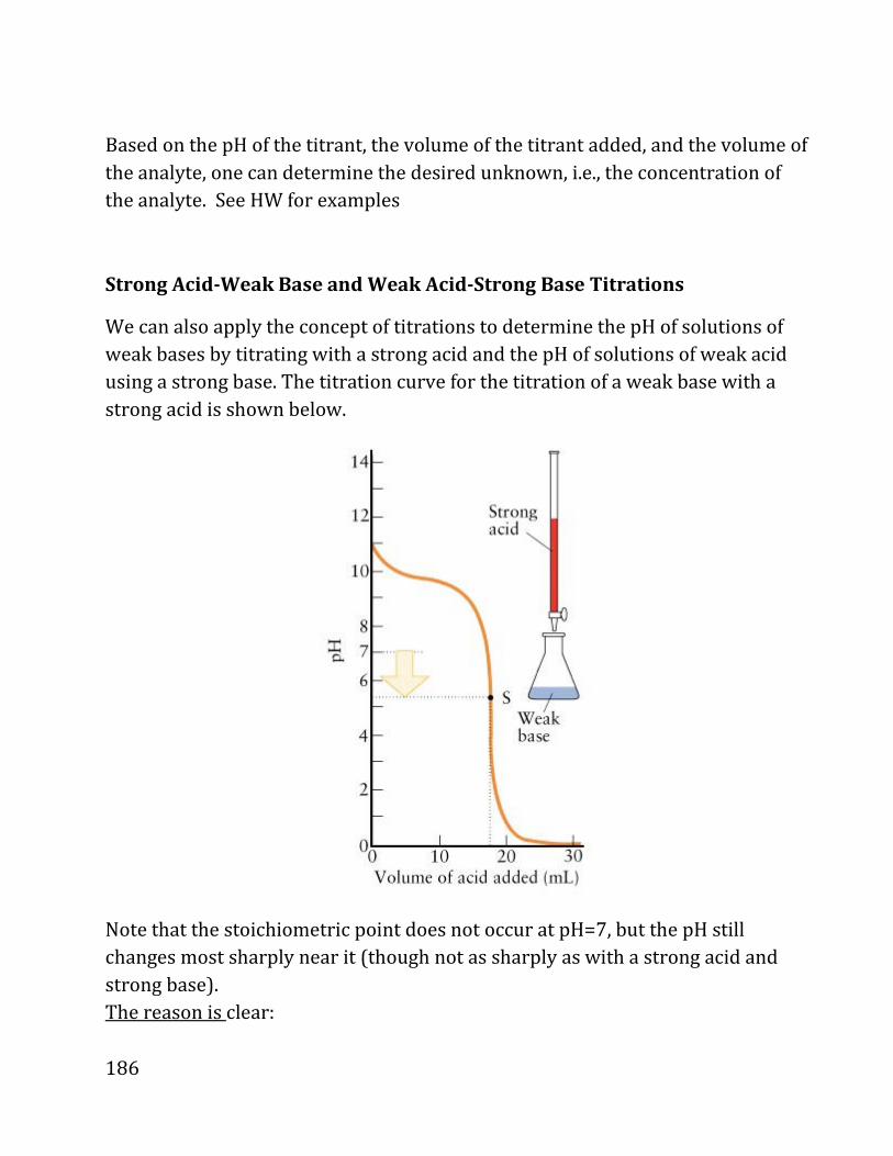
186
Based on the pH of the titrant, the volume of the titrant added, and the volume of
the analyte, one can determine the desired unknown, i.e., the concentration of
the analyte. See HW for examples
Strong Acid-Weak Base and Weak Acid-Strong Base Titrations
We can also apply the concept of titrations to determine the pH of solutions of
weak bases by titrating with a strong acid and the pH of solutions of weak acid
using a strong base. The titration curve for the titration of a weak base with a
strong acid is shown below.
Note that the stoichiometric point does not occur at pH=7, but the pH still
changes most sharply near it (though not as sharply as with a strong acid and
strong base).
The reason is clear:
187
When we throw in, say, 0.05 moles of a strong base HA to an analyte contains
0.05 moles of a weak base HA, then first, before the ions combine, essentially all
the strong acid will be ionized, i.e., we will produce initially 0.05 moles of H+;
But NOT all the weak base will dissociate, so we will have less than 0.05 moles of ¹¨» say only 0.04999 moles of the weak base dissociated.
The resulting 0.04999 moles OH- and 0.050 moles of H+ will combine and as a
result we will have a non-zero amount (0.00001 moles) of H+ and a much
smaller amount of OH- (determined from Kw/(concentration of H+)).
So therefore, at the equilibrium point for a strong base and a weak acid, where
the same number of moles of acids and basis were thrown in, the solution will
have a non-neutral pH (in our case 10-5 moles).
We won’t review the opposite (strong base with weak acid), but it is obviously
analogous.
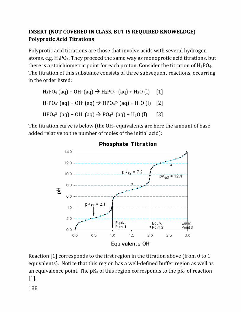
188
INSERT (NOT COVERED IN CLASS, BUT IS REQUIRED KNOWELDGE)
Polyprotic Acid Titrations
Polyprotic acid titrations are those that involve acids with several hydrogen
atoms, e.g. H3PO4. They proceed the same way as monoprotic acid titrations, but
there is a stoichiometric point for each proton. Consider the titration of H3PO4.
The titration of this substance consists of three subsequent reactions, occurring
in the order listed:
H3PO4 (aq) + OH- (aq) � H2PO4- (aq) + H2O (l) [1]
H2PO4- (aq) + OH- (aq) � HPO4
2- (aq) + H2O (l) [2]
HPO42- (aq) + OH- (aq) � PO4
3- (aq) + H2O (l) [3]
The titration curve is below (the OH- equivalents are here the amount of base
added relative to the number of moles of the initial acid):
Reaction [1] corresponds to the first region in the titration above (from 0 to 1
equivalents). Notice that this region has a well-defined buffer region as well as
an equivalence point. The pKa of this region corresponds to the pKa of reaction
[1].
189
When we add enough base (more than the amount of acid originally present)
then the polyprotic acid will turn from neutral to the first ionic form (in this
case, H2PO4d ); that's the region beyond Equiv. point 1.
When we add even more base (beyond twice the initial amount of acid present,
i.e., Equiv. point 2), then the polyprotic acid will shed an additional hydrogen';
Also, note that reactions [2] and [3] also have buffer regions and equivalence
points. The equivalence point of reaction [3] is less well defined because the pKa
is so close to that of water.
END OF INSERT
190
PRECIPITATION
(i) Solid/pure liqu. Reactants: possibility of consuming all reactants
So far we only discussed acid/base reactions where reactants (at least some) are
dissolved.
These are equivalents of reactions with gases where there are gases on both
side.
Now we’ll tackle cases where the reactants are all solid (liquid too if the liquid is
not part of the aqueous solution, but that’s a rarity).
Example: Calcium hydroxide, a base.
Ca*OH&�*N& → Ca�ç + 2*OH»&
� . îCa�çñîOH»ñ� (if there’s equilibrium with Ca*OH&�*N& existing!)
Note that we did not divide by 1M=1 mol/L, for simplicity; and, more
importantly the concentration of the solid does not appear in the equation
for K (since the Gibbs free energy does not depend on concentration for the
solid). So unlike the previous discussions in this section, where the equality
means equality, here, it just means IF THERE’S EQUILIBRIUM BETWEEN
REACTANTS and products, such that the REACTANTNS EXIST AT
EQUILBRIUM the LHS and RHS will equal
Turns out that at room temperature, for this reaction,
�/à . 5.5 ∗ 10»H
(practice question: what’s Δ�5 then?)
Now, take a specific case – throw in 0.01M amount of [Ca*OH&�ñ – e.g., throw in
10 moles to 1000 liter, etc.

191
Even if all the reactants are consumed, i.e., from 0.01 Moles CaOH2 we make
0.01M ¬8�ç, 0.02M ¹¨»
(Two hydroxide ions for each calcium ion), then still the RHS of the highlighted
eq. will be
îCa�çñîOH»ñ� = 0.01 ∗ *0.02&� = 4 ∗ 10»H < �/à! So since the density product is lower than K, we won’t have an equilibrium
where reactants coexist – so all the Ca(OH)2 will be consumed.
In our earlier language, we’ll say that the Gm for the product side is lowered than
the Gm for the reactant side (solid calcium hydroxide), so Ca(OH)2 will be
consumed; but since this reactant is not in solution, as we consume the reactant
its Gm will not change.
Contrast this with HCl � H+ + Cl-, for example – as we consume HCl its
concentration changes so its (the HCl’s) Gm chances (is lowered), so eventually
we’ll reach equilibrium (Δ� . 0& where all reactants and products coexist.
(ii) Precipitating the solid compounds
If we increase the concentration of one of the products (in our case say OH-by
changing pH), then eventually the density product (îCa�çñîOH»ñ� ) can reach
KCa. Let’s calculate the threshold concentration of OH- required in this case to
make the first little piece of solid.
î¬8�çñ»ñ� . �/à → »ñ . � �/àî¬8�çñ . �5.5 ∗ 10»H0.01 = 0.023
Note several things:
• This threshold conc. is HIGHER than 0.02, the conc. of OH- obtained when
all the 0.01 M Ca(OH2) is released to the solution – so without another
192
source of hydroxide (another base) the calcium will not precipitate and
remain wholly in the ionic form.
• I used 0.01 for the concentration of Ca2+ in the eq. above The reason is
that we consider the case that almost all the calcium hydroxide is
dissolved, and ask what will be the concentration where just a tiny bit is
calcium is precipitated , so the ionic liquid form will still have almost the
same concentration as if none precipitated. Of course, if the conc. of OH-
was raised even further, then the conc. of the calcium ion will decrease,
and more solid calcium hydroxide will precipitate.
• We are treating things like precipitation as if they will immediately occur
when they are thermodynamically favored. In reality we can have
supersaturated solutions – we’ll discuss these later
Let’s relate the threshold conc. of OH- for precipitation to pH:
»ñ . 0.023 → ]¹¨ = − log�5 0.023 = 1.64 →
]¨ . �_ d ]¹¨ . 14 d 1.64 = 12.36
So for pH above 12.36 the calcium hydroxide will precipitate. (Just like
Lechatelier’s principle says, think about it!)
(iii) Selective precipitation.
We throw in 0.05 Mole of Mg(OH)2, which is less soluble
T[*¹¨&� → T[�ç + 2¹¨»
Kf� = 1.1 ∗ 10»��, i.e., if there’s equilibrium (i.e., if there’s solid Mg(OH)2) then
1.1 ∗ 10»�� = �f� = îT[�çñ»ñ�
Repeating the steps in the Ca(OH)2 example, we see that selective precipitation will occur when
193
»ñ . � �f�îT[�çñ . �1.1 ∗ 10»��0.05 = 1.5 ∗ 10»Ê
So
pOH = log�5*1.5 ∗ 10»Ê& = 4.82 → pH = 9.18
We therefore see that selective precipitation, i.e., precipitation of Mg(OH)2 but not of Ca(OH)2 ,occurs between pH of 9.18 and 12.36.
So:
• below pH of 9.18 – both metal ions (T[�ç, ¬8�ç& are in the solution;
• between 9.18 and 12.36, T[�ç precipitatres, i.e., is in equilibrium with the
solid Mg(OH)2; as pOH is raised from 9.18 gradually, the concentration of
the T[�ç is decreased. For example, just before the point where the
Calcium hydroxide starts precipitating, at pH-12.36, the concentration of
the Mg2+ ion will be tiny:
îMg�çñ . K� îOH»ñ� = 1.1 ∗ 10»��*0.023&� *8R]¨ . 12.36, _ℎP9P»ñ . 0.023&
îMg�çñ = 2.08 ∗ 10»¤M = 21nM
• for pH>12.36, even the calcium will precipitate.
,

194
Part 11: Electrochemistry
Overview:
11.i Oxidation-Reduction (redox) reactions: Reactions that involve the
exchange of electrons between atoms, compounds, and molecules.
11.ii Half reactions.
Appendix (required) Balancing half-reactions
11.iii Galvanic cells and batteries
11.iv Half-cell potentials; the Faraday equation
11.v Potentials; relation between free energies and potentials.
(11.i) Oxidation and reactions
• Oxidation: the loss of electrons in a redox reaction. (Think of H2O – the
hydrogens lose "part" of their electrons to the oxygen – so the hyrodgens
are oxidized) . Oxidizing agent: species in a redox reaction that is
reduced.
• Reduction: the gain of electrons (or reduction of charge) in a redox
reaction (so in H2O the oxygen is reduced). Reducing agent: species in a
redox reaction that is oxidized.
Oxidation and reduction always occur together, as electrons cannot be created
nor destroyed.
To monitor redox reactions, we can use the oxidation number: the effective
charge on a compound or atom.
• Oxidation results in an increase in oxidation number (i.e., making it more
positive); e.g., in Na2O the oxidation number of Na will be +1.
• Reduction results in a decrease in oxidation number. (E.g., in Na2O it will
be -2, i.e., decrease from 0).
195
(11.ii) Half Reactions
To properly describe a redox reaction, one must balance both the atoms and the
charge, i.e. the charge on both side of the equation must be equal. For example,
consider the net ionic equation for the oxidation of copper metal to copper(II)
ions by silver ions:
Cu(s) , Ag+(aq) � Cu2+(aq) , Ag(s) (CHARGE STILL UNBALANCED!)
While the atoms are balanced, notice that the left side of the equation has a
charge of +1, and the right side has a charge of +2. To balance the charges, write:
Cu(s) + 2 Ag+(aq) � Cu2+(aq) + 2 Ag(s)
To make balancing redox reactions easier, we can write half reactions: the
oxidation or reduction part alone. For the above reaction:
Cu(s) � Cu2+(aq) + 2 e-
Ag+(aq) + e- � Ag(s)
Now, balance the electrons by multiplying the reduction half reaction by 2 and
removing electrons.
Note that the half reactions are not just a mathematical trick; in batteries, as
we'll show later, they actually occur separately (one part of the battery has one
half-reaction, the other part has the other half reaction).
For more complicated reactions involving H's and O's, use the following insert.
196
INSERT: Rules to balance Redox equation: (not covered in
lecture but I'll expect you to know them for the exam!)
1. Identify the species being oxidized and the species being reduced from the
changes in their oxidation numbers. Write the skeletal (unbalanced)
equations for the oxidation and reduction half reactions.
2. Balance all elements in the half reactions except O and H.
3. Find the change in the Oxidation numbers of the species, and account for it
by adding electrons to the reactant or product side as the case may be.
4. Balance charge
• In acidic solution, balance charge by using H+
• In basic solution, balance charge by using OH-
5. Then balance the amount of hydrogens on both side of each half reaction
by using H2O
6. Multiply all species in either one or both of half reactions by factors that
result in equal numbers of electrons in the two half reactions, and then add the
two equations and include physical states.
7. Finally, simplify the appearance of the equation by cancelling species that
appear on both sides of the arrow and check to make sure the charges as well as
the numbers of atoms balance.
Example:
��Pò» +LxQ → v'xç + QPòx»
1) First break the reaction to two reactions that take place in 2 half-cells
��Pò» → v'xç
LxQ → QPòx»
2) Balance the element that undergoes the change in oxidation state on
either side of the equation: In this reaction, there is no need to do so, as
197
the number of species are already equal. But it may not be the case always,
as we saw in the Ag Cu example above.
3) Find the change in the Oxidation Number of the species, and account for it
by adding electrons to the reactant or product side as the case may be.
+7 +2 2
4− +→+ -5eMnO Mn
(each oxygen's formal charge is -2, so the initial manganese must be formally,
at +7 so that together we have +7+4*(-2)=-1, as the overall charge of the
manganese oxide is -1). Similarly:
-2 +6
LxQ → QPòx» + R÷»
4) Now comes the charge balancing step. Find the total charge on each side of
the equation and account for it using:
H+ in acidic condition and
OH- in basic condition
24 5 8 He
−− +++ →+MnO Mn
(before the 8H+ were added to the eq. above, the left hand side had charge
-6, the right +2)
And similarly: LxQ → QPòx» + 8P» + êëLç
5) Add H2O to balance the # of hydrogens on either side:
4 225 48e HMnO Mn H O
− +− ++ + +→ ¨� + 4¨�¹ → ¹��» + 8P» + 10¨ç
If you’ve done parts 1 to 5 correctly, all oxygens should balance out.

198
6) Now just multiply by factors to make the # of electrons in the two half
cells equal, add the two half-=reactions up, write the final equation…and
you’re done!
4 225 8 4e HMnO Mn H O
− +− ++ + +→ X8
¨� + 4¨�¹ → ¹��» + 8P» + 10¨ç X5
i.e.,
24 240 64 32 O8 8e HMnO HMn− +− ++ + +→
5¨� + 20¨�¹ → 5 ¹��» + 40P» + 50¨ç
So finally add them up to get (after cancelling 40e- , 50H+ , and 20H2O on
both sides) :
���Pò» + ELxQ+ êòLç → Rv'xç + EQPòx» + êxLxP
The manipulations done here are important later for the discussions of
batteries (actually, steps 1-3 are the crucial ones for batteries, the next steps are
less crucial).
END OF INSERT: RULES OT BALANCE REDOX REACTIONS

199
(11.iii) Galvanic Cells and Batteries
Electrochemical cell: device in which an electric current is either produced
by a spontaneous chemical reaction or used to bring about a
nonspontaneous reaction.
Galvanic cell: electrochemical cell in which a spontaneous chemical reaction is
used to generate an electric current
We use special type of Galvanic cells every day. For example, batteries are one
type of Galvanic cells, in which the materials are sealed within the battery in
individual cells, and the cells are linked directly so that the voltage generated in
each can be added to give a higher total voltage. Also, fuel cells are a type of
Galvanic cell, but in these, the materials that participate in the redox reaction are
constantly added and the products are taken away.
Structure of Galvanic Cells
If we simply mix two species that undergo a redox reaction, energy is released as
heat, but no electricity is generated. However, if we separate the reactants and
provide a pathway for the electrons to travel, the electrons can do work,
generating an electric current.
A galvanic cell consists of two electrodes, or metallic conductors, which make
electrical contact with the contents of the cell but not with each other, and an
electrolyte, an ionically conducting medium, inside the cell.
The two electrodes are called the:
Anode, at which oxidation takes place, and
Cathode, at which reduction takes place
Electrons are released by the oxidation half reaction at the anode, travel through
the external circuit, and reenter the cell at the cathode, where they are used in
the reduction half reaction.
Acronym: AOL – Anode: Oxidation, Loss of electrons
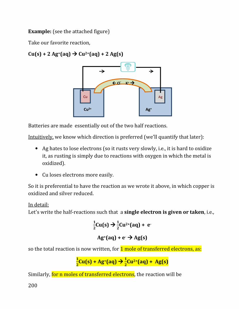
200
Example: (see the attached figure)
Take our favorite reaction,
Cu(s) + 2 Ag+(aq) ���� Cu2+(aq) + 2 Ag(s)
Batteries are made essentially out of the two half reactions.
Intuitively, we know which direction is preferred (we'll quantify that later):
• Ag hates to lose electrons (so it rusts very slowly, i.e., it is hard to oxidize
it, as rusting is simply due to reactions with oxygen in which the metal is
oxidized).
• Cu loses electrons more easily.
So it is preferential to have the reaction as we wrote it above, in which copper is
oxidized and silver reduced.
In detail:
Let's write the half-reactions such that a single electron is given or taken, i.e.,
êxCu(s) ���� êxCu2+(aq) + e-
Ag+(aq) + e- ���� Ag(s)
so the total reaction is now written, for 1 mole of transferred electrons, as:
êxCu(s) + Ag+(aq) ���� êxCu2+(aq) + Ag(s)
Similarly, for n moles of transferred electrons, the reaction will be
Cu Ag
���� Cl¯ K+ ����
Cu2+ Ag+
201
'xCu(s) + nAg+(aq) ���� 'xCu2+(aq) + nAg(s)
We'll see shortly why it is important to write it in such a form.
In the anode, the copper electrode is oxidized, so copper ions join the solution.
The electrons leave the anode and will like to reach the cathode, where they
combine with the silver-ions (Ag+) to form a solid silver, i.e., silver is deposited
on the cathode.
The salt bridge is needed, since without it there will be an accumulation of
electrons in the cathode.
But with the salt bridge, there will be charge balancing;
E.g., for a KCl salt-bridge:
• In the anode, as electrons leave the anode, and positively-charge copper is
released to the solution, negative Cl¯ ions come from the salt bridge and
balance the charge.
• And analogously for the cathode, where K+ ions come from the salt bridge
to the solution to replace Ag+ ions which are deposited on the curve.
To quantify the battery, we need to consider the next section:
202
(11.iv) Potentials; relation between free energies and potentials,
and Faraday equation
We know that the amount of useful electric work remaining is essentially related
to the free energy difference in the reaction.
So the Gibbs free energy difference for n moles of transferred electrons is
then
( ) ( ) ( ) ( )
( ) ( )( ) ( ) ( )( )
products reactants
2
2
1 1
2 2
i.e.,
1
2
tot
tot m m m m
totm m m m
G G G
G n G Cu G Ag G Cu G Ag
GG Cu G Cu G Ag G Ag
n
+ +
+ +
∆ = −
∆ = + − −
∆= − − −
Therefore:
( )21 1
2 2
tot
CATHODEANODE
GG Cu Cu e G Ag Ag e
n
+ − + −∆ = ∆ → + − ∆ → +
14442444314444244443
We did not include, for brevity, the phases; i.e., Cu and Ag are solids, and the ions
are in aqueous solutions, e.g., Cu2+(aq.).
This is a very interesting form, since it allows to break the free energy difference
in the battery, to a difference between half-cell potentials, i.e., the
difference between the free energy of reactions per electron in the cathode
and anode.
In principle, the highlighted expression is all that should have been needed for
us to determine the electric properties of the battery.
For historical reasons, however, two changes in the expression are done;
(1) we subtract a reference quantity and (2) divide by a negative constant.
203
THE REFERENCE REACTION
The reference, refG∆ , is defined customarily, at any temperature, as the G∆
(i.e., free energy difference) for a half-cell made of H+ ions in solution converting
to (or "reduced to") H2 gas:
02
1∆ eH H
2refG G + −
∆ ≡ + →
The "umlaut " (o superscript) refers to standard conditions, i.e., the proton
concentration is 1M=1m/L, and the gas is at 1 bar.
The only difference of the H+ to H2 cell and the Ag+ to Ag half-cell is that the
reduced hydrogen will be gas rather than solid as in the case of silver. Also, in
practice such a half cell will involve a catalyst, such as platinum, that will "lower
the barrier" to reaction and therefore speed it up (see later); the catalyst,
however, does not change the potential, just speeds up the reaction.
ENERGY TO VOLTAGE:
Specifically from the expression Charge*Voltage=Energy that you learn in
physics, it follows that
Voltage=Energy/Charge,
i.e., we can get a voltage from the free energy change by dividing it by F, the
charge of one mole
F=eNAvogardo~96,500 Coulomb/mol
where e is the absolute value of the charge of the electron, and to remind you – a
Columb is the amount of charge that a current of 1 Ampere carries in 1 second.
Further, we divide by minus, so a negative free energy difference, which
means that the system really likes to react, will translate to a very positive
potential.
So the cell potential (voltage) is;

204
( )0 2 21 1 1E Cu |Cu ∆ Cu e Cu ∆
2 2m refG G
F
+ + − = − + → −
Where we subtracted a constant which does not change the total battery voltage.
Specifically, defining the battery voltage as the difference between the two cells,
i.e., here as:
( ) ( )0 0 2 0E E Cu |Cu(cell) E Ag |Ag+ +≡ −
we see that the half-cell is related to the free energy difference
1.
( ) ( )
0
0 2 0
2
E
E Cu |Cu E Ag |Ag
(
1 1∆ Cu e Cu ∆
l
2
cel )
2m refG G
+ +
+ −
∆
− =
+ → −
−
=
( )∆ Ag e Ag ∆m refG G+ − → −− +( )
( )21 1∆ Cu e Cu ∆ Ag e Ag
2 2m m
tot
F
G GG
F nF
+ − + − + → + → ∆ = −
−
= −
i.e. we get the:
Faraday equation
0
0
( )
i.e.,
tot
tot
GE cell
nF
G nF E
∆∆ = −
∆ = − ∆
(Most books will not use the "tot" subscript).

205
Faraday equation and the current that passes through:
n, the number of models of electrons transferred, can be related to the total
charge transferred. Specifically: Current is : charge/time.
(Note units: Charge has units of Coulomb, current has units of
Amperes=Coulomb/sec )
Therefore,
If a current “I” is acting over time: t then: Total charge transferred= I*t
The charge is made of n moles of electrons; to get n, divide the total charge
transferred (I*t) by the charge of one mole, i.e., eNAvogadro Therefore:
n=I*t/(e Navogardo) = I*t/F
Therefore: The Faraday equation
totG nF E∆ = − ∆
can be written as:
totavogadro
FG nF E E I t
eN∆ = − ∆ = − ∆
i.e.,
totG E I t∆ = ∆
The units all work out (by construction).

206
Faraday equation and typical voltages:
The Faraday constant can be rewritten by multiplying numerator and
denominator by 1 Volt, which is defined as 1Volt=Joule/Coulomb
F=96,500 ST?UTVWVTU =96,500
XTUAST?UTVWXTUAVTU =96,500
YT?UyXTUAVTU
i.e.,
F=96.5
ZYVTUXTUA~100
ZYVTUXTUA
So batteries with potential of 1.5 Volt correspond to reactions with a difference
in the free energies (per mole of transferred electrons) of about 150 kJ/mol –
that's indeed a typical range for free energies of reactions, as we have seen
before and as the appendix in the book shows.
EXAMPLE: SMALL FLASHLIGHTS AND BATTERIES: Let's use the Faraday
relation this to estimate how much energy can be stored in a battery.
Assume a small battery, say, AA or AAA, has 0.01 moles of reactants (the reason
for adopting this number is the following guess: say each is having a molecular
weight of, very roughly, about 100 g/mol; i.e., each of the reactants weights 1g,
and for 2 reactants (one in the cathode and one in the anode) we'll have
therefore a weight of 2gram – that's typical for small batteries)
The Faraday equation, 0totG nFE∆ = − then tells us that if the battery potential is
1.5 Volt (like your typical AAA battery), then from 0.01 mol of reactants we
should be able to get
kJ/mol| | ~ 0.01mol*100 *1.5V ~1kJ ~ 1000J
VtotG nF E∆ = ∆
(We use V for volt, named after the Italian scientist Volta; don’t confuse with
volume or potential-energy).
A typical light bulb in a very small flashlight consumes ~0.5Watt, and 1Watt=
1Joule/sec, so a light bulb should be able to run on a small battery for about

207
2000secounds, i.e., about half-an-hour (till it consumes | |totG∆ =1000 Joule).
This is a surprisingly accurate estimate.
Some standard half-cell potentials:
Half reaction E0(=E0 for reduction, ( i.e.,
electron(s) addition), in volts
2
2 2
2
2
2
( ) 2 2 1.36
( ) 4 4 2 1.23
0.80
0.34
2 2 0.00 (by definition)
2 0.77
2.93
Cl g e Cl
O g H e H O
Ag e Ag
Cu e Cu
H e H
Zn e Zn
K e K
− −
+ −
+ −
+ −
+ −
+ −
+ −
+
+ +
+
+
+
+ −
+ −
�
�
�
�
�
�
�
Note:
• From these tables we get the battery potential,
e.g., for our Cu2+ + 2e- �� Cu anode and Ag++e-��Ag cathode, we get:
Δj5 . j5*Y8RZWOP& d j5*8AWOP& . 0.80 − 0.34 = 0.46V
• These umlaut (o) in these cell potentials refers to standard conditions,
i.e., all reactants and products species in solution at 1M=1mol/Liter, and
all gases at 1bar. We’ll talk later about what happens to these voltages
when the reactants get consumed as the battery is working – in short, not
much until the end of the life of the battery,
• The table follows the trend for electron affinity/ionization expected; i.e.,
O2 likes to add an electron, so the potential for reduction is high (i.e., the
free energy for the reaction where oxygen adds an electron is very

208
negative).
Conversely, K+ doesn’t like to add an electron so much, so the potential is
negative.
• By construction, the half-cell potentials for Hydrogen (i.e., proton
converting to hydrogen) are zero. (Since in the definition of the
potential, we subtract the reference Gibbs free energy, which is exactly
the free energy of proton to add H!)
• The potentials refer to the free energy per transferred electron, so they
are invariant to multiplying the reaction by an integer multiple;
i.e.,
The potential for 2 2Zn e Zn+ −+ � is the same as for 21 1
2 2Zn e Zn
+ −+ �
(in the first case we calculate the free energy for 2 2Zn e Zn+ −+ � and
divide by 2, in the second case we divide by 1)
As a corollary, the potentials for a combined reaction are averaged (rather
than summed), e.g.,
( )0 2 0 01( 2 ) ( ) ( )
2E Cu e Cu E Cu e Cu E Cu e Cu
+ − + − + + −+ = + + +� � �
i.e., in the left reaction 2 electrons are transferred, so we divide by 2.
(from tables: Left side = 0.34V
Right side= 1/2 * (0.16 V + 0.52 V )=0.34V
So both sides agree , as expected )
209
(11.v) Nernst Equation
The Nernst equation allows us to calculate the electric potential of a cell in non-
standard conditions. This is important as cells in real life are almost never in
standard conditions. The Nernst equation follows from the relation we learned
0 lnG G RT Q∆ = ∆ +
When combined with the Faraday relation (now we remove the subscript "tot",
as we know it refers to the full battery; since we don’t refer to standard
condition we drop the umlaut (o) in the Faraday equation)
G nF E∆ = − ∆
we get
lnln
o oG G RT Q G RT
E QnF nF nF nF
∆ ∆ + ∆∆ ≡ − = − = − −
i.e.,
0 lnRT
E E QnF
∆ = ∆ −
Note: RT/nF is a very small factor:
J8.3 300K
VK mol 0.026J/mol
• 96500 V
roomRT
nF nn
= =
Therefore, for a reaction with n=1, a change of Q of a factor of 2 will only change
the potential by 0.026V *ln(2) ~ 0.02 V. This is the reason that batteries are
so stable.
210
INSERT: NOT Covered IN CLASS, BUT REQUIRED: NERNST EQ. EXAMPLE
An example will show how to use the Nernst equation in practice, and will
also show in more detail how the Nernst equation predicts that batteries
will be very stable throughout their lifetime.
Take a Zn Ag battery (of course, it will be usually too expensive to make a
battery with silver, but it serves our purpose).
Write the two half-cell reaction for simplicity with n=2 transferred electrons
Zn � Zn2++2e-
(Anode, oxidation; written as reverse of reduction; E0(reduction)=-0.77)
Also
2Ag++2e-�2Ag (Cathode, E0(reduction)=0.80)
So:
�j5 . 0.80 − *−0.77& = 1.57?Further, add the half-cell reactions to get:
Zn+2Ag++2e- � Zn2++2e-+2Ag
Zn(s)+2Ag+(aq.) ���� Zn2+ (aq.)+2Ag(s)
Where we added the relevant phases. Further, since only the ions are in
aqueous solution (the neutrals are solids), then
2
2
[ ( .)]
[ ( .)]
Zn aqQ
Ag aq
+
+=
Assume that we start with
[Zn2+]start=0.01 M, [Ag+]start=0.03 M,
then, after an amount "x" of change of concentration of zinc has happened, the
concentrations are (all in mol):
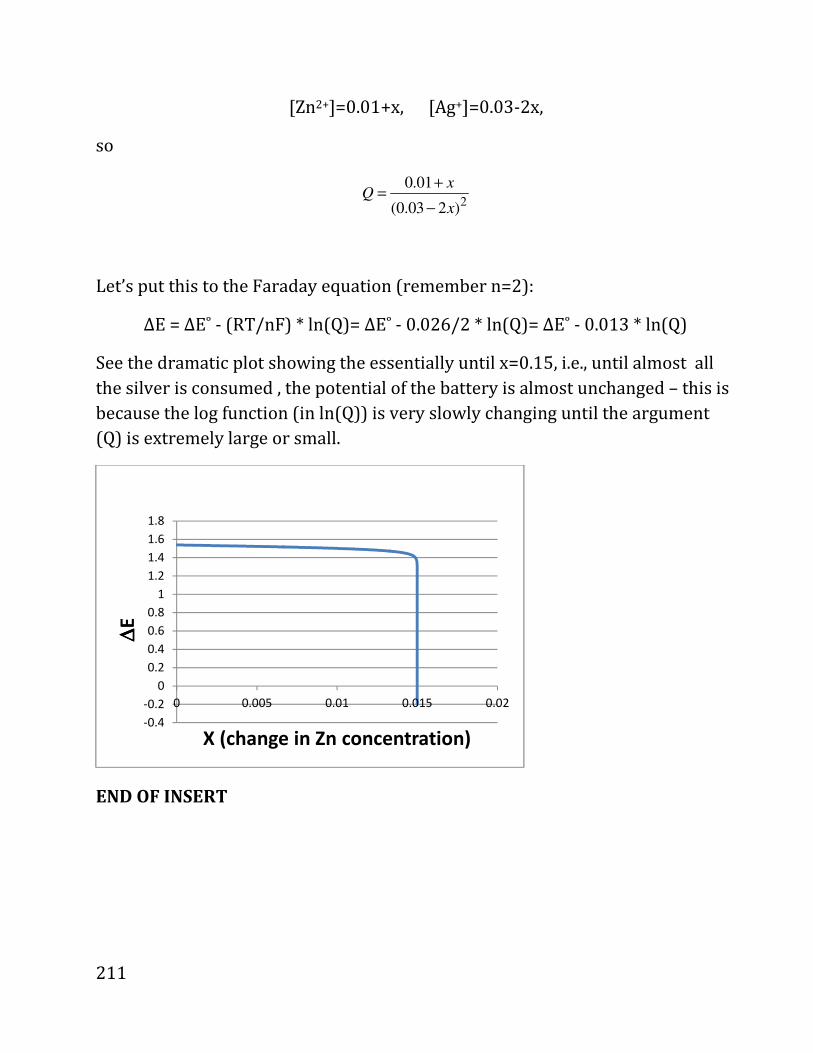
211
[Zn2+]=0.01+x, [Ag+]=0.03-2x,
so
2
0.01
(0.03 2 )
xQ
x
+=
−
Let’s put this to the Faraday equation (remember n=2):
∆E = ∆E˚ - (RT/nF) * ln(Q)= ∆E˚ - 0.026/2 * ln(Q)= ∆E˚ - 0.013 * ln(Q)
See the dramatic plot showing the essentially until x=0.15, i.e., until almost all
the silver is consumed , the potential of the battery is almost unchanged – this is
because the log function (in ln(Q)) is very slowly changing until the argument
(Q) is extremely large or small.
END OF INSERT
-0.4
-0.2
0
0.2
0.4
0.6
0.8
1
1.2
1.4
1.6
1.8
0 0.005 0.01 0.015 0.02
∆∆ ∆∆E
X (change in Zn concentration)
212
Part 12: Kinetics
Big field; here we’ll cover:
(I) Rates;
(II) Unimolecular and bimolecular elementary steps, and half-lives
(III) Including back reactions to give rates of complicated reactions
(IV) Steady state and local equi. Approximations
(V) Equilibrium
(VI) The dependence of the rate constants on T
(VII) Enzymes (if time permits).
There is a whole course (110B, highly recommended) devoted to kinetics as well
as stat. mech.; we won’t have too much time so we’ll omit many topics
(polymerization, combustion, rate-constants details, etc.)
(I) RATES:
All rxn, with time, reach equi.
Some go all the way “to the right”
H2+ ½ O2 � H2O
(At Eq., virtually no H2, O2 left.)
Some “never happen”, i.e., only reactants remain, e.g.,
NaCl(s)� Na(s)+1/2 Cl2(g)
Many are in between with both reactants and products coexisting in significant
amounts:
3 2 4( ) ( ) ( ) ( )NH aq H O s NH aq OH aq+ −+ → +
213
For this reaction, at Eq. all reactants and products exist in appreciable amounts.
REACTION RATES:
When reactions occur, e.g.,
aA+bB � xX +yY+zZ
(and we can also have that the reaction proceeds in the opposite direction,
products to reactants), then we can relate the change in the moles, i.e.,
1 [ ] 1 [ ] 1 [ ] 1 [ ] 1 [ ]d A d B d X d Y d Zrate
a dt b dt x dt y dt z dt≡ − = − = = =
For example, in 3NO � N2O+NO2, for every three moles of NO consumed, 1 mol
of N2O and 1 mol of NO2 will be made, so
2 2[ ] [ ]1 [ ]
3
d NO d N Od NOrate
dt dt dt= − = =
The question then what is this rate, (which we can write as rate=(1/x)d[X]/dt ? )
In some cases the rate is very simple (I.e., depends in a simple way on the
concentrations of the products and reactants) , in others very complicated.
There are three prevalent questions in kinetics:
1) From the rates, what happens in equilibrium;
2) How do the rate change in time (i.e., and from that how the
concentrations change in time).
3) Can we represent the rates in terms of simpler ingredients (like “Lego
blocks”)
Let’s start with the 3rd point:
A huge simplification, which is NOT ALWAYS VALID is to assume that the rate is
made from two components, a “forward” rate which depends on the reactants
concentration, and a “backward” rate which depends on the products
concentration. For the “general” reaction above this will amount to writing:
([ ],[ ]) ([ ],[ ],[ ])forward backwardrate rate A B rate X Y Z= −
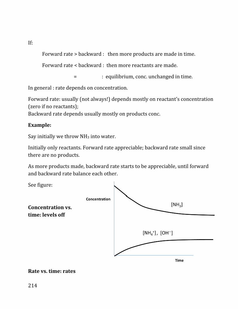
214
If:
Forward rate > backward : then more products are made in time.
Forward rate < backward : then more reactants are made.
= : equilibrium, conc. unchanged in time.
In general : rate depends on concentration.
Forward rate: usually (not always!) depends mostly on reactant’s concentration
(zero if no reactants);
Backward rate depends usually mostly on products conc.
Example:
Say initially we throw NH3 into water.
Initially only reactants. Forward rate appreciable; backward rate small since
there are no products.
As more products made, backward rate starts to be appreciable, until forward
and backward rate balance each other.
See figure:
Concentration vs.
time: levels off
Rate vs. time: rates

215
level off and match eventually.
(II) ELEMENTARY REACTIONS
Luckily in many cases we can understand complicated rates as the “result of one
or several elementary reactions.”
The 2 basic ingredients are :
• Unimolecular reactions , A� products
• Bimolecular reactions, A+B� products
We first write these reactions as if the backward rate is zero; later, we will see
how these basic ingredients (forward uni- and bi-molecular reactions) can be
used to understand reactions which go both backward and forward.
But for right now, it will be forward only; so let’s tackle each case.
Elementary Unimolecular reactions:
1kA products→

216
Examples of unimolecular decays:
• Radioactive decay – the half-lives of radioactive elements ranges
between billions of years and tiny fractions of seconds.
• Transition state – when molecules collide (typically in bimolecular
reactions, see below), the transition state (see later) usually decays by
itself.
• Excited molecules – more generally, molecules can be excited not just by
collisions but e.g., by radiation, and then the excited state decays.
Many unimolecular reactions are not really unimolecular, but are “disguised”
bimolecular, as we’ll see
Mathematically, we write:
1
[ ][ ]
d Ak A
dt= −
(Note: as mentioned above, our analysis below assumes we can ignore the back
reactions; that’s OK for radioactive decay but in many other cases we do have to
include the back reactions (products � A), as we’ll do later)
Here, k1 is a constant, which has units of 1/time (d[A]/dt has units of
concentration/time, [A] has units of concentration, so k1 has to have units of
1/time so the units match).
(Note: k has nothing to do with Boltzmann’s constant which you may
encounter in the class).
Even without doing any math we can guesstimate how long it takes for the
reaction to proceed “significantly”, i.e., for the concentration to fall by a
factor of, say, 2:
T(half-life) = Time for concentration to fall by 2 ~ 1/k1
This is because the only quantity with units of time we have in this problem is
1/k1 !
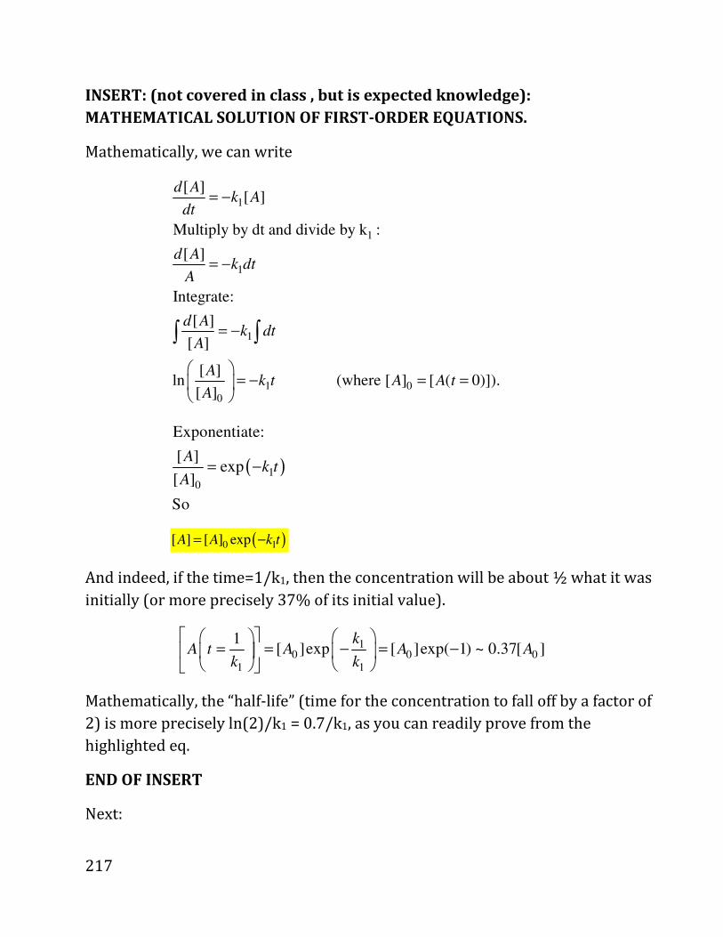
217
INSERT: (not covered in class , but is expected knowledge):
MATHEMATICAL SOLUTION OF FIRST-ORDER EQUATIONS.
Mathematically, we can write
1
1
1
1
1 00
[ ][ ]
Multiply by dt and divide by k :
[ ]
Integrate:
[ ]
[ ]
[ ]ln (where [ ] [ ( 0)]).
[ ]
d Ak A
dt
d Ak dt
A
d Ak dt
A
Ak t A A t
A
= −
= −
= −
= − = =
∫ ∫
( )10
Exponentiate:
[ ]exp
[ ]
So
Ak t
A= −
( )0 1[ ] [ ] expA A k t= −
And indeed, if the time=1/k1, then the concentration will be about ½ what it was
initially (or more precisely 37% of its initial value).
10 0 0
1 1
1[ ]exp [ ]exp( 1) ~ 0.37[ ]
kA t A A A
k k
= = − = −
Mathematically, the “half-life” (time for the concentration to fall off by a factor of
2) is more precisely ln(2)/k1 = 0.7/k1, as you can readily prove from the
highlighted eq.
END OF INSERT
Next:

218
Elementary bimolecular reactions: the most important type of elementary
reactions.
kA B AB+ →
[ ][ ][ ],
[ ] [ ][ ][ ],
d ABk A B
dt
d A d Bk A B
dt dt
=
= = −
Note units, k has units now of 1/ ( (molar-density) time) (it multiplies molar
density squared to give molar density over time, so it needs to have units of
inverse(time*molar-density).
Physically, the reason for this rate law can be understood by realizing what
happens when the concentration is, e.g., made to be 10 times higher (e.g., for
gases, reduce the volume by a factor of 10); then, in a given volume there will be
10 times as many molecules (say “A”), and each of them will have 10 times as
many chances to interact with a “B” (since the conc. of B was also increasing), so
the rate is becoming 100 times as big – and that’s what k[A][B] will indeed give.
More precisely, the reaction above is a “heterogeneous bimolecular reaction”;
we’ll deal mathematically below with: “homogenous bimolecular reaction”,
A+A�A2;
(Note stoichiometry; if we only have A, i.e., homogenous reaction,
then d[A]/dt = -2k[A]2 , i.e., d[A2]/dt = -1/2 d[A]/dt).
We’ll consider first the A+A���� A2 homogenous case
Physical considerations: If there are no back reactions we can also integrate
these reactions; before the math. note that physically we expect that as the
product dwindle with time, their decay will be much slower. To see this, let’s
look at the instantenous decay rate,
(1/[A]) d[A]/dt

219
A quantity which has the units of 1/time, so it is a measure of how fast the
reaction goes.
In unimolecular decay (1/[A]) d[A]/dt is fixed, i.e., it is k1. For bimolecular
reactions this relative decay becomes smaller in time; e.g., for the A+A�A2
reaction, as [A] is, say, ten times smaller , d[A]/dt becomes 100 times smaller, so
the relative decay becomes (1/(0.1)) * (0.1)2 = 0.1 of what it was. So: the
smaller the density the slower the decay.
A little more quantitatively, we can estimate the time it takes to reduce the
concentration significantly (say by 50%, i.e., the “half-life” time); if we start
at [A0], then the only two quantities with units will be [A0] and k, and the only
possible combination of units of time is �
[îÙ�ñ so we predict that the half-life
will now be proportional to the density squared.).
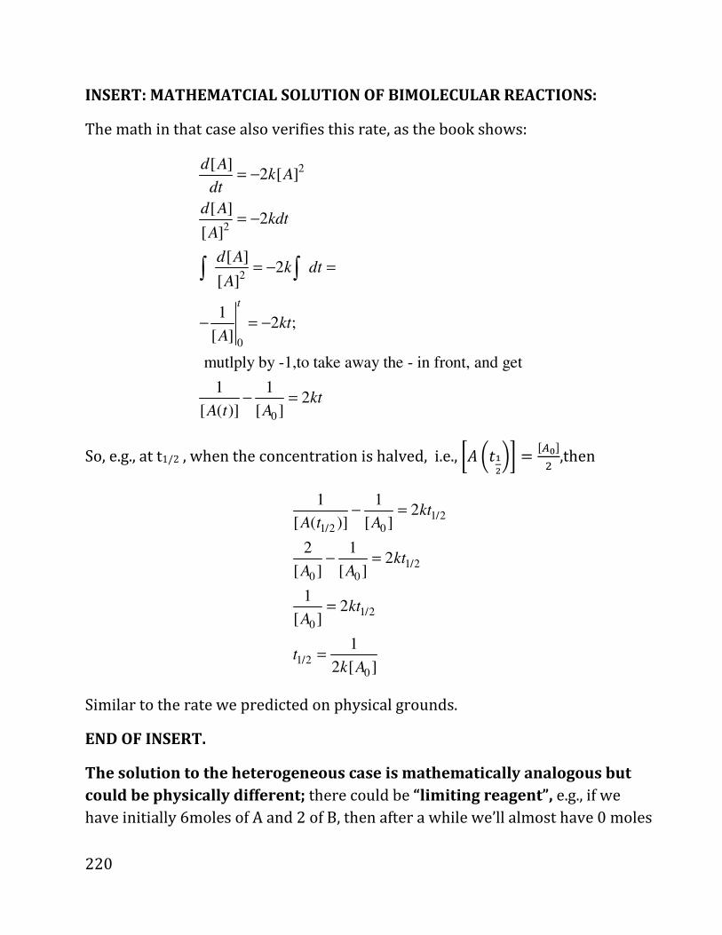
220
INSERT: MATHEMATCIAL SOLUTION OF BIMOLECULAR REACTIONS:
The math in that case also verifies this rate, as the book shows:
2
2
2
0
0
[ ]2 [ ]
[ ]2
[ ]
[ ]2
[ ]
12 ;
[ ]
mutlply by -1,to take away the - in front, and get
1 12
[ ( )] [ ]
t
d Ak A
dt
d Akdt
A
d Ak dt
A
ktA
ktA t A
= −
= −
= − =
− = −
− =
∫ ∫
So, e.g., at t1/2 , when the concentration is halved, i.e., \ã �R�©�] . îÙ�ñ� ,then
1/21/2 0
1/20 0
1/20
1/20
1 12
[ ( )] [ ]
2 12
[ ] [ ]
12
[ ]
1
2 [ ]
ktA t A
ktA A
ktA
tk A
− =
− =
=
=
Similar to the rate we predicted on physical grounds.
END OF INSERT.
The solution to the heterogeneous case is mathematically analogous but
could be physically different; there could be “limiting reagent”, e.g., if we
have initially 6moles of A and 2 of B, then after a while we’ll almost have 0 moles
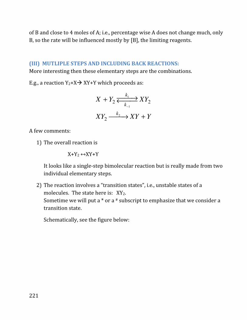
221
of B and close to 4 moles of A; i.e., percentage wise A does not change much, only
B, so the rate will be influenced mostly by [B], the limiting reagents.
(III) MUTLIPLE STEPS AND INCLUDING BACK REACTIONS:
More interesting then these elementary steps are the combinations.
E.g., a reaction Y2+X� XY+Y which proceeds as:
1
1
2
2 2
2
k
k
k
X Y XY
XY XY Y
−
→+ ←
→ +
A few comments:
1) The overall reaction is
X+Y2 ↔XY+Y
It looks like a single-step bimolecular reaction but is really made from two
individual elementary steps.
2) The reaction involves a “transition states”, i.e., unstable states of a
molecules. The state here is: XY2.
Sometime we will put a * or a # subscript to emphasize that we consider a
transition state.
Schematically, see the figure below:

222
XY2 is a transition state, i.e., a state of the molecules which lives for a short time.
3) Let’s write the math; for each compound we need to consider all the
reactions (with correct signs) that make or destroy it
1
1
2
2 2
2
k
k
k
X Y XY
XY XY Y
−
→+ ←
→ +
d[X]/dt = -k1 [X][Y2] + k-1[XY2]
d[Y2]/dt = -k1 [X][Y2] + k-1[XY2]
d[XY2]/dt = k1 [X][Y2] - k-1[XY2]-k2[XY2]
d[XY]/dt = k2[XY2]
d[Y]/dt = k2[XY2]
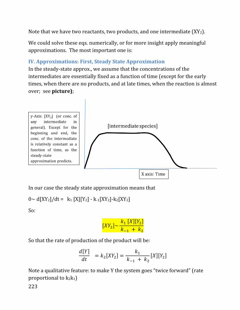
223
Note that we have two reactants, two products, and one intermediate (XY2).
We could solve these eqs. numerically, or for more insight apply meaningful
approximations. The most important one is:
IV. Approximations: First, Steady State Approximation
In the steady-state approx., we assume that the concentrations of the
intermediates are essentially fixed as a function of time (except for the early
times, when there are no products, and at late times, when the reaction is almost
over; see picture);
In our case the steady state approximation means that
0~ d[XY2]/dt = k1 [X][Y2] - k-1[XY2]-k2[XY2]
So:
îÐ0�ñ~ ��îÐñî0�ñ�»� + ��
So that the rate of production of the product will be:
Oî0ñOR . ��îÐ0�ñ . ���»� + �� îÐñî0�ñ Note a qualitative feature: to make Y the system goes “twice forward” (rate
proportional to k2k1)

224
(V) EQUILIBRIUM
The stage step in a reaction is when it is over (or approaching completion). The
result is boring if it is only a forward reaction, i.e., no reactants remain, only
products (though it could be quite interesting if we have several option for
different products, and the details of the react. determine which of the possible
products is made). However, in many cases there will be some reactants and
some products rmeaining, so then we’ll like to use the rates to tell us the
concentrations
Before considering the equilibrium let’s do one change – allow products to back-
react, otherwise in equilibrium we’ll only have products. I.e., we’ll modify the
reaction to be:
1
1
2
2
2 2
2
(I)
(II)
k
k
k
k
X Y XY
XY XY Y
−
−
→+ ←
→ +←
With a rate constant “k-2” to go back from the products XY+Y to the transition
state.
Let’s only concentrate on reaction I, reactants to transition state.
Now at equilibrium the amount of reactants does not change
0 . *8RPåXQ. & OîÐñOR . d��îÐñî0�ñ +�»�îÐ0�ñSo the concentration of the transition state is
î^_xñ . `ê`»ê î^ñî_xñ
So we can use a thermodynamic relation like we had before
î^_xñî^ñî_xñ . +a
225
Where we defined an “equilibrium constant”,
+a . `ê`»ê
Let’s define a “”Free energy of the transition state”,
�∗ ≡ �U*Ð0�&
which will be calculated by imposing the K vs. G relation that we derived earlier
+a~yz{ �d%∗ d %ö÷bc=b'=ùtu �
Put differently G* will be defined so as to fulfill this relation above, i.e., I is
defined as
�∗ . �ÄÇà�ÒàÛÒÈ + ED^A*�d&
Also, ���������� . �U*Ð& + �U*0�&,
(One word of caution: the reason for having a ~ sign is that we ignore terms like
RT/P which are necessary when we go from K to Kc, as we learned earlier. For
this reason we are “missing units”, i.e., K as we defined it has units of 1/density,
so it cannot be an exponent unless we divide by another quantity with the same
units; but for our qualitative discussion this is OK).
And we can summarize this as:
`ê`»ê .
î^_xñî^ñî_xñ . yz{ �d *%∗ d %ö÷bc=b'=ù&tu �
So the lesson is that there is a relation (the yellow-highlighted eqs. above)
between the forward and backward rate constant; they are related by the
exponential of the free energy difference between the transition state and
the initial state.
This shows you that if the transition state free energy is much larger than RT,
than the forward rate, k1, has to be very small (as “K” will be very small). I.e., to
get a high occupation of the transition state, which will allow you to have fast

226
reaction, you need to lower the free energy of the transition state, which will
make k1 higher.
Now let’s briefly consider the second reaction, i.e.,. transition state to products.
Using exactly the same mathematics, we will get
`»x`x . î^_xñî^_ñî_ñ . yz{|d*%∗ d %eö)ýbc=ù&tu }
(Note that now k2 is at the denominator, since it refers to reacting away from
the transition state, just like k-1 ).
Let’s divide the last two highlighted equations, so we get:
`»x`»ê`x`ê . î^_ñî_ñî^ñî_xñ . yz{|d *%eö)ýbc=ù d %ö÷bc=b'=ù&tu }
Note that we get the mass-reaction law – i.e., the densities are related by a
constant.
îÐ0ñî0ñîÐñî0�ñ . ��
where
�� . �����»��»� Note that this is the mass reaction law, derived from rate kinetics!
227
(VI) The dependence of the rate constants on T
We can understand how the rate constant depends on T qualitatively (for
elementary reactions). Let’s consider a typical bimolecular elementary reaction
case where the transition state could be quite high (e.g., our X+Y2� XY2 � XY+Y
reaction diagrammed above); t
Ten, let’s say that a pair of molecules (X and Y2) needs to have relative kinetic
energy above , Δ�∗ to react (where, at least approximately, Δ�∗ . �∗ d�ÄÇà�ÒàÛÒÈ, i.e., the difference in free energy between the transition state and the
reactants).
Δ�∗ is the activation free-energy (it is similar to E in the book)
Then, from the |Boltzmann distribution we know that at least approximately, the
fraction of molecules with molar energy above Δ�∗ (i.e., those molecules that
can react) is
(Fraction with E higher than E ) ~ exp(-Δ�∗/(R T))
And therefore we expect that the forward rate will be proportional to
k1 ~ exp(-Δ�∗/(RT))
Note that the rate will then be very small at low T (as we saw in the earlier
section);
So then �»� ~ constant (any molecule in the transition state breaks easily), and
k�k»� ~exp �−ΔG∗ED�
Note that this is the same as the expression we derived in the previous section,
k�k»�~ exp �−�∗ − �ÄÇà�ÒàÛÒÈED �
Arrhenius plot
Further, if Δ�∗ is made from two components, an energy term and an entropy
term,
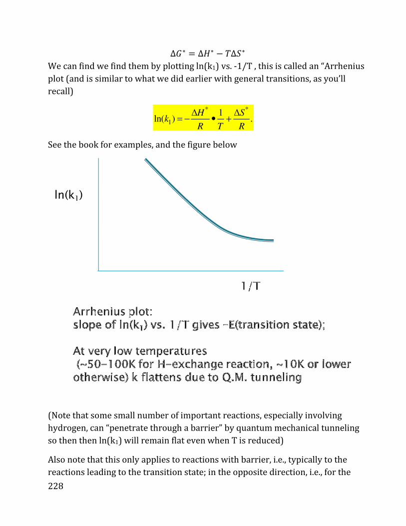
228
Δ�∗ . Δ¨∗ d DΔ ∗
We can find we find them by plotting ln(k1) vs. -1/T , this is called an “Arrhenius
plot (and is similar to what we did earlier with general transitions, as you’ll
recall)
* *
1
1) .
∆(
∆ln
H S
Rk
T R+•= −
See the book for examples, and the figure below
(Note that some small number of important reactions, especially involving
hydrogen, can “penetrate through a barrier” by quantum mechanical tunneling
so then then ln(k1) will remain flat even when T is reduced)
Also note that this only applies to reactions with barrier, i.e., typically to the
reactions leading to the transition state; in the opposite direction, i.e., for the
229
breakup from the transition state, the temperature dependence (of k-1 or k2 in
our example) will be very weak, since all molecules in the transition state will
break without barrier

230
(VII) ENZYMES:
Final kinetics topic. Important in biochem.!
Covered clearly in Oxtoby, so just a summary: the enzyme is a catalyst, enabling
the reaction (other kinds of catalysts, typically metal surfaces, are also covered).
The reactions are
1
1
2
( ) (bound enzyme, transition state)( )
( )
k
k
k
subtrateenzyme
product
E S ES
ES E P
−
→+ ←
→ +
Note that the total enzyme (defined as [E0]) is conserved, i.e., it could be either
unbound E or bound ES, i.e.,
0[ ] [ ][ ] [ ]E E S ES= + ).
The product formation rate is
2
1 2 1
[ ][ ]
using the steady state approximation, which says that the
formation of the ES transition state intermeidiary
is essentially balanced by its consumption, we get
[ ]0 ~ = [ ][ ] ( )
d Pk ES
dt
d ESk E S k k
dt−
=
− + ( )1 0 2 1
0
[ ] [ ] [ ] [ ] ( )[ ]
(where we used [ ] [ ][ ] [ ] )so
ES k E ES S k k ES
E E S ES
−= − − +
= +
1 0
1 2 1
[ ][ ][ ] ~ , i.e.,
[ ]
k E SES
k S k k−+ +
2 1 02
1 2 1
[ ][ ][ ][ ]
[ ]
k k E Sd Pk ES
dt k S k k−
= =+ +
Note that for small enzyme substrate concentration([S]) the enzyme will be
mostly free, and then the rate of production of products will be proportional to
231
the concentration of the substrate (i.e., the denominator in the expression above
will be k2+k-1, i.e., constant);
But if there is a lot of enzyme, so that the denominator will be dominated by the
substrate form (k1[S]>>k2+k-1) then
d[P]/dt ~ k2 [E0],
i.e., at high substrate concentration the reaction will look zeroth order in the
substrate density – this makes sense since then the reaction will be limited by
the amount of enzyme, not substrate.

232
Part 13. Raul's Law and Colligative properties (if
time permits!)
Physical properties of solution diff. from pure solvent:
Diff. boiling point (b.p.), vapor pressure, melting point (m.p.)
Most importantly: solutions exhibit a range of temperatures where, at the same
pressure, there’s equilibrium between liquids and vapors! This is the basis for
distillation, i.e., purifying solutions making them richer in one compound or
another, as we’ll see.
Start: Vapor pressure
Add: two liquid compounds, "1" and "2" (I label them “A” and “B” or “1” and “2”,
interchangeably) to form a solution;
Seal this solution in a fixed volume container so there will be equilibrium
between the compounds in their liquid and vapor phases
How is vapor pressure (v.p., denoted as PA , PB ) of compounds affected?
Let's concentrate on species "A", for example.
Think of: mole fraction xA (L) of A(in Liquid!).
We know what happens at the extremes

233
xA(L)=1 � pure "1" � 4Ù . 4Ù∗ where * denotes pure solvent
xA(L)=0 � no "1" � PA=0.
That’s always true. What’s in between?
If "A" and "B" are “PHYSICALLY SIMILAR liquids that interact in similar ways,
will be called “ideal mixture”, then
For ideal mixtures, Raul’s law obeyed:
Pf = xf*L)Pf∗*T&
Physically, reason that in Raul’s law vapor pressure relates to the molar
fraction in the liquid is due to equilibrium;
I.e., Raul’s law Pf = xf*L)Pf∗*T&, is really the same (up to an overall function
multiplying both sides) the same as:
98RP*�8]W9 → ^QåXQO& = 98RP*^QåXQO → �8]W9& Left: Pressure term, particles coming from vapor to liquid come at a rate which
is determined by the pressure (higher pressure � more vapor particles impinge
on the liquid);
Right: represents tendency of “A” particles to leave liquid and go to vapor. This
tendency is reduced when there is a solution, as there is more disorder (each A
now can be surrounded by only As, or B and several A’s, or 2B & several As, etc.).
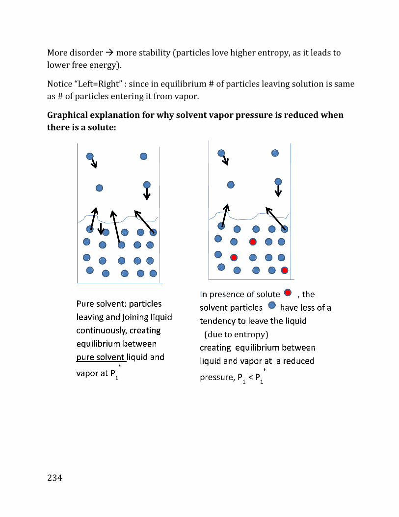
234
More disorder � more stability (particles love higher entropy, as it leads to
lower free energy).
Notice “Left=Right” : since in equilibrium # of particles leaving solution is same
as # of particles entering it from vapor.
Graphical explanation for why solvent vapor pressure is reduced when
there is a solute:
(due to entropy)

235
In solutions, vapor's composition will be different than Liquid:
Let's see this for ideal solutions, where we can work the numbers. If the solution
is ideal, we have Raul’s law
Pf = xf*L)Pf∗*T&
Pg = xg*L)Pg∗*T& E.g., “A”=toluene (methyl-benzene) , “B”=benzene, T=300K:
Pf∗*T . 300K) = 29mbar
Pg∗*T . 300K& . 99mbar
Note that toluene is less volatile than benzene (slightly bigger molecule, vdW
interactions more effective, holding the liquid slightly more together,
everything else the same).
Graphically:
xB
xA
236
Example:
Solution of toluene and benzene, 60% of liquid is “A” (toluene); the solution is in
a container and there’s equilibrium between vapor and liquid.
Question.
(i) What’s the vapor pressures of “A” and “B”
(ii) What’s the mole fraction of “A” and “B” in vapor.
Answer:
. (i) PA = xA(L) PA* = 0.60*29mbar = 17.4 mbar
PB = xB(L) PB* = 0.40*99mbar = 39.6 mbar
(ii) ÛÜÛÝÞÝ . �Ü�ÝÞÝ . �I.�,h.Hç�I.� = 30% = 0.30
Note that solution is 60% toluene, but vapor only 30% toluene!
Reason – toluene is much less volatile.:
We can use the difference in composition of vapor and liquid for:
Distillation:
Scrape the vapor; richer in one compound (above, vapor richer in Benzene).
Then repeat: Cool down vapor till it liquefies, scrape vapor; that vapor is even
richer in benzene, and continue for a few more steps.
237
Colligative properties
Next, specialize to non-volatile solutes (e.g., salt in water, or sugar in
water).
The reduction of vapor pressure for a solvent upon inclusion of a non-volatile
solute, leads to: colligative properties i.e., properties that depend on # of
dissolved solute, not on identity of such species.
First:
Vapor pressure lowering:
• Boiling temp. elevation (e.g., salty water boils at > 1000C)
• Freezing point depression:
(Salty water freeze at temp. as low as -18 0C [ 0 Fahrenheit], depending on
conc. )
• Osmotic pressure (see later).
Important prelude on Raul's law: it is always valid for solvents.
I.e., we said that Raul’s law is only valid for "ideal" mixtures; but for solvent-
solute mixtures, i.e., if one compound is much more abundant than the other,
Raul's law is valid for the solvent when any solute is inserted, as long as the
concentration of the solute is small;
So in general:P£¡¢ØÀà. x£¡¢ØÀÃÂ*L&P£¡¢ØÀÃÂ∗ *T&
Physically: the solvent molecules “like” to remain liquid a little more due to
the presence of the solute – the solvent molecules therefore will have lower
vapor pressure
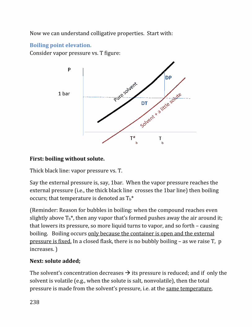
238
Now we can understand colligative properties. Start with:
Boiling point elevation.
Consider vapor pressure vs. T figure:
First: boiling without solute.
Thick black line: vapor pressure vs. T.
Say the external pressure is, say, 1bar. When the vapor pressure reaches the
external pressure (i.e., the thick black line crosses the 1bar line) then boiling
occurs; that temperature is denoted as Tb*
(Reminder: Reason for bubbles in boiling: when the compound reaches even
slightly above Tb*, then any vapor that’s formed pushes away the air around it;
that lowers its pressure, so more liquid turns to vapor, and so forth – causing
boiling. Boiling occurs only because the container is open and the external
pressure is fixed. In a closed flask, there is no bubbly boiling – as we raise T, p
increases. )
Next: solute added;
The solvent’s concentration decreases � its pressure is reduced; and if only the
solvent is volatile (e.g., when the solute is salt, nonvolatile), then the total
pressure is made from the solvent’s pressure, i.e. at the same temperature,
239
equilibrium between the mixture as liquid and as vapor will happen at lower P
once the non-volatile solute is added. (See picture).
Analogously, from the picture, we will need a higher T to reach equilibrium with
vapor at the same pressure.
Finally, without doing the math, you see from the picture that if the original
curve of P vs. T for pure solvent is “flatter” , then we will need a larger
temperature to affect the boiling – i.e., the boiling point elevation will happen at
higher T.
Mathematically: we write ODÚ . �ÚÐÈÅâ�ÒÇ
Where KB (not Kelvin, and not related to the other K’s we used!) is the boiling-
point increase parameter, which depends on solvent and the temperature.
Technical points
1): we used X£¡¢ÕÂÀ. Note that if we have salts, e.g.,
NaCl → Naç + Cl»
Then, 1mol of salt in water solution gives 2mol solutes (Naç, Cl»)
Example, 1mol of salt in 1800g of water gives
X£¡¢ÕÂÀ . n£¡¢ÕÂÀn¡ . 2mol100mol + 2mol ~0.02, where the 100 mol comes from the water, 1 mol comes from Na+, and 1mol from
Cl-; so the total # of moles is 102mol, and of which 2mol is solution. So the
answer is about 2%, not 1%, since the salt gives 2 contributions – one from
positive ions, one from the negative ones.

240
2) It is important to note that in practice when we use this equation we need to
measure the concentration in molality, as Kb is usually given in units of
K/molality. (i.e., �������jÞ;kÝl
mnjÞ;ol9Ý]
I would have preferred the concentration, but for experimentalists it is more
convenient, at least historically, to use Molality.
The experimental number for water is Kb ~ 0.5 ¦¦ �¡¢ . It is possible to estimate
this number theoretically.
Now we can turn to a completely similar phenomena:
Freezing point depression
Similar; since liquid solvent is made “more stable” by presence of solute, then
freezing temperature is lowered. For example, if we add salt to water, then,
whereas it would have frozen at 0 Celsius before, now it will freeze at a lower
temperature, as low as -18 Celsius if we add salt (and even lower for some forms
of “antifreeze”).
Formally, if the amount of solute is not too much, we write the same equation as
before
OD< .d�<ÐÈÅâ�ÒÇ
Where, as mentioned, Xsolute now stands for the Molality and not the mole
fraction.
Also, the negative sign is since the freezing point depresses (liquid is more stable
than solid);
For water :
�Æ = 0.5 K Kg /mol �< = 1.8 K · Kg/mol Physically, Kf is larger since solids & liquids are quite similar (strongly
interacting molecules) and differ only in whether the molecules are ordered.

241
Therefore, the increased stability of the liquid in the presence of the solute can
cause a big effect on freezing.
In contrast, for gas-liquid (boiling) transition, the difference between liquid and
gas is quite large, so the extra stability of the solvent is not going to affect the
transition temperature strongly.
The last colligative effect is:
Osmotic Pressure
Take a semi-permeable membrane that just lets water pass through, but not a
solute.
Use it to separate water into two compartments – e.g., in the left one put solute,
and in the right one pure water (labeled “l” for “liquid” in the figure).
Then the liquid which contains ions is more stable � water will move into the
left region, as solvent prefers region with higher stability, i.e., with more solute ‘
the extra water in the left compartment will create a higher pressure (so the
water column will rise on the left).
Analogously, in biological cells: the cells have ions, and cell wall which is
permeable to water; within the cell there will be higher P as water moves into

242
the cell. Can be as high as 50bar (as the work of several professors in ULCA
demonstrated!)
In summary: P higher in region with more solutes!
We can prove (Chem. 110A) that:
There is an equation ostensibly (and only ostensibly!!!) resembling ideal-gas
law: 4Ç�ÒÄà? . AÈÅâ�ÒÇED (proof: difficult; 110A)
where:
Pextra is extra pressure in region with solutes;
nsolute : number of moles of solute.
V: volume of region with solutes
R, T : usual meaning.
Note the appearance of R, gas constant; it is the only time we’ll see R, relating to
gas, in equations relating to liquid. Otherwise, R never enters equations for
liquids.
Osmotic pressure: useful to extract molecular weight.
Take measured mass, msolute of solute;
Do osmotic pressure measurement; From Pextra get nsolute ;
Molecular weight: msolute/nsolute!

243
END OF NOTES.
GOOD LUCK IN THE EXAM!