2.3 the equation of motion - polymer processing
TRANSCRIPT
Transport Phenomena 17
2.3 The Equation of Motion
The equation of motion is a particularly useful expression of the principle ofconservation of momentum. Our analysis of conservation of mass, a scalarquantity, in the previous section resulted in a vector equation. We maythus expect that our analysis of conservation of momentum, a vector quan-tity, will result in a tensor equation. Tensor definitions and mathematicaloperations are described in the Operations with Vectors and Tensors Supple-mentary Notes.
2.3.1 Conservation of Momentum
We consider once again the arbitrary macroscopic volume element, Figure2.6, which is reproduced below. Momentum may be transported into thiscontrol volume through convection: the bulk flow of fluid across the surface.It may also be transported into the control volume through forces which acton its surfaces. In addition, body forces acting on the material in the volumechange its momentum. We can express these various possibilities verbally as:
Rate ofchange of
momentumin V
=Net rate ofmomentumconvected
into V
+
Net rate ofmomentumcreation by
surfaces forceson V
+
Net rate ofmomentumcreation bybody forces
on V .
The local volumetric rate of flow of fluid across a surface element dS is(n • v)dS. Thus, the rate of momentum convection due to flow of fluidacross the control volume surface is (n•v)ρvdS; which can be rearranged to(n • ρv v)dS.
There will also be momentum transferred through the surface of the con-trol volume due to the molecular motions and interactions within the fluiditself. Thus, we need something that represents the flux of momentum acrossthe surface of the control volume due to these effects. This momentum fluxmay be obtained from the total stress tensor, π. The component πij repre-sents the flux of positive j-momentum in the positive i-direction. The rateof flow of momentum across a differential surface element of area dS andorientation n is (n • π)dS. We can thus think of the dot product (n • π)dSas a machine that gives the flow rate of momentum across a surface due to

Transport Phenomena 18
x
y
z
V
S
n
Figure 2.6: An arbitrary macroscopic control volume.
molecular motion effects within the fluid.There is also an alternative interpretation of the total stress tensor π
and its components. The total momentum of the fluid within V will changedue to forces on the surface of the body. This surface forces term in ourmacroscopic balance is then:
−∮
S
(n • π
)dS (2.21)
where (n • π)dS = πndS is a vector that describes the force exerted by thefluid on the negative side of dS onto the fluid on the positive side of dS asillustrated in Figure 2.7.
The reader should be aware of a different convention with regard to thetotal stress tensor. In applied mechanics and mechanical engineering a stresstensor σ is commonly used, where π = −σT . With the convention describedin these notes, compressive pressure is positive and tension is negative. Thus,this pressure is the same as the pressure encountered in the study of thermo-dynamics. With the σ convention tensile stresses are positive and compres-sive forces are negative. (Why would this convenient in applied mechanics?)
Body forces may be present due to a variety of effects, such as gravi-tational, electrical, or magnetic. Traditionally, these are represented in ageneric balance simply as ρg. Other forces may be substituted as the partic-ular problem requires.

Transport Phenomena 19
n
Negative Side (-)
(Inside)
Positive Side (+)
(Outside)
Surface
Element dS
π dS = (n π) dSn
^
Figure 2.7: Physical significance of the stress tensor at a differential surfaceelement.
Thus, the momentum balance which was described in words can now bestated mathematically as:
d
dt
∫V
ρvdV = −∮
S(n • ρv v)dS −
∮S
(n • π
)dS +
∫V
ρgdV (2.22)
where π is the total stress tensor and g is the sum of the body forces presentin the volume. Since the volume V is arbitrary, the Gauss divergence theoremmay be used to transform this integral to a differential form of the equationof motion:
∂
∂t(ρv) = −[∇ • ρv v] −
[∇ • π
]+ ρg . (2.23)
It is conventional for the total stress tensor π to be divided into two parts:
π = Pδ + τ (2.24)
where P is a scalar called the hydrostatic pressure, τ is the “stress tensor,”and δ is the unit or identity tensor,
δ =
1 0 0
0 1 00 0 1
. (2.25)
Transport Phenomena 20
Note that in an incompressible fluid, the absolute value of the pressure isarbitrary. Thus, one may select the value of a particular pressure such asa boundary condition in order to simplify solution of the problem. In anincompressible fluid, it is changes in pressure (in time and/or space) thatcontribute to flows, not the absolute pressure itself.
Based on the definition of the stress tensor, an equivalent form of theequation of motion equivalent to 2.23 is:
∂
∂t(ρv) = −[∇ • ρv v] −∇P −
[∇ • τ
]+ ρg . (2.26)
With the aid of the continuity equation and the definition of the substantialderivative, this may be transformed to:
ρDv
Dt= −∇P −
[∇ • τ
]+ ρg (2.27)
which is the form in which the equation of motion is generally expressed. Theterms on the left-hand side of the equation are called the “inertial terms.”The physical significance of the remaining terms is evident based on thequalitative discussion of mechanisms given above. The expanded form of theequation of motion in several coordinate systems is given in Tables 2.3, 2.4,and 2.5 at the end of this section.
Due to the high viscosities of polymers, polymer processing flows are oftencreeping flows. This is a flow in which the viscous forces predominate overthe inertial forces. In this case, the equation of motion reduces to:
ρ∂v
∂t= −∇−
[∇ • τ
]+ ρg . (2.28)
Examples of these flows include those treated by the lubrication approxi-mation, Hele-Shaw flows, and the flow of very viscous fluids past immersedbodies.
2.3.2 Constitutive Equations
Thus far, we have considered application of the principle of conservation ofmomentum to the solution of polymer processing flow problems, with littleregard for the properties of the fluid or material itself. Consider carefullyEquation 2.27. Given appropriate initial and boundary conditions, whatadditional information will be needed in order to solve for the velocity field as

Transport Phenomena 21
a function of space and time? We require information that relates the stresstensor τ to the velocity field. In physical terms, we must be able to relate thestresses in the material to its deformation and/or rate of deformation. Fora perfectly elastic solid, such as a Hookean material, the stresses are relatedto the deformation. For a completely viscous fluid, such as a Newtonianliquid, the stresses are related to the rate of deformation. For materialswhich exhibit intermediate behavior, such as viscoelastic fluids, we may needto consider both the magnitude and rate of deformation.
The stresses in many materials during polymer processing operations canbe accurately related to their rate of deformation, as quantified by the rateof deformation tensor γ. This tensor is constructed from gradients of the
velocities. These gradients are captured by the velocity gradient tensor, ∇v,which is the dyadic product of ∇ and v. (The dyadic product is defined inthe Operations with Vectors and Tensors supplementary notes.) The veloc-ity gradient tensor may be decomposed into two parts:
∇v =1
2
(γ + ω
)(2.29)
where γ is the rate of deformation (also called rate of strain) tensor and ω is
the vorticity tensor. These are each defined as
γ = ∇v + (∇v)T (2.30)
ω = ∇v − (∇v)T (2.31)
where the superscript T indicates the transpose of the tensor. The vorticitytensor is concerned primarily with rotational motions which are not associ-ated with deformation of a body.
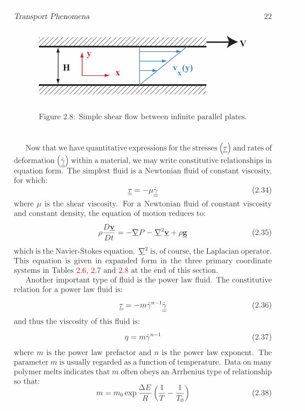
For simple shearing flows, such as steady shear between infinite parallelplates indicated in Figure 2.8, γ reduces to:
γ =
0 1 0
1 0 00 0 0
γ (2.32)
where γ is the shear rate. The shear rate is a scalar related to the secondinvariant of the rate of deformation tensor:
γ =
√1
2
(γ:γ
)(2.33)
Transport Phenomena 22
V
Hx
y
v (y)x
Figure 2.8: Simple shear flow between infinite parallel plates.
Now that we have quantitative expressions for the stresses(τ)
and rates of
deformation(γ
)within a material, we may write constitutive relationships in
equation form. The simplest fluid is a Newtonian fluid of constant viscosity,for which:
τ = −µγ (2.34)
where µ is the shear viscosity. For a Newtonian fluid of constant viscosityand constant density, the equation of motion reduces to:
ρDv
Dt= −∇P −∇2v + ρg (2.35)
which is the Navier-Stokes equation. ∇2 is, of course, the Laplacian operator.This equation is given in expanded form in the three primary coordinatesystems in Tables 2.6, 2.7 and 2.8 at the end of this section.
Another important type of fluid is the power law fluid. The constitutiverelation for a power law fluid is:
τ = −mγn−1γ (2.36)
and thus the viscosity of this fluid is:
η = mγn−1 (2.37)
where m is the power law prefactor and n is the power law exponent. Theparameter m is usually regarded as a function of temperature. Data on manypolymer melts indicates that m often obeys an Arrhenius type of relationshipso that:
m = m0 exp∆E
R
(1
T− 1
T0
)(2.38)

Transport Phenomena 23
where m0 is the value of m at T0, ∆E is the flow activation energy, R is thegas constant, and the temperature must be expressed in degrees Kelvin.
2.3.3 Boundary Conditions
In addition to the conservation and constitutive equations, initial and bound-ary conditions are required in order to solve a flow problem.
1. Solid-Fluid Interfaces
(a) The Slip Condition. By far, the most common assumption atsolid-fluid boundaries is the no-slip assumption, which asserts sim-ply that there is no relative motion between the two phases at theinterface:
vfluid = vsolid at the boundary . (2.39)
There are conditions under which it is believed that slip takes placebetween a fluid and solid, especially at high shear rates. Slip atthe wall is believed to occur at high flow rates, for example, inthe melt fracture regime of die extrusion. The melt fracture mayin fact be due to an intermittent slip-stick phenomena related tothe viscoelastic nature of the material. Various different modelsfor interfacial slip have appeared in the literature.
(b) Solid Penetrability. In the vast majority of cases, the fluid isassumed not to penetrate the surface of the solid. The equationgiven immediately above accurately implements this. If there ispenetration of the solid by the fluid, due perhaps to porosity, thefluid velocity at the interface is usually separated into normal andtangential components.
2. Fluid-Fluid Interfaces In this case there are four types of boundaryconditions that must be specified.
(a) The Slip Condition. The same no-slip assumption describedabove is typically assumed for fluid-fluid interfaces. This meansthat there is continuity of the tangential velocities at the interface.
vfluidA = vfluidB at the boundary . (2.40)
There are exceptions to its applicability.
Transport Phenomena 24
(b) Interface Penetrability. In the vast majority of cases, the fluidsare assumed not to penetrate across the interface. Similar com-ments apply as for the fluid-solid interface. The equation givendirectly above implements in impenetrable boundary condition,establishing the continuity of normal velocities at the interface.
(c) Balance of Shear Stresses at the Interface. The assumption isusually made that the shear stresses are continuous across theinterface:
τfluidA
= τfluidB
at the boundary . (2.41)
There are very few exceptions to this. One notable one would bethe case where the interface itself is considered a membrane withsome elastic properties.
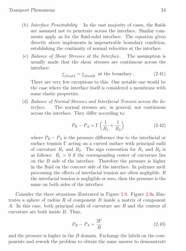
(d) Balance of Normal Stresses and Interfacial Tension across the In-terface. The normal stresses are, in general, not continuousacross the interface. They differ according to:
PB − PA = Γ(
1
R1
+1
R2
)(2.42)
where PB − PA is the pressure difference due to the interfacial orsurface tension Γ acting on a curved surface with principal radiiof curvature R1 and R2. The sign convention for R1 and R2 isas follows: Ri > 0 if the corresponding center of curvature lieson the B side of the interface. Therefore the pressure is higherin the fluid on the concave side of the interface. In polymer meltprocessing the effects of interfacial tension are often negligible. Ifthe interfacial tension is negligible or zero, then the pressure is thesame on both sides of the interface.
Consider the three situations illustrated in Figure 2.9. Figure 2.9a illus-trates a sphere of radius R of component B inside a matrix of componentA. In this case, both principal radii of curvature are R and the centers ofcurvature are both inside B. Thus,
PB − PA =2Γ
R(2.43)
and the pressure is higher in the B domain. Exchange the labels on the com-ponents and rework the problem to obtain the same answer to demonstrate

Transport Phenomena 25
the significance of the sign convention. Figure 2.9b illustrates a cylinder ofradius R and infinite length of component B inside a matrix of component A.In this case, one principal radii of curvature is R and the other is ∞. Thus,the pressure inside the cylinder is Γ/R larger than that outside. Figure 2.9cillustrates a B domain of complex shape inside a A matrix. In this case,there are no global principal radii of curvature; instead, the radii are poten-tially different at each location on the interface. Thus, the pressure differenceacross the interface due to interfacial tension is potentially different at eachlocation. What implications does this have for interfacial tension generatedflows? What implications does this have for the solution of a flow problemwith unusually shaped domains?
(a) (b) (c)
A
B
AA
BB
Figure 2.9: Various shapes of a fluid domain inside a matrix.
2.3.4 Example: Die Flow in Film Casting
Casting is commonly used to manufacture films or sheets of thermoplasticssuch as polyolefins, polyesters, and nylons. A single screw extruder meltsthe polymer and builds the pressure required to pump it through a die inorder to establish the geometry of the film or sheet. The molten materialis then cooled in its final form. The cross-section of a simple film die isshown in Figure 2.10. This figure approximates the die flow as a pressuredriven between parallel plates. The pressure difference responsible for theflow is the difference between the pressures at the entrance to and exit fromthe die, ∆P = P2 − P1. We are interested specifically in the relationshipbetween this pressure difference and the flow rate of polymer through thedie. The flow rate is, of course, closely related to the production rate of themanufacturing operation. In addition, we may be interested in the velocity

Transport Phenomena 26
field so that we can understand the stresses and deformation rates that thematerial experiences as it moves through the process. Designers of the dieitself will want to know the forces exerted by the flowing polymer on the dieto ensure that it is mechanically robust enough the contain the flow withoutdeforming.
H
x
y
z
CL
P1
P2
L
Figure 2.10: Cross-section of a film casting die.
Consider the well developed, steady-state pressure driven flow of an in-compressible power law fluid through the die. By describing the flow as “welldeveloped,” we mean that we will consider the flow to be that between paral-lel plates throughout the entire flow regime under consideration. In actuality,there will be some rearrangement of the flow as it enters the die from the ex-truder; there will also be some disruption of the flow as it exits the end of thedie into the open air. However, these entrance and exit effects are neglectedhere. By describing the flow as “steady-state,” we mean that all aspects ofthe flow are time independent. Film casting manufacturing operations arerun as close to steady-state as is feasible in order to produce a uniform filmthickness; however, there are small time dependent fluctuations in even thebest of production lines.
These notes will also often make the (unstated) assumption that the flowunder consideration is laminar and well ordered. This means that the mate-rial flow can be considered as being comprised of layers of fluid which slidepast each other. (Imagine these layers as individual playing cards if you wereshearing a deck of cards.) The counterpart of laminar flow is turbulent flow.However, the high viscosities of polymer melts nearly always prevent turbu-lence. The transition between laminar and turbulent flow in a flow between
Transport Phenomena 27
parallel plates is governed by the Reynolds number:
Re =HV ρ
µ(2.44)
where V is a representative velocity. A typical film casting operation mighthave a Reynolds number around 0.001, very much below that required fortransition to turbulence.
Clearly the rectangular coordinate system is most convenient for analysisof this problem. We may immediately conclude from the symmetry of theproblem that there is no dependence of any variable on the z-coordinate, all∂∂z
= 0. In addition, because this is a steady-state flow, all ∂∂t
= 0. It is alsoclear that vz = 0, vy = 0, and in terms of the velocities we are interestedonly in vx = vx(y). (Why? Check these conclusions for consistency using thecontinuity equation.) Since the effect of gravity is negligible here, we alsohave P = P (x) only.
On the basis of the results above, the x-component of the equation ofmotion reduces to:
0 = −dP
dx−
(∂τxx
∂x+
∂τyx
∂y
). (2.45)
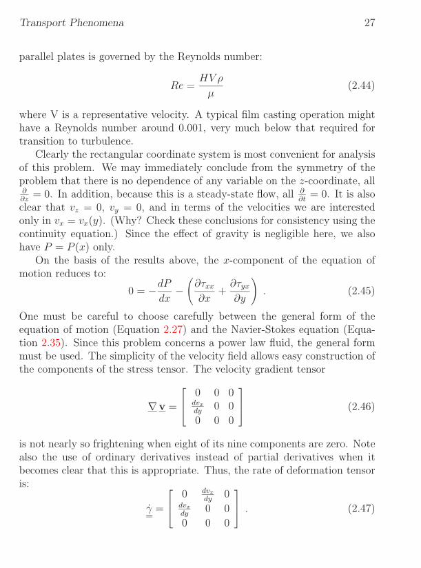
One must be careful to choose carefully between the general form of theequation of motion (Equation 2.27) and the Navier-Stokes equation (Equa-tion 2.35). Since this problem concerns a power law fluid, the general formmust be used. The simplicity of the velocity field allows easy construction ofthe components of the stress tensor. The velocity gradient tensor
∇v =
0 0 0dvx
dy0 0
0 0 0
(2.46)
is not nearly so frightening when eight of its nine components are zero. Notealso the use of ordinary derivatives instead of partial derivatives when itbecomes clear that this is appropriate. Thus, the rate of deformation tensoris:
γ =
0 dvx
dy0
dvx
dy0 0
0 0 0
. (2.47)

Transport Phenomena 28
Based on the constitutive equation for a power law fluid (Equation 2.36) andthe definition of the shear rate (Equation 2.33), we obtain τxx = 0 and
τxy = τyx = −mγn−1 dvx
dy(2.48)
where
γ =
∣∣∣∣∣dvx
dy
∣∣∣∣∣ . (2.49)
The absolute value has been used because the shear rate in Equation 2.33 isspecifically the positive square root.
The equation of motion may thus be rearranged to:
dP
dx= m
d
dy
[γn−1dvx
dy
]. (2.50)
The most direct procedure for solution of this equation is to recognize thatthe left hand side is a function of x only while the right hand side is a functionof y only. In order for the equality to hold throughout the entire flow domain,each side must be equal to some constant, C1. Thus,
dP
dx= C1 . (2.51)
Integration and application of the appropriate boundary conditions yields anexplicit expression for the pressure:
P (x) = P2 − ∆Px
L. (2.52)
This result may now be substituted into the other side of the original differ-ential equation:
md
dy
[γn−1dvx
dy
]= −∆P
L(2.53)
allowing another integration:
∣∣∣∣∣dvx
dy
∣∣∣∣∣n−1
dvx
dy= −∆P
mLy + C2 (2.54)
In order to simplify the solution, we will now take advantage of the sym-metry of the problem and limit our analysis to the regime y ≤ 0. Since
Transport Phenomena 29
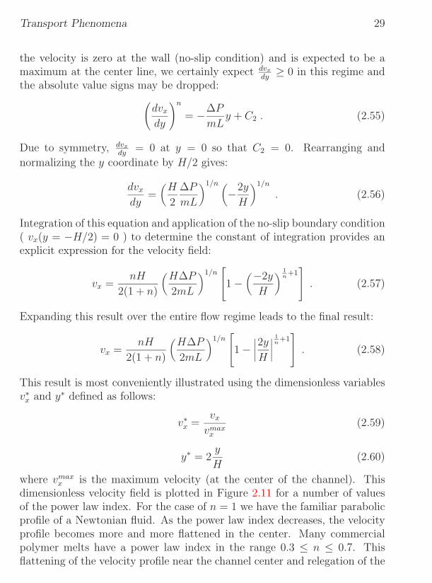
the velocity is zero at the wall (no-slip condition) and is expected to be amaximum at the center line, we certainly expect dvx
dy≥ 0 in this regime and
the absolute value signs may be dropped:(dvx
dy
)n
= −∆P
mLy + C2 . (2.55)
Due to symmetry, dvx
dy= 0 at y = 0 so that C2 = 0. Rearranging and
normalizing the y coordinate by H/2 gives:
dvx
dy=
(H
2
∆P
mL
)1/n (−2y
H
)1/n
. (2.56)
Integration of this equation and application of the no-slip boundary condition( vx(y = −H/2) = 0 ) to determine the constant of integration provides anexplicit expression for the velocity field:
vx =nH
2(1 + n)
(H∆P
2mL
)1/n1 −
(−2y
H
) 1n
+1 . (2.57)
Expanding this result over the entire flow regime leads to the final result:
vx =nH
2(1 + n)
(H∆P
2mL
)1/n1 −
∣∣∣∣2yH∣∣∣∣
1n
+1 . (2.58)
This result is most conveniently illustrated using the dimensionless variablesv∗
x and y∗ defined as follows:
v∗x =
vx
vmaxx
(2.59)
y∗ = 2y
H(2.60)
where vmaxx is the maximum velocity (at the center of the channel). This
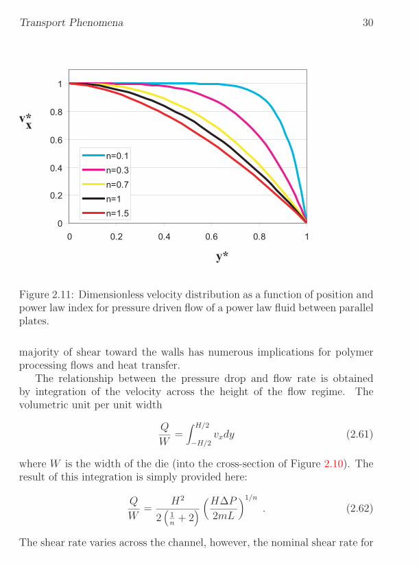
dimensionless velocity field is plotted in Figure 2.11 for a number of valuesof the power law index. For the case of n = 1 we have the familiar parabolicprofile of a Newtonian fluid. As the power law index decreases, the velocityprofile becomes more and more flattened in the center. Many commercialpolymer melts have a power law index in the range 0.3 ≤ n ≤ 0.7. Thisflattening of the velocity profile near the channel center and relegation of the
Transport Phenomena 30
0
0.2
0.4
0.6
0.8
1
0 0.2 0.4 0.6 0.8 1
n=0.1
n=0.3
n=0.7
n=1
n=1.5
y*
v*x
Figure 2.11: Dimensionless velocity distribution as a function of position andpower law index for pressure driven flow of a power law fluid between parallelplates.
majority of shear toward the walls has numerous implications for polymerprocessing flows and heat transfer.
The relationship between the pressure drop and flow rate is obtainedby integration of the velocity across the height of the flow regime. Thevolumetric unit per unit width
Q
W=
∫ H/2
−H/2vxdy (2.61)
where W is the width of the die (into the cross-section of Figure 2.10). Theresult of this integration is simply provided here:
Q
W=
H2
2(
1n
+ 2) (
H∆P
2mL
)1/n
. (2.62)
The shear rate varies across the channel, however, the nominal shear rate for
Transport Phenomena 31
this type of flow is usually taken to be the shear rate at the wall:
dvx
dy
∣∣∣∣∣y=H/2
=(
H
2
∆P
mL
)1/n
. (2.63)
In addition, we are interested in the force/unit area exerted by the flowingpolymer melt on the walls of the channel. There are several methods ofcalculating this; however, we will use this example to illustrate use of thetotal stress tensor for this purpose. All of the components of π have alreadybeen determined:
π =
P (x) −m∣∣∣dvx
dy
∣∣∣n−1dvx
dy0
−m∣∣∣dvx
dy
∣∣∣n−1dvx
dyP (x) 0
0 0 P (x)
(2.64)
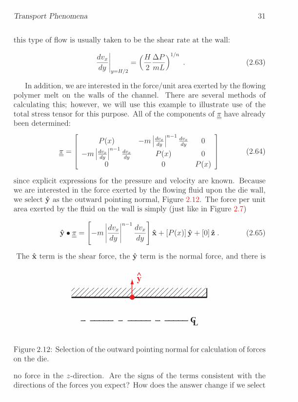
since explicit expressions for the pressure and velocity are known. Becausewe are interested in the force exerted by the flowing fluid upon the die wall,we select y as the outward pointing normal, Figure 2.12. The force per unitarea exerted by the fluid on the wall is simply (just like in Figure 2.7)
y • π =
−m
∣∣∣∣∣dvx
dy
∣∣∣∣∣n−1
dvx
dy
x + [P (x)] y + [0] z . (2.65)
The x term is the shear force, the y term is the normal force, and there is
CL
y
Figure 2.12: Selection of the outward pointing normal for calculation of forceson the die.
no force in the z-direction. Are the signs of the terms consistent with thedirections of the forces you expect? How does the answer change if we select

Transport Phenomena 32
−y as the outward pointing normal at the lower lip of the die? How wouldyou obtain the total force on the die surfaces rather than just the force perunit area? How would the approach be different if we were to calculate theforce exerted by the die surface on the polymer melt? Can you see a fasterway to calculate these forces based on the simple geometry of this particularproblem?
2.3.5 Example: Blowing of a Cylindrical Parison
Blow molding is a shaping operation commonly used with amorphous poly-mers and rapidly crystallizing semicrystalline polymers. A hot cylindricalparison is inflated against a cold mold in order to form a hollow object suchas a bottle. In the central region of the object, the process can often beaccurately approximated as the inflation of a cylindrical shell.
Consider the inflation of a cylindrical shell of polymer melt, as illustratedin Figure 2.13. The cylindrical shell is initially of radius R0 and wall thicknessH0. Starting at time zero, it is inflated by the application of air pressureP1(t) at the center of the cylindrical “bubble.” Subsequently, the radiusR(t) increases as a function of time and the wall thickness H(t) decreases.Throughout the process, assume that the cylindrical shape is maintained andthe length of the cylinder is constant at L. At all times the radius is muchlarger than the wall thickness, R(t) H(t); in addition, the length of thecylinder is much larger than the radius, L R(t). The pressure on theoutside of the cylindrical shell is constant at Patm. The polymer contactsthe mold wall at the final radius Rf . The density of the polymer melt isconstant.
As the cylindrical shell is inflated, the pressure P1(t) is adjusted so thatthe inflation velocity dR(t)/dt is constant throughout at a value of V0. Whatis R(t)? What is H(t)? What is the velocity distribution within the expand-ing cylindrical shell of polymer? What type of flow is this? What is thedeformation rate as a function of time?
Assume that the polymer melt is a Newtonian fluid of constant viscosityµ. What is the blowing pressure P1(t) required to produce the specifieddeformation? [Hint: inertial effects and interfacial tension are negligible.]
Suppose instead that the polymer is a shear thinning fluid or a shearthickening fluid. How would you expect P1(t) for these types of material tocompare to that for a Newtonian fluid?
The geometry of the problem is illustrated in Figure 2.14. A cylindrical

Transport Phenomena 33
Ro
owall thickness H
L
R(t)
wall thickness H(t)
PatmP (t)1
Figure 2.13: Idealization of the blow molding process as the inflation of acylindrical parison of polymer melt.
coordinate system is used in order to take advantage of the symmetry of theproblem. On the basis of the assumptions and symmetry we may immediatelyconclude: vz = 0 and vθ = 0. There is no θ or z dependence of any variables.We are thus interested in determining within the polymer melt the variables:vr = vr(r, t) and P = P (r, t).
R(t)
H(t)
Patm P (t)
1r
zR(t) >> H(t)
L(t) >> R(t)
ρ = constant
cylindrical coord.
Figure 2.14: Sketch of problem geometry.
A constant inflation velocity means that: dR(t)dt
= V0 = constant, whichcan be integrated to obtain: R = R0 + V0t. Since the polymer is incom-pressible, the total volume of the cylindrical shell must remain constant.Using H(t) R(t) we may estimate: V olume ∼= 2πR0H0L = 2πR(t)H(t)L,

Transport Phenomena 34
yielding
H(t) = H0R0
R0 + V0t. (2.66)
The equation of continuity in cylindrical coordinates for an incompressiblefluid with zero θ and z velocities reduces to:
∂
∂r(rvr) +
1
r= 0 . (2.67)
This can be immediately integrated to obtain: vr = C(t)r
for some functionC(t). (Why is the “constant” of integration potentially a function of time?)The boundary condition at the inner radius is:
R(t)vr|R(t) = R(t)dR(t)
dt= R(t)V0 . (2.68)
Application of this boundary condition yields:
vr = V0R0 + V0t
r. (2.69)
The velocity gradient tensor for the current flow is:
∇v =
∂vr
∂r0 0
0vr
r0
0 0 0
.
Substitution of the velocity field obtained above yields the rate of deformationtensor:
γ =
−2V0
R0 + V0t
r20 0
0 2V0R0 + V0t
r20
0 0 0
.
This is an extensional flow since the only nonzero components of the rate ofdeformation tensor are along the diagonal. The scalar shear rate is:
γ = 2V0R0 + V0t
r2. (2.70)
Transport Phenomena 35
1P (t)
Patm
t0
4 µ V Ho o
oR2
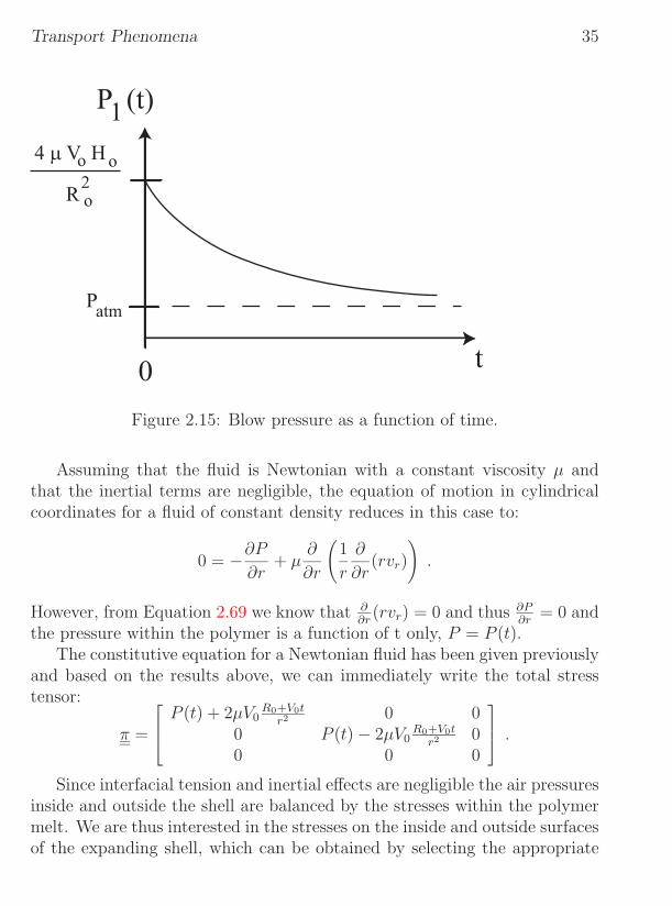
Figure 2.15: Blow pressure as a function of time.
Assuming that the fluid is Newtonian with a constant viscosity µ andthat the inertial terms are negligible, the equation of motion in cylindricalcoordinates for a fluid of constant density reduces in this case to:
0 = −∂P
∂r+ µ
∂
∂r
(1
r
∂
∂r(rvr)
).
However, from Equation 2.69 we know that ∂∂r
(rvr) = 0 and thus ∂P∂r
= 0 andthe pressure within the polymer is a function of t only, P = P (t).
The constitutive equation for a Newtonian fluid has been given previouslyand based on the results above, we can immediately write the total stresstensor:
π =
P (t) + 2µV0
R0+V0tr2 0 0
0 P (t) − 2µV0R0+V0t
r2 00 0 0
.
Since interfacial tension and inertial effects are negligible the air pressuresinside and outside the shell are balanced by the stresses within the polymermelt. We are thus interested in the stresses on the inside and outside surfacesof the expanding shell, which can be obtained by selecting the appropriate

Transport Phenomena 36
components of the total stress tensor. At the inner surface we obtain:
P1(t) = P (t) + 2µV0R0 + V0t
R2(t)
while at the outer surface
Patm(t) = P (t) + 2µV0R0 + V0t
[R(t) + H(t)]2.
Subtracting these and recognizing that H(t) R(t) leads to:
P1(t) − Patm =4µV0H(t)
R2(t)=
4µV0H0R0
[R0 + V0t]3. (2.71)
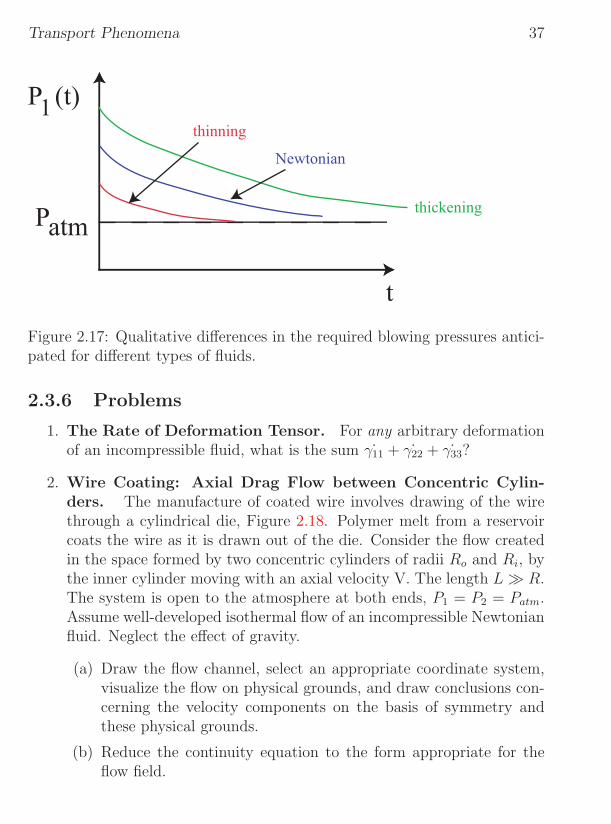
The required blowing pressure as a function of time is plotted in Figure 2.15.For non-Newtonian fluids the shear rate still changes according to Equa-
tion 2.70 (Why?). Thus, the deformation rate decreases approximately as1/R. As a function of shear rate, three fluids of the same zero shear viscositywill qualitatively behave as illustrated in Figure 2.16. The resulting pressureeffects are shown in Figure 2.17.
η
γ.
Newtonian
shear thinning
shear thickening
Figure 2.16: Qualitative behavior of three fluids with the same zero shearviscosity.
Transport Phenomena 37
1P (t)
Patm
t
Newtonian
thinning
thickening
Figure 2.17: Qualitative differences in the required blowing pressures antici-pated for different types of fluids.
2.3.6 Problems
1. The Rate of Deformation Tensor. For any arbitrary deformationof an incompressible fluid, what is the sum ˙γ11 + ˙γ22 + ˙γ33?
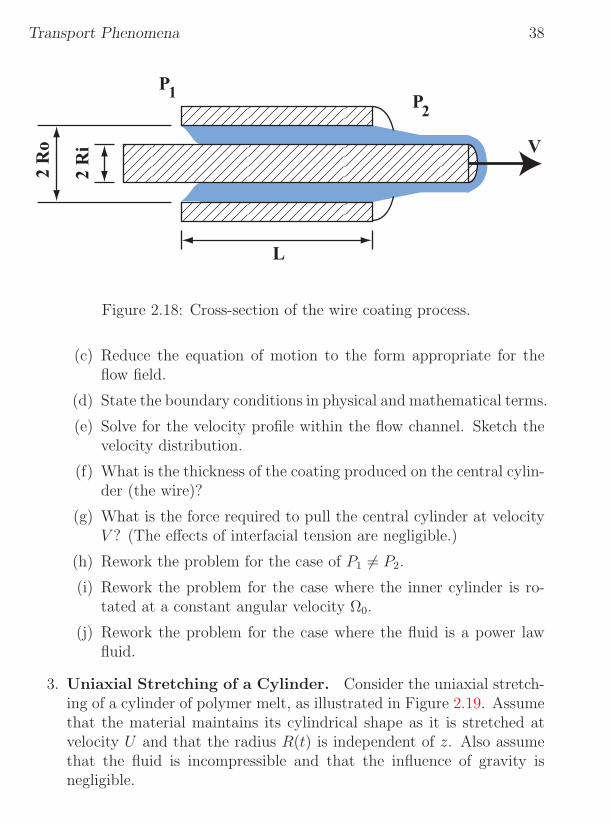
2. Wire Coating: Axial Drag Flow between Concentric Cylin-ders. The manufacture of coated wire involves drawing of the wirethrough a cylindrical die, Figure 2.18. Polymer melt from a reservoircoats the wire as it is drawn out of the die. Consider the flow createdin the space formed by two concentric cylinders of radii Ro and Ri, bythe inner cylinder moving with an axial velocity V. The length L R.The system is open to the atmosphere at both ends, P1 = P2 = Patm.Assume well-developed isothermal flow of an incompressible Newtonianfluid. Neglect the effect of gravity.
(a) Draw the flow channel, select an appropriate coordinate system,visualize the flow on physical grounds, and draw conclusions con-cerning the velocity components on the basis of symmetry andthese physical grounds.
(b) Reduce the continuity equation to the form appropriate for theflow field.
Transport Phenomena 382 R
o
2 R
iP
1P
2
L
V
Figure 2.18: Cross-section of the wire coating process.
(c) Reduce the equation of motion to the form appropriate for theflow field.
(d) State the boundary conditions in physical and mathematical terms.
(e) Solve for the velocity profile within the flow channel. Sketch thevelocity distribution.
(f) What is the thickness of the coating produced on the central cylin-der (the wire)?
(g) What is the force required to pull the central cylinder at velocityV ? (The effects of interfacial tension are negligible.)
(h) Rework the problem for the case of P1 = P2.
(i) Rework the problem for the case where the inner cylinder is ro-tated at a constant angular velocity Ω0.
(j) Rework the problem for the case where the fluid is a power lawfluid.
3. Uniaxial Stretching of a Cylinder. Consider the uniaxial stretch-ing of a cylinder of polymer melt, as illustrated in Figure 2.19. Assumethat the material maintains its cylindrical shape as it is stretched atvelocity U and that the radius R(t) is independent of z. Also assumethat the fluid is incompressible and that the influence of gravity isnegligible.

Transport Phenomena 39
L(t)
U
R(t)
r
z
Figure 2.19: Stretching of a cylinder of fluid.
(a) Using the continuity equation, show that the velocity field withinthe stretching cylinder is:
vr = − Ur
2L(t); vz =
Uz
L(t)
What is R(t)?
(b) Give the components of γ for this flow. What kind of flow field is
this?
(c) Neglecting surface tension and inertial effects, calculate the forceF required to pull the cylinder for a Newtonian fluid of viscosityµ.
(d) If instead, F is a constant (and thus U is a function of time), howdoes L change with time?
(e) How must L be programmed, i.e. give L(t), such that the com-ponents of γ are independent of time. Is this result true only for
Newtonian fluids? Why or why not?
(f) Neglecting surface tension and inertial effects, calculate the forceF (t) required to pull the cylinder at constant velocity U for apower law fluid of power law exponent n and prefactor m. Ifinstead F is constant, how does L change with time?
4. Biaxial Stretching of a Sheet. Biaxial orientation of polymer sheetor film is commonly used to improve mechanical properties. Consider

Transport Phenomena 40
the biaxial stretching of a sheet of polymer melt, as shown in Figure2.20. The sheet is initially square, with the same width and length,L0, and a thickness of H0. Starting at time zero, a series of travel-ling clamps on all four edges of the sheet simultaneously stretch thesheet at a constant velocity V in the x and y directions. The sheet isfree to deform in the thickness direction, which is open to the atmo-sphere. The sheet maintains its square shape as it is deformed, withwidth and length L(t) and thickness H(t). Assume that the materialis incompressible and that the influence of gravity is negligible.
L(t)
H(t)
x
yz
Figure 2.20: Simultaneous stretching of a square sheet in two directions.
(a) Using the equation of continuity, show that the velocity fieldwithin the stretching sheet is:
vx = 2Vx
L(t); vy = 2V
y
L(t); vz = −4V
z
L(t)
What is H(t)?
(b) Give the components of γ for this flow. What kind of flow field is
this?
(c) Neglecting surface tension and inertial effects, calculate the forceF (t) that the clamps must exert on each edge of the sheet inorder to impose the specified deformation if the polymer melt isa Newtonian fluid of constant viscosity µ.
(d) If instead F is held constant at F0 (and thus V is a function oftime), how does H change with time?
Transport Phenomena 41
(e) How must V be programmed, i.e. give V (t) such that the com-ponents of γ are independent of time? Is this result true only for
Newtonian fluids? Why or why not?
(f) Neglecting surface tension and inertial effects, calculate the forceF (t) required to stretch the sheet at constant velocity V for apower law fluid of power law exponent n and prefactor m. Ifinstead F is a constant, how does H change with time?
2.3.7 Further Reading
Excellent derivations and explanations of the equations of continuity andmotion may be found in:
• R.B. Bird, W.E. Stewart, E.N. Lightfoot Transport Phenomena,John Wiley and Sons, New York (1960).
• R.B. Bird, R.C. Armstrong, O. Hassager, Dynamics of PolymericLiquids, Vol. 1, John Wiley and Sons, New York (1987).
Numerous illustrative problems, some with solutions may be found in:
• W.F. Hughes, J.A. Brighton, Fluid Dynamics, Schaum’s Outline Se-ries, McGraw-Hill Book Company (1967).
• G.E. Mase, Continuum Mechanics, Schaum’s Outline Series, McGraw-Hill Book Company (1970).

Transport Phenomena 42
2.3.8 Expanded forms of the Equation of Motion
ρ
(∂vx
∂t+ vx
∂vx
∂x+ vy
∂vx
∂y+ vz
∂vx
∂z
)= −∂P
∂x−
(∂τxx
∂x+
∂τyx
∂y+
∂τzx
∂z
)+ ρgx
(2.72)
ρ
(∂vy
∂t+ vx
∂vy
∂x+ vy
∂vy
∂y+ vz
∂vy
∂z
)= −∂P
∂y−
(∂τxy
∂x+
∂τyy
∂y+
∂τzy
∂z
)+ ρgy
(2.73)
ρ
(∂vz
∂t+ vx
∂vz
∂x+ vy
∂vz
∂y+ vz
∂vz
∂z
)= −∂P
∂z−
(∂τxz
∂x+
∂τyz
∂y+
∂τzz
∂z
)+ ρgz
(2.74)
Table 2.3: The equation of motion in rectangular coordinates.
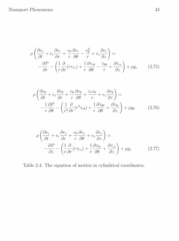
Transport Phenomena 43
ρ
(∂vr
∂t+ vr
∂vr
∂r+
vθ
r
∂vr
∂θ− v2
θ
r+ vz
∂vr
∂z
)=
−∂P
∂r−
(1
r
∂
∂r(rτrr) +
1
r
∂τrθ
∂θ− τθθ
r+
∂τrz
∂z
)+ ρgr (2.75)
ρ
(∂vθ
∂t+ vr
∂vθ
∂r+
vθ
r
∂vθ
∂θ+
vrvθ
r+ vz
∂vθ
∂z
)=
−1
r
∂P
∂θ−
(1
r2
∂
∂r(r2τrθ) +
1
r
∂τθθ
∂θ+
∂τθz
∂z
)+ ρgθ (2.76)
ρ
(∂vz
∂t+ vr
∂vz
∂r+
vθ
r
∂vz
∂θ+ vz
∂vz
∂z
)=
−∂P
∂z−
(1
r
∂
∂r(rτrz) +
1
r
∂τθz
∂θ+
∂τzz
∂z
)+ ρgz (2.77)
Table 2.4: The equation of motion in cylindrical coordinates.

Transport Phenomena 44
ρ
(∂vr
∂t+ vr
∂vr
∂r+
vθ
r
∂vr
∂θ+
vφ
r sin θ
∂vr
∂φ− v2
θ + v2φ
r
)=
−∂P
∂r−
(1
r2
∂
∂r(r2τrr) +
1
r sin θ
∂
∂θ(τrθ sin θ)
+1
r sin θ
∂τrφ
∂φ− τθθ + τφφ
r
)+ ρgr (2.78)
ρ
(∂vθ
∂t+ vr
∂vθ
∂r+
vθ
r
∂vθ
∂θ+
vφ
r sin θ
∂vθ
∂φ+
vrvθ
r− v2
φ cot θ
r
)=
−1
r
∂P
∂θ−
(1
r2
∂
∂r(r2τrθ) +
1
r sin θ
∂
∂θ(τθθ sin θ)
+1
r sin θ
∂τθφ
∂φ+
τrθ
r− cot θ
rτφφ
)+ ρgθ (2.79)
ρ
(∂vφ
∂t+ vr
∂vφ
∂r+
vθ
r
∂vφ
∂θ+
vφ
r sin θ
∂vφ
∂φ+
vφvr
r+
vθvφ
rcot θ
)=
− 1
r sin θ
∂P
∂φ−
(1
r2
∂
∂r(r2τrφ) +
1
r
∂τθφ
∂θ+
1
r sin θ
∂τφφ
∂φ
+τrφ
r+
2 cot θ
rτθφ
)+ ρgφ (2.80)
Table 2.5: The equation of motion in spherical coordinates.

Transport Phenomena 45
ρ
(∂vx
∂t+ vx
∂vx
∂x+ vy
∂vx
∂y+ vz
∂vx
∂z
)= −∂P
∂x+µ
(∂2vx
∂x2+
∂2vx
∂y2+
∂2vx
∂z2
)+ρgx
(2.81)
ρ
(∂vy
∂t+ vx
∂vy
∂x+ vy
∂vy
∂y+ vz
∂vy
∂z
)= −∂P
∂y+µ
(∂2vy
∂x2+
∂2vy
∂y2+
∂2vy
∂z2
)+ρgy
(2.82)
ρ
(∂vz
∂t+ vx
∂vz
∂x+ vy
∂vz
∂y+ vz
∂vz
∂z
)= −∂P
∂z+µ
(∂2vz
∂x2+
∂2vz
∂y2+
∂2vz
∂z2
)+ρgz
(2.83)
Table 2.6: The Navier-Stokes equation in rectangular coordinates, for fluidsof constant density ρ and constant viscosity µ.

Transport Phenomena 46
ρ
(∂vr
∂t+ vr
∂vr
∂r+
vθ
r
∂vr
∂θ− v2
θ
r+ vz
∂vr
∂z
)=
−∂P
∂r+ µ
[∂
∂r
(1
r
∂
∂r(rvr)
)+
1
r2
∂2vr
∂θ2− 2
r2
∂vθ
∂θ+
∂2vr
∂z2
]+ ρgr(2.84)
ρ
(∂vθ
∂t+ vr
∂vθ
∂r+
vθ
r
∂vθ
∂θ+
vrvθ
r+ vz
∂vθ
∂z
)=
−1
r
∂P
∂θ+ µ
[∂
∂r
(1
r
∂
∂r(rvθ)
)+
1
r2
∂2vθ
∂θ2
+2
r2
∂vr
∂θ+
∂2vθ
∂z2
]+ ρgθ (2.85)
ρ
(∂vz
∂t+ vr
∂vz
∂r+
vθ
r
∂vz
∂θ+ vz
∂vz
∂z
)=
−∂P
∂z+ µ
[1
r
∂
∂r
(r∂vz
∂r
)+
1
r2
∂2vz
∂θ2+
∂2vz
∂z2
]+ ρgz (2.86)
Table 2.7: The Navier-Stokes equation in cylindrical coordinates, for fluidsof constant density ρ and constant viscosity µ.
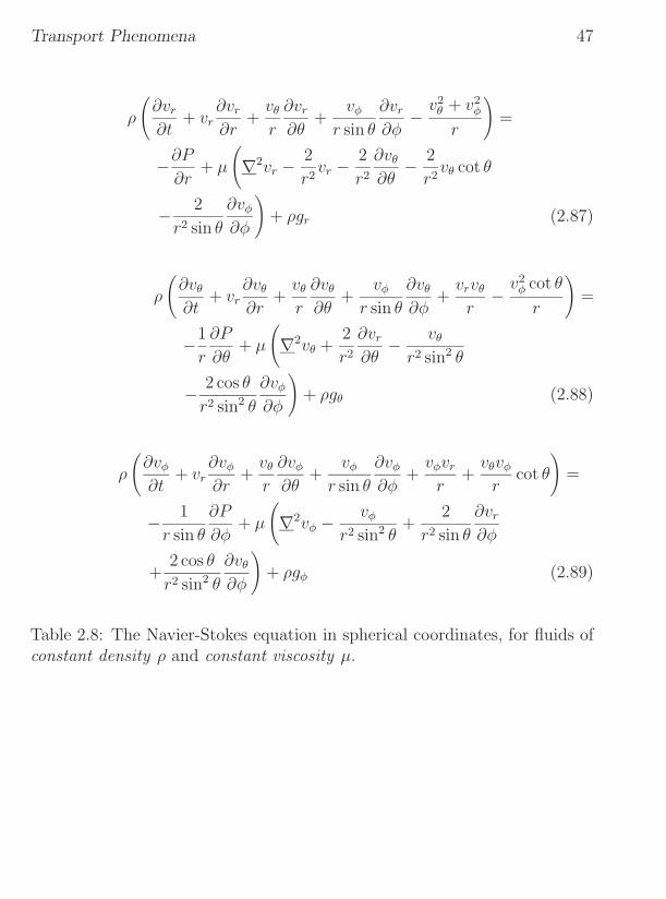
Transport Phenomena 47
ρ
(∂vr
∂t+ vr
∂vr
∂r+
vθ
r
∂vr
∂θ+
vφ
r sin θ
∂vr
∂φ− v2
θ + v2φ
r
)=
−∂P
∂r+ µ
(∇2vr − 2
r2vr − 2
r2
∂vθ
∂θ− 2
r2vθ cot θ
− 2
r2 sin θ
∂vφ
∂φ
)+ ρgr (2.87)
ρ
(∂vθ
∂t+ vr
∂vθ
∂r+
vθ
r
∂vθ
∂θ+
vφ
r sin θ
∂vθ
∂φ+
vrvθ
r− v2
φ cot θ
r
)=
−1
r
∂P
∂θ+ µ
(∇2vθ +
2
r2
∂vr
∂θ− vθ
r2 sin2 θ
− 2 cos θ
r2 sin2 θ
∂vφ
∂φ
)+ ρgθ (2.88)
ρ
(∂vφ
∂t+ vr
∂vφ
∂r+
vθ
r
∂vφ
∂θ+
vφ
r sin θ
∂vφ
∂φ+
vφvr
r+
vθvφ
rcot θ
)=
− 1
r sin θ
∂P
∂φ+ µ
(∇2vφ − vφ
r2 sin2 θ+
2
r2 sin θ
∂vr
∂φ
+2 cos θ
r2 sin2 θ
∂vθ
∂φ
)+ ρgφ (2.89)
Table 2.8: The Navier-Stokes equation in spherical coordinates, for fluids ofconstant density ρ and constant viscosity µ.

Transport Phenomena 48
Copyright 2001, PolymerProcessing.com.