2414 ieee transactions on biomedical engineering, … · parametric surface-source modeling and...

2414 IEEE TRANSACTIONS ON BIOMEDICAL ENGINEERING, VOL. 53, NO. 12, DECEMBER 2006

Parametric Surface-Source Modeling and EstimationWith Electroencephalography

Nannan Cao*, Student Member, IEEE, Imam Samil Yetik, Member, IEEE, Arye Nehorai, Fellow, IEEE,Carlos H. Muravchik, Senior Member, IEEE, and Jens Haueisen, Member, IEEE

Abstract—Electroencephalography (EEG) is an important toolfor studying the brain functions and is becoming popular in clinicalpractice. In this paper, we develop four parametric EEG modelsto estimate current sources that are spatially distributed on a sur-face. Our models approximate the source shape and extent explic-itly and can be applied to localize extended sources which are oftenencountered, e.g., in epilepsy diagnosis. We assume a realistic headmodel and solve the EEG forward problem using the boundary el-ement method. We present the source models with increasing de-grees of freedom, provide the forward solutions, and derive themaximum-likelihood estimates as well as Cramér-Rao bounds ofthe unknown source parameters. In order to evaluate the appli-cability of the proposed models, we first compare their estimationperformances with the dipole model’s using several known sourcedistributions. We then discuss the conditions under which we candistinguish between the proposed extended sources and the focaldipole using the generalized likelihood ratio test. We also applyour models to the electric measurements obtained from a phantombody in which an extended electric source is imbedded. We observethat the proposed model can capture the source extent informationsatisfactorily and the localization accuracy is better than the dipolemodel.

Index Terms—Cramér-Rao bounds, EEG, extended source mod-eling, likelihood ratio test.

I. INTRODUCTION

ELECTROENCEPHALOGRAPHY (EEG) is a noninvasivetechnique to analyze the spatial and temporal activities in

the brain. It has a high temporal resolution on the order of a fewmicroseconds and is applied in clinical practice (e.g., neurologyand psychiatry) [1] as well as basic neuroscience (e.g., in theinvestigation of primary sensory and motor functions or in theanalysis of cognition) [2]. The EEG forward problem describesthe distribution of electric potentials for given source locations

Manuscript received November 30, 2005; revised May 21, 2006. This workwas supported by the National Science Foundation (NSF) under Grant CCR-0105334. Asterisk indicates corresponding author.

*N. Cao is with the Department of Electrical and Systems Engineering, Wash-ington University, St. Louis, MO 63130 USA. She is also with the Bryan 201,Campus Box 1127, 1 Brookings Drive, St. Louis, MO 63130 USA (e-mail:[email protected]).

I.S. Yetik is with the Department of Electrical and Computer Engineering,Illinois Institute of Technology, Chicago, IL 60616 USA.

A. Nehorai is with the Department of Electrical and Systems Engineering,Washington University, St. Louis, MO 63130 USA.

C. H. Muravchik is with the Departamento de Electrotecnia, Facultad de In-genieria, Universidad Nacional de La Plata, Argentina.

J. Haueisen is with the Neurological University Hospital, Jena D-07743, Ger-many, and also with the Institute of Biomedical Engineering and Informatics,TU-Ilmenau, Ilmenau 98693, Germany.

Digital Object Identifier 10.1109/TBME.2006.883741

and signals, whereas the EEG inverse problem infers the under-lying activities from the measured potentials on the scalp. Theinverse problem is ill-posed, and prior constraints need to be ap-plied to obtain a unique solution [3].

Choosing an appropriate source model is an important stepin setting up the forward model. Most often, it is assumed thatthe source extent is small compared with its distances to the sen-sors and thus a current dipole is used to model it [4], [5]. Clearly,this approach is valid only if the electric activity is confined toa very small area. The current multipole expansion makes sys-tematic correction to the dipole model so that information (e.g.,the source spatial extent) independent of the basic dipole pa-rameters (i.e., dipole position and moment) can be extracted inthe order of significance [6], [7], but its performance would alsodegrade if the electric activities are spread over a large area. Fur-thermore, it is critical for both methods to have a correct esti-mate of the number of sources in order to get a correct inversesolution.

Different approaches have been proposed to model more ex-tended sources. The cortical patch methods divide the corticalsurface into small patches and describe the polarization of eachpatch by an associated current dipole [8]–[11]. Minimum norm(MN) based methods with anatomical and physiological con-straints are applied to estimate the source locations. The dis-tributed source imaging reconstructs the brain activities on a3-D grid where each point is considered as a possible locationof a current dipole [12], [13]. The inverse solutions also utilizethe MN criterion ( -norms with ), and they es-timate the moments of individual dipoles such that the sum ofthe norm of their moments and the fitting error is minimized.Both of these methods have the advantage of being able to esti-mate the number of active sources without any foreknowledge,but they also have certain problems. First, the MN-based so-lutions are in general highly underdetermined: the number ofunknowns is much more than the number of sensors and thusthere exist an infinite number of source distributions which canlead to exactly the same potential map. Therefore, regulariza-tion techniques [13], [14] or iterative focalization approaches[15], [16] are necessary to tackle this problem. Second, thereexist tradeoffs in performances depending on the definition ofthe norm: the minimum norm methods are faster to computethan the norms with , but they suffer from an artifi-cial “smearing” in the reconstructed source distribution; fornorms with close to 1, the “smearing” effect vanishes how-ever the method becomes very sensitive to noise [17]. All thesefactors need to be considered in order to deduce a reasonablesolution.

0018-9294/$20.00 © 2006 IEEE

CAO et al.: PARAMETRIC SURFACE-SOURCE MODELING AND ESTIMATION WITH EEG 2415

Recently, much work has been done on the cortical poten-tial imaging which is one of the high-resolution EEG imagingmodalities [18]–[20]. This method uses an explicit biophysicalmodel of the passive conducting properties of a head to decon-volve the measured scalp EEG into a cortical-surface potentialmap [18]. The estimated cortical potentials offer more spatialdetails than the scalp potentials since they are not affected bythe insulating skull layer.

In this paper, we present four parametric surface-sourcemodels for EEG assuming a realistic head model (RHM), basedon our previous work on EEG/MEG extended source modeling[21], [22]. Our method is a useful addition to the currentalgorithms. It differs with the above imaging techniques in thefollowing aspects. First, the source extent is directly parame-terized into the model and can be estimated, providing morespecific information. Second, we use basis function expansionin the forward models to exploit the prior information on thesource distribution, therefore, anatomical constraints (e.g.,the shape of the cortical surface) can be incorporated and thenumber of unknown parameters is greatly reduced too. We usethe boundary element method (BEM) to solve the quasi-staticMaxwell equations and formulate the EEG forward problem ina kernel-matrix form [23]. This structure facilitates the solutionof the inverse problem through decoupling the source locationparameters from the signals. We estimate the source parametersusing the maximum-likelihood (ML) method and derive theCramér-Rao bound (CRB) to evaluate the estimation perfor-mance [24], [25]. The CRB is a lower bound on the variance ofany unbiased estimator. It has the important features of beinguniversal and asymptotically tight; hence provides the bestestimation accuracy that can be expected from a certain model.In order to evaluate the applicability of our method, we firstcompare the performance of our models with that of the dipolemodel using several known source distributions. We use themean-squared error (MSE) as our model selection criterion. Wethen investigate the conditions under which our surface-sourcemodels and the focal dipole are distinguishable using thegeneralized likelihood ratio test (GLRT). Finally, we apply ourmodels to the electric measurements obtained from a phantombody in which an extended electric source is imbedded.

This paper is organized as follows. In Section II, we give abrief review of the RHM and BEM. In Section III we describethe surface-source models with increasing degrees of freedom,formulate the EEG forward models, and derive the ML estimatesof the unknown parameters. We discuss the CRBs in Section IVand present the numerical examples in Section V. Conclusionsare given in Section VI.

II. REALISTIC HEAD MODEL AND BOUNDARY

ELEMENT METHOD

Besides the source modeling as discussed in Section I,choosing a proper head model is another important issue inthe EEG forward problem. The simplest model is the homoge-neous spherical head model, where the head is considered as asphere with uniform conductivity [26]. This approach allowsan analytical solution to the EEG forward problem and thusis computationally efficient, but it results in low source local-ization accuracy. A multishell spherical model can improvethe performance by considering the head as several concentric

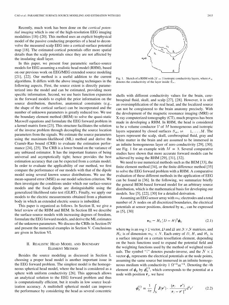
Fig. 1. Sketch of a RHM withM = 3 isotropic conductivity layers, where �denotes the conductivity of the layer inside S .

shells with different conductivity values for the brain, cere-brospinal fluid, skull, and scalp [27], [28]. However, it is stillan oversimplification of the real head, and the localized sourcecan not be coregistered to the brain anatomy precisely. Withthe development of the magnetic resonance imaging (MRI) orX-ray computerized tomography (CT), much progress has beenmade in developing a RHM. In RHM, the head is consideredto be a volume conductor of homogeneous and isotropiclayers separated by closed surfaces , . Thelayers represent the scalp, skull, cerebrospinal fluid, gray andwhite matter in the brain and are assumed to be immersed inan infinite homogeneous layer of zero conductivity [29], [30];see Fig. 1 for an example with . Several comparativestudies have shown that more accurate forward models can beachieved by using the RHM [29], [31], [32].

We need to use numerical methods such as the BEM [33], thefinite element method [34], or the finite difference method [35]to solve the EEG forward problem with a RHM. A comparativeevaluation of these different methods in the application of EEGcan be found in [36]. In the following, we summarize brieflythe general BEM-based forward model for an arbitrary sourcedistribution, which is the mathematical basis for developing ourmodels. See [5], [22], [30] for a detailed derivation.

Assuming an EEG sensor array with electrodes and a totalnumber of nodes on all discretized boundaries, the electricalpotentials at sensor positions, denoted by , can be expressedas [5], [30]

(2.1)

where is an vector, and are matrices, andis of dimension . Each entry of , , and is

a surface integral on a certain tessellation element, dependingon the basis functions used to expand the potential field andthe weighting functions used by the method of weighted resid-uals. The symbol “ ” denotes pseudo-inverse, and thevector represents the electrical potentials at the node points,assuming the same source but immersed in an infinite homoge-neous medium with conductivity 1 . Denoting the thelement of by , which corresponds to the potential at anode with position , we have

(2.2)


where represents the current source density and isa differential volume element of . In particular, for a dipolesource at position with moment , i.e., ,

(2.3)

Note that the source parameters appear only in the vectorin (2.1), and all the other matrices depend on the head geometry,conductivities, and sensor configurations. This structure will beutilized in Section III to construct our forward models into akernel-matrix form and in Section IV to simplify the calculationof CRB.

III. SOURCE AND MEASUREMENT MODELS

We present four parametric surface-source models for EEGwith increasing degrees of freedom. Considering indepen-dent trials and time samples, the measured potentials at time

in the th trial can be written as:

(3.4)where the vector represents the source location and extent(we will call it “location parameters” for short from now on),

the moment parameters, the measurements, andthe additive noise. The matrix is the array response

matrix (also called lead field matrix) and together withand , it assumes different expressions for different sourcemodels as we describe below.

A. Constant-Radius Constant-Moment (CRCM) Model

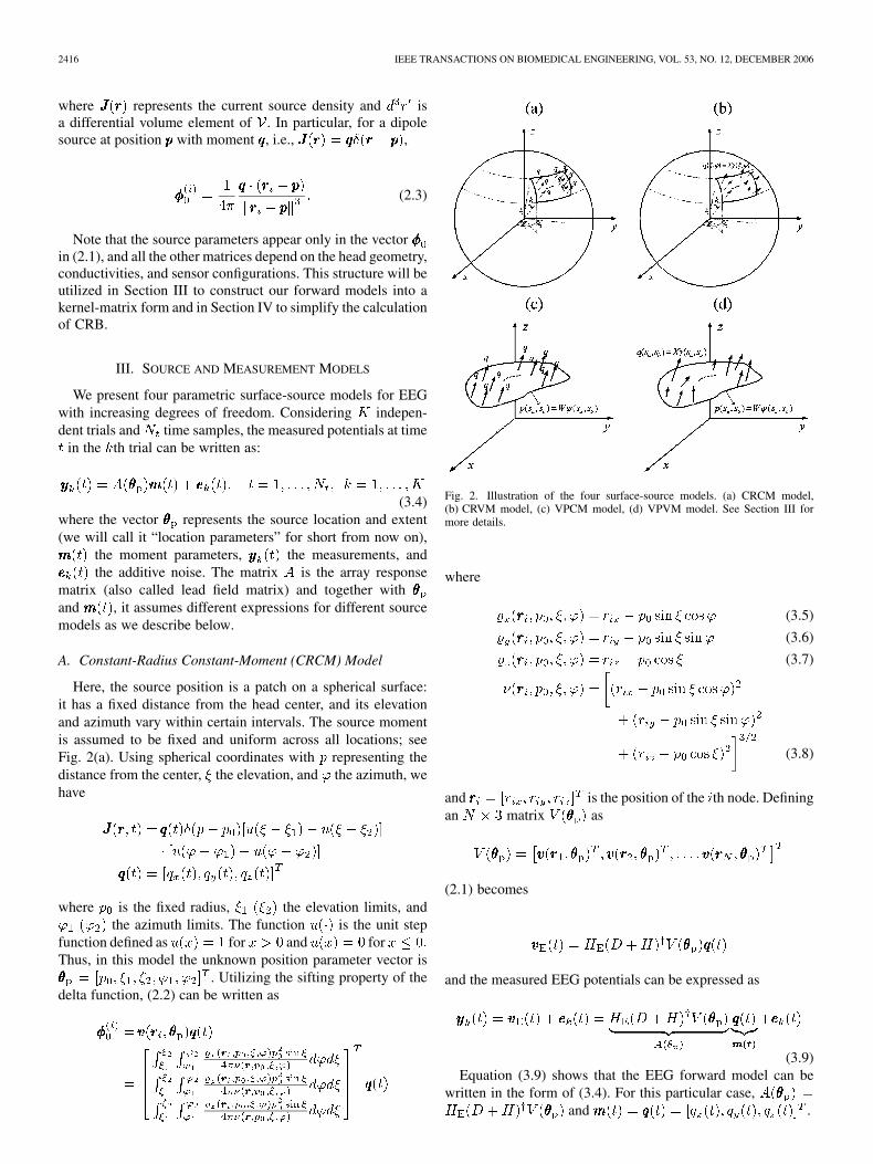
Here, the source position is a patch on a spherical surface:it has a fixed distance from the head center, and its elevationand azimuth vary within certain intervals. The source momentis assumed to be fixed and uniform across all locations; seeFig. 2(a). Using spherical coordinates with representing thedistance from the center, the elevation, and the azimuth, wehave

where is the fixed radius, the elevation limits, andthe azimuth limits. The function is the unit step

function defined as for and forThus, in this model the unknown position parameter vector is

. Utilizing the sifting property of thedelta function, (2.2) can be written as

Fig. 2. Illustration of the four surface-source models. (a) CRCM model,(b) CRVM model, (c) VPCM model, (d) VPVM model. See Section III formore details.

where

(3.5)

(3.6)

(3.7)

(3.8)

and is the position of the th node. Definingan matrix as

(2.1) becomes

and the measured EEG potentials can be expressed as

(3.9)Equation (3.9) shows that the EEG forward model can be

written in the form of (3.4). For this particular case,and .


B. Constant-Radius Variable-Moment (CRVM) Model

We allow the source moment density to change with its posi-tion in this model. Accordingly, the current density becomes

(3.10)

(3.11)

and the unknown position parameter vector remains the sameas in the CRCM model; see Fig. 2(b). We assume the spatialdistribution of the moment density can be describedby a linear combination of basis functions as

(3.12)

where is anvector of known basis functions, and is a matrix oftime varying unknown coefficients [4], [21]. This parameteri-zation allows us to exploit the prior information and reduce thenumber of unknown parameters. Substituting (3.10)–(3.12) into(2.2), we have

(3.13)

where ,, and the

th row of the th block is

The operator “ ” transforms a matrix into a column vectorby stacking its columns on top of each other, and the func-tions , , , and

are defined in (3.5)–(3.8).

C. Variable-Position Constant-Moment (VPCM) Model

This model provides more degrees of freedom for the sourceposition than the previous two models: the source position isallowed to be in an arbitrary shape in 3-D space instead of justa patch on a spherical surface; see Fig. 2(c). We represent thesource position in Cartesian coordinates as

(3.14)

where and are the surface parameters with limitsand . Accordingly, the source current density becomesas shown in (3.15) and (3.16) at the bottom of the page.

We describe the spatial variation of the source positionas

(3.17)

where isa vector of known basis functions, and is a matrixof unknown coefficients. Substituting (3.15)–(3.17) into (2.1)and (2.2), we have

(3.18)

where ,, and the th row of the matrix

is

with

(3.19)

(3.20)

(3.21)

(3.22)

(3.23)

elsewhere(3.15)

(3.16)


D. Variable-Position Variable-Moment (VPVM) Model

This is the most general model: the source position consistsof an arbitrary parametric shape and the source moment is al-lowed to vary along the position; see Fig. 2(d). Hence, the cur-rent density is as shown in (3.24) and (3.25) at the bottom of thepage. We model the source position using (3.17) anddescribe the spatial variation of the moment densityusing basis functions as

(3.26)

where isan vector of known basis functions, and is a ma-trix of time varying unknown coefficients. Substituting (3.17),(3.24) and (3.26) into (2.1) and (2.2), we have

(3.27)

where ,, and is an matrix:

The th row of the th submatrix is

where and the func-tions , , ,

, and are defined in (3.19)–(3.23).

E. Parameter Estimation

We use the ML method to estimate the source parametersand , based on the measurement model (3.4). The ML cri-terion is known to be asymptotically optimal in the sense that ithas the asymptotic properties of being unbiased, achieving theCRB (see Section IV,) and having a Gaussian probability den-sity function [24]. It has been applied to EEG/MEG source lo-calization and signal estimation in [4], [21], [37], [38], and wasshown in [38] to be more effective (than the principal compo-nent analysis after prestimulus based whitening) with nonsta-tionary noise. Assuming zero-mean Gaussian noise that is spa-tially and temporarily uncorrelated, the maximum-likelihoodestimate (MLE) of is [4], [21]

(3.28)

where

(3.29)

(3.30)and the MLE of is

(3.31)

Note that it is possible to consider more complex noise modelssuch as spatially correlated [4] or spatiotemporally correlated[37], [38] Gaussian noise, but we are not going to explore thisaspect in this paper since our main focus is on the surface-sourcemodeling.

IV. CRAMÉR-RAO BOUND

The CRB is a lower bound on the covariance of any unbiasedestimator. It is independent of the algorithm used for the esti-mation, and thus establishes a universal performance limit. It isan asymptotically tight bound under certain hypotheses; i.e., thebound can be achieved as the number of data samples becomesvery large. For a certain problem, if the ML estimator exists, itcan asymptotically achieve the CRB [24], [25].

Let represent all the unknown source parameters (e.g.,

for our models), be an unbiased

estimator of , and denote the Fisher information matrix(FIM). The Cramér-Rao inequality establishes that

(4.32)where the inequality sign states that the difference between thematrices on the left and right sides is positive semidefinite. Notethat the diagonal elements of the matrix are particularlyuseful since they set bounds on the variance of the parameters.

For the measurement model (3.4), assuming zero-meanGaussian noise with covariance matrix , the Fisherinformation matrix is

...

where

elsewhere(3.24)

(3.25)


the matrix is an identity matrix, “ ” denotes theKronecker product [39], and is defined as [4], [21]

(4.33)

Utilizing the structure of in (3.4), we rewrite as

(4.34)

where is the number of unknown position parameters andis an identity matrix. In this way, we need to calculateonly the second part of (4.34) for any possible , reducing thecomputational cost to obtain CRBs for a certain subject.

V. NUMERICAL EXAMPLES

We conducted a series of experiments to demonstrate the ap-plicability of proposed models in estimating the extended sur-face sources. We use both the simulated EEG data based on athree-layer RHM and electric measurements obtained from aphantom body. The RHM is composed of the brain, skull, andscalp, with the conductivity values being 0.33 for thescalp and brain and 0.0042 for the skull [23], [30],[40]. The inter-layer surfaces were tessellated into a total of9448 triangles (3074 on the brain, 3078 on the skull, and 3296 onthe scalp with a side length of 7.0 mm, 7.5 mm, and 8.0 mm, re-spectively) using the software Curry (Compumedics Neuroscan,El Paso, USA). This tessellation can provides us with accept-able errors from head modeling according to a previous studyby Haueisen et al. [41]. We used 32 electrodes distributed onthe scalp of a subject (see [42] for the detailed setup) and usedlinear discretization [23], [43]–[45] to calculate the , , and

in the forward models.

A. Numerical Results Using Simulated EEG Data

We first present results using the simulated EEG data.Throughout this subsection, we selected the noise varianceto obtain a signal-to-noise ratio (SNR) of 20 dB [40]. Wedefine SNR as , where

is the signal power at the th sensor.1) Comparison of Different Models: We assumed two types

of source distributions and estimated the source parametersusing the proposed surface-source models and dipole model.We used the mean-squared error to analyze the estimationaccuracy and choose the best-fitting model.

Example 1: We used a surface source with a fixed distancefrom the center , varying elevation with limits

and , and varying azimuth with limitsand . We chose the moment density to

be , , and, and applied the CRVM

model to generate the electric potentials.We estimated the source parameters using the proposed

models as well as the dipole model. For the CRVM model, weused basis functions , and for the

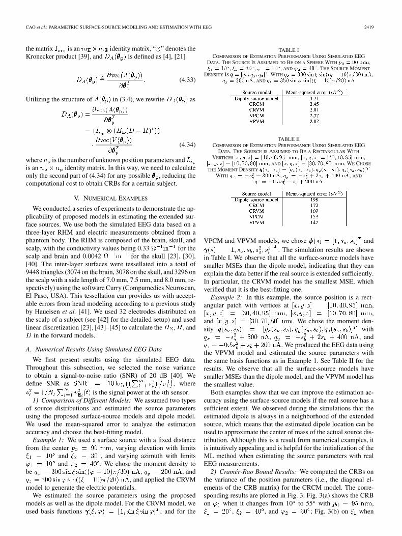
TABLE ICOMPARISON OF ESTIMATION PERFORMANCE USING SIMULATED EEG

DATA. THE SOURCE IS ASSUMED TO BE ON A SPHERE WITH p = 90 mm,� = 10 , � = 30 , ' = 10 , AND ' = 40 . THE SOURCE MOMENT

DENSITY IS qqq = [q ; q ; q ] WITH q = 300sin � sin(('� 10)�=30) nA,q = 300 nA, AND q = 350 sin' sin((� � 10)�=20) nA

TABLE IICOMPARISON OF ESTIMATION PERFORMANCE USING SIMULATED EEG

DATA. THE SOURCE IS ASSUMED TO BE A RECTANGULAR WITH

VERTICES [x; y; z] = [10;40;95] mm, [x; y; z] = [30;40;95] mm,[x; y; z] = [10;70;80] mm, AND [x; y; z] = [30;70;80] mm. WE CHOSE

THE MOMENT DENSITY qqq(s ; s ) = [q (s ; s ); q (s ; s ); q (s ; s )]WITH q = �s + 300 nA, q = �s + 2s + 400 nA, AND

q = �0:5s + s + 200 nA

VPCM and VPVM models, we chose and. The simulation results are shown

in Table I. We observe that all the surface-source models havesmaller MSEs than the dipole model, indicating that they canexplain the data better if the real source is extended sufficiently.In particular, the CRVM model has the smallest MSE, whichverified that it is the best-fitting one.

Example 2: In this example, the source position is a rect-angular patch with vertices at ,

, ,and . We chose the moment den-sity with

, , and. We produced the EEG data using

the VPVM model and estimated the source parameters withthe same basis functions as in Example 1. See Table II for theresults. We observe that all the surface-source models havesmaller MSEs than the dipole model, and the VPVM model hasthe smallest value.

Both examples show that we can improve the estimation ac-curacy using the surface-source models if the real source has asufficient extent. We observed during the simulations that theestimated dipole is always in a neighborhood of the extendedsource, which means that the estimated dipole location can beused to approximate the center of mass of the actual source dis-tribution. Although this is a result from numerical examples, itis intuitively appealing and is helpful for the initialization of theML method when estimating the source parameters with realEEG measurements.

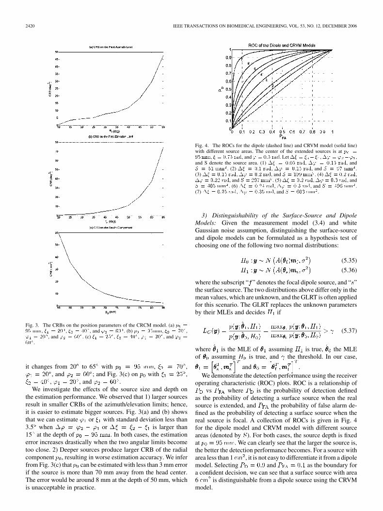
2) Cramér-Rao Bound Results: We computed the CRBs onthe variance of the position parameters (i.e., the diagonal el-ements of the CRB matrix) for the CRCM model. The corre-sponding results are plotted in Fig. 3. Fig. 3(a) shows the CRBon when it changes from 10 to 55 with ,

, , and ; Fig. 3(b) on when


Fig. 3. The CRBs on the position parameters of the CRCM model. (a) p =

95 mm, � = 20 , � = 40 , and ' = 60 . (b) p = 95mm, � = 70 ,' = 20 , and ' = 60 . (c) � = 25 , � = 40 , ' = 20 , and ' =

60 .

it changes from 20 to 65 with , ,, and ; and Fig. 3(c) on with ,

, , and .We investigate the effects of the source size and depth on

the estimation performance. We observed that 1) larger sourcesresult in smaller CRBs of the azimuth/elevation limits; hence,it is easier to estimate bigger sources. Fig. 3(a) and (b) showsthat we can estimate or with standard deviation less than3.5 when or is larger than15 at the depth of . In both cases, the estimationerror increases drastically when the two angular limits becometoo close. 2) Deeper sources produce larger CRB of the radialcomponent , resulting in worse estimation accuracy. We inferfrom Fig. 3(c) that can be estimated with less than 3 mm errorif the source is more than 70 mm away from the head center.The error would be around 8 mm at the depth of 50 mm, whichis unacceptable in practice.

Fig. 4. The ROCs for the dipole (dashed line) and CRVM model (solid line)with different source areas. The center of the extended sources is at p =

95mm, � = 0:75 rad, and ' = 0:5 rad. Let �� = � �� , �' = ' �' ,and S denote the source area. (1) �� = 0:05 rad, �' = 0:15 rad, andS = 51 mm . (2) �� = 0:1 rad, �' = 0:15 rad, and S = 97 mm .(3) �� = 0:15 rad, �' = 0:2 rad, and S = 199 mm . (4) �� = 0:2 rad,�' = 0:22 rad, and S = 297mm . (5) �� = 0:2 rad, �' = 0:3 rad, andS = 405 mm . (6) �� = 0:24 rad, �' = 0:3 rad, and S = 496 mm .(7) �� = 0:25 rad, �' = 0:35 rad, and S = 603 mm .

3) Distinguishability of the Surface-Source and DipoleModels: Given the measurement model (3.4) and whiteGaussian noise assumption, distinguishing the surface-sourceand dipole models can be formulated as a hypothesis test ofchoosing one of the following two normal distributions:

(5.35)

(5.36)

where the subscript “ ” denotes the focal dipole source, and “ ”the surface source. The two distributions above differ only in themean values, which are unknown, and the GLRT is often appliedfor this scenario. The GLRT replaces the unknown parametersby their MLEs and decides if

(5.37)

where is the MLE of assuming is true, the MLEof assuming is true, and the threshold. In our case,

and .We demonstrate the detection performance using the receiver

operating characteristic (ROC) plots. ROC is a relationship ofvs where is the probability of detection defined

as the probability of detecting a surface source when the realsource is extended, and the probability of false alarm de-fined as the probability of detecting a surface source when thereal source is focal. A collection of ROCs is given in Fig. 4for the dipole model and CRVM model with different sourceareas (denoted by ). For both cases, the source depth is fixedat . We can clearly see that the larger the source is,the better the detection performance becomes. For a source witharea less than 1 , it is not easy to differentiate it from a dipolemodel. Selecting and as the boundary fora confident decision, we can see that a surface source with area6 is distinguishable from a dipole source using the CRVMmodel.


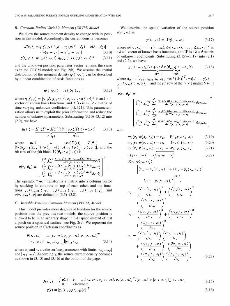
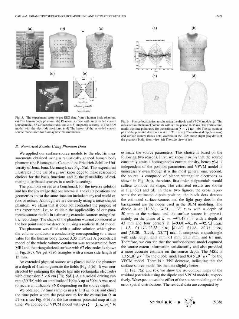
Fig. 5. The experiment setup to get EEG data from a human body phantom.(a) The human body phantom. (b) Phantom surface with an extended currentsource model, 67 surface electrodes, and 2� 31 magnetic sensors. (c) The BEMmodel with the electrode positions. (c,d) The layout of the extended currentsource model used for biomagnetic measurements.

B. Numerical Results Using Phantom Data

We applied our surface-source models to the electric mea-surements obtained using a realistically shaped human bodyphantom (the Biomagnetic Center of the Friedrich-Schiller-Uni-versity of Jena, Jena, Germany); see Fig. 5(a). This experimentillustrates 1) the use of a priori knowledge to make reasonablechoices for the basis functions and 2) the plausibility of esti-mating distributed sources in a realistic setting.

The phantom serves as a benchmark for the inverse solutionand has the advantage that one knows all the exact positions andgeometries and at the same time can include many real world er-rors or noises. Although we are currently using a torso-shapedphantom, we claim that it does not contradict the purpose ofthis experiment, i.e., to validate the applicability of our para-metric source models in estimating extended sources using elec-tric recordings. The shape of the phantom was not considered asthe key point since we describe it using a realistic BEM model.

The phantom was filled with a saline solution which givesthe volume conductor a conductivity corresponding to a meanvalue for the human body (about 3.35 mS/cm.) A geometricalmodel of the whole volume conductor was reconstructed fromMRI and the triangularized surface with 67 electrodes is shownin Fig. 5(c). We get 8796 triangles with a mean side length of15 mm.

An extended physical source was placed inside the phantomat a depth of 4 cm to generate the fields [Fig. 5(b)]. It was con-structed by enlarging the dipole tips into rectangular electrodeswith dimension 5 6 cm [Fig. 5(d)]. A sinusoidal driving cur-rent (30 Hz) with an amplitude of 100 uA up to 500 uA was usedto secure an utilizable SNR depending on the source depth.

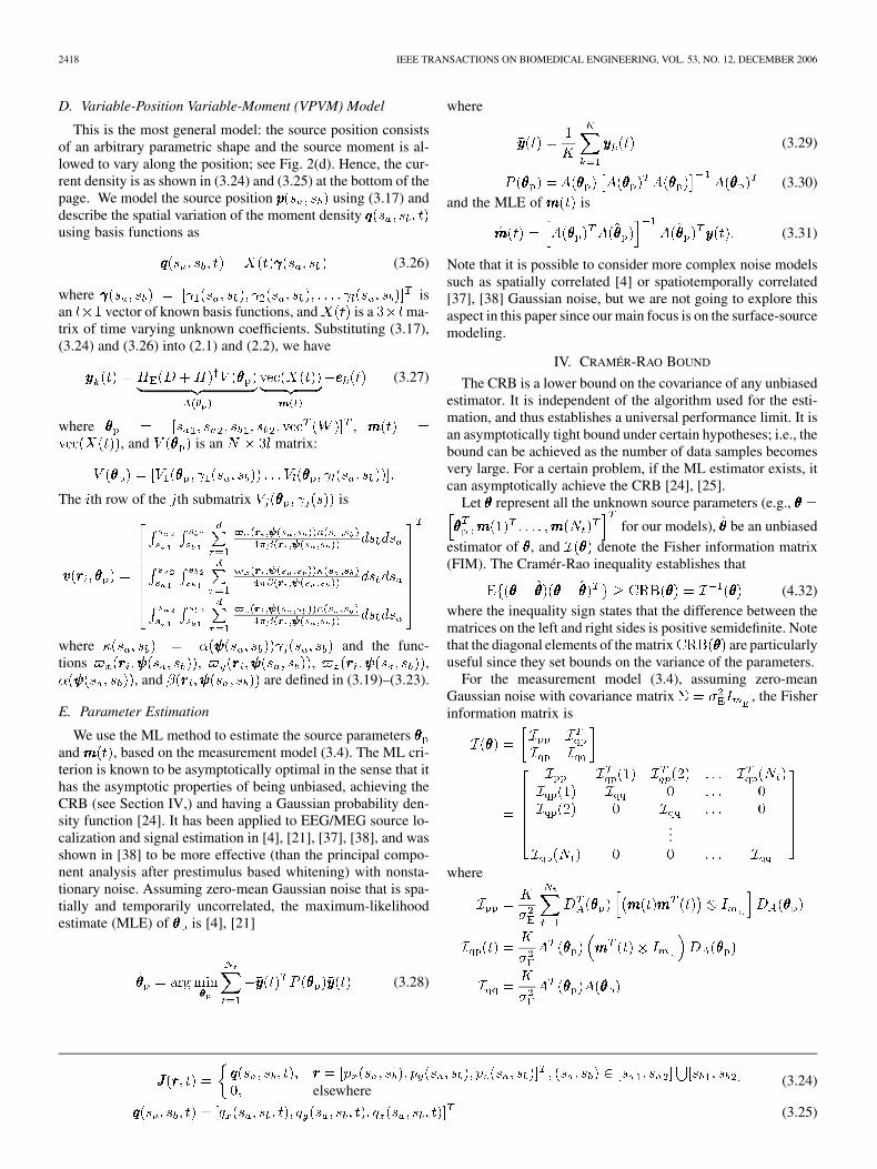
We obtained 39 time samples in a trial [Fig. 6(a)] and chosethe time point where the peak occurs for the estimation

; see Fig. 6(b) for the iso-contour potential map at thattime. We applied our VPCM model with to

Fig. 6. Source localization results using the dipole and VPCM models. (a) Themeasured multichannel potentials within time period 0–38 ms. The vertical linemarks the time point used for the estimation (t = 21 ms). (b) The iso-contourplot of the potential distribution at t = 21ms. (c) The estimated dipole (cross)and surface sources (black dots) overlaid in the BEM mesh (light gray dots) ofthe phantom body; front view. (d) The side view of (c).

estimate the source parameters. This choice is based on thefollowing two reasons. First, we know a priori that the sourceconstantly emits a homogeneous current density, hence isindependent of the position parameters and VPVM model isunnecessary even though it is the most general one. Second,the source is composed of planar rectangular electrodes asshown in Fig. 5(d), therefore. first-order polynomials wouldsuffice to model its shape. The estimated results are shownin Fig. 6(c) and (d). In these two figures, the cross repre-sents the estimated dipole position, the black dots denotesthe estimated surface source, and the light gray dots in thebackground are the nodes used in the BEM modeling. Thedipole is at with a depth of50 mm to the surface, and the surface source is approxi-mately on the plane of with a depth of43 mm and four corners at ,

, ,and . It composes a quadranglewith side length 55.3 mm, 61 mm, 53.5 mm, and 61 mm.Therefore, we can see that the surface-source model capturedthe source extent information satisfactorily and also provideda more accurate estimate on the source depth. The MSE is1.3 for the dipole model and 8.4 for theVPCM model. There is a 35% decrease, indicating that thesurface-source model fits the data slightly better.

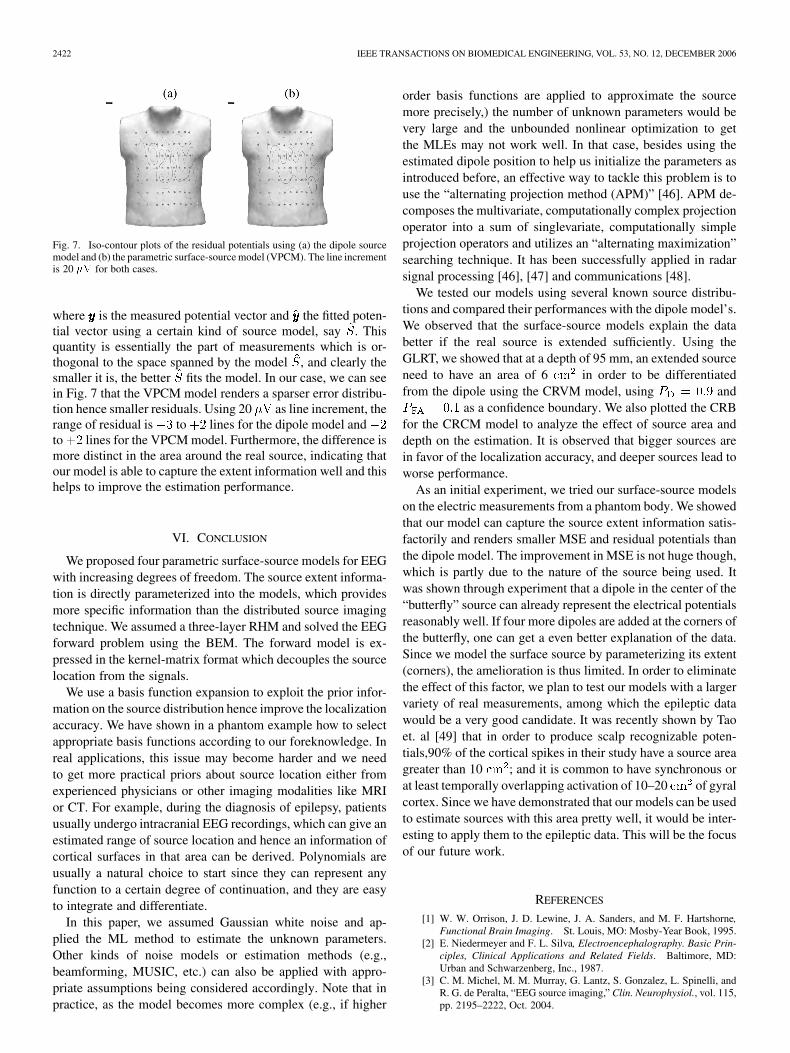
In Fig. 7(a) and (b), we show the iso-contour maps of theresidual potentials using the dipole and VPCM models, respec-tively. We expect to see the effect of the source modeling on theerror spatial distributions. The residual data are computed by

(5.38)


Fig. 7. Iso-contour plots of the residual potentials using (a) the dipole sourcemodel and (b) the parametric surface-source model (VPCM). The line incrementis 20 �V for both cases.

where is the measured potential vector and the fitted poten-tial vector using a certain kind of source model, say . Thisquantity is essentially the part of measurements which is or-thogonal to the space spanned by the model , and clearly thesmaller it is, the better fits the model. In our case, we can seein Fig. 7 that the VPCM model renders a sparser error distribu-tion hence smaller residuals. Using 20 as line increment, therange of residual is to lines for the dipole model andto lines for the VPCM model. Furthermore, the difference ismore distinct in the area around the real source, indicating thatour model is able to capture the extent information well and thishelps to improve the estimation performance.

VI. CONCLUSION

We proposed four parametric surface-source models for EEGwith increasing degrees of freedom. The source extent informa-tion is directly parameterized into the models, which providesmore specific information than the distributed source imagingtechnique. We assumed a three-layer RHM and solved the EEGforward problem using the BEM. The forward model is ex-pressed in the kernel-matrix format which decouples the sourcelocation from the signals.

We use a basis function expansion to exploit the prior infor-mation on the source distribution hence improve the localizationaccuracy. We have shown in a phantom example how to selectappropriate basis functions according to our foreknowledge. Inreal applications, this issue may become harder and we needto get more practical priors about source location either fromexperienced physicians or other imaging modalities like MRIor CT. For example, during the diagnosis of epilepsy, patientsusually undergo intracranial EEG recordings, which can give anestimated range of source location and hence an information ofcortical surfaces in that area can be derived. Polynomials areusually a natural choice to start since they can represent anyfunction to a certain degree of continuation, and they are easyto integrate and differentiate.

In this paper, we assumed Gaussian white noise and ap-plied the ML method to estimate the unknown parameters.Other kinds of noise models or estimation methods (e.g.,beamforming, MUSIC, etc.) can also be applied with appro-priate assumptions being considered accordingly. Note that inpractice, as the model becomes more complex (e.g., if higher

order basis functions are applied to approximate the sourcemore precisely,) the number of unknown parameters would bevery large and the unbounded nonlinear optimization to getthe MLEs may not work well. In that case, besides using theestimated dipole position to help us initialize the parameters asintroduced before, an effective way to tackle this problem is touse the “alternating projection method (APM)” [46]. APM de-composes the multivariate, computationally complex projectionoperator into a sum of singlevariate, computationally simpleprojection operators and utilizes an “alternating maximization”searching technique. It has been successfully applied in radarsignal processing [46], [47] and communications [48].

We tested our models using several known source distribu-tions and compared their performances with the dipole model’s.We observed that the surface-source models explain the databetter if the real source is extended sufficiently. Using theGLRT, we showed that at a depth of 95 mm, an extended sourceneed to have an area of 6 in order to be differentiatedfrom the dipole using the CRVM model, using and

as a confidence boundary. We also plotted the CRBfor the CRCM model to analyze the effect of source area anddepth on the estimation. It is observed that bigger sources arein favor of the localization accuracy, and deeper sources lead toworse performance.

As an initial experiment, we tried our surface-source modelson the electric measurements from a phantom body. We showedthat our model can capture the source extent information satis-factorily and renders smaller MSE and residual potentials thanthe dipole model. The improvement in MSE is not huge though,which is partly due to the nature of the source being used. Itwas shown through experiment that a dipole in the center of the“butterfly” source can already represent the electrical potentialsreasonably well. If four more dipoles are added at the corners ofthe butterfly, one can get a even better explanation of the data.Since we model the surface source by parameterizing its extent(corners), the amelioration is thus limited. In order to eliminatethe effect of this factor, we plan to test our models with a largervariety of real measurements, among which the epileptic datawould be a very good candidate. It was recently shown by Taoet. al [49] that in order to produce scalp recognizable poten-tials,90% of the cortical spikes in their study have a source areagreater than 10 ; and it is common to have synchronous orat least temporally overlapping activation of 10–20 of gyralcortex. Since we have demonstrated that our models can be usedto estimate sources with this area pretty well, it would be inter-esting to apply them to the epileptic data. This will be the focusof our future work.

REFERENCES

[1] W. W. Orrison, J. D. Lewine, J. A. Sanders, and M. F. Hartshorne,Functional Brain Imaging. St. Louis, MO: Mosby-Year Book, 1995.

[2] E. Niedermeyer and F. L. Silva, Electroencephalography. Basic Prin-ciples, Clinical Applications and Related Fields. Baltimore, MD:Urban and Schwarzenberg, Inc., 1987.

[3] C. M. Michel, M. M. Murray, G. Lantz, S. Gonzalez, L. Spinelli, andR. G. de Peralta, “EEG source imaging,” Clin. Neurophysiol., vol. 115,pp. 2195–2222, Oct. 2004.


[4] A. Dogandzic and A. Nehorai, “Estimating evoked dipole responsesin unknown spatially correlated noise with EEG/MEG arrays,” IEEETrans. Signal Process., vol. 48, no. 1, pp. 13–25, Jan. 2000.

[5] J. C. Mosher, R. M. Leahy, and P. S. Lewis, “EEG and MEG: Forwardsolutions for inverse methods,” IEEE Trans. Biomed. Eng., vol. 46, no.3, pp. 245–259, Mar. 1999.

[6] G. Nolte and G. Curio, “Current multipole expansion to estimate lat-eral extent of neuronal activity: A theoretical analysis,” IEEE Trans.Biomed. Eng., vol. 47, no. 10, pp. 1347–1355, Oct. 2000.

[7] K. Jerbi, J. Mosher, G. Nolte, S. Baillet, L. Garnero, and R. Leahy,“From dipoles to multipoles: Parametric solutions to the inverseproblem in MEG,” presented at the 13th Int. Conf. Biomagnetism,Jena, Germany, Aug. 2002.

[8] B. Lütkenhöner, E. Menninghaus, O. Steinsträter, C. Wienbruch, H. M.Gissler, and T. Elbert, “Neuromagnetic source analysis using magneticresonance images for the construction of source and volume conductormodel,” Brain Topogr., vol. 7, pp. 291–299, 1995.

[9] W. E. Kincses, C. Braun, S. Kaiser, and T. Elbert, “Modeling extendedsources of event-related potentials using anatomical and physiologicalconstraints,” Hum. Brain Mapp., vol. 8, pp. 182–193, Apr. 1999.

[10] T. Limpiti, A. Bolstad, B. D. van Veen, and R. T. Wakai, “Detectionof cortical patch activity in beamspace using the generalized likelihoodratio test,” in Proc. 5th Int. Conf. BME and NFSI, Minneapolis, MN,May 2005, pp. 26–29.

[11] M. Wagner, T. Kohler, M. Fuchs, and J. Kastner, R. I. J. Nenonen and T.Katila, Eds., “An extended source model for current density reconstruc-tions,” in Proc. 12th Int. Conf. Biomagnetism, Espoo, Finland, Aug.2000, pp. 749–752.

[12] L. Gavit, S. Baillet, J. Mangin, J. Pescatore, and L. Garnero, “A mul-tiresolution framework to MEG/EEG source imaging,” IEEE Trans.Biomed. Eng., vol. 48, no. 10, pp. 1080–1087, Oct. 2001.

[13] R. D. Pascula-Marqui, C. M. Michel, and D. Lehmann, “Low resolutionelectromagnetic tomography: A new method for localizing electricalactivity of the brain,” Int. J. Phychophysiol., vol. 18, pp. 49–65, Oct.1994.

[14] J. Sarvas, “Basic mathematical and electromagnetic concepts of bio-magnetic inverse problem,” Phys. Med. Biol., vol. 32, pp. 11–22, Jan.1987.

[15] I. Gorodnistky, J. George, and B. Rao, “Neuromagnetic sourceimaging with focuss: A recursive weighted minimum-norm al-gorithm,” Electroencephalogr. Clin. Neurophysiol., vol. 95, pp.231–251, Oct. 1995.

[16] P. Valdes-Sosa, F. Marti, F. Gaicia, and R. Casanova, “Variable reso-lution electric-magnetic tomography,” presented at the 10th Int. Conf.Biomagnetism, New York, 2000.

[17] M. Fuchs, M. Wagner, T. Kohler, and H. -A. Wischmann, “Linear andnonlinear current density reconstructions,” J. Clin. Neurophysiol., vol.16, pp. 267–295, May 1999.

[18] B. He, X. Zhang, J. Lian, H. Sasaki, D. Wu, and V. L. Towle,“Boundary element method-based cortical potential imaging of so-matosensory evoked potentials using subjects’ magnetic resonanceimaging,” NeuroImage, vol. 16, pp. 564–576, 2002.

[19] X. Zhang, W. van Drongelen, K. Hecox, V. Towle, D. Frim, A. McGee,J. Lian, and B. He, “Localization of epileptic foci by means of corticalimaging using a spherical head model,” NeuroComputing, vol. 52–54,pp. 977–982, 2003.

[20] X. Zhang, W. van Drongelen, K. Hecox, V. Towle, D. Frim, A. McGee,and B. He, “High resolution EEG: Cortical imaging of interictal epilep-tiform spikes,” Clin. Neurophysiol., vol. 114, pp. 1963–1973, 2003.

[21] I. S. Yetik, A. Nehorai, C. Muravchik, and J. Haueisen, “Line-sourcemodeling and estimation with magnetoencephalography,” IEEE Trans.Biomed. Eng., vol. 52, no. 5, pp. 839–851, May 2005.

[22] N. Cao, S. I. Yetik, A. Nehorai, C. Muravchik, and J. Haueisen,“Line-source modeling and estimation with electroencephalography,”in Proc. 5th Int. Conf. BEM and NFSI, Minneapolis, MN, May 2005,pp. 82–85.

[23] J. C. Mosher, R. M. Leahy, and P. S. Lewis, “Matrix kernels for MEGand EEG source localization and imaging,” in Proc. IEEE Int. Conf.Acoustics, Speech, and Signal Processing, ICASSP 95, Detroit, MI,May 1995, vol. 5, pp. 2943–2946.

[24] S. M. Kay, Fundamentals of Statistical Signal Processing: EstimationTheory. Upper Saddle River, NJ: PTR Prentice Hal, 1993.

[25] H. L. Van Trees, Detection, Estimation and Modulation Theory. NewYork: Wiley, 1968.

[26] F. N. Wilson and R. H. Bailey, “The electrical field of an eccentricdipole in a homogeneous spherical conducting medium,” Circulation,vol. 1, pp. 84–92, 1950.

[27] J. C. De Munck and M. J. Peters, “A fast method to compute the po-tential in the multisphere model,” IEEE Trans. Biomed. Eng., vol. 40,no. 11, pp. 1166–1174, Nov. 1993.

[28] Z. Zhang, “A fast method to compute surface potentials generated bydipoles within multilayer anisotropic spheres,” Phys. Med. Biol., vol.40, pp. 335–349, Mar. 1995.

[29] B. N. Cuffin, “EEG localization accuracy improvements using realisti-cally shaped head models,” IEEE Trans. Biomed. Eng., vol. 43, no. 3,pp. 299–303, Mar. 1996.

[30] C. Muravchik and A. Nehorai, “EEG/MEG error bounds for a staticdipole source with a realistic head model,” IEEE Trans. SignalProcess., vol. 49, no. 3, pp. 470–484, Mar. 2001.

[31] B. N. Cuffin, “Effect of head shape on EEG’s and MEG’s,” IEEE Trans.Biomed. Eng., vol. 37, no. 1, pp. 44–52, Jan. 1990.

[32] ——, “A method for localizing EEG sources in realistic head models,”IEEE Trans. Biomed. Eng., vol. 42, no. 1, pp. 68–71, Jan. 1995.

[33] C. A. Brebbia and J. Dominguez, Boundary Elements. An IntroductoryCourse, 2nd ed. New York: McGraw-Hill.

[34] A. A. Becker, An Introductory Guide to Finite Element Analysis. NewYork: ASME, 2004.

[35] B. Vanrumste, G. Van Hoey, R. Van de Walle, M. R. D’Havè, I. A.Lemahieu, and P. A. Boon, “The validation of the finite differecemethod and reciprocity for solving the inverse problem in EEG dipolesource analysis,” Brain Topogr., vol. 14, no. 2, pp. 83–92, Dec. 2001.

[36] F. Darvas, D. Pantazis, E. Kucukaltun-Yildirim, and R. M. Leahy,“Mapping human brain function with meg and eeg: Methods andvalidation,” NeuroImage, vol. 23, pp. S289–S299, 2004.

[37] F. Bijma, J. C. de Munck, H. M. Huizenga, R. M. Heethaar, and A.Nehorai, “Simultaneous estimation and testing of sources in multipleMEG data sets,” IEEE Trans. Signal Process., vol. 53, no. 1, pp. 11–33,Jan. 2005.

[38] B. Baryshnikov, B. van Veen, and R. Wakai, “Maximum-likelihood es-timation of low-rank signals for multiepoch meg/eeg analysis,” IEEETrans. Biomed. Eng., vol. BME-51, no. 11, pp. 1981–1993, Nov. 2004.

[39] J. W. Brewer, “Kronecker products and matrix calculus in systemtheory,” IEEE Trans. Circuits Syst., vol. CAS-25, no. 9, pp. 772–781,Sep. 1978.

[40] D. Gutierrez, A. Nehorai, and C. Muravchik, “Estimating brain con-ductivities and dipole source signals with EEG arrays,” IEEE Trans.Biomed. Eng., vol. 51, no. 12, pp. 2113–2122, Dec. 2004.

[41] J. Haueisen, A. Boettner, M. Funke, H. Brauer, and H. Nowak, “Theinfluence of boundary element discretization on the forward and inverproblem in electroencephalography and magnetoencephalography,”Biomedizinische Technik, vol. 42, pp. 240–248, 1997.

[42] H. Buchner, M. Fuchs, H. A. Wischmann, O. Dössel, I. Ludwig, A.Knepper, and P. Berg, “Source analysis of median nerve and fingerstimulated somatosensory evoked potentials: Multichannel simulta-neous recording of electric and magnetic fields combined with 3D-MRtomography,” Brain Topogr., vol. 6, no. 4, pp. 299–310, 1994.

[43] J. C. de Munck, P. C. M. Vijn, and F. H. L. da Silva, “A random dipolemodel for spontaneous brain activity,” IEEE Trans. Biomed. Eng., vol.39, no. 8, pp. 791–804, Aug. 1992.

[44] A. S. Ferguson, X. Zhang, and G. Stroink, “A complete linear dis-cretization for calculating the magnetic field using the boundary ele-ment method,” IEEE Trans. Biomed. Eng., vol. 41, no. 5, pp. 455–460,May 1994.

[45] H. A. Schlitt, L. Heller, R. Aaron, E. Best, and D. M. Ranken, “Eval-uation of boundary element methods for the EEG forward problem:Effect of linear interpolation,” IEEE Trans. Biomed. Eng., vol. 42, no.1, pp. 52–58, Jan. 1995.

[46] I. Ziskind and M. Wax, “Maximum likelihood localization of multiplesources by alternating projection,” IEEE Trans. Signal Process., vol.36, no. 10, pp. 1553–1560, Oct. 1988.

[47] J. C. Chen, R. E. Hudson, and K. Yao, “Maximum-likelihood sourcelocalization and unknown sensor location estimation for wideband sig-nals in the near-field,” IEEE Trans. Signal Process., vol. 50, no. 8, pp.1843–1854, Aug. 2002.

[48] E. Ertin, U. Mitra, and S. Siwamogsatham, “Maximum-likeli-hood-based multipath channel estimation for code-division mul-tiple-access systems,” IEEE Trans. Commun., vol. 49, no. 2, pp.290–302, Feb. 2001.


[49] J. X. Tao, A. Ray, S. Hawes-Ebersole, and J. S. Ebersole, “IntracranialEEG substrates of scalp EEG interictal spikes,” Epilepsia, vol. 46, pp.669–676, May 2005.

Nannan Cao (S’06) received the B.S. degree in elec-trical engineering from the University of Science andTechnology of China, Hefei, in 2002. She is currentlyworking toward the Ph.D. degree in the Departmentof Electrical and Systems Engineering, WashingtonUniversity, St. Louis, MO.

Her research interest is in statistical signal pro-cessing with applications to biomedicine.

Imam Samil Yetik (M’05) was born in Istanbul,Turkey, in 1978. He received the B.Sc. degree inelectrical and electronics engineering from BogaziciUniversity, Istanbul, in 1998, the M.S. degree inelectrical and electronics engineering from BilkentUniversity, Ankara, Turkey, in 2000, and the Ph.D.degree in electrical and computer engineering fromthe University of Illinois at Chicago, in 2004.

He joined the Department of Electrical andComputer Engineering at the Illinois Institute ofTechnology as an Assistant Professor after his

postdoc positions at the University of Illinois at Chicago and University ofCalifornia at Davis. His research interests are in the areas of biomedical signaland image processing with emphasis on PET image reconstruction, imageregistration, and EEG/MEG.

Arye Nehorai (S’80–M’83–SM’90–F’94) receivedthe B.Sc. and M.Sc. degrees in electrical engineeringfrom the Technion, Haifa, Israel, and the Ph.D. de-gree in electrical engineering from Stanford Univer-sity, Stanford, CA.

From 1985 to 1995, he was a faculty member withthe Department of Electrical Engineering at YaleUniversity, New Haven, CT. In 1995, he joined theDepartment of Electrical Engineering and ComputerScience at The University of Illinois at Chicago(UIC) as Full Professor. From 2000 to 2001, he

was Chair of the department’s Electrical and Computer Engineering (ECE)Division, which then became a new department. In 2001, he was namedUniversity Scholar of the University of Illinois. In 2006, he assumed theChairman position of the Department of Electrical and Systems Engineering atWashington University, St. Louis, MO, where he is also the inaugural holder ofthe Eugene and Martha Lohman Professorship of Electrical Engineering. He

is the Principal Investigator of the new multidisciplinary university researchinitiative (MURI) project entitled Adaptive Waveform Diversity for FullSpectral Dominance.

Dr. Nehorai was Editor-in-Chief of the IEEE TRANSACTIONS ON SIGNAL

PROCESSING during the years 2000 to 2002. In 2003–2005, he was VicePresident (Publications) of the IEEE Signal Processing Society, Chair of thePublications Board, member of the Board of Governors, and member of theExecutive Committee of this Society. He is the founding editor of the specialcolumns on Leadership Reflections in the IEEE Signal Processing Magazine.He was co-recipient of the IEEE SPS 1989 Senior Award for Best Paperwith P. Stoica, co-author of the 2003 Young Author Best Paper Award andco-recipient of the 2004 Magazine Paper Award with A. Dogandzic. He waselected Distinguished Lecturer of the IEEE SPS for the term 2004 to 2005. Hehas been a Fellow of the Royal Statistical Society since 1996.

Carlos H. Muravchik (S’81–M’83–SM’99) wasborn in Argentina, June 11, 1951. He graduated as anElectronics Engineer from the National University ofLa Plata, La Plata, Argentina, in 1973. He receivedthe M.Sc. in statistics (1983) and the M.Sc. (1980)and Ph.D. (1983) degrees in electrical engineering,from Stanford University, Stanford, CA.

He is a Professor at the Department of the Elec-trical Engineering of the National University of LaPlata and a member of its Industrial Electronics, Con-trol and Instrumentation Laboratory (LEICI). He is

also a member of the Comision de Investigaciones Cientificas de la Pcia. deBuenos Aires. He was a Visiting Professor at Yale University in 1983 and 1994,and at the University of Illinois at Chicago in 1996, 1997, 1999, and 2003. Since1999, he is a member of the Advisory Board of the journal Latin American Ap-plied Research. His research interests are in the area of statistical signal andarray processing with biomedical, control and communications applications,and nonlinear control systems.

Dr. Muravchik was an Associate Editor of the IEEE TRANSACTIONS ON

SIGNAL PROCESSING (2003–2006).

Jens Haueisen (M’02) received the M.S. and Ph.D.degrees in electrical engineering from the TechnicalUniversity Ilmenau, Ilmenau, Germany, in 1992 and1996, respectively.

From 1996 to 1998 he worked as a Post-Doc andfrom 1998 to 2005 as the head of the BiomagneticCenter, Friedrich-Schiller-University, Jena, Ger-many. Since 2005, he is Professor of BiomedicalEngineering and directs the Institute of Biomed-ical Engineering and Informatics at the TechnicalUniversity Ilmenau. His research interests are in

the numerical computation of bioelectromagnetic fields and the analysis ofbioelectromagnetic signals.

2414 ieee transactions on biomedical engineering, … · parametric surface-source modeling and...

Documents