Chapter 25Field Plots andElectric Potential

THE CONTOUR MAPFigure (1) is a contour map of a small island. Thecontour lines, labeled 0, 10, 20, 30 and 40 are lines ofequal height. Anywhere along the line marked 10 theland is 10 meters above sea level. (You have to look atsome note on the map that tells you that height ismeasured in meters, rather than feet or yards.)

You can get a reasonable understanding of the terrainjust by looking at the contour lines. On the south sideof the island where the contour lines are far apart, theland slopes gradually upward. This is probably wherethe beach is located. On the north side where thecontour lines are close together, the land drops offsharply. We would expect to see a cliff on this side ofthe island.

Figure 1Contour map of a small island with a beach on thesouth shore, two hills, and a cliff on the northwestside. The slope of the island is gradual where thelines are far apart, and steep where the lines areclose together. If you were standing at the pointlabeled (A) and the surface were slippery, youwould start to slide in the direction of the arrow.

sea level

10

20

0

30 30

N

A

40 40

CHAPTER 25 FIELD PLOTS AND ELEC-TRIC POTENTIAL

Calculating the electric field of any but the simplestdistribution of charges can be a challenging task.Gauss’ law works well where there is considerablesymmetry, as in the case of spheres or infinite lines ofcharge. At the beginning of Chapter (24), we were ableto use a brute force calculus calculation to determinethe electric field of a short charged rod. But to handlemore complex charge distributions we will find ithelpful to apply the techniques developed by mapmakers to describe complex terrains on a flat map. Thisis the technique of the contour map which worksequally well for mapping electric fields and mountainranges. Using the contour map ideas, we will be leadto the concept of a potential and equipotential lines orsurfaces, which is the main topic of this chapter.

25-2 Field Plots and Electric Potential

Although we would rather picture this island as beingin the south seas, imagine that it is in the North Atlanticand a storm has just covered it with a sheet of ice. Youare standing at the point labeled A in Figure (1), andstart to slip. If the surface is smooth, which way wouldyou start to slip?

A contour line runs through Point A which we haveshown in an enlargement in Figure (2). You would notstart to slide along the contour line because all thepoints along the contour line are at the same height.Instead, you would start to slide in the steepest down-hill direction, which is perpendicular to the contour lineas shown by the arrow.

If you do not believe that the direction of steepestdescent is perpendicular to the contour line, choose anysmooth surface like the top of a rock, mark a horizontalline (an equal height line) for a contour line, andcarefully look for the directions that are most steeplysloped down. You will see that all along the contourline the steepest slope is, in fact, perpendicular to thecontour line.

Skiers are familiar with this concept. When you wantto stop and rest and the slope is icy, you plant your skisalong a contour line so that they will not slide eitherforward or backward. The direction of steepest descentis now perpendicular to your skis, in a direction that skiinstructors call the fall line. The fall line is the directionyou will start to slide if the edges of your skis fail tohold.

In Figure (3), we have redrawn our contour map of theisland, but have added a set of perpendicular lines toshow the directions of steepest descent, the direction ofthe net force on you if you were sitting on a slipperysurface. These lines of steepest descent, are also calledlines of force. They can be sketched by hand, using therule that the lines of force must always be perpendicularto the contour lines.

A

Figure 3You can sketch in the lines of steepest descentby drawing a set of lines that are alwaysperpendicular to the contour lines. Theselines indicate the direction a ball would startto roll if placed at a point on the line.

Acontour lines

direction of steepestdescent

Figure 2Along a contour line the land is level. Thedirection of steepest slope or descent isperpendicular to the contour line.

25-3

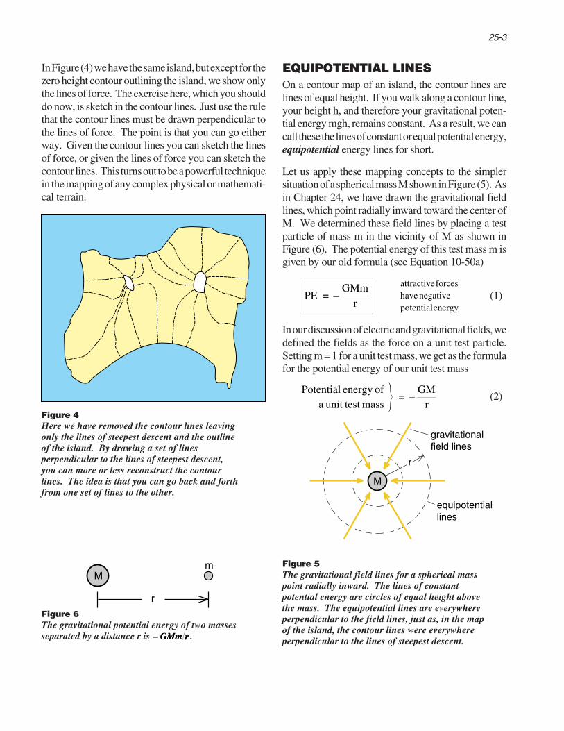
In Figure (4) we have the same island, but except for thezero height contour outlining the island, we show onlythe lines of force. The exercise here, which you shoulddo now, is sketch in the contour lines. Just use the rulethat the contour lines must be drawn perpendicular tothe lines of force. The point is that you can go eitherway. Given the contour lines you can sketch the linesof force, or given the lines of force you can sketch thecontour lines. This turns out to be a powerful techniquein the mapping of any complex physical or mathemati-cal terrain.

EQUIPOTENTIAL LINESOn a contour map of an island, the contour lines arelines of equal height. If you walk along a contour line,your height h, and therefore your gravitational poten-tial energy mgh, remains constant. As a result, we cancall these the lines of constant or equal potential energy,equipotential energy lines for short.

Let us apply these mapping concepts to the simplersituation of a spherical mass M shown in Figure (5). Asin Chapter 24, we have drawn the gravitational fieldlines, which point radially inward toward the center ofM. We determined these field lines by placing a testparticle of mass m in the vicinity of M as shown inFigure (6). The potential energy of this test mass m isgiven by our old formula (see Equation 10-50a)

PE = –

GMmr

attractiveforceshave negativepotentialenergy

(1)

In our discussion of electric and gravitational fields, wedefined the fields as the force on a unit test particle.Setting m = 1 for a unit test mass, we get as the formulafor the potential energy of our unit test mass

Potential energy ofa unit test mass

= –GM

r(2)

Figure 5The gravitational field lines for a spherical masspoint radially inward. The lines of constantpotential energy are circles of equal height abovethe mass. The equipotential lines are everywhereperpendicular to the field lines, just as, in the mapof the island, the contour lines were everywhereperpendicular to the lines of steepest descent.

M

r

equipotentiallines

gravitationalfield lines

Figure 4Here we have removed the contour lines leavingonly the lines of steepest descent and the outlineof the island. By drawing a set of linesperpendicular to the lines of steepest descent,you can more or less reconstruct the contourlines. The idea is that you can go back and forthfrom one set of lines to the other.

Figure 6The gravitational potential energy of two massesseparated by a distance r is – GMm rGMm r .

Mm

r

25-4 Field Plots and Electric Potential

From Equation (2) we see that if we stay a constantdistance r out from M, if we are one of the concentriccircles in Figure (5), then the potential energy of theunit test mass remains constant. These circles, drawnperpendicular to the lines of force, are again equalpotential energy lines.

There is a convention in physics to use the wordpotential when talking about the potential energy of aunit mass or unit charge. With this convention, then

– GM/r in Equation (2) is the formula for the gravita-tional potential of a mass M, and the constant radiuscircles in Figure (5) are lines of constant potential.Thus the name equipotential lines for these circles isfitting.

Negative and PositivePotential EnergyIn Figure (7) we have drawn the electric field lines ofa point charge Q and drawn the set of concentric circlesperpendicular to the field lines as shown. From theclose analogy between the electric and gravitationalforce, we expect that these circles represent lines ofconstant electric potential energy, that they are theelectric equipotential lines.

But there is one important difference between Figures(5) and (7). In Figure (5) the gravitational force on ourunit test mass is attractive, in toward the mass M. InFigure (7), the force on our unit positive test particle isout, away from Q if Q is positive. When we have anattractive force as in Figure (5), the potential energyis negative as in Equation (1). But when the force isrepulsive, as in Figure (7), the potential energy ispositive. Let us briefly review the physical origin forthis difference in the sign of the potential energy.

In any discussion of potential energy, it is necessary todefine the zero of potential energy, i.e. to say where thefloor is. In the case of satellite motion, we defined thesatellite’s potential energy as being zero when thesatellite was infinitely far away from the planet. If werelease a satellite at rest a great distance from the planet,it will start falling toward the planet. As it falls, it gainskinetic energy, which it must get at the expense ofgravitational potential energy. Since the satellite startedwith zero gravitational potential energy when far outand loses potential energy as it falls in, it must end upwith negative potential energy when it is near theplanet. This is the physical origin of the minus sign inEquation (1). Using the convention that potentialenergy is zero at infinity, then attractive forces lead tonegative potential energies.

If the force is repulsive as in Figure (7), then we haveto do work on our test particle in order to bring it in frominfinity. The work we do against the repulsive force isstored up as positive potential energy which could bereleased if we let go of the test particle (and the testparticle goes flying out). Thus the convention thatpotential energy is zero at infinity leads to positivepotential energies for repulsive forces like that shownin Figure (7).

+Q

r

equipotentiallines

electricfield lines

Figure 7The electric potential is the potential energy of apositive unit test charge qtest = + 1 coulomb.Because a positive charge + Q and a positive testcharge repel this potential energy is positive.

25-5

ELECTRIC POTENTIALOF A POINT CHARGEUsing the fact that we can go from the gravitationalforce law to Coulomb’s law by replacing GMm by

Qq 4πε0Qq 4πε0 (see Exercise 1), we expect that the formulafor the electric potential energy of a charge q a distancer from Q is

electric potential energyof a charge q

= +Qq

4πε0r(3)

The + sign in Equation (3) indicates that for positive Qand q we have a repulsive force and positive potentialenergy. (If Q is negative, but q still positive, the forceis attractive and the potential energy must be negative.)

To determine the potential energy of a unit test charge,we set q = 1 in Equation (3) to get

electric potentialenergy of a unittest charge

≡ electricpotential

=Qq

4πε0r

(4)

Following the same convention we used for gravity, wewill use the name electric potential for the potentialenergy of a unit test charge. Thus Equation (4) is theformula for the electric potential in the region sur-rounding the charge Q. As expected, the lines of equalpotential, the equipotential lines are the circles ofconstant radius seen in Figure (7).

Exercise 1

Start with Newton's gravitational force law, replaceGMm by Qq 4π ε0Qq 4π ε0 , and show that you end up withCoulomb's electrical force law.

CONSERVATIVE FORCES(This is a formal aside to introduce a point that we willtreat in much more detail later.)

Suppose we have a fixed charge Q and a small testparticle q as shown in Figure (8). The potential energyof q is defined as zero when it is infinitely far away fromQ. If we carry q in from infinity to a distance r, we doan amount of work on the particle

Work we do = Fus

∞

r

⋅dx (5)

If we apply just enough force to overcome the electricrepulsive force, if Fus = –qE , then the work we doshould all be stored as electric potential energy, andEquation (5), with Fus = –qE should give us thecorrect electric potential energy of the charge q.

But an interesting question arises. Suppose we bringthe charge q in along two different paths, paths (1) and(2) shown in Figure (8). Do we do the same amount ofwork, store the same potential energy for the twodifferent paths?

Figure 8If we bring a test particle q in from infinity toa distance r from the charge Q, the electricpotential energy equals Qq/4ππεεor . But thispotential energy is the work we do in bringingq in from infinity:

Fus ⋅⋅ dr

∞∞

r

=Qq

4ππεεor

This answer does not depend upon the path wetake bringing q in.

rQ Fusq Fe

dr

qFus

Fedr

path 1

path 2

25-6 Field Plots and Electric Potential

If we lift an eraser off the floor up to a height h, andhold it still, then it does not matter what path we took,the net amount of work we did was mgh and this isstored as gravitational potential energy. When thework we do against a force depends only on the initialand final points, and not on the path we take, we say thatthe force is conservative.

In contrast, if we move the eraser over a horizontal tablefrom one point to another, the amount of work we doagainst friction depends very much on the path. Thelonger the path the more work we do. As a result wecannot define a friction potential energy because ithas no unique value. Friction is a non-conservativeforce, and non-conservative forces do not have uniquepotential energies.

The gravitational fields of stationary masses and theelectric fields of stationary charges all produce conser-vative forces, and therefore have unique potentialenergies. We will see however that moving chargescan produce electric fields that are not conservative!When that happens, we will have to take a very carefullook at our picture of electric potential energy. But indealing with the electric fields of static charges, as wewill for a few chapters, we will have unique electricpotential energies, and maps of equipotential lines willhave an unambiguous meaning.

ELECTRIC VOLTAGEIn our discussion of Bernoulli’s equation, we gave thecollection of terms (P + ρgh + 1/2ρv2) the name hy-drodynamic voltage. The content of Bernoulli’s equa-tion is that this hydrodynamic voltage is constant alonga stream line when the fluid is incompressible andviscous forces can be neglected. Two of the threeterms, ρgh and 1/2ρv2 represent the energy of a unitvolume of the fluid, thus we see that our hydrodynamicvoltage has the dimensions of energy per unit volume.

Electric voltage is a quantity with the dimensions ofenergy per unit charge that in different situations isrepresented by a series of terms like the terms inBernoulli’s hydrodynamic voltage. There is the poten-tial energy of an electric field, the chemical energysupplied by a battery, even a kinetic energy term, seenin careful studies of superconductors, that is strictlyanalogous to the 1 21 2ρv2 term in Bernoulli’s equation.In other words, electric voltage is a complex concept,but it has one simplifying feature. Electric voltages aremeasured by a common experimental device called avoltmeter. In fact we will take as the definition ofelectric voltage, that quantity which we measure usinga voltmeter.

This sounds like a nebulous definition. Without tellingyou how a voltmeter works, how are you to know whatthe meter is measuring? To overcome this objection,we will build up our understanding of what a voltmetermeasures by considering the various possible sourcesof voltage one at a time. Bernoulli’s equation gave usall the hydrodynamic voltage terms at once. Forelectric voltage we will have to dig them out as we findthem.

Our first example of an electric voltage term is theelectric potential energy of a unit test charge. This hasthe dimensions of energy per unit charge which in theMKS system is joules/coulomb and called volts.

1

jouleCoulomb ≡ 1 volt (6)

25-7

In Figure (9), which is a repeat of Figure (8) showingthe electric field lines and equipotential lines for a pointcharge Q, we see from Equation (4) that a unit testparticle at Point (1) has a potential energy, or voltage V1given by

V1 =

Q

4πε0r1

electricpotentialorvoltage at Point(1)

At Point (2), the electric potential or voltage V2 is givenby

V2 =

Q

4πε0r2

electricpotentialorvoltage at Point(2)

Voltmeters have the property that they only measurethe difference in voltage between two points. Thus ifwe put one lead of a voltmeter at Point (1), and the otherat Point (2) as shown, then we get a voltage reading Vgiven by

voltmeterreading

V ≡ V2 – V1 =Q

4πε0

1r2

–1r1

If we put the two voltmeter leads at points equaldistances from Q, i.e. if r1 = r2, then the voltmeterwould read zero. Since the voltage difference betweenany two points on an equipotential line is zero, thevoltmeter reading must also be zero when the leads areattached to any two points on an equipotential line.

This observation suggests an experimental way to mapequipotential lines or surfaces. Attach one lead of thevoltmeter to some particular point, call it Point (A).Then move the other lead around. Whenever you geta zero reading on the voltmeter, the second lead mustbe at another point of the same equipotential line asPoint (A). By marking all the points where the meterreads zero, you get a picture of the equipotential line.

The discussion we have just given for finding theequipotential lines surrounding a point charge Q is notpractical. This involves electrostatic measurementsthat are extremely difficult to carry out. Just the dampair from your breath would affect the voltages sur-rounding a point charge, and typical voltmeters foundin the lab cannot make electrostatic measurements.Sophisticated meters in carefully controlled environ-ments are required for this work.

But the idea of potential plotting can be illustratednicely by the simple laboratory apparatus illustrated inFigure (10). In that apparatus we have a tray of water(slightly salty or dirty, so that it is somewhat conduc-tive), and two metal cylinders attached by wire leads toa battery as shown. There are also two probes consist-ing of a bent, stiff wire attached to a block of wood andadjusted so that the tips of the wires stick down in thewater. The other end of the probes are attached to avoltmeter so we can read the voltage difference be-tween the two points (A) and (B), where the probestouch the water.

Figure 10Simple setup for plotting fields. You plotequipotentials by placing one probe (A) at a givenposition and moving the other (B) around.Whenever the voltage V on the voltmeter readszero, the probes are at points of equipotential.

r2

r1

+

–voltmeter

V

1

2

Figure 9A voltmeter measures the difference in electricalvoltage between two points.

brasscylinders

tap water pyrex dish

battery

VA

B

probes

voltmeter

25-8 Field Plots and Electric Potential

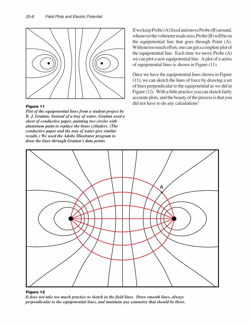
If we keep Probe (A) fixed and move Probe (B) around,whenever the voltmeter reads zero, Probe (B) will be onthe equipotential line that goes through Point (A).Without too much effort, one can get a complete plot ofthe equipotential line. Each time we move Probe (A)we can plot a new equipotential line. A plot of a seriesof equipotential lines is shown in Figure (11).

Once we have the equipotential lines shown in Figure(11), we can sketch the lines of force by drawing a setof lines perpendicular to the equipotential as we did inFigure (12). With a little practice you can sketch fairlyaccurate plots, and the beauty of the process is that youdid not have to do any calculations!

Figure 12It does not take too much practice to sketch in the field lines. Draw smooth lines, alwaysperpendicular to the equipotential lines, and maintain any symmetry that should be there.

Figure 11Plot of the equipotential lines from a student project byB. J. Grattan. Instead of a tray of water, Grattan used asheet of conductive paper, painting two circles withaluminum paint to replace the brass cylinders. (Theconductive paper and the tray of water give similarresults.) We used the Adobe Illustrator program todraw the lines through Grattan's data points.

A

25-9

Exercise 2The equipotential plot of Figure (11) and the field linesof Figure (12) were taken from a student project. Thefield lines look like the field of two point charges +Q and-Q separated by a distance r. But who knows what ishappening in the shallow tank of water (or a sheet ofconducting paper)? Perhaps the field lines more nearlyrepresent the field of two line charges +λ and -λseparated by a distance r.

The field of a point charge drops off as 1/r2 while the fieldof a line charge drops off as 1/r. The point of the exerciseis to decide whether the field lines in Figure (12) (or yourown field plot if you have constructed one in the lab)more closely represent the field of a point or a linecharge.

Hint—Look at the electric field at Point A in Figure (12),enlarged in Figure (13). We know that the field E at PointA is made up of two components, E1 directed away fromthe left hand cylinder, and E2 directed toward the righthand cylinder, and the net field E is the vector sum of thetwo components. If the field is the field of point chargesthen E1 drops off as 1/r12 and E2 as 1/r22 . But if the fieldis that of line charges, E1 drops off as 1/r1 and E2 as

1/r2 . We have chosen Point (A) so that r1, the distancefrom (A) to the left cylinder is quite a bit longer than thedistance r2 to the right cylinder. As a result, the ratio of

E1 to E2 and thus the direction of E, will be quitedifferent for 1 r1 r and 1 r21 r2 forces. This difference is greatenough that you can decide, even from student labresults, whether you are looking at the field of point orline charges. Try it yourself and see which way it comesout.

Figure 13Knowing the direction of the electric field at Point (A)allows us to determine the relative magnitude of thefields E1 and E2 produced by charges 1 and 2 alone.At Point (A), construct a vector E of convenient lengthparallel to the field line through (A). Then decomposeE into component vectors E1 and E2 , where E1 liesalong the line from charge 1 to Point (A), and E2along the line toward charge 2. Then adjust thelengths of E1 and E2 so that their vector sum is E .

E2

2

E1

1E = E + E

A

toward charge 1

toward

charge2

(repulsive)

25-10 Field Plots and Electric Potential

A Field Plot ModelThe analogy between a field plot and a map maker’scontour plot can be made even more obvious byconstructing a plywood model like that shown inFigure (14).

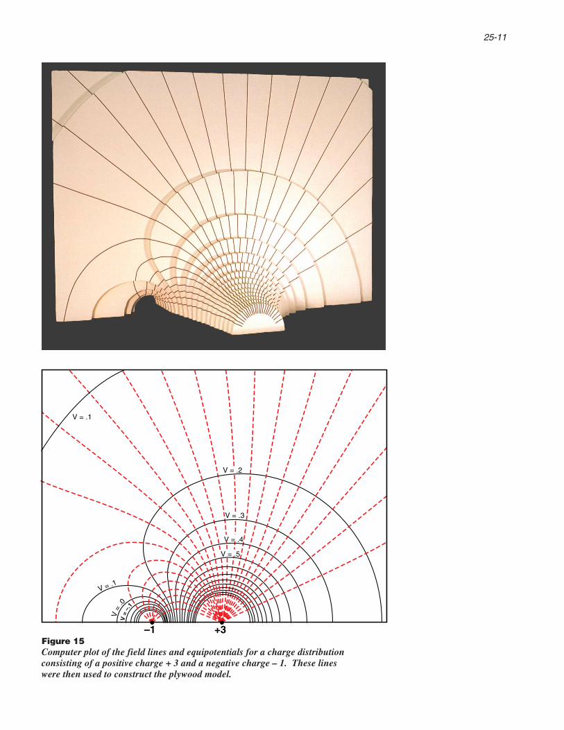
To construct the model, we made a computer plot of theelectric field of charge distribution consisting of acharge +3 and –1 seen in Figure (15). We enlarged thecomputer plot and then cut out pieces of plywood thathad the shapes of the contour lines. The pieces ofplywood were stacked on top of each other and gluedtogether to produce the three dimensional view of thefield structure.

In this model, each additional thickness of plywoodrepresents one more equal step in the electric potentialor voltage. The voltage of the positive charge Q = +3is represented by the fat positive spike that goes uptoward + ∞ and the negative charge q = –1 is repre-sented by the smaller hole that heads down to

– ∞ .

These spikes can be seen in the back view in Figure(14), and the potential plot in Figure (16).

In addition to seeing the contour lines in the slabs ofplywood, we have also marked the lines of steepestdescent with narrow strips of black tape. These lines ofsteepest descent are always perpendicular to the con-tour lines, and are in fact, the electric field lines, whenviewed from the top as in the photograph of Figure (15).

Figure (17) is a plywood model of the electric potentialfor two positive charges, Q = +5, Q = +2. Here we gettwo hills.

Figure 14Model of the electric field in the region of two pointcharges Q+ = + 3, Q– = – 1. Using the analogy to atopographical map, we cut out plywood slabs in theshape of the equipotentials from the computer plot ofFigure 15, and stacked the slabs to form a threedimensional surface. The field lines, which aremarked with narrow black tape on the model, alwayslead in the direction of steepest descent on the surface.

Figure 17Model of the electric potential in the regionof two point charges Q = +5 and Q = +2.

Figure 16Potential plot along theline of the two charges+3, –1. The positivecharge creates an upwardspike, while the negativecharge makes a hole.

–1

+3–.1V

–.2V

–.3V

–.4V

.1V

.2V

.3V

.4V

.5V

.6V

.7V

.8V

.9V

.1.0V

.1.1V

.1. 2V

25-11

V = .1

V = .2

V = .3

V = .4

V = .5

V = .1

V=

–.

1

V=

.0

–1 +3 Figure 15Computer plot of the field lines and equipotentials for a charge distributionconsisting of a positive charge + 3 and a negative charge – 1. These lineswere then used to construct the plywood model.

25-12 Field Plots and Electric Potential

Computer PlotsThere are now many excellent programs that havepersonal computers draw out field plots for variouscharge distributions. In most of these programs youenter an array of charges and the computer draws thefield and equipotential lines. You should practice withone of these programs in order to develop an intuitionfor the field structures various charge distributionsproduce. In particular, try the charge distributionshown in Figure (18) and (19). In Figure (18), we wishto see the field of oppositely charged plates (a positiveplate on the left and a negative one on the right). Thischarge distribution will appear in the next chapter inour discussion of the parallel plate capacitor.

In Figure (19) we are modeling the field of a circle orin 3-dimensions a hollow sphere of charge. Somethingrather remarkable happens to the electric field lines inthis case. Try it and see what happens!

Exercise 3

If you have a computer plotting program available, plotthe field lines for the charge distributions shown inFigures (18,19), and explain what the significant fea-tures of the plot are.

+ –+ –+ –+ –+ –

++

+

++ + +

+

++

Figure 19We have placed + charges around a circle tosimulate a cylinder or sphere of charge. Youget interesting results when you plot the fieldlines for this distribution of charge.

Figure 18The idea is to use the computer to develop an intuitionfor the shape of the electric field produced by variousdistributions of electric charge. Here the parallel linesof charge simulates two plates with opposite charge.

Exercise 4

Figures (20a) and (20b) are computer plots of theelectric field of opposite charges. One of the plotsrepresents the 1/r2 field of 3 dimensional point charges.The other is the end view of the 1/r field of line charges.You are to decide which is which, explaining how youcan tell.

a)

b)

Figure 20Computer plots of 1/r and 1 / r 2 (two dimensionaland three dimensional) fields of equal and oppositecharges. You are to figure out which is which.

25-13

IndexSymbols2D or 3D? equipotential plotting experiment 25-8

CComputer

Plot of electric fieldsField plot model 25-12

Conservative force 25-5Contour map 25-1

EElectric field

Computer plotting programs 25-12Contour map 25-1Equipotential lines 25-3

Electric potentialContour map 25-1Field plots 25-1Of a point charge 25-5Plotting experiment 25-7

Electric voltage. See also VoltageIntroduction to 25-6

EnergyElectric potential energy

Contour map of 25-1Negative and positive 25-4Of a point charge 25-5Plotting 25-7. See also Experiments II: - 1-Potential plotting

Negative and positive potential energy 25-4Voltage as energy per unit charge 25-6

Equipotential lines 25-3Model 25-10Plotting experiment, 2D or 3D? 25-8

Experiments II- 1- Potential plotting 25-7

FField

Plotting experiment 25-7Field lines

Computer plots, programs for 25-12Three dimensional model 25-10

Field plots and electric potential, chapter on 25-1Force

Conservative forces 25-5

LLines, equipotential 25-3

MMap, contour 25-1Model showing equipotential and field lines 25-10

PPlotting

Experiment, electric potential 25-7Potentials and fields. See Experiments II: - 1- Poten-

tial plottingPotential, electric

Contour map 25-1Of a point charge 25-5

Potential energyConservative forces 25-5Electric potential energy

Contour map of 25-1Negative and positive 25-4Of a point charge 25-5Potential plotting 25-7

Negative and positive 25-4Potential plotting. See Experiments II: - 1- Potential

plotting

VVoltage

Electric 25-6

XX-Ch25

Exercise 1 25-5Exercise 2 25-9Exercise 3 25-12Exercise 4 25-12

25-14 Field Plots and Electric Potential

Contents

CHAPTER 25 FIELD PLOTS ANDELECTRIC POTENTIAL

The Contour Map

Equipotential LinesNegative and PositivePotential Energy

Electric Potentialof a Point Charge

Conservative Forces

Electric VoltageA Field Plot ModelComputer Plots

Index