322 รวมบทความวิชาการ 22 drc018.pdf · 322...

DRC018

322 รวมบทความวชิาการ เล่มท่ี 1 การประชุมวชิาการเครือข่ายวศิวกรรมเคร่ืองกลแห่งประเทศไทยครังท่ี 22

The 22nd Conference of Mechanical Engineering Network of Thailand 15-17 October 2008, Thammasat University, Rangsit Campus, Pathum Thani, Thailand

Analytical Kinematics and Dynamics for 5 axis H-4 parallel Manipulator

Kummun Chooprasird and Viboon Sangveraphunsiri* Robotics and Manufacturing Lab.

Department of Mechanical Engineering,Faculty of Engineering, Chulalongkorn University Bangkok 10330, Thailand.

*E-mail: [email protected] Abstract This work presents analysis and design of an unique hybrid 5 degree-of-freedom robotic manipulator based on a H-4 Family of Parallel Mechanisms with three degree-of-freedom in translational movements and one degree-of-freedom in rotational movement (orientation angle) at the tool tip of the arm together with another degree-of-freedom coming from a single axis rotating table. This manipulator can be used in a rapid prototype application for cutting soft materials. Forward or direct kinematics, inverse kinematics and Jacobian of the purposed configuration are derived in detail as well as equations of motion of the manipulator arm. The equations of motion or the dynamic model are derived from Lagrangian formulation and are shown to be suitable in real-time feedback controls. The accuracy of the kinematics, forward and inverse, Jacobian, and the dynamic model derived in this work are assured by comparing the results obtained from using MATLAB developed in this work with the result from the ADAMS solver with the manipulator arm 3D solid model data. The comparisons between the two numerical results are very promising. Keywords: H-4 Parallel Robot, Resolve acceleration, Lagrangian formulation 1. Introduction Many advantages of the parallel mechanism robots over serial mechanism, such as structural stiffness, load capacity, accurate precision, speed and acceleration performance, induce the parallel manipulator to the topics of research activities in the academic community for several years since the 6-DOF parallel mechanism for flight simulator proposed by Gough and Stewart. Although the disabilities due to the parallel configurations are the small working volume and small movement for orientation to reach a workpiece, the benefits of these mechanisms have still been taking in development continuously in fields of robotic. Recently, many applications utilize the parallel mechanisms in industries such as high-speed laser machine using three RUU parallel chains (RUU: Revolute-Universal-Universal) by Delta Group, 3-DOF (RUU chains) the FlexPicker IRB 340 for high-speed picking and packing

applications by ABB, 6-DOF “Hexapod” as consisted of 6 UPS parallel chains (UPS: Universal-Prismatic-Spherical). As known before, the minimum requirement to give maximum flexibility in between tool and workpiece orientation is five degrees of freedom. It means that the tool can be oriented in any angle relative to workpiece. In the case where a part with complex surfaces, 3-DOF manipulator cannot perform good enough surface cutting. Or event worst, 3-DOF manipulator can not fulfill all the surfaces of the part. This is not the case for 5-DOF manipulator. In present time, the manufacturing industries are widely known the 5-DOF in parallel structure than before. Besides the advantages mentioned above, the motion characteristics are also preferable such as the errors in the arms are averaged instead of build up as in series structure, the load is distributed to all arms, low inertia due to actuators are mount on a fixed base. The purposed configuration is good for a rapid prototype application in the form of a master-slave application with force control algorithms. Due to multiple close-chain links make the dynamic analysis of parallel manipulators more complicated than serial manipulators. And dynamic analysis of various types of parallel mechanisms has been studied by many researchers. Do and Yang, 1988; Guglielmetti and Longchamp, 1994; Tsai and Kohli, 1990 formulated dynamic models from Newton-Euler method. While Lebret 1993; Miller and Clavel, 1992; Miller and Clavel, 1992; Pang and Shahingpoor, 1994, used Lagrange Equations method. And virtual work method is studied by Codourey and Burdet, 1997; Miller, 1995; Tsai,1998; Wang and Gosselin, 1997; Zhang and Song, 1993. To obtain the dynamic model by using Newton-Euler formulation, the equations of motion of each body need to be written which leads to a large number of equations and consumes large computation time when used in a real-time control system. Unnecessary computation of reaction forces as done in the Newton-Euler formulation are eliminated in the Lagrangian formulation. Additional coordinates along with a set of Lagrangian and some model simplification make the Lagrange formulation more efficient than Newton-Euler formulation. In this paper we derive the dynamic model of the H-4 parallel

รวมบทความวชิาการ เล่มท่ี 1 การประชุมวชิาการเครือข่ายวศิวกรรมเคร่ืองกลแห่งประเทศไทยครังท่ี 22 323

robot by using the Lagrangian. Sangveraphunsiri has been working on the kinematics analysis for sometimes as shown in [6], [8] and [9], some of the works here are based on those works. The intention of this paper is to design and evaluate the kinematics of a 5-DOF manipulator based on the H-4 family parallel structure together with one rotational table as shown in Figure 1. Lagrange formulation has been introduced to analyze dynamics of H-4 manipulator. The computer simulation using the commercial software (ADAMS solver), with the solid model data of the system, is carried out to compare the results from the dynamic model derived. From the simulation results, it is shown that the complexity and the performance of this kind of configuration are suitable for complex surface machining application with or without cutting force control. Tele-operation with force reflecting control can also be implemented with this configuration. 2. Design Consideration

The desired H-4 parallel robot must have at least 4-DOF which will produce 3 translation motions and 1 rotary motion. In order to have large rotational movement in y-axis, the mechanism will consist of two mechanical chains connect to two separated platforms. Each chain has two degrees of freedom moving along the x-axis of the platform as shown in Figure 1 and Figure 2. The work volume is depends on the 4 parameters as the length of limb, the size of platform, 2c, the different between machine frame and platform, (b – a), and the offset between two separated platform, 2d. The 4 variables (l1, l2, l3, and l4) are used for specifying the position in (x, y, z) and rotation in y-axis of the tool tip.

Figure 1. Proposed design

3. Kinematics Modeling In this section, we derive the relationships between the joint variables of the 5-DOF of the mechanism,

and working coordinate system

as shown in Figure 1

and Figure 2, where , ,w wI J and wK are the directional

cosine of the working frame .

Inverse Kinematics Typically, working paths will be defined in Cartesian space or the working coordinate system. Inverse kinematics is used for obtaining the joint commands from the specified working paths.

Figure 2. Robot joint configuration

From Figure 2, vector C1B1 and C1B2 are symmetry

about ZcYc-plane if θ = 0 and vector OcC1 and OcC3 point to opposite direction. So, inverse position relationships can be obtained as follow: 2 2 2

1,2 ( ) ( )a a al x w R y e z ge= + ± - - - - From geometrical restrictions, we can conclude that 2 2 2

1 ( ) ( )a a al x w R y e z ge= + + - - - - (1)

2 2 22 ( ) ( )a a al x w R y e z ge= - - - - - - (2)

The coordinate ( ), ,a a ax y z represents the vector

position of point C1 with respect to origin of the link 1l or

2l . The relationship between tool-tip coordinate frame,

{ }, ,x y z , and center coordinate frame, { }, ,c c cx y z , can be derived as following

( ) sin( )

( 2 ) sin( )c

a L

Lx

x

T c

T c

x

q

q= + + × -

= + + × - (1a)

( )ay y b a= - + + (1b)

( 2 ) cos( )a Lz T cz dq+ + × -= -- (1c) Similarly, the others actuator-end effecter position

relationship become,


2 2 2

3 ( ) ( )b b bl x w R y e z ge= + + - - - - (3)

2 2 24 ( ) ( )b b bl x w R y e z ge= - - - - - - (4)

where ( ), ,b b bx y z is coordinate of the point C3 with

respect to origin of the link 3l or 4l as shown in Figure 2 and it can be shown that

( ) ( )sin sin( )Lc L b Tx x T c xq q= + + - = + × - (2a)

( )c byy by a= = + - (2b) ( )cosb Lz z d T q- = + + - (2c) From equation (3), (4), and (2a)-(2c), , ,b bx y and

bz are always positive while cz and z are always negative. The angle q is negative with respect to the y-direction shown in Figure 2. Figure 3 shows the workpiece coordinate system ( ). ,w w wx y z and the reference coordinate system (XYZ). Using geometric transformation to transform the workpiece coordinate to the reference coordinate as follows:

where T means translation and R means rotation. We will get:

1O

w OwX x x p= + + (3a)

1 2

1( ) cos ( ) sinO Ow Ow w OY y y z za a= + × - + ×

(3b)

1 2

1( ) sin ( ) cosO Ow Ow w OZ y y z z ha a= + × + + × - (3c)

Where 1 1 1

w w w

O O OO O Ox y z are the coordinates with the origin at

wO written in frame 1O , and 21

OOz is the coordinate of the

origin 1O in frame 2O .

Figure 3. The Workpiece Table Reference Position and

Intermediate Reference Systems

During cutting, the end of the tooltip ({P}) has to be located on the surface of the workpiece. So from equations (1), (1a), (1b), (1c) and (3a) - (3b), finally, the solution for 1l can be written as following:

11

2 1 2 21

1 2 21

( ) ( 2 ) sin( )

[ ( ) cos ( ) sin ]

[ ( ) sin ( )cos ( 2 )cos( ) ]

Ow Ow L

O Ow Ow w O

O Ow Ow w O L

l x x p T c w

R y y z z b a e

y y z z h T c d ge

q

a a

a a q

= + + + + + +

- - + + + - + -

- + - + + - + + -

-

Similarly, we can solve 2l , 3l , and 4l as follows:

12

2 1 2 21

1 2 21

( ) ( 2 )sin( )

[ ( )cos ( )sin ]

[ ( )sin ( )cos ( 2 )cos( ) ]

Ow Ow L

O Ow Ow w O

O Ow Ow w O L

l x x p T c w

R y y z z b a e

y y z z h T c d ge

q

a a

a a q

= + + + + - -

- - + + + - + -

- + - + + - + + -

-

13

2 1 2 21

1 2 21

( ) sin( )

[( ) cos ( ) sin ]

[ ( ) sin ( ) cos cos( ) ]

Ow Ow L

O Ow Ow w O

O Ow Ow w O L

l x x p T w

R y y z z b a e

y y z z h T d ge

q

a a

a a q

= + + + + +

- + - + - + -

- + - + + - - -

-

14

2 1 2 21

1 2 21

( ) sin( )

[( )cos ( ) sin ]

[ ( ) sin ( )cos cos( ) ]

Ow Ow L

O Ow Ow w O

O Ow Ow w O L

l x x p T w

R y y z z b a e

y y z z h T d ge

q

a a

a a q

= + + + - -

- + - + - + -

- + - + + - - -

-

For the tooltip orientation, it has to be coincident with

the direction-cosine of cutting position on the workpiece surface.

Figure 4. ToolTip orientation and workpiece direction cosine

The unit vector of the normal plane at cutting location

of a workpiece surface can be written as w w w w w wI i J i K k+ + , where , ,w w wI J K are the direction

cosine. So, the orientation can be obtained as follows:

; 2 wI I=

2 22 ( ) cos( )w wJ J K pa= + +

2 22 ( ) sin( )w wK J K pa= + +

From these equations, the solution of a and q will be:


where 90 90a- £ £o o

where 90 90q- £ £o o

Forward or Direct Kinematics

In the previous section, we derive the robot variables, 1 2 3 4, , ,l l l l and a from a given position and orientation on

a workpiece surface. In this section we will derive the tooltip position and orientation from a given set of robot variables. The robot variables 1 2 3 4, , ,l l l l and a , shown in Figure 3a and 3b, will be used to define new variables depends as,

1 2 3 4

1 2 1 1 2 2 3 4, , ,

2 2

l l l lr r d l l d l l

+ += = = - = -

So, the rotation angle of the platform can readily be determined as

( )222 14

cos2

c r rc

q- -

= (4)

Position relationship can be obtained by manipulating expression (1), (2), (3 ) and (4) which lead to, ( ) ( ) ( )

( )

2 2 22 21 3

22

2 2 2

2( ) 2 cos

a b c

c

l x w l x w R y b a e

z ge c dq

- - + - - = - - - +

- + - × - (4a)

( ) ( ) ( )

( )

2 22 4 4

4( ) cosa b c

c

l x w l x w y b a e

z ge c dq

- - - - - = - - -

- + × -

(4b)

Figure 5. New variables defined

Figure 6. New variables defined

Simplify the expressions above, using the new

variables shown in Figure 5-6, we will have

( ) ( )2

2 2 12 1 4a a

dl x l x- = - =

( ) ( )2

2 2 24 3 4b b

dl x l x- = - =

From equation (1a) and Figure 5-6, the movement in x direction is easily obtain as

(5)

which finally, we will obtain

( )

2 21 2 1 24 ( ) 16( . cos )( )

16c

cd d w d d d c z gey y

a b eq- - - - - += =

- - (6)

We can also obtain cz by substitutes the above

expression in (4b), which leading to 2nd degree polynomial equation as:

(7)

From equation (7), we can solve with simple formula:

2 4

2cB B A Cz

A- ± -= (8)

Due to configuration of robot, the solution in cz is always in negative. Therefore, the coefficient , ,A B C can be found as:


( )

( )( )

2

2

2 21 2 1 2

2

512. .( cos )4.128

32( cos ) 4 ( )128

ge d cB gea b e

d c d d w d da b e

q

q

-= +- -

- - - --

- -

( )

( )( )

( )( )

( )( )

2 2 2

2

2 21 2 1 2

2

22 21 2 1 2 2 2 2

1 22

2 21 2 22 2

16 ( cos ) .128

32. .( cos ) 4 ( )128

4 ( )2 ( ) 2. 2

128

2 2 4 ( ) 2( . cos )4

d c geCa b e

ge d c d d w d da b e

d d w d dw w d d ge e

a b e

d dR b a e a b c d

q

q

q

-=- -

- - - --

- -

- - -+ + - + + +

- -

++ - + - - - + -

Knowing cz from equation (8), z can be found as

( ) cosc Lz z c T q= - + Using geometric transformation to transform the

reference coordinate to the workpiece coordinate as follows:

So, tool-tip contact point on the workpiece surface can be obtained by equations as follow:

1

Oww Ox x p x= + +

1cos( ) ( ) sin( ) Oww Oy y z h ya a= × + + × +

12( ) cos( ) sin( ) O

w Oz z h y za a= + × - × + Finally, we can find direction cosine of the workpiece cutting location, or tool-tip contact point, from angle θ and α as:

2

111

tan

wI

q

= ±+

where ( ) ( )wsign I sign q=

( ) ( )2 2

11 tan 1 tan (90 )

wJq a

= ±+ × + -

where ( ) ( )wsign J sign a=

( ) ( )2 2

tan(90 )1 tan 1 tan (90 )

wK aq a

-=+ × + -

where ( )wsign K = + In order to obtain the velocity relationship between

the joint variable and the working coordinate, we apply the differential position relationship instead. Or knowing the velocity vector on the platform relative to the rotating table directly, we can obtain the relationship of the velocity of the tool attached relative to the moving table which represents by

and the

actuator input denoted by q as following: Moving platform velocity,

Then, the velocity at point B related to that of point

A, · = ·i i Ai i i BiA B V A B V

According to [5], the Jacobian matrix of the machine can be written in the form as

where 1-=J A B So,

(9)

To derive the singularity, we consider only H-4 parallel manipulator which matrix A and B reduce to 4x4 matrix as follows[9]:

At this point one can derive the singularity of the

manipulator, according to [5] and [1], by finding the determinant of matrix A and B. In this case we interests in singularity of type 2 [5] which occurs within workspace. From the set of equations (9), substitute all parameters into the matrix yield,

(10)


where,

The analytical form of the determinant of matrix B is

found to be,

(11) From observation of equation (11), the singularity occurs at following cases,

1) 1 2l l- or 3 4l l- is zero. This indicate that lines

1 1A B and 2 2A B or 3 3A B and 4 4A B are coincide.

2) cos 0q = or 90q = ± o . This means that the moving platform is parallel to x-axis.

3) ( ) ( )cos 0y d z b aq- - - = Þ ( )( )

cosy dzb a

q-=-

,

which shows that the planes formed by lines 1 1A B and 2 2A B and by 3 3A B and 4 4A B are in

parallel.

(1), (2)

(3)

Figure 7. Singularity Configurations

From equation , we can find Jacobian matrix (J) by differentiate inverse kinematics equation as follow:

, where

and

Where 2 2 2R B CA --=

Where 1 1 12 2 2R B CA --=

11 2

1( ) cos ( ) sinO Ow wO w Oy y z z b a eB a a+ - + - + -=

11 2

1( ) sin ( ) coscos( )

O Ow wO w O

L

y y z zh T d ge

C a aq

+ + +- + + +

=

4. Analytical Dynamics Model In this section, the conservative Lagrange’s equation is used to obtain the dynamic model of the closed-chain H-4 type from the forward kinematics derived earlier. For conservative system, the well-known generalized Lagrange’s equation of coordinates qi, with generalized force Qi , can be written as:


The robot manipulator consists of 5 components as shown in Figure 8 which can be detailed as following,

-Milling Head or Platform 1 part. -Connecting Head 2 parts. -Arm or link 8 parts. -Linear joint 4 parts. -Universal cross (U-joint) 16 parts.

We can write the Lagrange’s equation of each component above. Considering the platform component, the Lagrange’s equation based on the coordinate of the linear joint li of 4-DOF can be derived as following:

For the two connecting heads, the Lagrange’s equation will be:

For the eight robot arms, the Lagrange’s equation will be: (14)

where

For the four linear joints, the Lagrange’s equation will be:

For all universal crosses, the Lagrange’s equation will be:

By Summing equations (12)-(16), we will get equation of motion of the system as: (16)

According to the Figure 8, the parameters on connected head (CH) is found as: ge = 104mm , e = 23.75mm, w = 35mm


Figure 8. Robot Components

The parameters in equation (12a)-(12c) can be found as follows:

Due to the coefficient , ,A B C in equation (8), we can rearrange in terms of joint parameter l1 l2 l3 l4 together with substitute the value of parameters ge = 104 , e= 23.75, w = 35 and we can obtain

The time derivative of A,B,C can be found as


And the second time derivative of A,B,C can be found as


For the platform component as shown in equations (12) and (12a)-(12c), we need to obtain the derivative with respect to li of the first and second time derivative obtained above by applying chain rule. Then, rearranging the expressions, we will get translational force on each joint due to mass and inertia of milling head. We continue to do the same procedure on the remaining components as shown in the equations (13), (14), (15) and (16). Finally, total force (Fi) can be obtained by summing all forces which are generated from masses and moments of inertia of other components. 5. Simulation Results The dynamic model obtained from previous section is implemented in MATLAB in order to compare the numerical solutions with the commercial dynamics software such as the ADAMS solver. The model parameters used in the simulation are Tl= 163 mm, c= 37.5 mm, R=587mm, b=57.25mm, a= 215mm, h= 1024.5mm, p=720 mm, d=37.5mm, Ec= 22.93 mm. We use materials as mild steel for all components. So, mass properties and moments of inertia can be found as follows:

2

2,

2,

2

14.0881

9.36853

2.7194

4.65962

0.28739

94625.076

105660

105415

60.3645

MH

CH

Am

LJ

UC

MHy

XX Am

Y Y Am

UCy

m kg

m kg

m kg

m kg

m kg

I kgmm

I kgmm

I kgmm

I kgmm

=

=

=

=

=

=

=

=

=

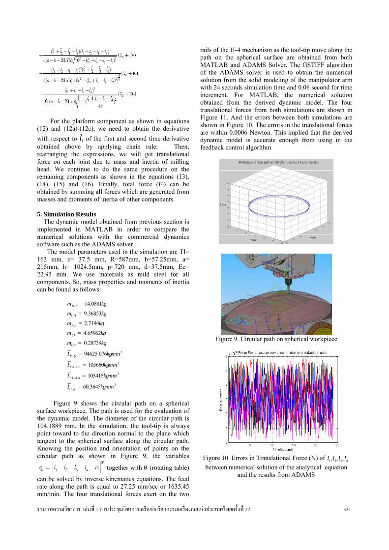
Figure 9 shows the circular path on a spherical surface workpiece. The path is used for the evaluation of the dynamic model. The diameter of the circular path is 104.1889 mm. In the simulation, the tool-tip is always point toward to the direction normal to the plane which tangent to the spherical surface along the circular path. Knowing the position and orientation of points on the circular path as shown in Figure 9, the variables

together with θ (rotating table)

can be solved by inverse kinematics equations. The feed rate along the path is equal to 27.25 mm/sec or 1635.45 mm/min. The four translational forces exert on the two

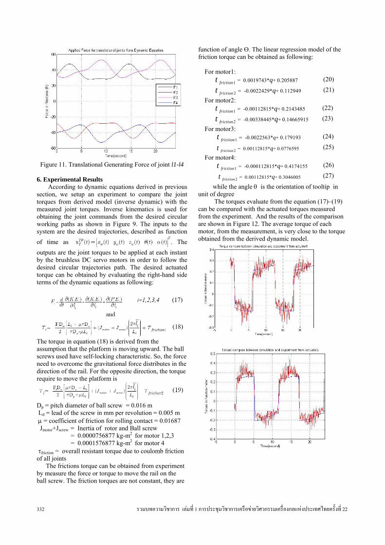
rails of the H-4 mechanism as the tool-tip move along the path on the spherical surface are obtained from both MATLAB and ADAMS Solver. The GSTIFF algorithm of the ADAMS solver is used to obtain the numerical solution from the solid modeling of the manipulator arm with 24 seconds simulation time and 0.06 second for time increment. For MATLAB, the numerical solution obtained from the derived dynamic model. The four translational forces from both simulations are shown in Figure 11. And the errors between both simulations are shown in Figure 10. The errors in the translational forces are within 0.0006 Newton. This implied that the derived dynamic model is accurate enough from using in the feedback control algorithm

Figure 9. Circular path on spherical workpiece

Figure 10. Errors in Translational Force (N) of 1 2 3 4, , ,l l l l between numerical solution of the analytical equation

and the results from ADAMS


Figure 11. Translational Generating Force of joint l1-l4

6. Experimental Results According to dynamic equations derived in previous section, we setup an experiment to compare the joint torques from derived model (inverse dynamic) with the measured joint torques. Inverse kinematics is used for obtaining the joint commands from the desired circular working paths as shown in Figure 9. The inputs to the system are the desired trajectories, described as function of time as . The outputs are the joint torques to be applied at each instant by the brushless DC servo motors in order to follow the desired circular trajectories path. The desired actuated torque can be obtained by evaluating the right-hand side terms of the dynamic equations as following:

The torque in equation (18) is derived from the assumption that the platform is moving upward. The ball screws used have self-locking characteristic. So, the force need to overcome the gravitational force distributes in the direction of the rail. For the opposite direction, the torque require to move the platform is

Dp = pitch diameter of ball screw = 0.016 m Ld = lead of the screw in mm per revolution = 0.005 m μ = coefficient of friction for rolling contact = 0.01687 Jmotor+Jscrew = Inertia of rotor and Ball screw = 0.0000756877 kg-m2 for motor 1,2,3 = 0.0001576877 kg-m2 for motor 4 τfriction = overall resistant torque due to coulomb friction of all joints

The frictions torque can be obtained from experiment by measure the force or torque to move the rail on the ball screw. The friction torques are not constant, they are

function of angle Ө. The linear regression model of the friction torque can be obtained as following: For motor1: 1 0.0019743* + 0.205887friction qt = (20) 2 -0.0022429* + 0.112949friction qt = (21) For motor2: 1 -0.00112815* + 0.2143485friction qt = (22) 2 -0.00338445* + 0.14665915friction qt = (23) For motor3: 1 -0.0022563* + 0.179193friction qt = (24)

2 0.00112815* + 0.0776595friction qt = (25) For motor4:

1 -0.000112815* + 0.4174155friction qt = (26)

2 0.00112815* + 0.3046005friction qt = (27)

while the angle θ is the orientation of tooltip in unit of degree The torques evaluate from the equation (17)–(19) can be compared with the actuated torques measured from the experiment. And the results of the comparison are shown in Figure 12. The average torque of each motor, from the measurement, is very close to the torque obtained from the derived dynamic model.


Figure 12. Compare torques between simulation model

by derived equation and experiment.

7. Conclusion In this paper, we presented the kinematics analysis,

Jacobian and the Dynamic Model of the 5-DOF parallel mechanism design base on H-4 family. The forward and inverse kinematics analysis are presented. Singularities analysis is shown only for the H-4 type. The dynamic equations are derived from the Lagrangian formulation. The numerical results of the analysis of kinematics, Jacobian and the dynamic model are compared with numerical results from a popular commercial software, the ADAMS solver, using the solid model data. This is to assure the accuracy the derived model and possibility of using it in the feedback system. Friction models obtained from the experiment are used to compensate the actual friction of the system in the resolve acceleration control strategy.

References [1]. Monsarrat, B., Gosselin, C. M. Singularity Analysis

of a Three-Leg 6Dof parallel Grassmann Line Geometry. International Journal of Robotics Research vol.20 no.4, April 2001, pp. 312-326.

[2]. Tsai, L. W. Robot Analysis-The Mechanics of Serial and Parallel Manipulators. John Wiley & Sons, 1999.

[3]. Clavel, R., "Conception d'un robot parallèle rapide à 4 degrés de liberté," Ph.D. Thesis, EPFL, Lausanne, Switzerland, 1991.

[4]. Pierrot, F. H4_a new family of 4-DOF parallel robots. IEEE/ASME Advanced Intelligent

Mechatronics Conf. Proc. Atlanta USA, September 1999, pp. 508-513.

[5]. Gosselin, C. M., Angeles, J. Singularity analysis of closed-loop kinematics chains. IEEE Transactions on Robotics and Automation vol. 6 no. 3, June, 1990. pp. 281-290.

[6]. Sangveraphunsiri,V. and Tantawiroon N., Novel Design of a 4 DOF parallel Robot., 2003 JSAE Annual Congress, Yokohama, Japan, May21-23, 2003.

[7]. Dumitru Olaru, George C. Puiu, Liviu C. Balan, Vasile Puiu, A New Model to Estimate Friction Torque in a Ball Screw System. Product Engineering Springer Netherlands, page333-346,2005

[8]. Viboon Sangveraphunsiri and Prasartporn Wongkumchang, Design and Control of a Stewart Platform, the 15th National Conference of Mechanical Engineering,2001, (in Thai).

[9]. Viboon Sangveraphunsiri and Tawee Ngamvilaikorn, Design and Analysis of 6 DOF Haptic Device for Teleoperation Using a Singularity-Free Parellel Mechanism, Thammasat International Journal of Science and Technology vol.10 No.4 October-December 2005,pp. 60-69.

322 รวมบทความวิชาการ 22 drc018.pdf · 322...

Documents