37470595 water jet propulsion
TRANSCRIPT

Numerical Analysis of a
Waterjet Propulsion System
Norbert Willem Herman Bulten

Acknowledgement: The research described in this thesis was supported by
Wärtsilä Propulsion Netherlands B.V.
Cover: Michelle TjelpaPhoto: Bram KruytPrinting: Printservice Technische Universiteit Eindhoven
Copyright © 2006 by N.W.H. Bulten, The NetherlandsAll rights reserved. No part of this publication may be reproduced, stored in a retrieval system or transmitted in any form or by any means, electronically, meachanically, by pho-tocopying, recording, or otherwise, without the written permission of the author.
A catalogue record is available from the Library Eindhoven University of TechnologyISBN-10: 90-386-2988-5ISBN-13: 978-90-386-2988-9

Numerical Analysis of a
Waterjet Propulsion System
PROEFSCHRIFT
ter verkrijging van de graad van doctor aan deTechnische Universiteit Eindhoven, op gezag van de Rector Magnificus, prof.dr.ir. C.J. van Duijn, voor een
commissie aangewezen door het College voor Promoties in het openbaar te verdedigen
op woendag 15 november 2006 om 16.00 uur
door
Norbert Willem Herman Bulten
geboren te Winterswijk

Dit proefschrift is goedgekeurd door de promotoren:
prof.dr.ir. J.J.H. Brouwersenprof.dr.ir. H.W.M. Hoeijmakers
Copromotor:dr. B.P.M. van Esch

Numerical analysis of a waterjet propulsion system 1
Table of contents
Chapter 1 Introduction ................................................................ 51.1 Waterjet layout................................................................................ 61.2 Relation of waterjet propulsion system to other turbo machinery ... 71.3 Aim of the analysis........................................................................ 101.4 Outline of this thesis ..................................................................... 111.5 Nomenclature ............................................................................... 121.6 References ................................................................................... 12
Chapter 2 Waterjet propulsion theory ..................................... 152.1 Characteristic velocities in a waterjet system ............................... 16
2.1.1 Wake fraction .................................................................... 172.1.2 Inlet velocity ratio ............................................................... 202.1.3 Jet velocity ratio ................................................................. 212.1.4 Summary ........................................................................... 22
2.2 General pump theory .................................................................... 222.2.1 Dimensionless performance parameters ........................... 222.2.2 Pump geometry parameters .............................................. 242.2.3 Cavitation parameters ....................................................... 252.2.4 Correlation with propeller performance parameters .......... 26
2.3 Thrust ........................................................................................... 272.3.1 General thrust equation ..................................................... 272.3.2 Open propeller thrust ......................................................... 282.3.3 Waterjet thrust ................................................................... 302.3.4 Concluding remarks ........................................................... 34
2.4 Pump head ................................................................................... 342.5 Overall propulsive efficiency......................................................... 37
2.5.1 Cavitation margins ............................................................. 392.5.2 Limitations in specific speed .............................................. 402.5.3 Limitations in jet velocity ratio ............................................ 412.5.4 Limitation of power density ................................................ 42
2.6 Waterjet selection ......................................................................... 432.7 Closing remark.............................................................................. 442.8 Nomenclature ............................................................................... 442.9 References ................................................................................... 46
Chapter 3 Non-uniform distribution of pump entrance velocityfield .......................................................................... 49
3.1 Representation of non-uniform velocity distribution...................... 49

2
.
3.1.1 Experimental set-up ........................................................... 503.1.2 Non-dimensional representation ........................................ 523.1.3 Two-dimensional representation ........................................ 52
3.2 Local flow rate fluctuations............................................................ 533.3 Impeller velocity triangles.............................................................. 553.4 Origin of the non-uniform velocity distribution............................... 57
3.4.1 Boundary layer ingestion ................................................... 573.4.2 Deceleration of the flow ..................................................... 583.4.3 Obstruction of the flow due to the shaft ............................. 593.4.4 Bend in the inlet duct ......................................................... 603.4.5 Closing remark ................................................................... 60
3.5 Non-uniform inflow velocity distributions in other turbo machinery603.6 Nomenclature................................................................................ 613.7 References.................................................................................... 62
Chapter 4 Mathematical treatment ...........................................634.1 Requirements of mathematical method ........................................ 63
4.1.1 Incompressibility ................................................................ 644.1.2 High Reynolds number ...................................................... 644.1.3 Time dependency .............................................................. 654.1.4 Non-uniformity of impeller inflow ........................................ 654.1.5 Tip clearance flow .............................................................. 664.1.6 Final remarks ..................................................................... 67
4.2 Conservation laws......................................................................... 674.3 Reynolds Averaged Navier-Stokes (RANS) flow .......................... 68
4.3.1 Reynolds averaging ........................................................... 684.3.2 Eddy viscosity turbulence models ...................................... 70
4.4 Two-dimensional test cases.......................................................... 754.4.1 Isolated NACA 0012 profile ............................................... 754.4.2 Cascades with NACA 65-410 profiles ................................ 804.4.3 Sensitivity of errors in drag on thrust and torque ............... 82
4.5 Nomenclature................................................................................ 854.6 References.................................................................................... 86
Chapter 5 Numerical analysis of waterjet inlet flow ...............895.1 Review of CFD analyses on waterjet inlets................................... 895.2 Geometry and mesh generation ................................................... 915.3 Numerical approach...................................................................... 94
5.3.1 Boundary conditions .......................................................... 945.3.2 Fluid properties .................................................................. 955.3.3 Discretisation and solution algorithm ................................. 95
5.4 Validation with experimental data ................................................. 96

Numerical analysis of a waterjet propulsion system 3
5.4.1 Comparison of static pressure along the ramp centre line 975.4.2 Comparison of cavitation inception pressure at cutwater 1015.4.3 Comparison of total pressure at impeller plane ............... 1055.4.4 Comparison of velocity field at impeller plane ................. 1085.4.5 Results obtained with k-ω turbulence model ................... 1135.4.6 Mesh convergence study ................................................. 1155.4.7 Closing remarks ............................................................... 117
5.5 Analysis of the suction streamtube............................................. 1175.5.1 Visualisation of suction streamtube ................................. 1185.5.2 Determination of suction streamtube shape .................... 118
5.6 Evaluation of wall shear stress ................................................... 1235.7 Nomenclature ............................................................................. 1255.8 References ................................................................................. 125
Chapter 6 Numerical analysis of waterjet pump flow ........... 1276.1 Geometry and mesh generation ................................................. 1276.2 Numerical approach.................................................................... 131
6.2.1 Boundary conditions ........................................................ 1316.2.2 Fluid properties ................................................................ 1326.2.3 Impeller rotation ............................................................... 1326.2.4 Calculation of global pump performance ......................... 132
6.3 Validation with experimental data ............................................... 1346.3.1 Quasi-steady flow calculations with the MFR method ..... 1356.3.2 Transient flow calculations with moving mesh ................. 1386.3.3 Rotor-stator interaction forces ......................................... 144
6.4 Influence of non-uniform axial inflow .......................................... 1476.4.1 Pump performance for non-uniform inflow ...................... 1476.4.2 Background of radial forces acting on the impeller .......... 1486.4.3 Flow rate fluctuations in the impeller channel .................. 1496.4.4 Radial forces for non-uniform inflow ................................ 1506.4.5 Concluding remark .......................................................... 155
6.5 Nomenclature ............................................................................. 1556.6 References ................................................................................. 156
Chapter 7 Analysis of a complete waterjet installation ........ 1597.1 Generation of the numerical model............................................. 1597.2 Evaluation of volume flow rate.................................................... 1607.3 Evaluation of waterjet thrust ....................................................... 161
7.3.1 Integration of solid wall forces ......................................... 1617.3.2 Momentum balance ......................................................... 1637.3.3 Results ............................................................................ 163
7.4 Evaluation of required power ...................................................... 164

4
.
7.5 Analysis of vertical force on waterjet structure............................ 1657.6 Pressure distribution on streamtube surface .............................. 168
7.6.1 Evaluation of momentum balance in vertical direction ..... 1687.6.2 Calculation of vertical force on streamtube ...................... 1697.6.3 Concluding remark ........................................................... 171
7.7 Nomenclature.............................................................................. 1717.8 References.................................................................................. 172
Chapter 8 Concluding remarks ...............................................1738.1 Conclusions ................................................................................ 173
8.1.1 Theory of thrust prediction for waterjet systems .............. 1738.1.2 Numerical aspects ........................................................... 1748.1.3 Waterjet inlet flow characteristics .................................... 1748.1.4 Waterjet mixed-flow pump analyses ................................ 175
8.2 Recommendations...................................................................... 1758.2.1 Research topics for marine propulsion systems .............. 1758.2.2 Application of RANS methods ......................................... 176
Appendix A Stability of non-uniform ..velocity distribution 177A.1 Test case with non-uniform pipe flow.......................................... 178A.2 References.................................................................................. 180
Appendix B Fourier analyses of transient flow calculations 181
Summary ...................................................................................189
Samenvatting ...........................................................................193
Dankwoord ...............................................................................197
Curriculum Vitae ......................................................................199

Numerical analysis of a waterjet propulsion system 5
Chapter 1 Introduction
The desire to travel faster and further is probably as old as mankind itself.There has been an enormous development in the way people use to travelfrom one place to another. At first it was only over land, and later also oversea. And since about a century is it possible to travel through air as well.
Achievements in automotive and aerospace technology are widelyrecognized. But probably, most readers do not realize the substantialdevelopment in high speed ship transportation. At the end of the 20th century,fast ferry catamarans sailing at 50 knots (equivalent to about 90 km/h) were incommercial service all over the world. However, this type of vessel hadentered the market less than two decades before.
The considerable development in the high speed craft can be partlycontributed to the application of waterjet propulsion systems. Currently usedstern mounted waterjets are based on principles as applied by Riva Calzoniin 1932 [1]. However, the first type of waterjet propulsion was inventedalready 300 years earlier, by David Ramseye [2]. He stated in 1630 in EnglishPatent No. 50 that he was able ‘to make Boates, Shippes and Barges to goeagainst Stronge Winde and Tyde’. It is supposed that he had a waterjet inmind for the propulsion, since at that time there was a great interest in usingsteam to raise water and to operate fountains. In 1661, English patent no.132 was granted to Thomas Toogood and James Hayes for their invention of’Forceing Water by Bellowes [...] together with a particular way of Forceingwater through the Bottome or Sides of Shipps belowe the Surface or Toppe ofthe Water, which may be of siguler Use and Ease in Navagacon’. Thisconcept was based on a waterjet without a doubt. However, they did not
6
Chapter 1. Introduction
manage to develop a working prototype. This invention and the subsequentdevelopment of the waterjet until 1980 is described in much more detail byRoy [3]. From 1980 onwards the use of waterjets in commercial applicationsreally started to grow [4].
At the start of the 21th century the sizes of installed waterjets have increasedto diameters of about 3 meter. This has led to installed powers of 25 MW perinstallation. Luxury high speed motor yachts have achieved ship speeds wellabove 65 knots, which is about 120 km/h [5].
1.1 Waterjet layout
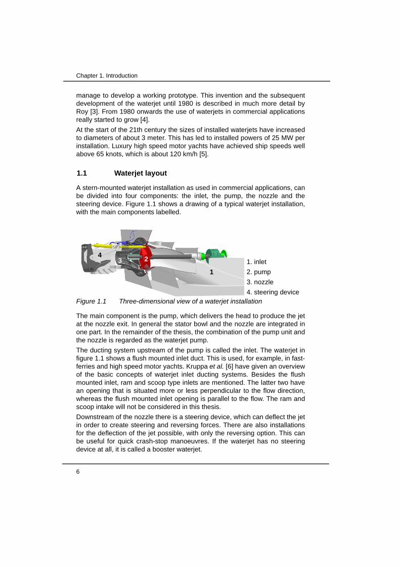
A stern-mounted waterjet installation as used in commercial applications, canbe divided into four components: the inlet, the pump, the nozzle and thesteering device. Figure 1.1 shows a drawing of a typical waterjet installation,with the main components labelled.
The main component is the pump, which delivers the head to produce the jetat the nozzle exit. In general the stator bowl and the nozzle are integrated inone part. In the remainder of the thesis, the combination of the pump unit andthe nozzle is regarded as the waterjet pump.
The ducting system upstream of the pump is called the inlet. The waterjet infigure 1.1 shows a flush mounted inlet duct. This is used, for example, in fast-ferries and high speed motor yachts. Kruppa et al. [6] have given an overviewof the basic concepts of waterjet inlet ducting systems. Besides the flushmounted inlet, ram and scoop type inlets are mentioned. The latter two havean opening that is situated more or less perpendicular to the flow direction,whereas the flush mounted inlet opening is parallel to the flow. The ram andscoop intake will not be considered in this thesis.
Downstream of the nozzle there is a steering device, which can deflect the jetin order to create steering and reversing forces. There are also installationsfor the deflection of the jet possible, with only the reversing option. This canbe useful for quick crash-stop manoeuvres. If the waterjet has no steeringdevice at all, it is called a booster waterjet.
1
234
1. inlet
2. pump
3. nozzle
4. steering deviceFigure 1.1 Three-dimensional view of a waterjet installation
1.2 Relation of waterjet propulsion system to other turbo machinery
Numerical analysis of a waterjet propulsion system 7
1.2 Relation of waterjet propulsion system to other turbomachinery
If the very early 17th century developments are neglected, waterjetpropulsion is relatively new. For further development of the installation it maybe useful to look at related engineering applications. Figure 1.2 shows a boxwith eight different types of apparatus. The three faces which are connectedto the waterjet share a common property.
The front face is formed by four installations which are designed to producethrust. This group contains, besides the waterjet, the ship propeller and thetwo main aeroplane propulsion systems. Any thrust production by theinstallations at the back face (mixed-flow pump, compressor, ventilator andmixer) is an undesirable side effect.
If history is reviewed an interesting parallel can be recognised. In aerospacethe propeller has been replaced by the jet engine, which was necessary toreach higher speeds. Application of waterjets in marine industry shows asimilar trend where the waterjet propelled vessels reach higher speeds.
Many relations which describe the principles of waterjet propulsion aredirectly derived from propeller theory, with the same nomenclature. This canlead to misunderstandings, if the same waterjet is described as a mixed-flowpump, with the accompanying pump nomenclature. For example, often Q isused for torque in propeller theory and for flow rate in pump theory.
The two side planes of the box show the difference in type of flow. The leftside is formed by external flow machines and the right side by internal flowmachines. Transmission of the forces in an external flow machine can only bedone through the shaft. Internal flow machines can also transfer forcesthrough the surrounding structure.
The top plane of the box shows four installations which operate in water,whereas the applications on the bottom plane operate in air. So here the fluidis the distinguishing factor. Cavitation is a typical problem for installationsoperating in water. Another important fluid property of water is its very lowcompressibility. Both phenomena can be important in the selection ofnumerical solution methods. Numerical methods used for the analysis ofcompressors and other flow machinery often require a certain amount ofcompressibility, what makes these methods less suitable for the analysis of awaterjet propulsion system.
The box model will be used to relate the occurring phenomena in a waterjetinstallation to known ones in other machines, like the ship propeller, theaeroplane jet engine and the mixed-flow pump.
A ship propeller seems to be the most logical connection to a waterjet for adescription of the propulsion system. Typical parameters used in propeller

8
Chapter 1. Introduction
theory are the thrust loading coefficient and the cavitation number [7]. Theseparameters can be employed to describe the performance of a waterjet aswell. Moreover the concept of wake fraction, which represents the differencebetween the free stream advance speed and actual inflow velocity, can beused to account for the effect of the hull boundary layer ingestion.
It is well-known that the inflow velocity distribution to the waterjet impeller isstrongly non-uniform. This is similar to the wake field of a ship propeller. Dueto this wake field the loading of a propeller blade fluctuates during arevolution. This results in fluctuations of the pressure distribution on theblades and in a radial force on the shaft. These phenomena will also bepresent in a waterjet. Therefore the choice of a propeller as a starting pointfor the analysis of a waterjet installation seems to be logical. However, thereis a very important difference between a propeller and a waterjet installation.A propeller is an external flow machine whereas the waterjet installation ismainly an internal flow system. The thrust of a propeller will always be guidedthrough the shaft into the ship. In a waterjet installation the forces can betransferred to the vessel via the shaft and via the ship structure. In fact it ispossible to have a higher thrust acting on the shaft than the net thrust of theinstallation [8]. In that case a negative force will work on the transom sternand the inlet ducting.
Figure 1.2 Box model of connections of waterjet to other types of turbomachinery

1.2 Relation of waterjet propulsion system to other turbo machinery
Numerical analysis of a waterjet propulsion system 9
Because the ship propeller operates as an external flow machine, the shipspeed can be used as a governing parameter for the operating point. In non-dimensional notation it is called advance ratio (see for example [10], [10]):
(1.1)
where vship is the ship (or advance) speed, n the shaft speed and D thediameter of the propeller.
The working point of the waterjet installation is based on the volume flow rateQ through the system. In this system the pump head curve matches thesystem resistance curve, which is based on the required head to produce thejet velocity and the head to overcome the hydraulic losses. The influence ofship speed on the operating condition is small.
As a consequence, the available set of propeller equations cannot be usedfor a good description of the waterjet propulsion system.
The theory of aeroplane jet engines may provide the missing equations todescribe the performance of a waterjet system. A turbojet engine is a thrustproducing internal turbomachine, just like the waterjet. The turbojet enginecan be divided into five major components: intake, compressor, combustionchamber, turbine and nozzle (see for example [11]). These componentsinclude the power generating part of the jet engine, i.e. the compressor isdriven by the turbine. In a waterjet a separate diesel engine or gas turbine isneeded to supply the required power to the shaft.
Net thrust of a turbojet engine is based on the change of momentum:
(1.2)
where is the mass flow through the system, vout the jet velocity leaving theengine and vin the velocity of the air entering the intake, which is equal andopposite to the forward speed of the aircraft. Strictly spoken the mass flow inthe system increases due to the addition of fuel, but this increase in massflow is negligible. According to equation (1.2), the thrust of a waterjet systemis directly related to the volume flow rate, since the flow is incompressible:
.
The definition of the propulsive efficiency of a turbojet engine can be found inliterature [11]:
(1.3)
which is often denoted as Froude efficiency. The ratio between intake andnozzle velocity is called nozzle velocity ratio (NVR = vout/vin). At zero speed
Jvship
nD-------------=
F m· vout vin–( )=
m·
m· ρQ=
ηp
F vin⋅Pshaft--------------- 2
1 vout vin⁄( )+------------------------------------= =

10
Chapter 1. Introduction
the NVR becomes infinite, therefore the reciprocal value is used in literaturefor waterjets; this is known as jet velocity ratio µ [12].
Although the working principle of the aeroplane jet engine and the waterjetseem to be similar, it should be kept into mind that cavitation and non-uniforminflow, two important issues in waterjet propulsion, are not dealt with injetengine research.
The third type of turbomachinery which may provide part of the basic theoryto describe system performance is a mixed-flow pump. At first sight this is abit strange, because normally the axial thrust in pump operation is notexploited. Nevertheless, the head curve of the pump and the systemresistance curve provide sufficient information to determine the volume flowrate Q through the system. To get a first estimation of the thrust of thesystem, only the average velocity of the ingested flow and the dimension ofthe nozzle diameter have to be known.
1.3 Aim of the analysis
In this thesis a detailed analysis of a waterjet propulsion system is made.Results of Computational Fluid Dynamics (CFD) calculations are used to getan impression of the flow phenomena occurring in such systems and toquantify system parameters, such as flow rate, torque and thrust. With theapplication of a numerical method some flow features are easier to determinethan in a model scale test. Typical complicating factors in the analysis ofwaterjets are the boundary layer ingestion and the non-uniform velocitydistribution just upstream of the pump. Unfortunately, both the boundary layeringestion as well as the non-uniformity of the velocity distribution areinevitable in commercial waterjet propulsion systems with a flush type of inlet.The major problem of the impeller inlet velocity distribution is the largevariation of the velocity in circumferential direction. This will give rise to ablade loading, which varies strongly with time. This may lead to a decrease insystem performance, like a reduced efficiency, a deterioration in cavitationbehaviour and an increase of forces acting on the impeller. Thesephenomena will increase the noise and vibrations in the installation.
The aim of the analysis presented in this thesis is (i) to quantify the effects ofthe non-uniform inflow to the mixed-flow pump and the resulting non-stationary flow in the pump on the system performance and (ii) to quantify theforces on the complete waterjet installation in both axial and vertical direction.The currently used theory to determine system performance includes someassumptions about the influence of the pressure distribution on thestreamtube of the ingested water. These assumptions will be reviewed tocheck their validity.

1.4 Outline of this thesis
Numerical analysis of a waterjet propulsion system 11
1.4 Outline of this thesis
In chapter 2 the conventional theory of waterjet propulsion systems will bediscussed in detail. This will give insight in the governing parameters of thetotal propulsion system. Some connections will be made with standardpropeller theory to show the similarities and the differences. Some of theunderlying assumptions made will be discussed to enable assessment ofthese assumptions later on. The analysis also reveals the basic principles ofwaterjet selection which is suitable for most of the current applications.
Values for pump parameters in literature are based on uniform inflow.However, it is well-known that a waterjet impeller has to operate in a non-uniform inflow velocity field. The nature of the velocity distribution will bediscussed in chapter 3. Results of measurements will be shown to give animpression of the level of non-uniformity. It is concluded that the typical non-uniform velocity distributions are inevitable in waterjet installations with flushmounted inlets, based on an analysis of the development of the non-uniformity in the duct upstream of the impeller.
Chapter 4 deals with the choice of a mathematical method to analyse the flowthrough the system. An evaluation of several methods, such as potential flow,Euler and RANS, will be presented. An important requirement is the capabilityto capture the effects of the non-uniform inflow to the pump.
The chosen method for the calculation of the flow through a waterjet inlet willbe validated with available experimental data in chapter 5. In thesecalculations, the mass flow rate is prescribed as a boundary condition, sincethe pump is not included in the model. The results of the numerical analysisof the inlet will also be used to evaluate the shape of the streamtubeupstream of the inlet duct. Determination of this streamtube enables a moredetailed analysis of the momentum distribution of the ingested water.
Chapter 6 will deal with the numerical analysis of the non-stationary flowthrough the mixed-flow pump. Results of calculations are compared withmodel scale measurements of the pump performance. Transient calculationswith both uniform and non-uniform velocity distributions will show thepresence of fluctuating radial forces. These forces are strongly related to thelevel of non-uniformity in the flow.
Chapter 7 will show the results of the analysis of a complete full scalewaterjet propulsion system. Overall performance indicators, like volume flow,thrust and power, will be analysed. Comparisons are made with performanceprediction software of Wärtsilä Propulsion Netherlands (WPNL). A moredetailed analysis of the streamtube will reveal some new insights into theforces acting on the installation in vertical direction.
Finally, the conclusions of the present research will be presented in chapter8.

12
Chapter 1. Introduction
1.5 Nomenclature
D propeller diameter m
F thrust N
J advance ratio of propeller (= vship/nD) -
mass flow rate kg/s
n rotational speed 1/s
NVR nozzle velocity ratio (NVR = vout/vin) -
Pshaft shaft power W
Q volume flow rate m3/s
vship advance velocity of propeller m/s
vin advance velocity of jet-engine m/s
vout jet velocity of jet-engine m/s
Greek symbols
ηp propulsive efficiency -
µ jet velocity ratio (= 1 / NVR) -
ρ fluid density kg/m3
1.6 References
[1] Voulon, S., ‘Waterjets and Propellers, Propulsors for the future’, Pro-ceedings SATEC’96 conference, Genoa, Italy, 1995
[2] Ramseye, David, ‘Manufacture of Saltpetre, Raising Water, PropellingVessels, &c.’, English patent no. 50, 1630
[3] Roy, S.M., ‘The evolution of the modern waterjet marine propulsionunit’, Proceedings RINA Waterjet Propulsion conference, London,1994
[4] Warren, N.F., & Sims, N.,’Waterjet propulsion, a shipbuilder’s view’,Proceedings RINA Waterjet Propulsion conference, London, 1994
[5] Bulten, N. & Verbeek, R.,’Design of optimal inlet duct geometry basedon operational profile’, Proceedings FAST2003 conference Vol I, ses-sion A2, pp 35-40, Ischia, Italy, 2003
[6] Kruppa, C., Brandt, H., Östergaard, C., ‘Wasserstrahlantriebe fürHochgeschwindigkeitsfahrzeuge’, Jahrbuch der STG 62, Band 1968,Nov., pp. 228-258, 1968
[7] Terwisga, T.J.C. van,’Waterjet hull interaction’, PhD thesis, Delft, 1996
m·
1.6 References
Numerical analysis of a waterjet propulsion system 13
[8] Verbeek, R.,’Waterjet forces and transom flange design’, RINA waterjetpropulsion conference, London, 1994
[9] Newman, J.N., ‘Marine hydrodynamics’, MIT press, 1977
[10] Lewis, E.V., ‘Principles of naval architecture’, Volume II, Society ofNaval Architects and Marine Engineers, Jersey City, 1998
[11] Cohen, H., Rogers, G.F.C., Saravanamuttoo, H.I.H., ‘Gas turbine the-ory’, Longman Group, London, 1972
[12] Verbeek, R.,’Application of waterjets in high-speed craft’, in Hydrody-namics: Computations, Model Tests and Reality, H.J.J. van den Boom(Editor) Elsevier Science Publication, 1992

14
Chapter 1. Introduction

Numerical analysis of a waterjet propulsion system 15
Chapter 2 Waterjet propulsion theory
In this chapter the basic principles of waterjet propulsion will be discussed.The equations of the waterjet theory will be based on standard nomenclatureused in the description of pump performance. Where possible, equivalentnomenclature of commonly used propeller theory will be mentioned as areference.
In the first section some specific velocities, as used in waterjet theory, will bedefined. These definitions form the basis for the remainder of the chapter. Inthe second section, the generally applied standard parameters are defined,which are used to describe the overall pump performance.
In the commonly used waterjet propulsion theory, equations for the derivationof thrust of a waterjet propulsion system are based on open propeller theory.The transition from open propellers to waterjets will be reviewed in detail, inorder to reveal possible deficiencies in the waterjet theory.
The equations for the waterjet thrust can be coupled to the required pumphead and flow rate. This will be discussed in section 2.4. It will be shown thata certain thrust can be achieved with different combinations of flow rate andpump head. Determination of the optimal combination of flow rate and pumphead is obtained with the aid of the overall propulsive efficiency. This willresult in the design operating point of the pump in the waterjet installation.
In some conditions, the optimal pump operating point can not be reached dueto severe cavitation in the pump. This limitation in the optimization processwill be discussed in section 2.5.1.

16
Chapter 2. Waterjet propulsion theory
In the selection of a waterjet installation for ship propulsion the weight of theinstallation is an important issue. To minimize the weight of the system, thesize of the waterjets is selected as small as possible. The shaft speed of thepump is then maximised. It will be shown that for a given available power theminimum required pump size depends on the ship speed. The availablepower is governed by the installed diesel engine or gasturbine. This dictatesthe selection procedure to a large extent.
2.1 Characteristic velocities in a waterjet system
In the equations for pump performance and thrust, use is made of somespecific velocities. Four main velocities are distinguished and will be usedthroughout this thesis:
1. ship speed (vship)2. mass averaged ingested velocity at duct inlet (vin)
3. averaged axial inflow velocity at the pump entrance (vpump)
4. averaged outlet velocity at the nozzle (vout)
Figure 2.1 shows a sketch of a waterjet installation with the four velocitiesindicated. A non-uniform velocity distribution is sketched to indicate thedevelopment of the boundary layer along the hull surface, upstream of theinlet. This figure is also used to give an impression of the dividing streamline.By definition there will be no mass flow across this line. In three dimensions,this line is extended to a dividing streamtube. The curved part of the inlet,where the streamline ends, is denoted as inlet lip or cutwater.
The inlet velocity is determined at a cross-flow plane just upstream of thewaterjet inlet, where the influence of the waterjet is not yet noticeable. Theingested velocity distribution is mass-averaged over the cross-sectionalshape of the streamtube to find the actual inlet velocity vin:
(2.1)
vout
vship
vin
vpump
Figure 2.1 Characteristic velocities in waterjet propulsion system
z
x
l
vin1Q---- v z( )vn Ad
A∫=

2.1 Characteristic velocities in a waterjet system
Numerical analysis of a waterjet propulsion system 17
where v(z) is the velocity distribution in the boundary layer.
The four velocities are related by three parameters; wake fraction, inletvelocity ratio and jet velocity ratio. These three parameters are discussed indetail in this section.
2.1.1 Wake fraction
The water that is ingested into the waterjet inlet channel partly originates fromthe hull’s boundary layer. The mass averaged velocity of the ingested water(vin) is lower than the ship speed due to this boundary layer. The velocitydeficit is expressed as the momentum wake fraction (w), which is defined as:
(2.2)
Calculation of the wake fraction is rather complex, since the cross-sectionalshape of the streamtube is not known a priori. Experiments have revealedthat the cross-section of the streamtube has a semi-elliptical shape under thehull [1]. This is often simplified by a rectangular box with a width of 1.3 timesthe pump diameter. Some comparisons have been made with experimentalresults [2], [3] and it is concluded that the resulting value for the wake fractioncan be determined within acceptable limits, if the rectangular boxapproximation is used.
For a given volume flow rate through the waterjet the height of the box can becalculated once the velocity distribution in the boundary layer is known.Standard theory for a flat plate boundary layer, as described in severaltextbooks ([4], [5]) can be used to get a first indication of the velocitydistribution. It is convenient to use a power law velocity profile for theboundary layer velocity distribution:
(2.3)
where v denotes the local velocity in the boundary layer at a distance znormal to the wall, the undisturbed velocity, δ the local boundary layer
thickness and n the power law index.
Besides the thickness of the boundary layer δ there are also derivedquantities like the displacement thickness δ1 and momentum thickness δ2 ofthe boundary layer.
w 1vin
vship-------------–=
vU∞------- z
δ---
1n---
=
U∞

18
Chapter 2. Waterjet propulsion theory
The momentum thickness can be related to the wall friction coefficient cf(l) fora flat plate:
(2.4)
where l is the wetted length. This relation gives the frictional drag of the flatplate in terms of the development of the boundary layer.
Substitution of the power law velocity distribution in the definitions of theboundary displacement thickness δ1, the momentum thickness δ2 and theenergy thickness δ3 results in a set of the following relations:
(2.5)
(2.6)
(2.7)
Combination of equations (2.4) and (2.6) gives an expression for the frictioncoefficient cf(l) as function of the boundary layer thickness δ(l) and the powerlaw exponent n. For turbulent flow a value of n = 7 is often used. With aid ofthe analysis of developed turbulent pipe flow, an expression for the flat plateboundary layer thickness is derived:
(2.8)
where Rel is the Reynolds number based on the wetted length. The wallfriction coefficient for n=7 becomes:
(2.9)
Comparison with experimental data shows good agreement for Reynolds
numbers between 5x10⁵ and 107 (see [4]).
In general, full scale waterjet installations operate at Reynolds numbers of
about 109, which is 2 orders of magnitude larger. The wall friction coefficientfor a flat plate cannot be based on equation (2.9) at these high Reynoldsnumbers. Several logaritmic equations for the flat plate wall friction coefficientare defined for high Reynolds numbers. A typical example is the ITTC’57
cf l( )τw
12---ρU∞
2------------------≡ 2
ld
dδ2=
δ1δ
n 1+-------------=
δ2δn
n 1+( ) n 2+( )------------------------------------=
δ32δn
n 1+( ) n 3+( )------------------------------------=
δn 7=
0.370 l Rel1 5⁄–⋅ ⋅=
cf l( ) 0.0576 Rel1 5⁄–⋅=

2.1 Characteristic velocities in a waterjet system
Numerical analysis of a waterjet propulsion system 19
friction line, which is commonly used to extrapolate the viscous resistancecomponent of a model scale ship to full scale dimensions.
The logaritmic friction line gives the wall friction coefficient as function ofReynolds number. Based on equations (2.4) and (2.6), there is a relationbetween friction coefficient cf(l), boundary layer thickness δ(l) and power lawexponent n. The actual power law exponent n is determined from velocityprofile measurements by Wieghart. Results of measurements at differentReynolds numbers are presented in Schlichting [4]. For a certain Reynoldsnumber, the corresponding boundary layer thickness can be calculated oncethe wall friction coefficient cf(l) and the power law exponent n are established.
Full scale measurements of the hull boundary layer velocity distribution arepresented by Svensson [7]. Velocity profiles are measured on two differentvessels and at different ship speeds. This results in a large variation ofReynolds numbers. A reasonable fit of a power law profile with n = 9 and themeasured values is found. The equation for the boundary layer thickness, asgiven in equation (2.8), is modified for n = 9:
(2.10)
It can be noticed that both the constant as well as the power of the Reynoldsnumber have to be changed when the value of n is changed. This is inaccordance with measurements of Wieghardt (see [4]). Adjustment of thesevalues should result in the right boundary layer thickness and in an accurateprediction of the velocity profile and the wall friction. For Reynolds numbers of
order 109 the power law exponent becomes 10 to 11.
With known boundary layer thickness and volume flow through the pump, theaverage incoming velocity and thus the wake fraction can be calculated. Atypical value for the wake fraction w is 0.10 to 0.14 for a fast ferry.
The accuracy of the rectangular box approximation will be reviewed inchapter 5 when CFD calculations of the flow through the waterjet inlet ductare discussed. With the numerical method it is possible to visualize the actualshape of the streamtube and determine the mass-averaged velocity bynumerical integration. This numerical method is based on the computedshape of the streamtube, whereas the determination of the wake fraction inexperiments is based on an approximated shape of the streamtube.Consequently, the wake fraction obtained from the numerical results is moreaccurate than the one obtained from experimental data.
δ n 9= 0.270 l Rel1– 6⁄⋅ ⋅=

20
Chapter 2. Waterjet propulsion theory
2.1.2 Inlet velocity ratio
The averaged axial inflow velocity of the pump is denoted by vpump. Thisvelocity can be written as:
(2.11)
where Q is the volume flow through the pump and Dinlet the diameter at thesuction side of the pump. This velocity is an important parameter to describethe flow phenomena in the inlet, where the speed is changed from the shipspeed to the pump velocity. The pump velocity is related to the ship speedthrough the Inlet Velocity Ratio (IVR):
(2.12)
At normal operating condition, IVR will be around 1.3 to 1.8. The reciprocal ofequation (2.12) is used in literature as well ([2], [8]) and used by the ITTC; thisresults in values of this quantity, at operating conditions below 1 and a valueof infinite for zero ship speed. Use of the definition in equation (2.12) ispreferred since the operating range is bounded between 0 and about 2.5.
IVR is used to denote the flow conditions in the waterjet inlet duct. Atrelatively low ship speed, e.g. during manoeuvring in harbour, IVR will besmaller than 1. This means that the flow is accelerated upon entering the inletduct. In this condition the stagnation point of the dividing streamline is locatedat the hull side of the inlet lip (or cutwater). This might lead to cavitation and/or separation in the inlet at the upper side of the lip. Figure 2.2 shows asketch of the flow phenomena at low IVR condition.
If the vessel sails at design speed, the inlet flow phenomena are quitedifferent. As mentioned, the design IVR will be around 1.3 to 1.8. IVR values
vpumpQ
π4---Dinlet
2------------------=
IVRvship
vpump----------------=
Increased risk for
Figure 2.2 Flow phenomena at low IVR
cavitation and/or separation

2.1 Characteristic velocities in a waterjet system
Numerical analysis of a waterjet propulsion system 21
of more than 2.0 are known for high speed motor yachts (>60 knots). Thisimplies a significant deceleration of the flow in the inlet. In this condition thestagnation point is located at the inlet side of the cutwater. The criticallocation for cavitation is located at the hull side of the lip for this condition.The deceleration of the flow in the inlet duct leads to an adverse pressuregradient in the inlet. If this pressure gradient becomes too large, flowseparation is likely to occur at the top side of the inlet. The possible flowphenomena at high IVR are sketched in figure 2.3.
Whether or not cavitation or separation really occurs in a practical situation,strongly depends on the actual geometry of the inlet duct. With a good inletdesign cavitation and separation free operation is possible up to about 44knots [9], which is a commonly used design speed for fast ferries.
It should be kept in mind, that an inlet has to be designed to cope with the lowIVR and the design IVR condition, because each vessel has to start from zeroship speed.
2.1.3 Jet velocity ratio
The velocity vout at the outlet of the waterjet nozzle, is related to the volumeflow through the pump and the diameter of the nozzle as:
(2.13)
The outlet velocity is related to the incoming velocity by the jet velocity ratio µ:according to [10]:
(2.14)
Increased risk of cavitation
Increased risk of separation
Figure 2.3 Flow phenomena at high IVR
voutQ
π4---Dnozzle
2------------------------=
µvin
vout----------=

22
Chapter 2. Waterjet propulsion theory
The importance of the parameter µ will be shown in section 2.5, where theoverall propulsive efficiency of the waterjet system is derived. It will be shownthat typical values are in the range of 0.5 to 0.7.
2.1.4 Summary
In this section four velocities are introduced; vship, vin, vpump and vout. Therelations between these velocities are defined by three ratios: wake fractionw, inlet velocity ratio IVR and nozzle velocity ratio µ. The theory of waterjetpropulsion will be based on these velocities and ratios.
2.2 General pump theory
In this section a short overview of the standard pump theory is given in orderto introduce a set of parameters to describe the pump performance. Thistheory can be found in many textbooks about centrifugal pumps, see forexample [11], [12].
2.2.1 Dimensionless performance parameters
Performance of a pump can be expressed in terms of a set of non-dimensional parameters. The performance is expressed in terms of flow rate,head and cavitation behaviour. In dimensionless form, the flow rate throughthe pump is given as the flow coefficient ϕ:
(2.15)
where Q is the flow rate in m3/s, Ω the speed of the impeller in rad/s and Dthe impeller diameter in m. The head coefficient ψ of a pump is defined as:
(2.16)
where H is the head in m. It can be shown that geometrically similar pumpshave equal values for flow and head coefficient. This forms the basis of theso-called similarity method. If the performance of a pump for a certain sizeand shaft speed is known, equations (2.15) and (2.16) can be used to predictthe performance for different sizes and shaft speeds. Elimination of thediameter D from equations (2.15) and (2.16) results in:
(2.17)
ϕ Q
ΩD3
------------≡
ψ gH
ΩD( )2-----------------≡
1ΩQ
1 2⁄
gH( )3 4⁄--------------------- ψ3 4⁄
ϕ1 2⁄------------⋅=

2.2 General pump theory
Numerical analysis of a waterjet propulsion system 23
which leads to the definition of the specific speed of:
(2.18)
where Ω is the speed of the impeller in rad/s, Q the flow rate in m3/s and Hthe head in m. It is also found that the similarity method implies thatgeometrically similar pumps have equal values of specific speed:
(2.19)
The value of the specific speed of a specific pump gives a good indication ofits type: typical axial flow pumps have a specific speed above 2.4, whereasradial flow pumps have low values of the specific speed (typically below 1.0).Mixed-flow pumps have intermediate values for the specific speed.
Pump efficiency ηpump is defined as the ratio between the hydraulic powerPhydr, which is the product of flow rate and pressure rise, and the requiredshaft power Pshaft.
(2.20)
where Tq is the shaft torque. The required shaft power can be expressed in a
non-dimensional specific power P*:
(2.21)
The specific power is related to the flow coefficient, head coefficient andpump efficiency. Combination of equations (2.15), (2.16) and (2.20) yields:
(2.22)
Strictly speaking, similarity of performance is only valid in cases of bothgeometrically and dynamically similar internal flows. In this analysis viscosityis not taken into account. Since hydraulic losses do scale differently,additional empirical relations are used to predict the effect of these losses onpump efficiency and specific power.
nωΩ Q
g H⋅( )3 4⁄-------------------------≡
nωϕ1 2⁄
ψ3 4⁄------------=
ηpump
Phydr
Pshaft---------------- ρgHQ
ΩTq----------------= =
P* Pshaft
ρΩ3D
5------------------=
P* ϕψ
ηpump----------------=

24
Chapter 2. Waterjet propulsion theory
2.2.2 Pump geometry parameters
It is shown in the preceding section, that the specific speed is found from theexpressions for flow coefficient and the head coefficient, when the diameter iseliminated. In a similar way, the specific diameter δ is found, if the rotationalspeed Ω is eliminated:
(2.23)
so that:
(2.24)
and:
(2.25)
The specific speed and specific diameter are based on the same twoparameters, namely ϕ and ψ. The relation between the two is represented inthe so called Cordier-diagram [14], which is based on experience from actualpumps. Waterjet pump designs may deviate from this empirical rule forconventional pumps due to the difference in functionality as outlined inchapter 1.
The basic geometry of the impeller of conventional centrifugal pumps isstrongly related to the specific speed of a pump, however. The largesimilarities in pump geometry lead to comparable efficiencies for differentpumps with the same specific speed. The statistically attainable optimal pumpefficiency can be derived from several published prediction formulas, basedon measured performances. An example of such empirical formula is given in[15]:
(2.26)
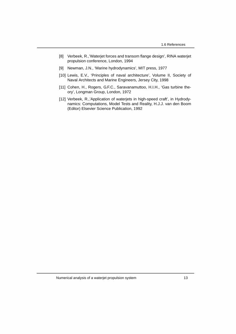
where Qref is set equal to 1 m3/s in order to maintain the non-dimensionalrepresentation. Figure 2.4 shows the expected maximum pump efficiency forthree flow rates. The highest efficiency is found at a specific speed of 1.0.Decrease in efficiency is rather slow when the specific speed is increased tovalues above 1.0. In general, waterjet pumps have a specific speed around2.0-3.0.
1gHD
4
Q2
--------------- ϕ2
ψ------⋅=
δ D gH( )1 4⁄
Q---------------------⋅≡
δψ1 4⁄
ϕ1 2⁄------------=
ηpump 0.950.05
Q Qref⁄3-------------------------– 0.125 nω( )log[ ]2
–=
2.2 General pump theory
Numerical analysis of a waterjet propulsion system 25
Achievable pump efficiencies around 90% for large pumps seem to be areasonable estimate. This value will be used in the remainder of this chapterfor estimates of the overall waterjet efficiency.
2.2.3 Cavitation parameters
For cavitation free operation the pump requires a certain available pressureat the inlet, or suction side. This is denoted with the inception net positivesuction head (NPSHi), which is a pressure expressed in meters watercolumn. In general, pump operation is still possible beyond the cavitationinception level, i.e. for lower NPSH levels. Therefore the criterion for the inletsuction head is based on a certain loss of pump performance (for example 1or 3% head loss or a certain percentage of pump efficiency decrease, see[16]). Based on the choice for the admissible head loss, a required NPSH isdefined.
The required net positive suction head (NPSHR) can be made non-dimensional in a similar way as the head to form the suction coefficient κ:
(2.27)
Another, well-known method to present the NPSH in dimensionlessrepresentation is the Thoma number, defined as:
(2.28)
50%
55%
60%
65%
70%
75%
80%
85%
90%
95%
100%
0 0.5 1 1.5 2 2.5 3 3.5 4 4.5 5
Q= 0.1 m3/s
Q= 1.0 m3/s
Q= 10 m3/s
Figure 2.4 Maximum pump efficiency as function of specific speed, based on equation (2.26).
η pum
p [−
]
Pump specific speed Nω [−]
κgNPSHR
ΩD( )2-------------------------=
σNPSHR
H---------------------=

26
Chapter 2. Waterjet propulsion theory
The non-dimensional parameters are related by the head coefficient.
The required NPSH can also be related to the flow rate and the rotationalspeed of the impeller, similar to the pump specific speed. This gives thesuction specific speed of the pump nωs, defined as:
(2.29)
The suction specific speed of a pump is more or less constant for all pumptypes. Values of about 4.0 are common in commercial pumps [14-17]. Inorder to create some extra margin to accommodate cavitation, a design valueof 3.5 for a waterjet impeller is adopted.
2.2.4 Correlation with propeller performance parameters
The flow coefficient ϕ of a pump can be related to the propeller advance ratioJ (as given in eqn. (1.1)) with substitution of equations (2.11) and (2.12):
(2.30)
This relation shows the fundamental difference between an open propellerand a waterjet installation, where in the waterjet IVR is introduced as anadditional parameter. This parameter is needed because of the principle ofinternal flow of the pump compared to the external flow of the propeller.
In a similar way, the non-dimensional head can be related to the thrustcoefficient of an open propeller. For a propeller the thrust coefficient isdefined as [18]:
(2.31)
The head H of a pump is related to the total pressure increase generated bythe impeller according to:
(2.32)
In actuator disk theory the production of thrust of an open propeller equals theproduct of the pressure rise and the cross-sectional area of the propeller:
(2.33)
It is assumed that the static pressure rise is equal to the total pressure rise,due to the infinitesimal thickness of the actuator disk. This results in a relation
nωsΩ Q
g NPSHR⋅( )3 4⁄------------------------------------------=
ϕπvpump
4ΩD-------------------- J
8IVR--------------= =
KTT
ρn2D
4-----------------=
∆ptot ρgH=
T ∆p Aprop⋅=

2.3 Thrust
Numerical analysis of a waterjet propulsion system 27
between the head coefficient ψ of a pump and the thrust coefficient KT of apropeller:
(2.34)
It is concluded that the Q-H curves of a pump are equivalent to the J-KTcurves of an open propeller. The main difference is caused by the used inflowvelocity.
2.3 Thrust
2.3.1 General thrust equation
The purpose of a propulsion installation is to produce thrust to propel avessel. Water is accelerated in the installation, which results in a reactionforce on the ship structure. The thrust can be derived from the momentumbalance for an incompressible fluid [5]:
(2.35)
The momentum balance states that the sum of all surface forces Fs and allbody forces Fb acting on the spatially fixed control volume V equals the rateof change of momentum in the control volume with surface A. The surfaceforce is defined as:
(2.36)
where p is the static pressure, I the unit tensor and σ the viscous stresstensor.
In the remainder of this section the steady flow situation will be analysed. Asa consequence, the first term on the right hand side of equation (2.35)vanishes. Moreover, the body forces, like gravity, acting on the fluid will beneglected.
In the following subsections the momentum balance will be derived for bothan open propeller and a waterjet.
ψ ∆p( ) ρ⁄
4π2n
2D
2------------------------
KT
π3-------= =
F Fs Fb+t∂
∂ vρ V v
A∫+d
V∫ ρv Ad⋅= =
Fs p– I σ+( ) Ad⋅A∫=

28
Chapter 2. Waterjet propulsion theory
2.3.2 Open propeller thrust
An expression for the thrust of an open propeller is determined with equation(2.35) [6]. The propeller is treated as an actuator disk, which is a singularitymodelled by a body force acting over an infinitesimal thin disk. The controlvolume consists of the streamtube of fluid which passes through the propellerplane area. Figure 2.5 shows a sketch of the control volume of an openpropeller with the nomenclature of the velocities.
Evaluation of the momentum balance is split in two parts; the contribution ofthe momentum fluxes and the contribution of the surface forces. Thecontributions of the momentum fluxes in x-direction result in a net momentumflux component in x-direction of:
(2.37)
This can be rewritten, with aid of the continuity condition, as:
(2.38)
The contributions of the surface forces in x-direction are defined as:
(2.39)
It is assumed that the pressure at the inlet (far upstream) and at the outlet (fardownstream) is equal to the ambient pressure . Moreover, the contribution
of the viscous forces is neglected on the inlet and outlet area as well as on
vinvout
vprop
ptube
Figure 2.5 Control volume for the momentum balance applied to an propeller within a streamtube
Ain
Aout
Atubez
xp p∞=
p p∞=
φmx ρvout2
Aout ρvin2
Ain–=
φmx ρvpropAprop vout vin–( )=
Fx Tprop– p p∞–( ) Ad
Ain
∫ p p∞–( ) Ad
Aout
∫+– p p∞–( )x Ad⋅Atube
∫+=
p∞

2.3 Thrust
Numerical analysis of a waterjet propulsion system 29
the streamtube surface. Combination of equations (2.38) and (2.39) gives thefinal thrust equation for an open propeller, based on the momentum balance:
(2.40)
where Aprop is the cross-sectional area of the propeller plane, x the unitvector in x-direction and Atube the streamtube surface. The contribution of thepressure acting on the streamtube to the thrust vanishes, based on theparadox of d’Alembert, if the streamlines are aligned in x-direction farupstream and downstream.
If Bernoulli’s theorem is applied along the streamlines in the part of thecontrol volume upstream and downstream of the propeller, a second relationfor the propeller thrust is found:
(2.41)
Combination of the momentum balance and Bernoulli’s law, leads to a simplerelation between the inlet and outlet velocity and the volume flow through thepropeller disk (see [18]):
(2.42)
It can be seen that the velocity through the disk is the average of theupstream and downstream velocities. The difference between the velocitythrough the disk and the incoming velocity is called the induced velocity vind.
Thrust loading coefficient
Loading of an open propeller is often expressed by the propeller loadingcoefficient, defined as [18]:
(2.43)
where Aprop is the cross-sectional area of the propeller disk, based on thepropeller diameter. The propeller loading coefficient can be expressed interms of the ratios as defined in section 2.1. Substitution of equation (2.41),with the inflow velocity equal to the ship speed, i.e. vin=vship, yields:
Tprop ρApropvprop vout vin–( ) p p∞–( )x Ad⋅Atube
∫–=
Tprop ∆p Aprop⋅ ρAprop12--- vout
2vin
2–( )⋅= =
vprop12--- vin vout+( ) vin vind+= =
CTprop
Tprop
12---ρvship
2Aprop
------------------------------------=

30
Chapter 2. Waterjet propulsion theory
(2.44)
With µ<1 the propeller loading coefficient is thus directly related to the jetvelocity ratio.
The jet velocity ratio can be related to the IVR, if equation (2.42) is substitutedinto equation (2.12):
(2.45a)
It can be seen that open propellers always operate at IVR values below 1.After rearranging this equation, it is shown that the IVR is equal to Froudeefficiency as given in equation (1.3):
(2.45b)
Although the term IVR is not used in the theory for open propellers, it isalready present as the Froude efficiency.
2.3.3 Waterjet thrust
For the determination of the thrust of a waterjet installation in general thesame approach as for the open propeller is used. The control volume will bebounded by the streamtube surface on one side and the solid wall on theother side. It is assumed that the inlet and exit planes are perpendicular to thex-direction and the hull is parallel to the x-axis. Figure 2.6 shows the controlvolume and the contributing terms to the momentum balance. The forcesacting on the waterjet structure, which are included in this control volume, aredenoted as Twj,tube.
It is noted that the control volume based on the streamtube of the ingestedwater does not take into account the part of the waterjet inlet structure at thehull side near the cutwater lip, which is excluded from the streamtube controlvolume. The thrust or drag on that part of the waterjet structure will bedenoted will Twj,hull. At high IVR conditions a significant part of the cutwatergeometry belongs to the excluded cutwater region. The subdivision of thecomplete waterjet inlet structure into the part, which is included in thestreamtube approach, and the part which is excluded is shown in figure 2.7.
CTprop
12---ρ vout
2vin
2–( )Aprop
12---ρvin
2Aprop
---------------------------------------------------vout
vin----------
21–
1 µ2–
µ2---------------= = =
IVRvin
vprop-------------
2vin
vin vout+------------------------ 2µ
µ 1+-------------= = =
IVR2
11µ---+
------------- 21 vout vin⁄( )+----------------------------------- ηp= = =

2.3 Thrust
Numerical analysis of a waterjet propulsion system 31
The total thrust Twj,all of a waterjet is therefore:
(2.46)
Application of the momentum balance for a waterjet learns that there are twomomentum flux terms that contribute to the force in x-direction; these are thefluxes at the nozzle exit surface Aout and at the plane Ain upstream of theinlet:
vout
vinptube
Figure 2.6 Control volume for a momentum balance on the streamtube of the ingested water of a waterjet installation
z
x
Ain
Atube
Aout
Awj
Ahullp p∞=
p p∞=
all solid wall cells
streamtube solid wall cells
remaining hull cells
Figure 2.7 Subdivision of all solid wall cells of the waterjet installation into group belonging to streamtube control volume (left) and group of remaining cells on hull (right)
Twj all, Twj tube, Twj hull,+=

32
Chapter 2. Waterjet propulsion theory
(2.47)
where vin is the mass averaged inflow velocity. With aid of the continuitycondition, this becomes:
(2.48)
where Q is the flow rate through the waterjet installation. The contributions ofthe surface forces in x-direction are defined as:
(2.49)
Similar to the open propeller, it is assumed that volumetric forces and viscousforces can be neglected, while the pressure levels at the inlet (far upstream)and at the outlet (far downstream) are equal to the ambient pressure .
Effect of the viscous forces is neglected also on these two planes, thoughthere is a non-uniform velocity distribution present at the inlet plane Ain.Contribution of this shear stress force is assumed to be negligible. Withequations (2.48) and (2.49) can be combined to get the expression for thewaterjet thrust in x-direction based on the streamtube momentum balance:
(2.50)
The contribution of the streamtube pressure can not be quantified analytically,since the shape of the streamtube and the pressure distribution are unknown.Even with numerical methods it is a very complex task to determine thisvalue, due to the three-dimensional shape of the streamtube surface and thedependency of the shape on IVR. In chapter 7 the contribution of thestreamtube pressure term will be reviewed in more detail.
The thrust of the complete waterjet installation is found, when equation (2.50)is substituted in equation (2.46), which yields:
(2.51)
The last two terms on the right-hand-side are assumed to be small comparedto the first term, and often neglected in waterjet propulsion literature. The
φmx ρvout2
Aout ρvin2
Ain–=
φmx ρQ vout vin–( )=
Fx Twj tube,– p p∞–( ) Ad
Ain
∫ p p∞–( ) Ad
Aout
∫+– p p∞–( )x Ad⋅Atube
∫+=
p∞
Twj tube, ρQ vout vin–( ) p p∞–( )x Ad⋅Atube
∫–=
Twj all, ρQ vout vin–( ) px Ad⋅Atube
∫– Twj hull,+=

2.3 Thrust
Numerical analysis of a waterjet propulsion system 33
influence of this simplification will be addressed in more detail in chapter 7.The resulting simplified thrust equation for a waterjet becomes [10]:
(2.52)
Despite neglecting the streamtube and hull surface forces, this simplifiedequation can be used to explain the main theory on waterjet propulsion. Thisequation shows the three main parameters of a waterjet propulsion system:the volume flow rate Q through the system, the nozzle exit area Anozzle andthe jet velocity ratio µ.
Thrust loading coefficients
The thrust loading coefficient of a waterjet installation can be based on thenozzle outlet area or the pump inlet area. The thrust loading coefficient basedon nozzle exit area is discussed in [13]. With the nozzle area as referencearea, the relation between jet velocity ratio and the thrust loading coefficientbecomes:
(2.53)
where w is the wake fraction according to equation (2.2). The wake fractionbecomes zero, when the inflow velocity is equal to the ship speed, i.e.vin=vship. This is equivalent with an open water test of a propeller with uniforminflow. The resulting loading coefficient for a waterjet with undisturbed inflowyields:
(2.54)
Comparison with the open propeller thrust loading coefficient (equation(2.44)) reveals a difference between the waterjet and the open propeller. Thisis due to the fact that a waterjet is an internal flow machine. For a waterjet theratio between the inlet and nozzle area is fixed, whereas it is related to thethrust for an open propeller.
The waterjet thrust loading coefficient can also be based on the pump inletdiameter. In this way the dimensions of the complete installation arerecognised more clearly. This approach is more in agreement with the openpropeller thrust loading coefficient, where the propeller diameter is used.
Twj ρQ vout vin–( ) ρQ2
Anozzle------------------- 1 µ–( )= =
CTnozzleT
12---ρvship
2Anozzle
----------------------------------------- 2 1 µ–( ) 1 w–( )2
µ2-------------------------------------------= =
CTnozzle w 0=
2 1 µ–( )
µ2---------------------=

34
Chapter 2. Waterjet propulsion theory
(2.55)
The thrust loading coefficient based on the pump inlet diameter shows thatthe IVR is introduced to describe the system performance. This gives thedesigner of waterjets another optimization option, compared to openpropellers.
2.3.4 Concluding remarks
In a waterjet there is no direct relation between the IVR and µ like there is foran open propeller. Since it is an internal flow machine, part of the thrust canbe transferred to the hull structure via the transom stern and the inlet ducting.On the other hand, it can also appear that the thrust acting on the shaft willexceed the total thrust of the installation [19]. In such condition a negativethrust acts on the transom stern or the inlet ducting. For conventional pumpsthe axial thrust is to be kept as low as possible. Thrust production is notregarded as an important performance indicator, like efficiency and head asfunction of the mass flow.
In case of a waterjet, the thrust can be calculated, if the values for thevelocities vin, vpump and vout are known. These can be related to the massflow for a given geometry of the waterjet installation. This mass flow throughthe system is related to the pump head. In this way the standard pumpperformance characteristics, like head curve, efficiency and cavitationbehaviour, can be used to evaluate the performance of a waterjet installation.
2.4 Pump head
The required head of a waterjet installation will be discussed in this section.The head H of a pump represents the increase of total pressure in a pumpmeasured in meters liquid water column as given in equation (2.32).
The volume flow rate through the system follows from the intersection of therequired system head curve and the pump head curve. The pump head curvedepends on the type of pump used in the waterjet system. In general, mixed-flow pumps have a head-curve with a negative slope in the design point toensure a stable operating point. For lower volume flow rates the slope maybecome zero or even negative. For the sake of simplicity, the pump headcurve, as used in the examples in this section, is assumed to be a linearfunction of flow rate.
CTpumpT
12---ρvship
2Apump
-------------------------------------- 2 1 µ–( ) 1 w–( )2
IVR µ⋅-------------------------------------------= =

2.4 Pump head
Numerical analysis of a waterjet propulsion system 35
The required system head curve can be regarded as a pipe resistance curveof the waterjet installation. The acceleration of the fluid in the nozzle requiresa certain pressure difference. Additional head is required to overcome thehydraulic losses in the inlet and the nozzle. However, the energy of theingested fluid can be used partly, which is beneficial for the headrequirement. Finally, the waterjet nozzle may be positioned above thewaterline, which will require some more pump head. All contributions togethergive the equation for the required system head HR:
(2.56)
where φ is the nozzle loss coefficient, ε the inlet loss coefficient and hj thenozzle elevation above the waterline. The elevation of the nozzle is limited bythe self-priming requirement of the waterjet installation. In general, theelevation hj can be neglected relative to the other contributions in equation(2.56).
Equation (2.56) shows a positive contribution from the incoming velocity,therefore the system performance is coupled to the ship speed. Strictlyspeaking, the average ingested velocity vin should be based on a massaveraged dynamic pressure term:
(2.57)
whereas vin in equation (2.56) is based on the mass averaged velocity asgiven in equation (2.1). The difference between the two methods can beexpressed in the power-law exponent, assumed that the water is ingestedcompletely out of the boundary layer:
(2.58)
The difference between the two methods of averaging is less than 1% for apower-law exponent of n=9. The error will be even smaller if the water isingested from the undisturbed fluid. In general, the introduced deviation iscompensated for in the determination of the loss coefficient.
At constant ship speed, the required system head HR can be approximatedas a quadratic function of the flow rate Q. The slope of this quadratic curvedepends on the nozzle diameter. Figure 2.8 shows an example of a pumphead diagram with a pump head and efficiency curve and two system lines fora constant ship speed and different nozzle sizes. The assumption of constant
HR
vout2
2g---------- 1 φ+( )
vin2
2g------- 1 ε–( )– hj+=
vin˜ 1
Q---- v z( )2
vn Ad
A∫
1 2⁄=
vin˜ 2
vin2
---------- n 2+( )2
n 3+( ) n 1+( )------------------------------------=
36
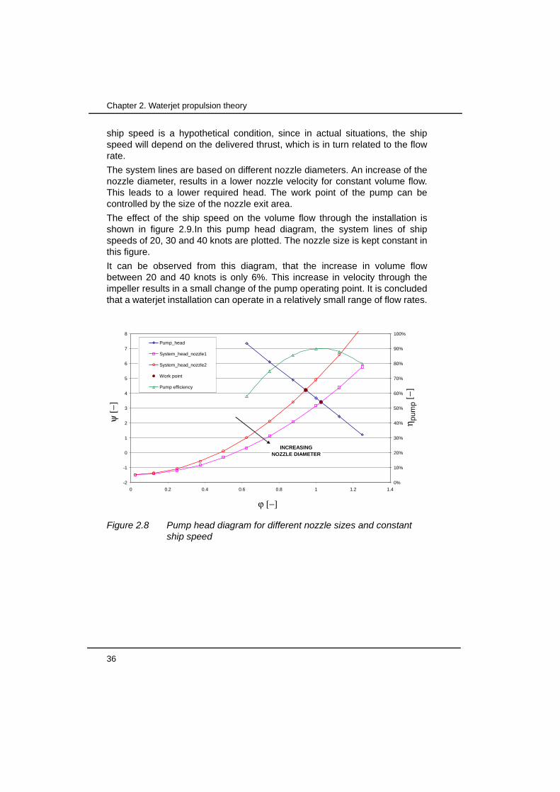
Chapter 2. Waterjet propulsion theory
ship speed is a hypothetical condition, since in actual situations, the shipspeed will depend on the delivered thrust, which is in turn related to the flowrate.
The system lines are based on different nozzle diameters. An increase of thenozzle diameter, results in a lower nozzle velocity for constant volume flow.This leads to a lower required head. The work point of the pump can becontrolled by the size of the nozzle exit area.
The effect of the ship speed on the volume flow through the installation isshown in figure 2.9.In this pump head diagram, the system lines of shipspeeds of 20, 30 and 40 knots are plotted. The nozzle size is kept constant inthis figure.
It can be observed from this diagram, that the increase in volume flowbetween 20 and 40 knots is only 6%. This increase in velocity through theimpeller results in a small change of the pump operating point. It is concludedthat a waterjet installation can operate in a relatively small range of flow rates.
-2
-1
0
1
2
3
4
5
6
7
8
0 0.2 0.4 0.6 0.8 1 1.2 1.40%
10%
20%
30%
40%
50%
60%
70%
80%
90%
100%
Pump_head
System_head_nozzle1
System_head_nozzle2
Work point
Pump efficiency
INCREASINGNOZZLE DIAMETER
Figure 2.8 Pump head diagram for different nozzle sizes and constant ship speed
ψ [−
]
η pum
p [−
]
ϕ [−]

2.5 Overall propulsive efficiency
Numerical analysis of a waterjet propulsion system 37
2.5 Overall propulsive efficiency
This section deals with the influence of the parameter µ on the overallpropulsive efficiency. If the propulsion system is regarded as a black box,then engine power Pshaft is input and thrust T at a certain ship speed isoutput. The overall propulsive efficiency ηd of this black box is then based onthe bare hull resistance Rbh of a vessel [18]:
(2.59)
where Rbh is the bare hull ship resistance and Pshaft the power at the waterjetshaft.
In conventional naval architecture theory, the resistance of a ship with anactive propeller is found to be different from the bare hull resistance. Due tothe action of the propeller, a low pressure region at the rear of the vessel iscreated, which results in an increased drag of the vessel. The differencebetween the bare hull resistance Rbh and the required thrust T at a certainship speed is expressed in terms of the thrust deduction factor t according to:
(2.60)
-2
-1
0
1
2
3
4
5
6
7
8
0 0.2 0.4 0.6 0.8 1 1.2 1.40%
10%
20%
30%
40%
50%
60%
70%
80%
90%
100%
Pump_head
system_head_20 knots
system_head_30 knots
system_head_40 knots
work point
Pump efficiency
INCREASINGSHIP SPEED
Figure 2.9 Pump head diagram for different ship speeds
ψ [−
]
η pum
p [−
]
ϕ [−]
ηd
Rbh vship⋅Pshaft
---------------------------=
Rbh 1 t–( ) T⋅=

38
Chapter 2. Waterjet propulsion theory
For a propeller the thrust deduction factor is always positive, which leads to ahigher ship resistance due to the action of the propeller and therefore ahigher required thrust.
In waterjet propulsion theory, the thrust deduction factor t can be used toaccount for the effects of (i) the neglected surface forces such as the force onthe streamtube and the force on the region aft of the waterjet inlet and (ii) achange in the pressure distribution along the hull. This approach is used byVan Terwisga [2], where a jet thrust deduction factor tj and a resistanceincrement factor 1+r are introduced.
Substitution of equations (2.2), (2.20) and (2.60) in equation (2.59) gives:
(2.61)
In the next step, equations (2.14), (2.52) and (2.56) are substituted intoequation (2.61). After rearranging of all variables, the equation for overallpropulsive efficiency becomes:
(2.62)
where the first term is denoted as hull efficiency:
(2.63)
Eqn (2.62) shows that the overall propulsive efficiency is mainly a function ofthe jet velocity ratio µ, since the hull efficiency ηhull and the pump efficiencyηpump as well as the inlet and nozzle loss coefficients may be regarded asconstant values in a first approximation.
Figure 2.10 shows the overall propulsive efficiency for three inlet losscoefficients. Thrust deduction is set to t=-0.02, wake fraction to w=0.12, pumpefficiency is 90% (ηpump = 0.90) and outlet loss coefficient is φ=0.02. Alsoplotted is the ideal efficiency, where all losses are neglected. This efficiency isdefined already as Froude efficiency in equation (2.45) for an open propeller.
It is obvious that the optimum propulsive efficiency can be obtained, if the jetvelocity ratio is in the range of 0.65 to 0.75 depending on the inlet losscoefficient ε. In general the design point is chosen at a jet velocity ratio, whichis slightly below the best efficiency point. This part of the curve is relativelyflat, which results in a stable working point, when the inflow conditions showsome variation.
ηd1 t–( )1 w–( )
------------------ηpump
T vin⋅ρgHQ----------------=
ηd1 t–( )1 w–( )
------------------ ηpump2µ 1 µ–( )
1 φ+( ) µ21 ε–( )–
-----------------------------------------------⋅ ⋅=
ηhull1 t–( )1 w–( )
------------------=

2.5 Overall propulsive efficiency
Numerical analysis of a waterjet propulsion system 39
2.5.1 Cavitation margins
The waterjet pump needs a certain level of the pressure at the suction side ofthe pump in order to prevent cavitation. This required pressure is expressedin the required net positive suction head (NPSHR), which is introduced insection 2.2.3. Pump operation is allowed as long as the available NPSHexceeds the required NPSH. The available suction head is the total head atthe inlet of the pump minus the vapour pressure of the liquid. For a waterjetinstallation the available suction head is determined by the waterjet operatingpoint. The NPSHA can be expressed as function of the ship speed:
(2.64)
where hj represents the elevation of the pump above the waterline. Due toself-priming constrains of the pump, this elevation is negligible in most cases.The pump will perform well as long as the required inlet suction head(NPSHR) is below the available inlet suction head (NPSHA):
(2.65)
0
0.1
0.2
0.3
0.4
0.5
0.6
0.7
0.8
0.9
1
0 0.1 0.2 0.3 0.4 0.5 0.6 0.7 0.8 0.9 1
.
.
.
Figure 2.10 Overall propulsive efficiency ηd as function of jet velocity ratio µ. Thrust deduction factor t=-0.02, wake fraction w=0.12, pump efficiency ηpump=90%, nozzle loss coefficient φ=0.02
η d [−
]
Jet velocity ratio µ [−]
increasing inlet loss coefficient ε
ideal case
ε = 0.10
ε = 0.20
ε = 0.30
NPSHA
p∞ pv–
ρg------------------
vin2
2g------- 1 ε–( )+=
p∞ pv–
ρg------------------
vship2
2g------------- 1 ε–( ) 1 w–( )2
hj–+=
NPSHR NPSHA≤

40
Chapter 2. Waterjet propulsion theory
Combination of equations (2.18) and (2.29), with the requirement of equation(2.65) yields:
(2.66)
2.5.2 Limitations in specific speed
The expressions for pump head (2.56) and available suction head (2.64), withnegligible pump elevation, can be substituted into equation (2.66). Givenvalues for the suction specific speed nωs, the wake fraction w and the inletand outlet loss coefficients ε and φ, a function of the ship speed and the jetvelocity ratio is found for the maximum allowable specific speed:
(2.67)
This equation shows that the allowable specific speed of the pump will belimited for constant jet velocity ratio µ, when the ship speed increases. Thisphenomenon is illustrated in figure 2.11 for different values of the jet velocityratio.
nω nωs
NPSHR
H---------------------
3 4⁄nωs
NPSHA
H---------------------
3 4⁄≤=
nω nωs
2 p∞ pv–( )
ρvship2
1 w–( )2-------------------------------------- 1 ε–( )+
1 φ+
µ2------------ 1 ε–( )–
--------------------------------------------------------------
3 4⁄
⋅≤
0
0.5
1
1.5
2
2.5
3
3.5
4
4.5
5
20 25 30 35 40 45 50 55 60 65 70 75
.
.
.
.
Figure 2.11 Maximum allowable pump specific speed as a function of ship speed for various jet velocity ratios. Inlet loss ε = 0.20, outlet loss φ = 0.02, wake fraction w = 0.12 and suction specific speed nωs = 3.5.
Pum
p sp
ecifi
c sp
eed
n ω [−
]
Ship speed vship [knots]
increasing jet velocity ratio µ
allowable specific speed nω
µ=0.70
µ=0.65

2.5 Overall propulsive efficiency
Numerical analysis of a waterjet propulsion system 41
For a given design speed and a chosen jet velocity ratio the maximumallowable pump specific speed can be determined. On the other hand, for acertain available pump type, with a known specific speed, the range ofpossible jet velocity ratios can be determined for a given design ship speed.
2.5.3 Limitations in jet velocity ratio
In practice, to cover the complete speed range waterjet manufacturers use aset of standard pumps with different specific speeds. The allowable jetvelocity ratio for given specific speed can be determined after rearrangingequation (2.67). Figure 2.12 shows the minimum allowable jet velocity ratio µfor a number of specific pump speeds nω. This diagram shows that theoptimal jet velocity ratio µ can be selected over a large range of ship speedswith a limited number of different pumps.
A jet velocity ratio of 0.7 is possible up to 35 knots for a pump with a specificspeed of 4.0. A pump with a specific speed of 3.0 can be used at 65 knots forthis jet velocity ratio, however. It is also shown that the range of allowable jetvelocity ratios at very high ship speeds (>60 knots) increases significantly fora radial-flow type pump (nω=2.0) compared to an axial flow type pump. Apump with a specific speed of 4.0 requires a minimum jet velocity ratio of 0.78at 65 knots. This condition may be at the right side of the optimum propulsiveefficiency curve, as shown in figure 2.10. Since this is undesirable, a pumpwith lower specific speed is to be used.
0
0.1
0.2
0.3
0.4
0.5
0.6
0.7
0.8
0.9
1
20 25 30 35 40 45 50 55 60 65 70 75
.
.
.
nω=4.0
nω=3.
Figure 2.12 Minimum allowable jet velocity ratio as a function of ship speed for various pump specific speeds. Inlet loss ε = 0.20, outlet loss φ = 0.02, wake fraction w = 0.12 and suction specific speed nωs = 3.5.
Jet v
eloc
ity r
atio
µ [−
]
Ship speed vship [knots]
allowable jet velocity ratio µ
increasing pump specific speed nω
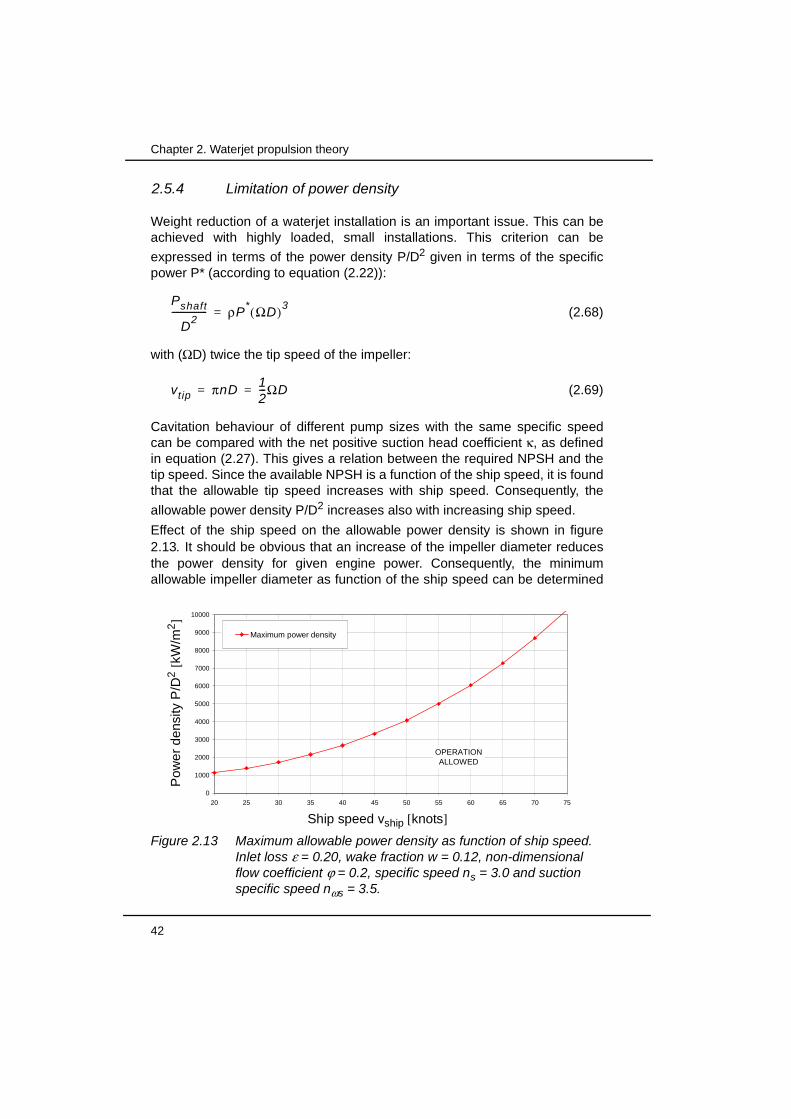
42
Chapter 2. Waterjet propulsion theory
2.5.4 Limitation of power density
Weight reduction of a waterjet installation is an important issue. This can beachieved with highly loaded, small installations. This criterion can be
expressed in terms of the power density P/D2 given in terms of the specificpower P* (according to equation (2.22)):
(2.68)
with (ΩD) twice the tip speed of the impeller:
(2.69)
Cavitation behaviour of different pump sizes with the same specific speedcan be compared with the net positive suction head coefficient κ, as definedin equation (2.27). This gives a relation between the required NPSH and thetip speed. Since the available NPSH is a function of the ship speed, it is foundthat the allowable tip speed increases with ship speed. Consequently, the
allowable power density P/D2 increases also with increasing ship speed.
Effect of the ship speed on the allowable power density is shown in figure2.13. It should be obvious that an increase of the impeller diameter reducesthe power density for given engine power. Consequently, the minimumallowable impeller diameter as function of the ship speed can be determined
Pshaft
D2
---------------- ρP* ΩD( )3
=
vtip πnD 12---ΩD= =
Figure 2.13 Maximum allowable power density as function of ship speed. Inlet loss ε = 0.20, wake fraction w = 0.12, non-dimensional flow coefficient ϕ = 0.2, specific speed ns = 3.0 and suction specific speed nωs = 3.5.
0
1000
2000
3000
4000
5000
6000
7000
8000
9000
10000
20 25 30 35 40 45 50 55 60 65 70 75
Maximum power density
OPERATIONALLOWED
Ship speed vship [knots]
Pow
er d
ensi
ty P
/D2
[kW
/m2 ]

2.6 Waterjet selection
Numerical analysis of a waterjet propulsion system 43
from the power density. It is found that the minimum allowable size dependson the cavitation behaviour of the pump, the ship speed and the powerapplied to the pump.
2.6 Waterjet selection
Up to this point, the entire analysis has been based on optimal performanceat one single design operating condition. In many cases waterjet installationshave multiple operating points. If the waterjets are applied for example inlarge fast ferries or planing hulls, the resistance line is quite different from theone of a regular displacement vessel. There is an additional resistance at aspeed range between about 20 and 30 knots. The speed, at which the localmaximum resistance occurs, is denoted as hump speed. The waterjetinstallation has to provide sufficient thrust to exceed the resistance at thehump speed. This requirement may lead to a larger waterjet than necessaryfor the design operating point.
In all shown examples, values for the wake fraction µ, pump efficiency ηpump,inlet losses, etc., have been considered as constants. In actual installationsall these parameters depend on the ship speed and/or the flow rate Q throughthe installation. Implementation of all of these dependencies will result in acomplex waterjet performance prediction program.
For a realistic comparison of various installations with different sizes over thecomplete range of ship speeds, such program should be used in order to takethe actual values for the loss coefficients and the efficiencies into account.
Figure 2.14 shows the output of a waterjet performance prediction programas used at the authors’ company for three different sized waterjets. The thrustis kept constant and the size is changed to show the effect of power densityon the cavitation margins. The hatched area represents the non-continuousoperational region. In this region severe cavitation in the waterjet will bepresent. The upper line represents the thrust breakdown line and the lowerline of this area is denoted as the 1% cavitation line. Thrust breakdownoccurs when the mass flow through the system collapses due to extremecavitation.
In the same figure an indication of a typical resistance curve of a fast ferry isplotted. The increased resistance at the hump speed of 25 knots can benoticed. The effect of waterjet size is obvious from this figure. The resistanceat the hump speed is about equal to the maximum thrust of the small waterjet.This means that the vessel has no extra thrust available to accelerate. Themaximum speed will not exceed 25 knots in this case, which is only 55% ofthe design speed. The larger waterjets, with lower power densities, havesufficient margin up to the design speed. To get a good balance betweencavitation performance and weight of the installation, the mid-size jet will beselected for this application.

44
Chapter 2. Waterjet propulsion theory
2.7 Closing remark
All equations and empirical values in this chapter are based on a uniforminflow to the pump. However, the inflow velocity field of a waterjet shows astrong non-uniform distribution, with variations in radial and tangentialdirection. This inflow might have an influence on the empirical values or thepump performance itself. Effects of the non-uniformity on pump performancewill be reviewed in more detail in chapter 7, where the complete waterjetinstallation is analysed numerically.
2.8 Nomenclature
A area m2
cf(l) local wall friction coefficient -
D diameter m
F force N
g gravitational acceleration m/s2
H pump head m
hj nozzle elevation m
IVR inlet velocity ratio (vship/vpump) -
l wetted length m
NPSH Nett positive suction head m
0%
20%
40%
60%
80%
100%
120%
140%
160%
180%
0 5 10 15 20 25 30 35 40 45 50
P/D^2 = 7000 kW/m^2
P/D^2 = 5000 kW/m^2
P/D^2 = 3000 kW/m^2
Resitance
P/D2 =7000
kW/m2
P/D2 =5000
Figure 2.14 Maximum thrust curves for three different waterjet sizes and resistance curves for fast ferry.
Ship speed vship [knots]
Thr
ust [
%]
7000 kW/m2
5000 kW/m2
3000 kW/m2

2.8 Nomenclature
Numerical analysis of a waterjet propulsion system 45
nω pump specific speed -
nωs suction specific speed -
n propeller/pump shaft speed 1/s
n boundary layer power law exponent -
P power W
P* specific power -
p pressure N/m2
Q volume flow rate m3/s
R resistance N
Rel Reynolds number based on length -
T thrust N
t thrust deduction factor -
U∞ undisturbed free stream velocity m/s
v velocity m/s
w momentum wake fraction -
z distance normal to the wall m
Greek symbols
δ specific pump diameter -
δ boundary layer thickness m
δ1 boundary layer displacement thickness m
δ2 boundary layer momentum thickness m
δ3 boundary layer energy thickness m
ε inlet loss coefficient -
φ momentum flux N
φ nozzle loss coefficient -
η efficiency -
ϕ flow coefficient -
κ net positive suction head coefficient -
µ jet velocity ratio -
ρ fluid density kg/m3
σ Thoma number -
τw wall shear stress N/m2
Ω angular velocity rad/s
ψ head coefficient -
Subscripts
1 inflow plane

46
Chapter 2. Waterjet propulsion theory
A available
in inflow
ind induced
out outlet / nozzle
prop propeller
R required
tube streamtube
wj,all complete waterjet structure
wj,hull excluded part of waterjet streamtube control volume
wj,tube included part of waterjet streamtube control volume
2.9 References
[1] Roberts, J.L. & Walker, G.J.,’Boundary layer ingestion in flush waterjetintakes’, Proceedings RINA Waterjet Propulsion II conference, Amster-dam, 1998
[2] Terwisga, T.J.C. van,’Waterjet hull interaction’, PhD thesis, Delft Uni-versity,1996
[3] Wilson, M.B., Chesnakas, C., Gowing, S., Becnel, A.J., Purnell, J.G.,Stricker, J.G., ‘Analysis of hull boundary layer velocity distributions withand without active waterjet inlets’, RINA Waterjet IV conference, Lon-don, 2004
[4] Schlichting, H., ‘Boundary layer theory’, McGraw-Hill, New York, 1968
[5] Fox, R.W., & McDonald, A.T.,’Introduction to fluid mechanics’, ThirdEdition, John Wiley & Sons, New York, 1985
[6] Newman, J.N., ‘Marine hydrodynamics’, MIT press, Cambridge, 1977
[7] Svensson, R. & Grossi, L.,’Trial result including wake measurementsfrom the world’s largest waterjet installation’, Proceedings RINA Water-jet Propulsion II conference, Amsterdam, 1998
[8] Seil, G.J., ‘Development of waterjet inlets for 100 knots’, ProceedingsFAST’99 conference, pp. 853-868, Seattle, 1999
[9] Bulten, N. & Verbeek, R.,’Design of optimal inlet duct geometry basedon operational profile’, Proceedings FAST2003 conference Vol I, ses-sion A2, pp 35-40, Ischia, Italy, 2003
[10] Verbeek, R.,’Application of waterjets in high-speed craft’, in Hydrody-namics: Computations, Model Tests and Reality, H.J.J. van den Boom(Editor) Elsevier Science Publication, 1992

2.9 References
Numerical analysis of a waterjet propulsion system 47
[11] Stepanoff, A.J., ‘Centrifugal and axial pumps; theory, design and appli-cation’, John Wiley & Sons, New York, 1957
[12] Wislicenus, G.F., ‘Fluid mechanics of turbomachinery’, Dover, NewYork, 1965
[13] MacPherson, D.M., ‘A universal parametric model for waterjet perform-ance’, Proceedings FAST’99 conference, pp. 879-882, Seattle, 1999
[14] Bohl, W.,’Strömungsmachinen (Aufbau und Wirkungsweise)’, Vogelverlag, Würzburg, 1977
[15] Arnold, J., Nijhuis, G.J., ‘Selection, design and operation of rotody-namic pumps’, Published by Nijhuis Pompen, first edition, 2005
[16] Gülich, J.F., ‘Kreiselpumpen’, Springer Verlag, Berlin, 1999
[17] Os, M.J. van,’On the flow and cavitation inception of mixed-flow impel-lers’, PhD thesis, Twente University, 1997
[18] Lewis, E.V., ‘Principles of naval architecture’, Volume II, Society ofNaval Architects and Marine Engineers, Jersey City, 1998
[19] Verbeek, R.,’Waterjet forces and transom flange design’, RINA water-jet propulsion conference, London, 1994

48
Chapter 2. Waterjet propulsion theory
Numerical analysis of a waterjet propulsion system 49
Chapter 3 Non-uniform distribution of pump entrance velocity field
The theory as presented in chapter 2 is based on experience with pumps withuniform inflow. It is known that in normal operating conditions the inflowvelocity in waterjet pumps is far from uniform. The first developers ofwaterjets have accepted this phenomenon; most probably since it has clearsimilarities with a ship-propeller wake field.
In the following subsection some methods will be presented to represent thenon-uniform pump inflow velocity distribution. With such representation it ispossible to derive an estimation of the flow rate fluctuations through animpeller channel and the variations of the inflow angle at the leading edge ofthe blade.
Obviously, the non-uniformity should be kept minimal from a hydrodynamicpoint of view. Therefore, a thorough analysis of the contributing factors to thenon-uniformity is made. In section 3.4 it will be shown that the majorcontributions are unavoidable in waterjet applications with flush type inlets.
3.1 Representation of non-uniform velocity distribution
In order to get an impression of the type of non-uniform velocity distributionsdiscussed here, typical distributions will be shown in this section. Thedistributions are derived from experimental results. The distributions can beexpressed as non-dimensional parameters or with a two-dimensionalrepresentation. Both methods will be discussed in this section as well.

50
Chapter 3. Non-uniform distribution of pump entrance velocity field
3.1.1 Experimental set-up
Measurements have been carried out on a model scale inlet, which ismounted on the Tom Fink cavitation tunnel [1]. A sketch of the test set-up isshown in figure 3.1. The model scale inlet has an inlet diameter of 150 mm. Inthe model scale test-rig the actual waterjet pump is not included. Though, theimpeller drive shaft, with a diameter of 22 mm, is included in the test set-up.The tunnel has a square cross-section of 600 x 600 mm.
At a cross-sectional plane just upstream of the pump, which will be denotedas impeller plane, the velocity distribution is measured with a 3 hole Pitot-tube.
Experiments have been carried out with a constant tunnel speed vtunnel of 8m/s. Upstream of the inlet an serrated edge is applied to thicken the naturaltunnel wall boundary layer. The shape of the edge is selected after anextensive test procedure. During the tests the growth of the boundary layerthickness and the smoothness of the profiles was evaluated.
The mass flow through the inlet is adjusted to get the desired IVR values, asdefined in equation (2.12). The tunnel vtunnel is used to represent the shipspeed vship. The measured conditions are listed in the table below. Reynoldsnumber for these conditions is based on the diameter of the inlet D and theaveraged pump velocity vpump.
Figure 3.2 shows the axial velocity distributions for two inlet velocity ratios,derived from the measurements. The condition with an IVR of 1.68represents a normal cruising speed of a fast ferry. The figure on the rightshows the distribution at very high IVR. This condition can occur in highspeed motor yacht applications (> 60 knots). It should be noted that the shaft
Figure 3.1 Sketch of test setup with inlet mounted on top of cavitation tunnel
pitot-tube
vtunnel
vpump
Z
x y
z
pref

3.1 Representation of non-uniform velocity distribution
Numerical analysis of a waterjet propulsion system 51
diameter (d=22 mm) is about half the diameter of the non measured (blank)region. Moreover, it should be taken into account that the shaft was notrotating during experiments, which results in a symmetric velocity profile.
Similar velocity distributions are found for another inlet geometry in this test-rig. The measurements in the cavitation tunnel indicate that the level of non-uniformity is almost independent of the actual inlet geometry. Measurementsin a windtunnel with systematic changes of the geometry confirm thisbehaviour [2]. It is concluded that the non-uniformity is strongly related to theinlet velocity ratio and only weakly related to the precise shape of the inlet.
Based on a survey of the available (confidential) experimental and numericaldata at the authors’ company, it is concluded that within the design space forcommercial applications all possible inlet geometries show more or less thesame type of velocity distribution.
Table 3.1 Parameters of conditions of the measured velocitydistributions
IVR[-]
Vtunnel[m/s]
Vpump[m/s]
Reinl [-]
1.68 8.00 4.76 7.14 x 10⁵
1.87 8.00 4.28 6.42 x 10⁵
2.03 8.00 3.94 5.91 x 10⁵
2.19 8.00 3.65 5.48 x 10⁵
Figure 3.2 Experimentally determined non-uniform velocity distributions for 2 IVR conditions. Left: medium IVR of 1.68, right high IVR of 2.19.
y
z

52
Chapter 3. Non-uniform distribution of pump entrance velocity field
3.1.2 Non-dimensional representation
For easy comparison of different inlet geometries and operating conditions,the level of non-uniformity is expressed as a single value ζ [3]:
(3.1)
where v is the local axial velocity and vpump the average axial velocity. Therelation between non-uniformity and IVR can be assessed with thisparameter.
3.1.3 Two-dimensional representation
Hu&Zangeneh [4] use a circumferentially averaged velocity distribution toinvestigate the effects of the non-uniform velocity distribution on the waterjetpump performance. However, for a detailed analysis of the time-dependenteffects of non-uniformity on pump performance, this quantification is notsufficient. At least a two dimensional description, based on the radius r andthe angle θ, of the inflow field in front of the impeller is required to capture thetime varying phenomena.
Such a description of the axial velocity distribution can be obtained if thevelocity field is approximated as a Fourier series:
(3.2)
where the coefficients an(r) are taken as quadratic functions of the radius andm is the number of harmonics. For the present Fourier approximation 4harmonics have been used. The quadratic functions an(r) are based oncoefficients at five different radii. Results of the two dimensional velocity fielddescription are shown in figure 3.3 for the condition IVR=2.19 together withthe measured values.
Agreement between measurements and the numerical approximation issatisfactory for all radii along the complete circumference. A similaragreement is found at lower IVR.
ζ 1Q---- v vpump–( )2
Ad∫≡
vx r θ,( ) a0 r( ) an r( ) nθ( )cos( )
n 1=
m
∑+=

3.2 Local flow rate fluctuations
Numerical analysis of a waterjet propulsion system 53
3.2 Local flow rate fluctuations
It is expected that the non-uniform inflow velocity distribution will result in avarying flow rate through the channels between the impeller blades during arevolution. The amplitude of the fluctuation is not only dependent on the levelof non-uniformity of the velocity distribution but also on the number of impellerblades. An estimation of the channel flow rate as function of the rotor positioncan be calculated with:
(3.3)
where the axial velocity vx is integrated over the impeller passage inlet area,with N the number of impeller blades, Qbb the volume flow rate in an impellerchannel, r1 the hub radius and r2 the tip radius at the impeller inlet.
Figure 3.3 Comparison of axial velocity derived from measurements with the velocities based on Fourier series for velocity distribution at IVR = 2.19
0
0.2
0.4
0.6
0.8
1
1.2
1.4
1.6
0 45 90 135 180 225 270 315 360
Measurement r=20 mm Fourier r=20 mmMeasurement r=40 mm Fourier r=40 mmMeasurement r=55 mm Fourier r=55 mmMeasurement r=65 mm Fourier r=65 mmMeasurement r=70 mm Fourier r=70 mm
Angle θ [degrees]
v x(r
,θ)/
v pum
p [-
]
Qbb vx r θ,( ) r⋅ r θdd
r1
r2
∫θ π
N----–
θ πN----+
∫=
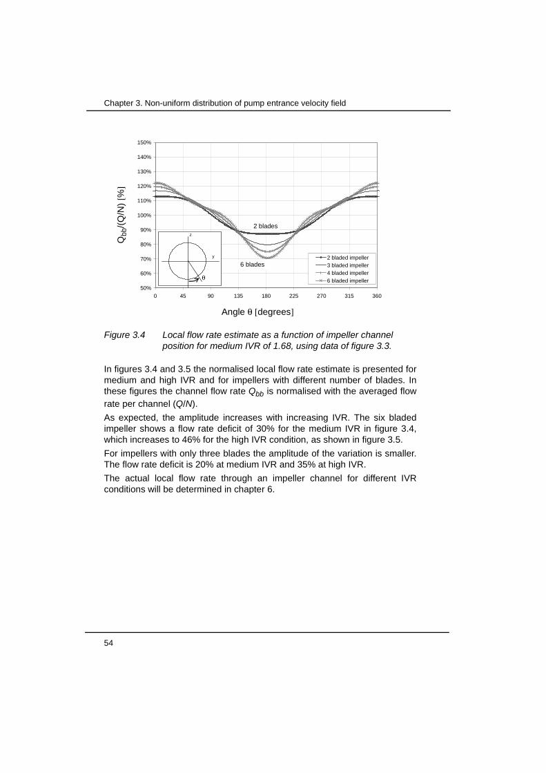
54
Chapter 3. Non-uniform distribution of pump entrance velocity field
In figures 3.4 and 3.5 the normalised local flow rate estimate is presented formedium and high IVR and for impellers with different number of blades. Inthese figures the channel flow rate Qbb is normalised with the averaged flowrate per channel (Q/N).
As expected, the amplitude increases with increasing IVR. The six bladedimpeller shows a flow rate deficit of 30% for the medium IVR in figure 3.4,which increases to 46% for the high IVR condition, as shown in figure 3.5.
For impellers with only three blades the amplitude of the variation is smaller.The flow rate deficit is 20% at medium IVR and 35% at high IVR.
The actual local flow rate through an impeller channel for different IVRconditions will be determined in chapter 6.
50%
60%
70%
80%
90%
100%
110%
120%
130%
140%
150%
0 45 90 135 180 225 270 315 360
2 bladed impeller3 bladed impeller4 bladed impeller6 bladed impeller
y
z
Figure 3.4 Local flow rate estimate as a function of impeller channel position for medium IVR of 1.68, using data of figure 3.3.
Angle θ [degrees]
Qbb
/(Q
/N)
[%]
θ
2 blades
6 blades

3.3 Impeller velocity triangles
Numerical analysis of a waterjet propulsion system 55
3.3 Impeller velocity triangles
The axial velocity distribution can be used to derive the fluctuations in inletflow angles. This angle determines for a great deal the loading of the impellerblade. A lower inlet flow angle will lead to higher blade loading in general.Moreover the cavitation behaviour of the impeller will depend on thefluctuations of the inflow angle.
The design inlet blade angle is based on the inlet velocity triangle withuniform flow and without pre-rotation, as shown in figure 3.6:
(3.4)
50%
60%
70%
80%
90%
100%
110%
120%
130%
140%
150%
0 45 90 135 180 225 270 315 360
2 bladed impeller
3 bladed impeller
4 bladed impeller
6 bladed impeller
y
z
Figure 3.5 Local flow rate estimate as a function of impeller channel position for high IVR of 2.19, using data of figure 3.3.
Angle θ [degrees]
Qbb
/(Q
/N)
[%]
θ
2 blades
6 blades
Figure 3.6 Velocity triangle of inlet flow angle.
vx
Ωr
βdesign
βdesign
vx
Ωr------ atan=
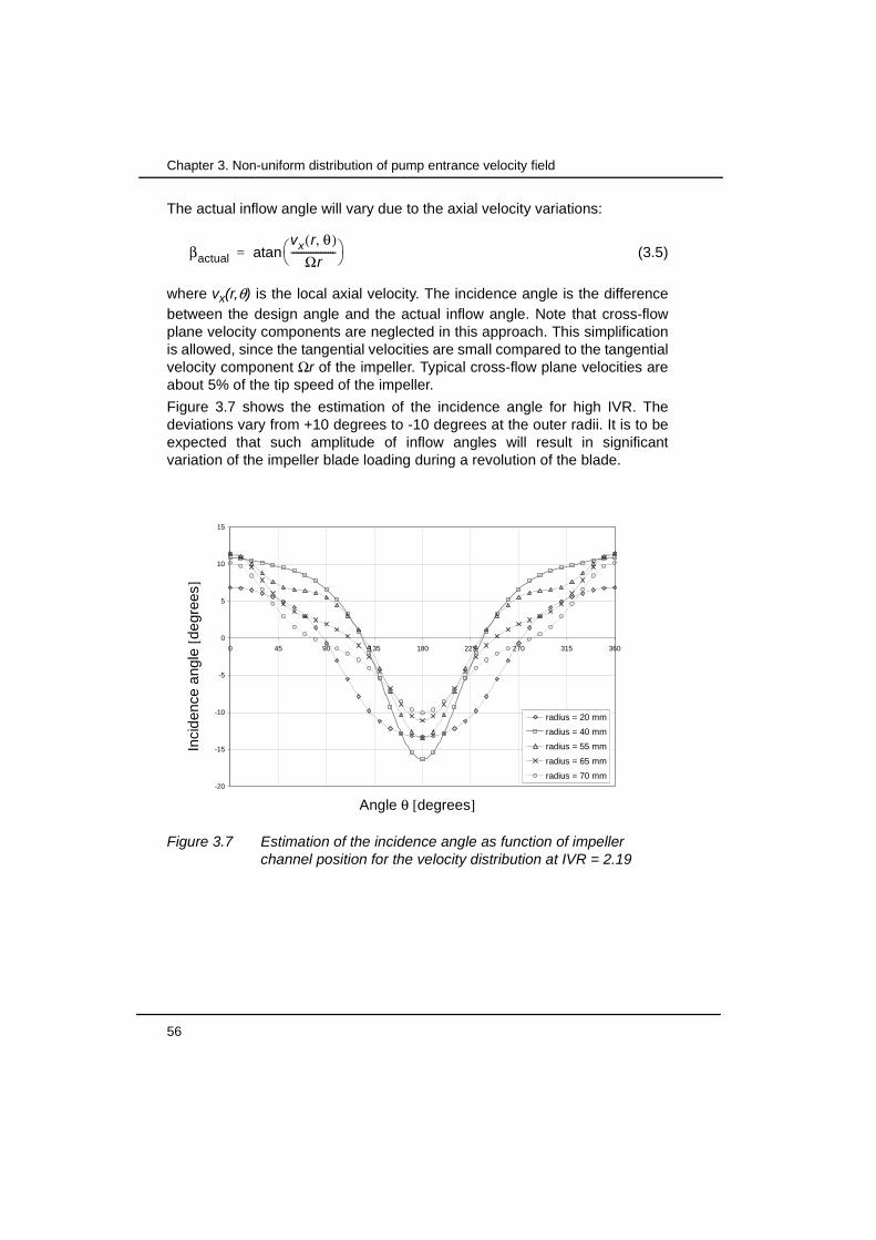
56
Chapter 3. Non-uniform distribution of pump entrance velocity field
The actual inflow angle will vary due to the axial velocity variations:
(3.5)
where vx(r,θ) is the local axial velocity. The incidence angle is the differencebetween the design angle and the actual inflow angle. Note that cross-flowplane velocity components are neglected in this approach. This simplificationis allowed, since the tangential velocities are small compared to the tangentialvelocity component Ωr of the impeller. Typical cross-flow plane velocities areabout 5% of the tip speed of the impeller.
Figure 3.7 shows the estimation of the incidence angle for high IVR. Thedeviations vary from +10 degrees to -10 degrees at the outer radii. It is to beexpected that such amplitude of inflow angles will result in significantvariation of the impeller blade loading during a revolution of the blade.
βactual
vx r θ,( )Ωr
------------------ atan=
Figure 3.7 Estimation of the incidence angle as function of impeller channel position for the velocity distribution at IVR = 2.19
-20
-15
-10
-5
0
5
10
15
0 45 90 135 180 225 270 315 360
radius = 20 mm
radius = 40 mm
radius = 55 mm
radius = 65 mm
radius = 70 mm
Angle θ [degrees]
Inci
denc
e an
gle
[deg
rees
]

3.4 Origin of the non-uniform velocity distribution
Numerical analysis of a waterjet propulsion system 57
3.4 Origin of the non-uniform velocity distribution
The development of the non-uniform velocity distribution can be explainedwith basic fluid dynamics theory. There are four phenomena which contributeto the non-uniformity of the velocity distribution:
1. boundary layer ingestion2. deceleration of the flow 3. obstruction of the flow due to the shaft4. bend in the inlet duct
A sketch of the phenomena is presented in figure 3.8. The above items arediscussed in more detail in the remainder of this section.
3.4.1 Boundary layer ingestion
Waterjets with flush mounted inlet ducts ingest water from the boundary layerbelow the hull. A typical ship speed for a waterjet propelled vessel is 40 knots(about 20 m/s). With a wetted length of 80 m, the Reynolds number becomes
1.6 x 10⁹. At these high Reynolds numbers the boundary layer thickness canbe approximated with a power law velocity distribution, as shown in equation(2.3), with a power n of about 10.
The contribution of the boundary layer ingestion to the non-uniformitydepends on the amount of water that is ingested from the boundary layer.The ingestion of boundary layer water can be expressed with the ratiobetween the suction depth h and the boundary layer thickness δ. If this ratio(h/δ) is smaller than 1, then all the water is taken from the hull boundary layer.
4
2
1
3
Figure 3.8 Phenomena which contribute to development of a non-uniform inflow velocity distribution to the pump. 1. boundary layer ingestion. 2. deceleration of the flow. 3. obstruction of the flow by shaft. 4. bend in duct.
h
58
Chapter 3. Non-uniform distribution of pump entrance velocity field
The suction depth h depends on the total ingested volume flow rate and theassumed shape of the streamtube. As mentioned before, waterjetmanufacturers and ship model basins use a simplified method, in which theshape of the streamtube is approximated as a rectangular box with a width of1.3 times the inlet diameter.
When the suction depth h is smaller than the boundary layer thickness, thesuction depth h is calculated with:
(3.6)
where Q is the volume flow, vship the undisturbed velocity and λD theassumed width of the rectangular box with λ equal to 1.3.
If the suction depth h exceeds the boundary layer thickness, then thedisplacement thickness can be used to calculate the suction depth h:
(3.7)
The relations for the boundary layer thickness (for example equation (2.10)for n=9) show that the length of the vessel has a major influence on thedevelopment of the boundary layer. This effect is shown more clearly in figure3.9, where the boundary layer ingestion ratio h/δ is shown for three differentvessel lengths. The flow rate Q is adjusted for each ship speed, to take theeffect of increasing flow rate with increasing ship speed into account.
The ratio h/δ decreases with ship speed for all ship lengths. With higherincoming velocity and constant suction box width, the suction height h willreduce.
It can be seen that the boundary layer ingestion ratio h/δ is about 0.90 at 45knots for the short vessel. The ratio is reduced to 0.50 when the length isdoubled. Since the velocity profile has the largest gradients near the wall, thisresults in increased non-uniformity, for longer vessels. Decrease of theboundary layer ingestion ratio h/δ is coupled to an increase of IVR. As aconsequence, the non-uniformity will increase with increasing IVR as well.
3.4.2 Deceleration of the flow
Waterjets operate in IVR conditions of 1.3 to 1.8 in general. The averagedvelocity of the water just in front of the pump is thus smaller than the shipspeed. Even if the velocity in front of the pump is compared with the massaveraged incoming velocity, which is smaller due to boundary layerdevelopment, there is still a significant retardation of the flow in the inlet duct.The retardation of the flow can be regarded as a (subsonic) diffuser flow
hQ
vshipλD-------------------- n 1+
n------------ δ1 n⁄⋅ ⋅
n n 1+( )⁄ h δ<( )=
h QvshipλD-------------------- δ1+
QvshipλD-------------------- δ
n 1+------------ h δ>( )+= =

3.4 Origin of the non-uniform velocity distribution
Numerical analysis of a waterjet propulsion system 59
phenomenon. According to the theory of standard diffusors, the velocityprofile in a conventional diffusor depends on the diffusor angle. Nikuradsemeasured the velocity profiles in convergent and divergent channels withdiffusor angles between -4° and +8° (shown in Schlichting [5]). The velocityprofiles in convergent channels, which have negative diffusor angles, becomemore uniform. In contrast, the velocity profile becomes less uniform indivergent channels (or in other words, it corresponds to a lower n value in apower law profile). Therefore, retardation of the flow increases the level ofnon-uniformity in the velocity distribution. Consequently, the increase of non-uniformity is related to the value of IVR.
The standard diffusor theory assumes a uniform inflow at the entrance of thediffusor. However in a waterjet the boundary layer creates a non-uniformdistribution at the beginning of the diffusor. When a velocity profile is non-uniform at the entrance a diffusor, the level of non-uniformity will evenincrease. This phenomenon is explained by Betz [6] with a simple example.
3.4.3 Obstruction of the flow due to the shaft
The impeller shaft forms an obstruction of the flow in the inlet, comparable toa propeller shaft in a ship. A narrow wake region with low velocity is foundnear the shaft. If the pump shaft is equipped with a stationary sleeve, then itcan lead to unstable vortex shedding. Hu & Zangeneh [7] and Seil [8]
0.00
0.25
0.50
0.75
1.00
1.25
1.50
25 30 35 40 45 50
0.5
0.75
1
1.25
1.5
1.75
2
Wetted length 50 mWetted length 75 mWetted length 100 mIVR
Figure 3.9 Boundary layer ingestion ratio h/δ for three different vessel lengths l as function of ship speed vship with corresponding IVR.
Ship speed [knots]
IVR
[-]
h/δ
[-]

60
Chapter 3. Non-uniform distribution of pump entrance velocity field
investigated the effect of the rotation of the shaft. They show that the flowstabilizes due to rotation of the shaft. In general a waterjet installation doesnot have a stationary sleeve around the shaft, so a stable flow is found in thevicinity of the shaft.
3.4.4 Bend in the inlet duct
The fourth contributing factor to the non-uniform velocity distribution is thebend in the inlet duct. Inside the bend a variation in velocity is found betweenthe inner and outer part of the bend. This non-uniformity will restore to acertain extent downstream of the bend. In a waterjet however, the length ofthe cylindrical pipe between the bend and the pump is in general smaller thanthe inlet diameter. As a result part of the created non-uniformity due to thebend remains in the velocity distribution.
The convex shape of the first part of the roof of the inlet may be regarded asa bend as well, which might have a positive influence on the velocitydistribution. The radius of curvature is about six times larger than the radiusof curvature of the bend, so the effect of this curvature can be neglected inthe analysis and is therefore not marked in figure 3.8.
3.4.5 Closing remark
The major contributions to the non-uniformity are caused by the IVR relatedphenomena of boundary layer ingestion and retardation of the flow. As longas waterjets are operated at IVR values above 1.5, a substantial non-uniformflow will exist.
3.5 Non-uniform inflow velocity distributions in otherturbo machinery
In the literature relatively little attention has been paid so far to the effects ofnon-uniform inflow to the waterjet pump. This may be attributed to its closerelation to the conventional ship propeller, which also operates in a non-uniform wake field in general. This wake field is determined by the shape ofthe vessel, so the propulsion system designer has to cope with it. A lot ofresearch has been done on the effects of non-uniform inflow to a shippropeller already. For example the work of Van Manen [9] in the 1950s can bementioned. Variations in effective inflow angle for the tested propeller werebetween -1° and +4°. This range is significantly smaller than the expectedvariations for the waterjet pump, as shown in figure 3.7.
Non-uniform inflow to mixed-flow or centrifugal pumps may occur if the pumpis mounted close to an upstream disturbance, like a pipe bend. For anacceptable inflow to the pump, most manufacturers prescribe a minimum

3.6 Nomenclature
Numerical analysis of a waterjet propulsion system 61
required length of straight pipe on the suction side of the pump, typicallyseveral pipe diameters long. Examples can be found in a pump handbook ofSulzer [10]. The use of an acceleration nozzle just upstream of the pump isalso recommended to enhance the uniformity of the inflow for certain types ofpumps.
The requirement of long straight suction pipes can not always be met, like theflow into the first stage of a boiler feed pump. Cooper [11] shows thecalculated flow pattern at the exit of a radial inlet passageway for such apump. A maximum velocity of 1.75 times the average inflow velocity is foundfor this example. This level of non-uniformity seems to be more in line withthat found in waterjet applications. Similar flow phenomena will occur indouble suction pumps and inline pumps.
Another typical inflow is found for pumps with a sump, as used in coolingwater pump applications in power stations. Here a suitable design of theinflow and inlet chamber is to obtain an acceptable inflow pattern. Additionalacceleration can be applied for further improvement.
3.6 Nomenclature
A area m2
D diameter m
h suction depth m
IVR inlet velocity ratio (vship/vpump) -
N number of impeller blades -
n boundary layer power law value -
Q flow rate m3/s
Qbb channel flow rate -
r radius m
v velocity m/s
Greek symbols
β blade angle rad
δ boundary layer thickness m
δ1 boundary layer displacement thickness m
θ angle rad
λ suction tube width factor -
ζ non-uniformity -
Ω angular velocity rad/s
62
Chapter 3. Non-uniform distribution of pump entrance velocity field
Subscripts
x axial direction
3.7 References
[1] Brandner, P. & Walker, G.J., ‘A waterjet test loop for the Tom Fink cavi-tation tunnel’, Proceedings Waterjet Propulsion III conference, Gothen-burg, 2001
[2] Bulten, N.W.H.,‘Influence of boundary layer ingestion on waterjet per-formance parameters at high ship speeds’, Proceedings of the 5thinternational conference on Fast Sea Transportation, pp 883-892,Seattle, 1999
[3] Verbeek, R. & Bulten, N.W.H.,’Recent developments in waterjetdesign’, Proceedings RINA Waterjet Propulsion II conference, Amster-dam, 1998
[4] Hu, P. & Zangeneh, M.,’CFD calculation of the flow through a water-jetpump’, Proceedings Waterjet Propulsion III conference, Gothenburg,2001
[5] Schlichting, H.,’Boundary layer theory’, Mc Graw-Hill, New York, 1968
[6] Betz, A, ‘Introduction to the theory of flow machines’, Pergamon Press,Oxford, 1966
[7] Hu, P., Zangeneh, M., ‘Investigations of 3D turbulent flow inside andaround a water-jet intake duct under different operating conditions’,ASME Journal of Fluids Engineering, Vol 121, pp. 396-404, 1999
[8] Seil, G.J.,’The effect of the shaft, shaft rotation and scale on the flow inwaterjet inlets’, Proceedings Waterjet Propulsion III conference,Gothenburg, 2001
[9] Manen, J.D. van, ’Invloed van de ongelijkmatigheid van het snelheids-veld op het ontwerp van scheepsschroeven’, PhD thesis, Wageningen,1951
[10] Sulzer Brothers Ltd, ‘Sulzer centrifugal pump handbook’, ElsevierApplied Science, London, 1989
[11] Cooper, P.,’Perspective: the new face of R&D - A case study of thepump industry’, ASME Journal of Fluids Engineering, Vol 118, pp. 654-664, 1996

Numerical analysis of a waterjet propulsion system 63
Chapter 4 Mathematical treatment
To get more insight in the behaviour of the flow through a waterjet installation,experiments can be done and calculations can be made. With anexperimental set-up of a waterjet inlet velocity, pressure and forces can bemeasured. In this thesis, however these quantities will be determined bynumerical simulations.
A numerical method is based on a mathematical model of the physics of theflow. It constitutes a set of governing equations derived from first principles,often complemented with empirical relations. The numerical method isobtained by discretisation of the governing equations. The present type offlow can be described by the Navier-Stokes equations. Before these equationcan be solved numerically for the application of interest, it is necessary tomake some simplifications. A review of the important flow features is given insection 4.1 to get an impression of the feasible simplifications without majorloss of accuracy. This analysis will result in a selection of the best suitablemathematical method. The chosen method will be described in more detail insection 4.3. Some known weaknesses of the mathematical method will bediscussed in more detail to get an indication of the obtainable accuracy.
4.1 Requirements of mathematical method
In this section the requirements for the mathematical method will beformulated. The goal of the mathematical analysis is the prediction of the flowthrough a waterjet installation. Based on the different requirements for theprediction three different mathematical methods will be evaluated: the

64
Chapter 4. Mathematical treatment
potential flow model, the model based on the Euler flow and the model basedon the Reynolds averaged Navier-Stokes (RANS) equations. RANS methodsare also denoted as viscous methods, whereas the other two methods do notinclude terms due to viscosity and heat conduction. They require, for exampleeffects of viscosity, such as flow separation, to be modelled. In potential flowmethods, the flow is irrotational, i.e. the vorticity equals zero everywhere,except in infinitesimal regions such as vortex sheets and vortex filaments.
4.1.1 Incompressibility
The first requirement for the mathematical method is the capability ofhandling incompressible flow. The maximum velocity in a full scale waterjetinstallation is about 50 m/s, which is much smaller than the speed of sound inwater, which is about 1450 m/s. The resulting Mach number is thussufficiently small to treat the flow as incompressible. It is noted that the speedof sound is based on a non-cavitating flow. In a cavitating flow, the speed ofsound reduces significantly, which results in a compressible flow behaviour.
All three mentioned mathematical methods can satisfy this requirement.Nevertheless it can be mentioned that this requirement represents one of themajor differences between pumps and compressors, as discussed in section1.2. mathematical methods for compressor analysis cannot be used directlyfor incompressible flow. For compressible flow the Euler equations arehyperbolic in time for any Mach number. This gives the opportunity to use asingle numerical technique for subsonic, supersonic or mixed subsonic-supersonic (transonic) flow problems [1]. These methods are commonlycalled time marching methods. In these methods compressibility is employed,which results in amongst others travelling pressure waves through thedomain. In an incompressible flow, pressure fluctuations are instantaneous inthe whole domain. Reconditioning, i.e. some form of artificial compressibilityhas to be introduced in the compressible flow solver in order to analyse anincompressible flow.
4.1.2 High Reynolds number
For full scale waterjet installations the typical Reynolds numbers for the inletand the impeller are both very large. For the impeller the Reynolds number isdefined as:
(4.1)
where ρ is the density, µ the dynamic viscosity, vtip is the tip speed of theimpeller blade and Dinl the diameter of the inlet at the pump suction side. For
Reimp
ρvtipDinl
µ----------------------=

4.1 Requirements of mathematical method
Numerical analysis of a waterjet propulsion system 65
typical waterjet applications the tip speed can be about 50 m/s. For an inlet
diameter of 1.2 m this gives a Reynolds number Reimp of 6x10⁷.
Calculation of the Reynolds number that characterises the flow in the inletrequires another typical velocity. This can be either the ship speed or thepump speed (as defined in equation (2.11)). The actual choice is not socritical, since both values do not differ by more than a factor of two. In order torepresent the flow phenomena inside the inlet best, the Reynolds number forthe inlet is defined as:
(4.2)
For the same typical configuration as above, the Reynolds number Reinl will
be about 107, which is 6 times smaller than the impeller Reynolds number.Model scale experiments are performed at lower Reynolds numbers, as
shown in table 3.1 on page 51. These values still exceed 5x10⁵, which can beregarded as high Reynolds number flow. It is to be expected that, at least atdesign conditions, viscous effects play a limited role.
4.1.3 Time dependency
There are two different reasons for the flow to be time-dependent in awaterjet installation: (i) the non-uniformity of the flow at the impeller entranceresults in a time varying onset flow of the rotating blades and (ii) theinteraction between moving rotor and stationary stator blades at the impelleroutlet is unsteady. In the rotating frame of reference, phenomena associatedwith the first reason have a frequency related to the shaft frequency. Thefrequency of the interaction phenomena between the rotor and stator bladesdepends on the number of stator blades and the shaft frequency.
In the stationary frame of reference the frequency of the fluctuations due torotor-stator interaction is related to the number of impeller blades. The effectof the non-uniform inflow will give a steady component with superposedfluctuations with the blade passing frequencies.
4.1.4 Non-uniformity of impeller inflow
In chapter 3 the velocity distribution upstream of the impeller is discussed. Itis shown that the velocity field is strongly non-uniform even at normal waterjetoperating conditions. This velocity distribution has to be reproduced by themathematical method in order to obtain a correct prediction of the inlet flowphenomena. For an analysis of the isolated pump, the non-uniform inflow tothe impeller has to be implemented as an inflow boundary condition.
Reinl
ρvpumpDinl
µ----------------------------=
66
Chapter 4. Mathematical treatment
The development of the velocity distribution in the inlet is attributed to theingestion of the boundary layer and to the deceleration of the flow.Generation of vorticity plays an important role in these flow phenomena.Application of a mathematical method based on the potential flow assumptionor an inviscid flow model is therefore not suitable for the analysis of inlet flowphenomena.
Potential flow analyses of mixed-flow pumps have been made by Van Esch[2] and Van Os [3]. These calculations are based on a uniform inflow velocitydistribution. Implementation of a non-uniform velocity distribution introducesvelocity gradients for the axial velocity component. The constraint ofirrotational flow results in additional velocity gradients in the directionsperpendicular to the axial inflow direction. The cross components of the inflowvelocity distribution have such a dominating influence on the overalldevelopment of the non-uniformity, that the velocity distribution is almostuniform within about one diameter pipe length. The analysis of the stability ofthe non-uniform velocity distribution is discussed in more detail in appendix A.
It is concluded that for the analysis of both a waterjet inlet as well as a pumpwith non-uniform inflow a suitable mathematical method should take thepresence of vorticity into account.
4.1.5 Tip clearance flow
In general, waterjets are equipped with unshrouded mixed-flow or axialimpellers. Unshrouded impellers have a small clearance between the bladetips and the stationary housing. This housing is called the seatring. Thepressure difference between the pressure and suction side of the bladecauses some leakage flow through the clearance. This leakage flow shouldbe kept as low as possible to maintain a high efficiency of the pump. Thedistance between the impeller tip and the seatring is therefore very small,about 1-2% of the diameter. On the other hand, the velocity differencebetween the rotating blade tip and the stationary seatring can be about 50 m/s, which leads to large velocity gradients in the clearance.
As a result of the available pressure difference between pressure and suctionside of the blade and the occurring viscous losses in the clearance a certainflow will establish. Effects of viscosity can not be neglected, if this flow is to bedetermined. Second effect of the viscosity is the development of boundarylayers on the blade tip and the seatring. This is confirmed by Kunz et al. [4] inthe investigation of tip clearance phenomena in an axial compressor cascadewith an Euler and a Navier-Stokes method. It is found that the Navier-Stokesmethod shows better agreement with experimental data than the Eulermethod. Prediction of the tip clearance mass flow rate is presumed to bemore accurate with the Navier-Stokes method.

4.2 Conservation laws
Numerical analysis of a waterjet propulsion system 67
The flow in a mixed-flow pump with various tip clearances has been analysedby Goto [5]. For this analysis he uses the unsteady Reynolds-averagedNavier-Stokes equations in a rotational frame of reference. Results of thecalculations show reasonably good agreement with the experimental data.Moreover a variety of jet-wake flow patterns at the exit of the impeller arepredicted well.
4.1.6 Final remarks
Based on the listed requirements and the capabilities of the different models,the choice for a viscous flow model is justified. In the next two chapters,results of a detailed validation study of numerical simulations for the waterjetinlet and the mixed-flow pump are presented. It is acknowledged that aviscous (i.e. RANS) flow method requires significantly more computationalresources than an Euler method and certainly much more than a potentialflow method.
Cavitation will not be taken into account in the analyses. Since cavitationmodels are presently developed for most commercial RANS codes, is it to beexpected that application of methods with some form of cavitation model willbe feasible in the near future.
The calculations presented in this study are carried out with the commercialCFD method Star-CD. This method is based on a finite volume numericalmethod. Both tetrahedral and hexahedral cell types can be used for themesh. In this study all meshes are generated with hexahedral cells only.
4.2 Conservation laws
To describe the flow phenomena in a waterjet installation, two conservationlaws are used. These are the laws for conservation of mass and that ofmomentum. Conservation of mass is also denoted as the continuity equation(see for example [6]):
(4.3)
where ρ is the density of the fluid and the velocity.
In many cases the flow can be assumed to be incompressible. This isallowed, whenever variations in density are small. These variations in densityare caused by variations in the pressure. Since in the present applications thevelocities are much smaller than the speed of sound in the water, which isabout 1450 m/s, the variation in density will be negligible. For anincompressible flow the continuity equation (4.3) reduces to:
(4.4)
t∂∂ρ ∇+ ρv⋅ 0=
v
∇ v⋅ 0=

68
Chapter 4. Mathematical treatment
Conservation of momentum is given by (see also [6]):
(4.5)
where p is the pressure, µ is the dynamic viscosity, which is assumed to beconstant in the derivation of equation (4.5) and is the acceleration of
gravity. This set of equations is known as the Navier-Stokes equation. For anincompressible flow, equation (4.4) can be substituted into equation (4.5).This results in the Navier-Stokes equation for incompressible flow:
(4.6)
The Navier-Stokes equation can be solved numerically directly without furtherassumptions. This requires direct numerical simulations (DNS) to obtain thetime-accurate solution of equations (4.4) and (4.6) on a grid that is sufficientlyfine to resolve all flow details. Such a method is not suitable for practicalengineering analyses, however. In the following section an approach will bediscussed, which enables numerical solution of the flow field, within apractical context.
4.3 Reynolds Averaged Navier-Stokes (RANS) flow
In order to convert the Navier-Stokes equations into a set of equations, thatcan be solved numerically for general engineering applications, the conceptof splitting the flow variables in a mean and a fluctuating part is employed.Substitution of this decomposition in the Navier-Stokes equation and timeaveraging the continuity and the Navier-Stokes equations, results in a set ofequations for the mean-flow field variables. The concept of time averagingwas introduced by Reynolds in 1895. The resulting equation is thereforecalled the Reynolds-averaged Navier-Stokes (RANS) equation.
4.3.1 Reynolds averaging
The principle of Reynolds averaging is based on a decomposition of thevariables in a time averaged value and a fluctuating part:
(4.7)
ρt∂
∂ v ρ v ∇⋅( )v+ ∇p– µ∇2v
13---µ∇ ∇ v⋅( ) ρg+ + +=
g
ρt∂
∂ v ρ v ∇⋅( )v+ p µ v ρg+∇2+∇–=
vi vi vi'+=

4.3 Reynolds Averaged Navier-Stokes (RANS) flow
Numerical analysis of a waterjet propulsion system 69
The time averaged variable is defined as:
(4.8)
where t1 has to be larger than the time scale of the smallest fluctuations.Therefore,
(4.9)
The average of the fluctuating part is zero by definition. Nevertheless, if theproduct of two variables is considered, not all fluctuating terms vanish whenthey are correlated, thus:
(4.10)
Substitution of the decomposed terms in the Navier-Stokes equation for thevelocity and pressure and application of the method of Reynolds averaginggives:
(4.11)
The term is called the Reynolds stress term, where is a diadic
product defined by . This tensor contains the correlations of the
fluctuating terms of the velocity components. The term with the Reynoldsstress can be treated in several ways. Boussinesq proposed a closurehypothesis for the Reynolds stress term. In index notation the closure isdefined as:
(4.12)
which is referred to as an eddy viscosity model with µT the turbulent or eddyviscosity and k the turbulent kinetic energy defined as:
(4.13)
Turbulence models are used to obtain a value for the eddy viscosity. Analternative approach is to derive from the original time-dependent Navier-
vi1T---
T t1→lim vi td
t
t T+
∫=
vi'1T--- vi vi–[ ]
t
t T+
∫T t1→lim dt 0= =
vivj vivj vi'vj'+=
ρt∂
∂ v ρ v ∇⋅( )+ v p µ v ρg ∇ ρ v'v'( )⋅–+∇2+∇–=
ρ v'v'( ) v'v'( )
v'v'( )i j vi'vj'=
ρvi'vj'– µT xj∂∂vi
xi∂∂vj+
2
3---ρkδi j–=
k 12--- vi'vi'( ) 1
2--- vx'vx' vy'vy' vz'vz'+ +( )= =

70
Chapter 4. Mathematical treatment
Stokes equations a transport equation for each of the Reynolds stresscomponents, however. These equations require another group of closurerelations before the equations can be solved numerically. Such a model iscalled a Reynolds stress turbulence model.
Substitution of equation (4.12) into the Reynolds averaged Navier-Stokesequation (4.11) gives:
(4.14)
The next step is the combination of the pressure term, the turbulent kineticenergy term and the gravitational term. The modified pressure is defined as:
(4.15)
where it is assumed that gravity is directed in the z-direction. The resultingNavier-Stokes equation with the Reynolds stress terms included, becomes:
(4.16)
where the molecular viscosity µ and turbulent viscosity µT have beencombined into the effective viscosity µeff.
4.3.2 Eddy viscosity turbulence models
Eddy viscosity turbulence models are used to determine a value for the eddyviscosity µT. Once this eddy viscosity is known, the Reynolds stresses areknown and consequently the Reynolds-averaged Navier-Stokes equationscan be solved. The available eddy viscosity turbulence models can be dividedinto 3 groups:
1. mixing length or algebraic models or zero-equation models2. one-equation models3. two-equation models
In a zero-equation model, the eddy viscosity µT is based on the mixing lengthconcept. This mixing length is based on algebraic relations. The eddyviscosity for an algebraic model is defined as:
(4.17)
where lmix is Prandtl’s mixing length.
ρt∂
∂ v ρ v ∇⋅( )v+ p ∇ µ µT+( ) v v∇( )T+∇( ) ρg ∇2
3---ρk–+⋅+∇–=
p∗ p23---ρk ρgz–+=
ρt∂
∂ v ρ v ∇⋅( )v+ p∗ ∇ µ⋅ eff ∇v ∇v( )T+( )+∇–=
µT ρlmix2 dv
dy------=

4.3 Reynolds Averaged Navier-Stokes (RANS) flow
Numerical analysis of a waterjet propulsion system 71
The one-equation model uses a transport equation for the turbulent kineticenergy k and an algebraic relation for the mixing length scale. This model isthus an extension of the mixing length model. The eddy viscosity for a one-equation model is defined as:
(4.18)
which uses a transport equation for k and an algebraic relation for the mixinglength lmix.
Two-equation models use a transport equation for both the turbulent energy kas well as the turbulent length scale or an equivalent. Two well-knownexamples are the dissipation ε for the k-ε model and the dissipation per unitturbulence kinetic energy ω for the k-ω model.
k-ε turbulence model
The eddy viscosity in the k-ε turbulence model is defined as:
(4.19)
with Cµ a dimensionless constant. The standard k-ε turbulence model will bediscussed in more detail. This model was first presented by Jones andLaunder in 1972. The exact transport equation for the turbulent kinetic energycan be derived from the Navier-Stokes equation. The transport equation isgiven for example by Wilcox [7]:
(4.20)
where the terms on the right hand side represent production, diffusion anddissipation respectively. The diffusion term has three components; diffusionby viscosity, turbulent velocity fluctuations and pressure fluctuations. Thelatter two require a closure term in order to enable the transport equation tobe solved. The turbulent transport and pressure diffusion terms are modelledby:
(4.21)
where σk is a dimensionless closure coefficient.
µT ρk1 2⁄
lmix=
µT ρCµk
2
ε-----=
ρt∂
∂k ρvj xj∂∂k
+ ρvi'vj' xj∂∂vi–
xj∂∂ µ
xj∂∂k 1
2---ρvi'vi'vj' p'vj'–– ρε–+=
12---ρvi'vi'vj' p'vj'+
µT
σk------–
xj∂∂k
=

72
Chapter 4. Mathematical treatment
The final transport equation for k becomes:
(4.22)
where the production term of the turbulent kinetic energy Pk is defined as:
(4.23)
The exact equation for the dissipation ε can be derived from the Navier-Stokes equation, but it requires a considerable amount of algebra to arrive atthe final equation as given by Wilcox [7]. The exact equation for ε has anumber of unknown double and triple products, so a number of closure termsare still required. The entire equation for ε can also be regarded as a model ina similar form as the transport equation for k (see [8]). The final equationbecomes:
(4.24)
with dimensionless closure coefficients Cε1, Cε2 and σε. Similar to equation(4.22) a production, diffusion and dissipation term can be recognized on theright-hand-side.
The k-ε turbulence model contains five closure coefficients. The values for thecoefficients of the k-ε turbulence model, as used in the CFD methodemployed in the present study, are listed in the table below. These values arefound in the manual [9].
A value of 1.3 for the constant σε can be found in literature as well ([7], [10]).
k-ω turbulence model
The k-ω turbulence model has a similar set of equations as the k-ε turbulencemodel. The k-ω model uses the dissipation per unit turbulence kinetic energyω, whereas the dissipation ε is used in the latter. The basis of the k-ω modelwas postulated by Kolmogorov. Further development of this model has led to
Table 4.1 Values for k-ε turbulence model closure coefficients
Cµ Cε1 Cε2 σk σε
0.09 1.44 1.92 1.0 1.22
ρt∂
∂k ρvj xj∂∂k
+ Pk xj∂∂ µ
µT
σk------+
xj∂
∂k ρε–+=
Pk ρvi'vj' xj∂∂vi–=
ρt∂
∂ε ρvj xj∂∂ε
+ Cε1Pk εk---
xj∂∂ µ
µT
σε------+
xj∂
∂εCε2ρε2
k-----–+=

4.3 Reynolds Averaged Navier-Stokes (RANS) flow
Numerical analysis of a waterjet propulsion system 73
the following set of equations. The eddy viscosity hypothesis for the k-ωturbulence model is defined as:
(4.25)
The equation for the turbulent kinetic energy is similar to equation (4.22)except for the dissipation term and the closure coefficients:
(4.26)
with the production term Pk according to equation (4.23) and the closurecoefficients β* and σ*. The transport equation for the dissipation per unitturbulence kinetic energy ω is also adapted in a similar way, as shown byWilcox [7]:
(4.27)
where α, β and σ are three more closure coefficients. The values for all fiveclosure coefficients of the k-ω turbulence model are shown in table 4.2
Wall functions
Use of one of the many available high Reynolds turbulence models impliesthe application of wall functions to replace the no-slip boundary condition.The wall functions employ special algebraic formulas for the representation ofthe distribution of the velocity and turbulence within the part of the boundarylayer closest to the wall. This is necessary to relax the requirement of gridresolution in the boundary layer. The dimensionless distance from the wall to
the cell centre of the first cell is generally denoted as y+ and is, according to[10], defined as:
(4.28)
where and ∆yp is the distance from the wall to the near wall cell
centre. Note that the dimensionless distance y+ is a kind of Reynolds number,
Table 4.2 Values for k-ω turbulence model closure coefficients
α β β* σ σ∗
5/9 3/40 9/100 1/2 1/2
µT ρ kω----=
ρt∂
∂k ρvj xj∂∂k
+ Pk xj∂∂ µ σ∗µT+( )
xj∂∂k β∗ρkω–+=
ρt∂
∂ω ρvj xj∂∂ω
+ αPk ωk----
xj∂∂ µ σµT+( )
xj∂∂ω βρω2
–+=
y+ ∆yp
ν---------
τw
ρ------⋅
∆ypuτν
---------------= =
uτ τw ρ⁄=
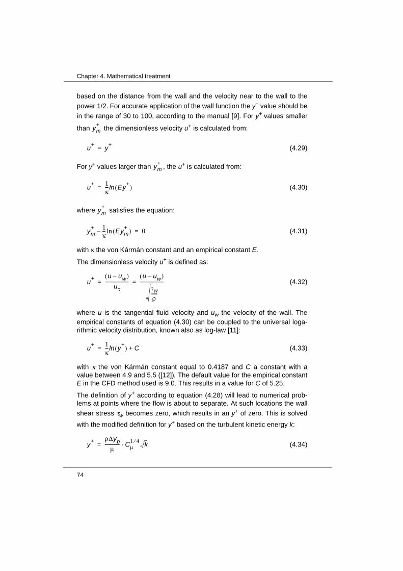
74
Chapter 4. Mathematical treatment
based on the distance from the wall and the velocity near to the wall to the
power 1/2. For accurate application of the wall function the y+ value should be
in the range of 30 to 100, according to the manual [9]. For y+ values smaller
than the dimensionless velocity u+ is calculated from:
(4.29)
For y+ values larger than , the u+ is calculated from:
(4.30)
where satisfies the equation:
(4.31)
with κ the von Kármán constant and an empirical constant E.
The dimensionless velocity u+ is defined as:
(4.32)
where u is the tangential fluid velocity and uw the velocity of the wall. Theempirical constants of equation (4.30) can be coupled to the universal loga-rithmic velocity distribution, known also as log-law [11]:
(4.33)
with κ the von Kármán constant equal to 0.4187 and C a constant with avalue between 4.9 and 5.5 ([12]). The default value for the empirical constantE in the CFD method used is 9.0. This results in a value for C of 5.25.
The definition of y+ according to equation (4.28) will lead to numerical prob-lems at points where the flow is about to separate. At such locations the wall
shear stress τw becomes zero, which results in an y+ of zero. This is solved
with the modified definition for y+ based on the turbulent kinetic energy k:
(4.34)
ym+
u+
y+
=
ym+
u+ 1
κ--- ln Ey
+( )=
ym+
ym+ 1
κ--- Eym
+( )ln– 0=
u+ u uw–( )
uτ---------------------
u uw–( )
τw
ρ------
---------------------= =
u+ 1
κ--- ln y
+( ) C+=
y+ ρ∆yp
µ------------- Cµ
1 4⁄k⋅=

4.4 Two-dimensional test cases
Numerical analysis of a waterjet propulsion system 75
It is assumed that there will always be turbulent fluctuations at a flow separa-tion point, which eliminates the problem.
4.4 Two-dimensional test cases
In order to get an indication of the obtainable accuracy of both themathematical and the numerical methods, the flow around a number of wellknown NACA profiles has been analysed. The flow along isolated profiles aswell as profiles in a cascade have been calculated. For all configurationsexperimental data for the lift and drag is available.
4.4.1 Isolated NACA 0012 profile
The mesh for the numerical analysis of the flow along the NACA 0012 profileis shown in figure 4.1. The chord length of the profile is 600 mm. The domainis divided in three subregions. The first region is meshed with an O-gridaround the profile. This gives good control of the quality of the boundary layercells along the surface. A rectangular box is placed around the first region tomake a transition from the O-grid to an H-grid. In this second region also anO-grid type of mesh is applied.
The third domain extends the numerical domain to either the tunnel walls inthe experiments or to a distance to impose the far-field boundary conditions.At the interface between the second and third domain an arbitrary couplingmethod is employed, which allows non-matching cells at both sides of theinterface.
The O-grid region closest to the profile surface can not be recognised well inthe mesh plot due to the large number of mesh lines. The other two regionscan be distinguished more clearly. In this approach the mesh around theprofiles is identical for all calculated conditions. Regions 1 and 2 can berotated to obtain the desired angle of attack for the profile.
Mesh dependency studies have been carried out to evaluate the variation inlift and drag prediction for an angle of attack of 4 degrees. The number ofcells around the profile and in the direction perpendicular to the profile havebeen varied. The number of cells in the O-grid around the profile has beenvaried from 150 to 330 cells. In the normal direction the number of cells isincreased from 32 to 48. The number of cell in normal direction in the first
region is kept constant to keep a constant y+ value of about 110. This is inaccordance with the requirements for the use of the wall functions.
At the upper and lower boundary of the domain two types of boundaryconditions can be applied: (i) wall boundary conditions or (ii) constantpressure boundary conditions. The first type can be used if the experimentaldata is obtained from wind tunnel tests. The second type is suitable for anunbounded region. For sufficiently large numerical domains both types will

76
Chapter 4. Mathematical treatment
give comparable results. At the inlet boundary a uniform velocity distributionof 10 m/s is prescribed and the constant density of water is used. The
Reynolds number for the calculations becomes . Turbulence intensityis set to 0.01% and the length scale is set to a small fraction of the tunnelheight. All calculations have been carried out with the standard k-ε turbulencemodel and employing wall functions. Solution is based on a second orderMARS (= Monotone Advection and Reconstruction Scheme) discretisationscheme for the momentum equations. This second order method is leastsensitive to the mesh structure and skewness [9]. The k-ε model turbulenceequations are discretised with a first order upwind differencing scheme.
Convergence behaviour of one of the calculated conditions is shown in figure
4.2. The convergence criterion for all calculations is set to 10-4 for themomentum, mass and turbulent kinetic energy equations.
6 106⋅
Figure 4.1 Plot of a part of the mesh as used in calculations of isolated NACA 0012 profile.

4.4 Two-dimensional test cases
Numerical analysis of a waterjet propulsion system 77
Figure 4.3 shows a comparison of the calculated and measured lift and dragfor the isolated NACA 0012 profiles. The experimental data is taken fromAbbott & von Doenhoff [13], where the results of the measurements with
smooth profiles at a Reynolds number of are used. Compressibilityhas been negligible for the tested conditions.
The numerical values for lift and drag are based on the integrated pressureand shear forces acting on the profile surface. The dimensionless lift anddrag coefficients are defined as:
(4.35)
(4.36)
where ρ is the density, v the free-stream velocity and A the surface area ofthe wing, i.e. here the chord length times the width in span wise direction. L isthe lift force and D the drag force.
1.0E-06
1.0E-05
1.0E-04
1.0E-03
1.0E-02
1.0E-01
1.0E+00
1.0E+01
0 50 100 150 200 250
U-velocity residu
V-velocity residu
Mass residu
Turbulent energy residu
Epsilon residu
Figure 4.2 Plot of convergence of a calculation of NACA 0012 profile at angle of attack of 4 degrees for mesh with 222 cells around profile and 40 cells in normal direction.
Iteration number
mass
Res
idua
l
u velocity
v velocity
dissipation
turbulent energy
6 106⋅
clL
12---ρv
2A
-----------------=
cdD
12---ρv
2A
-----------------=
78
Chapter 4. Mathematical treatment
Agreement is good for the lift up to an angle of attack of about 6 degrees. Thecomparison of calculated and measured drag shows a clear over-prediction.The relative error increases from 33% at 0 degrees angle of attack to 55% atan angle of attack of 4 degrees. The deviation between the measurementsand the calculations continuously increases with larger angles of attack.
The results of the mesh sensitivity study are shown in table 4.3 for the liftprediction and in table 4.4 for the drag prediction at an angle of attack of 4degrees. The relative difference in lift coefficient between the minimum andmaximum lift is about 3%. For the drag coefficient a variation of about 9% isfound. The results of the finer meshes do not show a reduction of thedeviation with the experimental data. The error in prediction of drag might berelated to an error in the production term of the turbulence model at thestagnation point, as described by Moore & Moore [14].
0
0.2
0.4
0.6
0.8
1
0 1 2 3 4 5 6 7 8 90
0.01
0.02
0.03
0.04
0.05
cl - EXP
cl - CFD
cd - EXP
cd - CFD
Figure 4.3 Comparison of measured and calculated lift an drag for NACA 0012 profile. Reynolds number of experiments and calculations is 6.0x10⁶. Mesh is based on 222 cells around profile and 32 in normal direction
Section angle of attack [degrees]
c d [-
]
c l [-
]

4.4 Two-dimensional test cases
Numerical analysis of a waterjet propulsion system 79
The sensitivity of the turbulence model is evaluated by a variation of theturbulence intensity of the free stream flow at the inlet boundary condition.Calculations are carried out with a mesh with 222 cells around the profile and32 in normal direction. The level of the turbulence intensity at the inletboundary condition is increased from 0.01% to 1.0%. The results for theprediction of lift and drag coefficient are presented in table 4.5. Variation in liftcoefficient is 4%, whereas the change in drag is about 42%.
The test calculations with the NACA 0012 profile show that the error inprediction of profile drag remains after some mesh refinement steps.Moreover the deviation between experimental data and calculationsincreases significantly when the level of turbulence intensity at the inletboundary increases. It should be noted that the low turbulence levels as usedin the experiments are not representative for the inflow to the waterjet pump.
Table 4.3 Lift coefficient for mesh convergence study. Columnsshow number of cells in normal direction and rows showcells in O-grid around the profile
cl [-] 32 cells 40 cells 48 cells
150 cells 0.4418 0.4386 0.4407
222 cells 0.4384 0.4375 0.4366
330 cells 0.4291 0.4289 0.4302
Table 4.4 Drag coefficient for mesh convergence study. Columnsshow number of cells in normal direction and rows showcells in O-grid around the profile
cd [-] 32 cells 40 cells 48 cells
150 cells 0.010754 0.011324 0.011493
222 cells 0.010522 0.010988 0.011332
330 cells 0.010784 0.011243 0.011495
Table 4.5 Lift and drag coefficients for calculations with variation ofinput values for turbulence intensity
Turbulence intensity [%] cl [-] cd [-]
0.01 % 0.4384 0.010522
0.10 % 0.4287 0.012713
0.50 % 0.4242 0.014147
1.00 % 0.4206 0.014980

80
Chapter 4. Mathematical treatment
It is concluded that with the currently used cell sizes, which is comparablewith the sizes to be used in the three dimensional pump mesh, a significantdeviation between calculated and measured profile drag will remain.
4.4.2 Cascades with NACA 65-410 profiles
Apart from calculations on isolated profiles, also the flow around profiles in acascade have been analysed. Extensive experimental data is available ontests with NACA 65 compressor blade profiles [15]. Data were reported forNACA 65 profiles with various camber lines and a maximum thickness of10% of the chord. Cascades of profiles can be described with two additionalparameters. These are the solidity and the blade angle. The solidity is ameasure for the distance between two profiles in relation to the chord length.The blade angle is defined as the angle between the profile base line and theline connecting all leading edges. An example of the cascade is shown infigure 4.4.Calculations have been carried out for a NACA 65 410 profile with ablade angle of 20 degrees and a solidity of 1.0 and 1.5. The designation ofthe profile is based on a design lift coefficient of 0.4 and a maximumthickness of 10%. The basic camber line used is the a =1.0 mean line (see forexample [13]).
The mesh is created in a similar way as for the isolated NACA 0012 profile.Periodic boundaries are applied to simulate a cascade with an infinite numberof profiles. Turbulence model, discretisation scheme and convergence criteriaare identical to the calculations for the NACA 0012 profile.
Figure 4.4 Geometry of NACA 65-410 cascade. Cascade solidity σ = 1.0, blade angle β = 20 degrees.
β
σ
α

4.4 Two-dimensional test cases
Numerical analysis of a waterjet propulsion system 81
Figure 4.5 shows the non-dimensional pressure distribution Cp for thecascade with a solidity of 1.0 and a blade angle of 20 degree. Thedimensionless pressure Cp coefficient is defined as:
(4.37)
where p is the static pressure, the reference pressure, ρ the density and
the free-stream velocity.
The angle of attack varies from 0.5 to 12.5 degrees. Agreement betweencalculations and measurements is acceptable for most pressure taps for thedifferent conditions.
Lift and drag are derived from the CFD results in the same manner as for theNACA 0012 profile. These results are compared with the experimental data infigure 4.6. The lift is predicted quite well for most conditions. The deviations
Cp
p p∞–
12---ρv∞
2----------------=
p∞
v∞
-1.5
-1
-0.5
0
0.5
1
0 20 40 60 80 100
Experimental values
CFD results-1.5
-1
-0.5
0
0.5
1
0 20 40 60 80 100
Experimental values
CFD results
-1.5
-1
-0.5
0
0.5
1
0 20 40 60 80 100
Experimental values
CFD results
-1.5
-1
-0.5
0
0.5
1
0 20 40 60 80 100
Experimental values
CFD results
Figure 4.5 Pressure coefficient distribution along surface of NACA 65_410 profile for different angles of attack. Cascade solidity = 1.0, blade angle = 20 degrees.
α = 0.5 degrees α = 4.5 degrees
α = 12.5 degreesα = 8.5 degrees
Chord length [%] Chord length [%]
Chord length [%]Chord length [%]
Cp
[-]
Cp
[-]
Cp
[-]
Cp
[-]

82
Chapter 4. Mathematical treatment
between the measured and calculated drag vary between about 10% and50%. This is in agreement with the results of the isolated NACA 0012 profile.
It can be concluded that the trend of over-prediction of drag occurs for bothisolated profiles as well as for profiles in a cascade. In both cases the lift ispredicted much better. In the next subsection the consequences of an error inlift or drag on the prediction of thrust and torque are discussed.
4.4.3 Sensitivity of errors in drag on thrust and torque
Torque and thrust of a waterjet impeller are related to the tangential and axialforce experienced by the blade sections. These forces can be derived fromthe lift and drag of these profiles. Consequently, if the blade profile drag isover-predicted, there will be an effect on the prediction of the torque and thethrust. Lift and drag are transformed into axial and tangential forces with:
(4.38)
where φ is the inflow angle, L the lift force and D the drag force. The inflowangle φ is related to the blade angle β and the angle of attack α of the flowwith respect to the chord line:
(4.39)
Figure 4.6 Comparison of measured and calculated lift and drag for NACA 65_410 profiles in cascade with solidity of 1.0 and blade angle of 20 degrees.
-0.2
-0.1
0
0.1
0.2
0.3
0.4
0.5
0.6
0.7
0.8
-4 0 4 8 12 16 20
-0.02
-0.01
0
0.01
0.02
0.03
0.04
0.05
0.06
0.07
0.08
cl - exp
cl - CFD
cd - exp
cd - CFD
Angle of attack [degrees]
c d [-
]
c l [-
]
Fax φ L⋅cos φ D⋅sin–=
Ftan φ L⋅sin φ D⋅cos+=
φ β α–=

4.4 Two-dimensional test cases
Numerical analysis of a waterjet propulsion system 83
The drag prediction based on CFD calculations can be expressed as:
(4.40)
where ε represents the relative over-prediction of the profile drag. It isassumed that:
(4.41)
This can be up to about 50%. Figure 4.7 shows a sketch of the forces actingon a profile. From this sketch the effect of a higher drag can already berecognised.
Substitution of equation (4.40) in equation (4.38) gives an expression for theaxial and tangential force prediction based on CFD results.These forces canbe related to the exact solutions to determine the resulting relative error inaxial and tangential direction. The relative error for the axial force can becalculated with:
(4.42)
where φ is the inflow angle, L/D is the lift over drag ratio. The relative error intangential direction yields:
(4.43)
DCFD Dexact 1 ε+( )=
LCFD Lexact=
Figure 4.7 Sketch of forces acting on profile
∆torque
∆drag
∆thrustφ
α β
Fax_CFD
Fax_exact----------------------- 1
ε1
φtan------------
Lexact
Dexact----------------⋅ 1–
------------------------------------------–=
Ftan_CFD
Ftan_exact------------------------ 1
ε
φtanLexact
Dexact----------------⋅ 1+
------------------------------------------+=

84
Chapter 4. Mathematical treatment
To get an indication of the influence of the error in drag prediction on the axialand tangential force, the data for the NACA 65-410 cascade will be used. Thelift over drag ratio as function of the angle of attack is derived from figure 4.6.The relative errors in axial and tangential force are plotted as function of theangle of attack in figure 4.8. The drag over-prediction is set to 20%, 40% and60%.
From this diagram is becomes clear that the effect on axial force is very smalleven for large over-prediction of drag. The estimated error on thrust will beless than 1% for most cases. On the other hand the error in tangential forceremains significant for realistic values of the angle of attack α and drag errorfactor ε. The error in tangential force can be about 2.0 to 8.0%. For cascadeswith smaller blade angles β, the error in tangential force will increase evenmore.
It is to be expected that this effect will be noticeable in both impeller andpropeller torque calculations. Calculation of thrust seems to be insensitive toan error in drag. It is expected that the calculation of pump head shows thesame behaviour, based on the similarity between propeller thrust and pumphead as shown in equation (2.34).
-2%
-1%
0%
1%
2%
3%
4%
5%
6%
7%
8%
9%
10%
11%
12%
0 2 4 6 8 10 12 14 16 18
-
-
Figure 4.8 Relative errors in tangential and axial forces due to over-prediction of profile drag. Data is based on NACA 65-410 cascade with solidity of 1.0 and blade angle of 20 degrees.
Angle of attack [degrees]
FC
FD
/Fex
act [
-]
Tangential force error - ε=0.20Tangential force error - ε=0.40Tangential force error - ε=0.60Axial force error - ε=0.20Axial force error - ε=0.40Axial force error - ε=0.60

4.5 Nomenclature
Numerical analysis of a waterjet propulsion system 85
4.5 Nomenclature
A area m2
cd drag coefficient -
cl lift coefficient -
Cp pressure coefficient -
D drag N
F force N
g gravitational acceleration m/s2
k turbulent kinetic energy m2/s2
L lift force N
lmix Prandtl’s mixing length m
P production term of turbulence m3/s2
p pressure N/m2
Re Reynolds number -
t time s
u+ dimensionless velocity -
v velocity m/s
∆yp distance from wall m
y+ dimensionless wall distance -
z coordinate in vertical direction m
Greek symbols
α angle of attack degrees
β blade angle degrees
ε dissipation m2/s3
ε relative error in drag prediction -
φ inflow angle degrees
κ Von Kármán constant -
µ dynamic viscosity kg/ms
ρ fluid density kg/m3
τw wall shear stress N/m2
ω vorticity, dissipation rate 1/s
Subscripts
ax axial direction

86
Chapter 4. Mathematical treatment
CFD based on CFD results
eff effective (=laminar + turbulent)
exact based on exact formulations
i,j directions
imp impeller
inl inlet
T turbulent
tan tangential direction
tip impeller blade tip
w wall
x,y,z carthesian coordinate system directions
Superscripts
v’ fluctuating part
v time averaged value
4.6 References
[1] Aungier, R.H.,’Centrifugal compressors’, ASME Press, New York, 2000
[2] Van Esch, B.P.M.,’Simulation of three-dimensional unsteady flow inhydraulic pumps’, PhD thesis, University of Twente, 1997
[3] Van Os, M.J.,’On the flow and cavitation inception of mixed-flow impel-lers’, PhD thesis, University of Twente, 1998
[4] Kunz, R.F., Lakshminarayana, B., Basson, A.H., ‘Investigation of tipclearance phenomena in an axial compressor cascade using Euler andNavier-Stokes procedures’, Journal of Turbomachinery, Vol 115, pp453-467, 1993
[5] Goto, A.,’Study of internal flows in a mixed-flow pump impeller at vari-ous tip clearances using three-dimensional viscous flow computations’,Journal of Turbomachinery, Vol 114, pp 373-382, 1992
[6] Fox, R.W., McDonald, A.T.,’Introduction to fluid mechanics’, Third Edi-tion, John Wiley & Sons, New York, 1985
[7] Wilcox, D.C.,’Turbulence modeling for CFD’, Griffin Printing, Glendale,1993
[8] Ferziger, J.H., Peric, M., ‘Computational methods for fluid dynamics’,Second edition, Springer, Berlin, 1999

4.6 References
Numerical analysis of a waterjet propulsion system 87
[9] Computational Dynamics Limited, ‘Star-CD methodology, version3.150’, 2001
[10] Versteeg, H.K., Malalasekera, W., ‘An introduction to ComputationalFluid Dynamics’, Longman Scientific & Technical, Essex, 1995
[11] Schlichting, H., ‘Boundary layer theory’, McGraw-Hill, New York, 1968
[12] Cebeci, T., Smith, A.M.O., ‘Analysis of turbulent boundary layers’, Aca-demic press, New York, 1974
[13] Abbott, I.H., Von Doenhoff, A.E. ,’Theory of wing sections’, Dover Pub-lications, Inc., New York, 1958
[14] Moore, J.G., Moore, J., ‘Controlling over-production of turbulence intwo-equation models by limiting the anisotropy of the Reynolds normalstresses’, 1997 ASME Fluids Engineering Division Summer Meeting,1997
[15] Emery, J.C., Herrig, L.J., Erwin, J.R., Felix, A.R., ‘Systematic two-dimensional cascade tests of NACA 65-series compressor blades atlow speeds’, NACA report 1368, Langley Aeronautical Laboratory, Lan-gley Field, 1958

88
Chapter 4. Mathematical treatment

Numerical analysis of a waterjet propulsion system 89
Chapter 5 Numerical analysis of waterjet inlet flow
In this chapter the flow through the waterjet inlet will be analysed in moredetail. First a critical review of several published analyses of the flow throughwaterjet inlets will be given, which provides additional information about thesuitable numerical approach for the inlet flow CFD analysis. Discussion of theapplication of the numerical method is divided into two parts: (i) the meshgeneration for the three dimensional inlet geometry based on theexperimental set-up for the finite volume analysis and (ii) the selection ofboundary conditions. In order to validate the computational method the CFDresults are compared with experimental data for a model scale waterjet inletduct. During the validation process, the effects of the confinement of the flowdue to the cavitation tunnel walls are also addressed.
The CFD results can be used to visualise the flow behaviour in more detail.Besides pressure and velocity distribution, it is also interesting to quantifywall friction and to determine the shape of the dividing streamtube.
5.1 Review of CFD analyses on waterjet inlets
Calculations for a three dimensional waterjet inlet have been reported byFørde et al. [1]. For the calculations an Euler method was employed, butcomputed results were not validated with measurements. The presentedvelocity distribution at the impeller plane is not in agreement with a typicalflush type waterjet inlet. This is caused by the neglect of the boundary layervelocity profile at the inlet and absence of viscous effects in the method,

90
Chapter 5. Numerical analysis of waterjet inlet flow
necessary for describing the development of the boundary layer in the inletduct.
A potential flow method has been applied by Van Terwisga [2]. Comparison ofthe calculated pressure distribution along the ramp and the cutwater (or inletlip) with experimental data shows large deviations. This is due to the neglectof viscous losses and due to small deviations in the calculated velocity fieldnear the stagnation point at the cutwater. A small deviation of the angle ofattack at the cutwater can lead to relatively large differences in the predictionof the static pressure distribution.
Pylkkänen ([3], [4]) presented results of CFD calculations obtained from aRANS code. A two-dimensional model of a waterjet inlet is used for theseanalyses. Differences between calculations and measurements of pressureare about 11 to 15%. The experimental data is based on measurements of athree-dimensional inlet on a windtunnel. It is known that an actual three-dimensional waterjet inlet ingests water from a region that is wider than theinlet itself. In a two-dimensional situation this phenomenon cannot bereproduced, and therefore the pressure distribution at the lip section will bedifferent. In the second part of the inlet, the rectangular cross-sectiontransitions to a circular cross-section in general. This transition is not takeninto account in a two-dimensional analysis either. Therefore it is expected thatthe pressure distribution in this part of the inlet will show a deviation from thethree-dimensional case as well.
The necessity of considering the three-dimensional geometry is shown byVan der Vorst et al. [5]. Calculations were made for a two and for a three-dimensional case. Results of both calculations were compared withexperimental data. The calculated pressure distribution along the inlet rampcentre line shows agreement with the measurements for the three-dimensional analysis, whereas large deviations are found for the results ofthe calculations of the two-dimensional geometry. The pressuremeasurements were performed for a model scale waterjet inlet, mounted ontop of a windtunnel.
Another example of the use of viscous methods for the calculation of three-dimensional inlet flows was reported by Seil et al. [6]. In these calculations,the geometry of the pump is included. The effect of the impeller is modelledwith an actuator disk, however. Calculated results show that the location ofthe stagnation point at the cutwater depends on the IVR value. It is also foundthat the level of non-uniformity of the velocity profile at the bend increaseswith increasing IVR. This non-uniformity vanishes towards the impeller plane,where the actuator disk is located. This behaviour may be a result of theimplementation of the actuator disk. Yang et al. [7] have also calculated theflow around a waterjet inlet with a viscous flow method. A complete hull isincluded in the computational domain. Agreement between measurementsand CFD results is poor for the pressure distribution along the ramp and lipcentre lines.
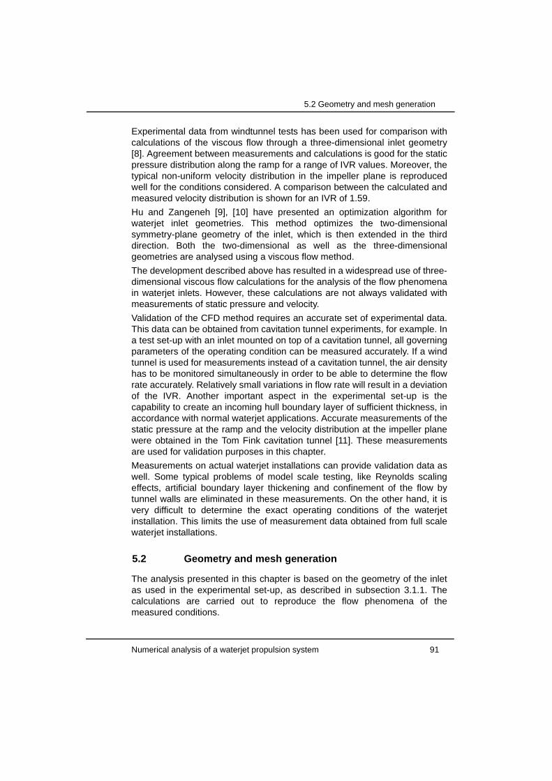
5.2 Geometry and mesh generation
Numerical analysis of a waterjet propulsion system 91
Experimental data from windtunnel tests has been used for comparison withcalculations of the viscous flow through a three-dimensional inlet geometry[8]. Agreement between measurements and calculations is good for the staticpressure distribution along the ramp for a range of IVR values. Moreover, thetypical non-uniform velocity distribution in the impeller plane is reproducedwell for the conditions considered. A comparison between the calculated andmeasured velocity distribution is shown for an IVR of 1.59.
Hu and Zangeneh [9], [10] have presented an optimization algorithm forwaterjet inlet geometries. This method optimizes the two-dimensionalsymmetry-plane geometry of the inlet, which is then extended in the thirddirection. Both the two-dimensional as well as the three-dimensionalgeometries are analysed using a viscous flow method.
The development described above has resulted in a widespread use of three-dimensional viscous flow calculations for the analysis of the flow phenomenain waterjet inlets. However, these calculations are not always validated withmeasurements of static pressure and velocity.
Validation of the CFD method requires an accurate set of experimental data.This data can be obtained from cavitation tunnel experiments, for example. Ina test set-up with an inlet mounted on top of a cavitation tunnel, all governingparameters of the operating condition can be measured accurately. If a windtunnel is used for measurements instead of a cavitation tunnel, the air densityhas to be monitored simultaneously in order to be able to determine the flowrate accurately. Relatively small variations in flow rate will result in a deviationof the IVR. Another important aspect in the experimental set-up is thecapability to create an incoming hull boundary layer of sufficient thickness, inaccordance with normal waterjet applications. Accurate measurements of thestatic pressure at the ramp and the velocity distribution at the impeller planewere obtained in the Tom Fink cavitation tunnel [11]. These measurementsare used for validation purposes in this chapter.
Measurements on actual waterjet installations can provide validation data aswell. Some typical problems of model scale testing, like Reynolds scalingeffects, artificial boundary layer thickening and confinement of the flow bytunnel walls are eliminated in these measurements. On the other hand, it isvery difficult to determine the exact operating conditions of the waterjetinstallation. This limits the use of measurement data obtained from full scalewaterjet installations.
5.2 Geometry and mesh generation
The analysis presented in this chapter is based on the geometry of the inletas used in the experimental set-up, as described in subsection 3.1.1. Thecalculations are carried out to reproduce the flow phenomena of themeasured conditions.

92
Chapter 5. Numerical analysis of waterjet inlet flow
The geometry of a waterjet inlet duct can be described by a number ofparameters, e.g. the pump inlet diameter, the inlet angle, the radius ofcurvature of the bend and the shape of the cutwater. It is therefore convenientto develop a fully parametric three-dimensional geometry and meshgenerator, based on a list of geometric parameters. Figure 5.1 shows asketch of a two-dimensional inlet geometry with the main parameters. Basedon the geometric parameters the three-dimensional shape of the inlet iscalculated. This geometrical data is used in the CFD pre-processor. From thisinput data the block definitions are created. The topology of the blocks is keptidentical for all waterjet inlets. Figure 5.2 shows a typical output of the usedblock structure. A thin layer of cells is created at the walls of the inlet, in order
RAMP RADIUS
TRANSITION LENGTH
CYLINDRICAL LENGTH
BENDING RADIUS
SHAFTDIAMETER
INLETANGLE
TRANSITION ANGLE
DIAMETERINLET
SHAFTDIAMETER
RAMP
POINTTANGENCY
CUTWATER
Figure 5.1 Inlet geometry with main parameters and specific nomenclature listed
Figure 5.2 Wire frame plot of block structure of the inlet mesh
5.2 Geometry and mesh generation
Numerical analysis of a waterjet propulsion system 93
to get high quality cells in the boundary layer. The averaged y+ value of thecells near the wall is about 60 for this mesh.
Near the so-called cutwater (or inlet lip), a local refinement of the mesh isapplied to capture the gradients of the flow field better. The final mesh isshown in figure 5.3a and in figure 5.3b a detail of the cutwater with localrefinement and the region around the shaft is shown. In case of computations
Figure 5.3a Final mesh of waterjet inlet (half of the complete domain)
Figure 5.3b Detail of cutwater mesh with local refinement and regular meshcoupling on the block boundaries (left) and mesh around the (stationary) shaft

94
Chapter 5. Numerical analysis of waterjet inlet flow
with a stationary shaft or without a shaft, the computational domain isrestricted to half the geometry for reasons of symmetry with respect to thevertical plane through the centreline of the pump.
5.3 Numerical approach
5.3.1 Boundary conditions
All cell faces at the boundary of the computational domain require some typeof boundary condition.
At the inlet of the computational domain an inlet type boundary condition isapplied. This type of boundary condition requires a prescription of thevelocities in all three directions and values for the turbulence intensity and thelength scale, if a turbulence model is used. The velocity profile, whichrepresents the hull boundary layer, is input through a user-routine. In thisroutine a power-law velocity profile is calculated for all cells that are located inthe boundary layer. The presented calculations are based on a boundarylayer profile with a power-law value n=7 and a thickness δ of 0.3D, with D thediameter of the inlet. An undisturbed uniform velocity is prescribed in theremainder of the cells. The turbulence intensity is set to 2.0% and the lengthscale to 0.05 m, which is equivalent to about 8% of the tunnel inlet hydraulicdiameter.
At the impeller plane the total mass flow leaving the domain through the inletduct is imposed. This is established with a fixed flow outlet boundarycondition. This type of condition allows for a non-uniform velocity distributionover the surface. The pressure distribution in the outflow plane is part of thesolution as well.
For the outflow plane of the cavitation tunnel a constant pressure boundarycondition is used. It is assumed that the static pressure is uniform at largeenough distance from the waterjet inlet. The resulting velocity distribution willbe non-uniform, however.
The side plane and the bottom plane of the domain are placed at the locationof the cavitation tunnel walls. For these walls, the slip condition is applied asthe wall boundary condition. The mesh near these walls can be maderelatively coarse, since the boundary layer is not resolved. With this boundarycondition the normal velocity is set to zero, which simulates the effect of thewall on the flow. The effects of the development of the natural tunnel wallboundary layer, characterised by the displacement and momentum thickness,are neglected. The effects of the actual boundary layer in the cavitation tunnelare analysed during the tests and it is concluded that the effect of blockagewas less than 0.2%.
For conventional waterjet inlet CFD analyses the tunnel walls are not takeninto account. The side and bottom planes of the domain are modelled as

5.3 Numerical approach
Numerical analysis of a waterjet propulsion system 95
constant pressure planes. Using pressure boundary conditions, additionalinflow of water is allowed. The difference between wall boundary conditionsand constant pressure boundary conditions is investigated later on in thisthesis.
Calculations for a half model geometry require symmetry conditions at thesymmetry plane. If the complete model is analysed with shaft rotation, anadditional wall boundary condition is applied to the shaft surface in order tomodel the rotation.
5.3.2 Fluid properties
Selection of the fluid properties for the waterjet inlet analysis isstraightforward. As discussed in the previous chapter, the flow can beconsidered as incompressible, which results in a constant density. All model
scale calculations have been carried out with a density ρ of 1000 kg/m3. Thedynamic fluid viscosity µ is set to 0.001 kg/ms.
Turbulent flow behaviour is modelled with a turbulence model. Though theCFD method provides several different turbulence models with differentlevels of complexity, the well established high-Reynolds number flow k-εturbulence model is applied for all calculations. This also implies the use ofwall functions to impose the no-slip boundary condition. It is acknowledgedthat the standard k-ε turbulence model has a moderate performance for sometypes of flow. These are (i) some external unconfined flows, (ii) flows withlarge extra strains (e.g. the flow in curved boundary layers, swirling flows), (iii)rotating flows and (iv) fully developed flows in non-circular ducts, see [12].Results from the validation process will show whether the choice of thisturbulence model for the present flow is acceptable.
The effect of gravity is accounted for in the analyses, but it should bementioned that this is only an additional post-processing feature, since thedensity is constant.
5.3.3 Discretisation and solution algorithm
Solution of the partial differential equations requires a discretisation scheme.As for the turbulence models, several methods are provided within the CFDmethod used. Here all calculations have been performed employing thesecond order MARS scheme (short for Monotone Advection andReconstruction Scheme) for the momentum equations. This second ordermethod is least sensitive to the mesh structure and skewness [13]. The k-εmodel turbulence equations are discretised with a first order upwinddifferencing (UD) scheme.
The coupling between the velocity and pressure field is resolved with aniterative solution strategy based on the SIMPLE pressure-correction method.

96
Chapter 5. Numerical analysis of waterjet inlet flow
In this algorithm, originally put forward by Patankar and Spalding [14], theconvective fluxes are evaluated from an estimated velocity field. Furthermore,an estimation for the pressure distribution is used to solve the momentumequations. The continuity equation then yields a pressure correctionequation, which yields a pressure correction field. This pressure correctionterm is used in turn to update the estimated velocity and pressure field. Thisprocess is iterated until the velocity and pressure fields are converged.
The system of discretised partial differential equations is solved with anAlgebraic MultiGrid (AMG) algorithm.
Figure 5.4 shows the convergence behaviour of a calculation for an IVR of1.87. In order to accelerate the convergence, first 125 iterations are carriedout with the first order UD scheme for the velocity components. The restartwith MARS discretisation causes the step in the residuals of the momentum
and the mass. The convergence criterion is set to 10-4 for the momentum,mass and turbulent kinetic energy equations.
5.4 Validation with experimental data
The experimental data used in this chapter is measured at the Tom Finkcavitation tunnel [11] as described in subsection 3.1.1. In this test programmeasurements are made on two different inlet geometries. The experimentalprogram consists among others of static pressure measurements along the
1.0E-06
1.0E-05
1.0E-04
1.0E-03
1.0E-02
1.0E-01
1.0E+00
1.0E+01
0 50 100 150 200 250 300
U-velocity
V-velocity
W-velocity
Mass
Turbulent energy
Dissipation
Figure 5.4 Plot of convergence of a calculation of waterjet inlet flow phenomena for IVR = 1.87.
Iteration number
Res
idua
l
mass
u velocity v velocity
dissipation
turbulent
w velocity
energy

5.4 Validation with experimental data
Numerical analysis of a waterjet propulsion system 97
ramp centre line, total pressure measurements at the plane just upstream ofthe impeller, cavitation inception observations at the cutwater andvisualisation of streamlines. In the following sections, measured data will beused for comparisons with CFD results.
5.4.1 Comparison of static pressure along the ramp centre line
The static pressure is measured at the ramp centre line at 12 differentlocations. The locations are determined by the distance along the rampcentre line from the impeller plane towards the entrance of the inlet. Theentrance of the inlet, sometimes denoted as ramp tangency point, is locatedat a distance of 1000 mm for this model scale inlet.
The static pressure is made non-dimensional using the density ρ and thetunnel speed vtunnel:
(5.1)
The reference static pressure pref and the tunnel speed are taken at alocation upstream of the inlet, since the velocity, and the pressuredownstream of the inlet vary with the value of IVR value (see equation(2.12)).
The static pressure is measured for eight different IVR values. Table 5.1shows the conditions, used for the measurements. The Reynolds numberReinl is defined in equation (4.2).
Table 5.1 Parameters of measured conditions for the static pressuredistributions. Dinlet = 150 mm.
IVR [-](=vtunnel/vpump)
vtunnel[m/s]
vpump[m/s]
Reinl [-]
1.07 8.00 7.48 11.21 x 10⁵
1.21 8.00 6.61 9.92 x 10⁵
1.29 8.00 6.20 9.30 x 10⁵
1.50 8.00 5.33 8.00 x 10⁵
1.70 8.00 4.71 7.06 x 10⁵
1.87 8.00 4.28 6.42 x 10⁵
2.03 8.00 3.94 5.91 x 10⁵
2.19 8.00 3.65 5.48 x 10⁵
Cp
p pref–
12---ρvtunnel
2-----------------------=

98
Chapter 5. Numerical analysis of waterjet inlet flow
-0.3
-0.2
-0.1
0
0.1
0.2
0.3
0.4
0.5
0 200 400 600 800 1000 1200
ExperimentsCFD
IVR = 1.21IVR = 1.50IVR = 1.87IVR = 2.19
-0.3
-0.2
-0.1
0
0.1
0.2
0.3
0.4
0.5
0 200 400 600 800 1000 1200
ExperimentsCFD
IVR = 1.07IVR = 1.29IVR = 1.70IVR = 2.03
Figure 5.5 Comparison of measured and calculated pressure coefficient Cp along the ramp centre line. Values are given as a function of the distance from the impeller plane. The data for different values of IVR are divided in 2 groups for improved visibility.
Distance along ramp [mm]
Cp
[-]
Distance along ramp [mm]
Cp
[-]

5.4 Validation with experimental data
Numerical analysis of a waterjet propulsion system 99
The comparison with CFD results is shown in figure 5.5. Values of pressurecoefficient Cp along the ramp centre line are given as function of the distancefrom the impeller plane. The two diagrams present the data for alternatevalues of IVR.
Both figures show a good agreement between measurements and CFDcalculations along the entire ramp section. The discontinuity in calculatedpressure between 350 mm and 400 mm is due to the presence of the shaft.This influence is strongest at low IVR since the velocity in the inlet duct isthen highest. The static pressure at the impeller plane increases withincreasing IVR (due to decreasing vpump) according to the expectations.However, at high IVR values the static pressure is more or less constant. Thisis due to increased non-uniformity and hydraulic losses.
Figure 5.6 shows the pressure distribution in the symmetry plane of theconfiguration for an IVR of 1.07 (top) and 2.03 (bottom). It can be observedthat the effect of IVR on the pressure distribution is not restricted to the ramp.Clear differences in pressure can be recognized at the cutwater and in thebend of the inlet.
From the pressure distributions can be seen that the location of thestagnation point at the cutwater changes with variation of IVR. As aconsequence, the location of minimum value of the pressure also changes.This phenomenon is reported before by Seil [6]. It is shown in more detail infigure 5.7, where the pressure distribution along the cutwater is presented forall calculated IVR conditions. On the left part of the diagram the negative scoordinates represent the lower part of the cutwater, whereas the positive scoordinates represent the upper part of the cutwater. The influence of IVR onthe results can be recognised clearly. The stagnation point moves from anegative s coordinate in the positive direction for increasing IVR. Thelocations of the minimum pressure can be divided in two groups. For IVRconditions up to 1.29 the minimum pressure is found at a location withpositive s coordinate. For higher IVR, the location of minimum pressure isfound at a negative s coordinate.
The movement of the stagnation point, and consequently the location of theminimum pressure, is related to the change in the shape of the dividingstreamtube with varying IVR. The streamtube analysis will be given in section5.5.
Analysis of the pressure in 5.7 learns that the static pressure at the tunneloutlet plane is not equal to the reference pressure at the inlet plane andmoreover, this variation is dependent on IVR. This deviation in static pressuremight influence the experimental determination of the cavitation inceptionpressure, when the location of the minimum pressure is at the lower side (orhull side) of the inlet for high IVR conditions. The cavitation inception resultswill be compared with CFD results in the next section.

100
Chapter 5. Numerical analysis of waterjet inlet flow
Figure 5.6 Pressure coefficient Cp at symmetry plane for IVR of 1.07 (top) and IVR of 2.03 (bottom).

5.4 Validation with experimental data
Numerical analysis of a waterjet propulsion system 101
5.4.2 Comparison of cavitation inception pressure at cutwater
Cavitation below the cutwater occurs at high IVR conditions. For four IVRvalues the inception pressure is determined by visual observation. During thetests the reference pressure pref in the tunnel is gradually reduced until asmall cavity is observed. With this procedure only cavities at the lower side ofthe cutwater could be observed. These are typical for high IVR conditions.The measuring point for the reference pressure pref is located upstream ofthe inlet at half the tunnel height, as shown in figure 3.1 on page 50.
The cavitation inception pressure is presented in non-dimensional form,according to:
(5.2)
where pv is the vapour pressure of the fluid, h the height correction betweenthe cutwater and the centre plane of the cavitation tunnel and vpump theaverage axial inflow velocity of the pump. The comparison of theexperimental results and the CFD results is shown in figure 5.8.
-2.5
-2
-1.5
-1
-0.5
0
0.5
1
1.5
-100 -80 -60 -40 -20 0 20 40 60 80 100
IVR = 1.07
IVR = 1.21
IVR = 1.29
IVR = 1.50
IVR = 1.70
IVR = 1.87
IVR = 2.03
IVR = 2.19
Distance s along cutwater [mm]
Cp
[-]
IVR=1.07
IVR=1.07
IVR=2.19
IVR=2.19
s<0
s>0
s=0
Figure 5.7 Calculated pressure coefficient Cp along the cutwater for different IVR values. Negative s coordinate represents lower side of cutwater and positive coordinate represents upper side.
σv_pump
pref pv– ρgh–
12---ρvpump
2--------------------------------------=

102
Chapter 5. Numerical analysis of waterjet inlet flow
It should be noted that the pump inflow velocity is used in the definition ofσv_pump, whereas the ship speed is used for Cp. With the current σ definitionthe inception behaviour of different inlet geometries at high IVR can beevaluated better.
Agreement between experiments and CFD calculations is good for all fourtested conditions. The calculated conditions at lower IVR values show theexpected behaviour. At a certain IVR the dividing streamline is optimallyaligned with the cutwater geometry, which results in a minimum value forσv_pump. Further decrease of IVR results in the point of minimum pressure,i.e. the cavitation inception point, moving to the inner side of the inlet.
Effect of tunnel walls
At normal waterjet operating conditions cavitation inception occurs below thecutwater in general. Figure 5.7 shows that the pressure in this region is notconstant and depends on IVR. This is due to the effect of tunnel walls andconservation of mass in the complete system. The mass flow which entersthe tunnel is split into a part which leaves the domain through the waterjetinlet and a part which leaves through the tunnel exit section. As long as thepump exit is open the mass flow rate at the exit of the tunnel section is lowerthan at the inlet. Because the tunnel cross-section is constant, this results in
0
1
2
3
4
5
6
7
1 1.2 1.4 1.6 1.8 2 2.2 2.4
Measurements
CFD calculations
Figure 5.8 Comparison of measured and calculated cavitation inception at cutwater
IVR [-]
σ v_p
ump
[-]

5.4 Validation with experimental data
Numerical analysis of a waterjet propulsion system 103
lower velocities and consequently a higher static pressure. The pressureincrease as a function of IVR can be estimated as:
(5.3)
where Apump is the cross-sectional area at the impeller plane and Atunnel thecross-sectional area of the tunnel. The effect of viscous losses is neglected inthis estimation.
The diameter of the cross-sectional area at the impeller plane is 150 mm andthe cavitation tunnel has a square section of 600 x 600 mm. The velocity atthe outlet of the tunnel shows a drop of about 5% for an IVR = 1.0 to 2% forIVR = 2.0. Figure 5.9 shows the pressure difference ∆Cp based on the CFDresults and the theoretical value. Agreement between the analytical valueand the numerical result is good over the complete IVR range.
Equation (5.3) neglects the effect of the displacement thickness of theboundary layer on the tunnel walls in the calculation of the mass fluxes.Inclusion of this displacement thickness will result in a slightly lower massflow entering the tunnel section, which is equivalent to a lower IVR. Theanalytical pressure difference estimate will increase with less than onepercent in this case. This simplification is assumed to be justified. Moreover,hydraulic losses in the tunnel are not taken into account in the estimation.These hydraulic losses will reduce the actual pressure increase in the tunnel.However, for a first indication of the effect of the confinement of the tunnel
∆Cp
2Apump
IVR Atunnel⋅----------------------------------
Apump
IVR Atunnel⋅----------------------------------
2–=
0
0.01
0.02
0.03
0.04
0.05
0.06
0.07
0.08
0.09
0.1
1 1.2 1.4 1.6 1.8 2 2.2 2.4
CFD
Equation (5.3)
Figure 5.9 Dimensionless pressure increase in tunnel section based on CFD results and analytical formula
IVR [-]
∆Cp
[-]

104
Chapter 5. Numerical analysis of waterjet inlet flow
walls on the pressure distribution, equation (5.3) can be used as a firstestimate.
In actual conditions at open sea the equivalent cross sectional area goes toinfinity and consequently the pressure difference tends to zero. This is inaccordance with the expectations.
Effect of the tunnel walls on static pressure distribution along the ramp isshown in figure 5.10 for two IVR values. These are the same conditions asshown in the symmetry plane pressure distributions of figure 5.6. Cleardeviations between the calculation with and without the walls can be seen inthe first part of the inlet. In this region the pressure is influenced most by thelocal tunnel pressure. Moreover, the deviations are larger for the low IVRcondition. This is in line with equation (5.3). Further downstream in the inletduct the pressure distribution is similar for both configurations.
It is to be expected that the largest influence of the tunnel pressure increase,due to the wall confinement, is found in the tunnel downstream of thecutwater. This is the location where the cavitation inception occurs at mediumand at high IVR. The effect of the tunnel walls on cavitation inceptionpressure is shown in figure 5.11. The deviations between the two series ofcalculations are large. For a cavitation free design, the cavitation inceptiondiagram of the inlet is matched with the available ambient pressure. Thecavitation inception diagram represents the required pressure to avoidcavitation. As long as the required pressure is lower than the availableambient pressure, cavitation free operation is possible. Figure 5.11 showsthat the required pressure, based on experiments or calculations with tunnel
-0.3
-0.2
-0.1
0
0.1
0.2
0.3
0.4
0.5
0 200 400 600 800 1000 1200
IVR = 1.07 - wall
IVR = 1.07 - no wall
IVR = 2.03 - wall
IVR = 2.03 - no wall
Inlet geometry
Figure 5.10 Comparison of calculations of static pressure distribution along ramp for configuration with and without tunnel walls
Distance along ramp [mm]
Cp
[-]

5.4 Validation with experimental data
Numerical analysis of a waterjet propulsion system 105
walls is too optimistic for medium and high IVR. The actual required pressureis higher, as can be seen from the calculations without tunnel walls. Thiseffect should always be taken into consideration when interpreting cavitationinception results in a test set-up with finite dimensions.
5.4.3 Comparison of total pressure at impeller plane
Good agreement between measurements and calculations is shown in theprevious subsections for the static pressure along the ramp and the cavitationinception that occurs at the cutwater. In this subsection the total pressuredistribution in the impeller plane is evaluated. The impeller plane is defined asthe cross-sectional area at the end of the inlet, just upstream of the impeller,as shown in figure 3.1.
Total pressure measurements have been made with a pitot-rake positioned atdifferent radii. In the tangential direction steps of 10 degrees are madebetween the measurement locations.
Figures 5.12a to 5.12d show the comparison between the measured and thecalculated total pressure distribution for four different IVR conditions. Thelowest IVR is a normal operating condition of 1.68 and the highest IVR is avery high speed condition of 2.19. The other two IVR conditions are inbetween with values of 1.87 and 2.03. The results are made non-dimensionalwith the tunnel speed in a similar way as the static pressure, i.e.:
0
1
2
3
4
5
6
7
1 1.2 1.4 1.6 1.8 2 2.2 2.4
Measurements
CFD with tunnel walls
CFD without tunnel walls
Figure 5.11 Comparison of calculations of cavitation inception pressure for configuration with and without tunnel walls
IVR [-]
σ [-
]
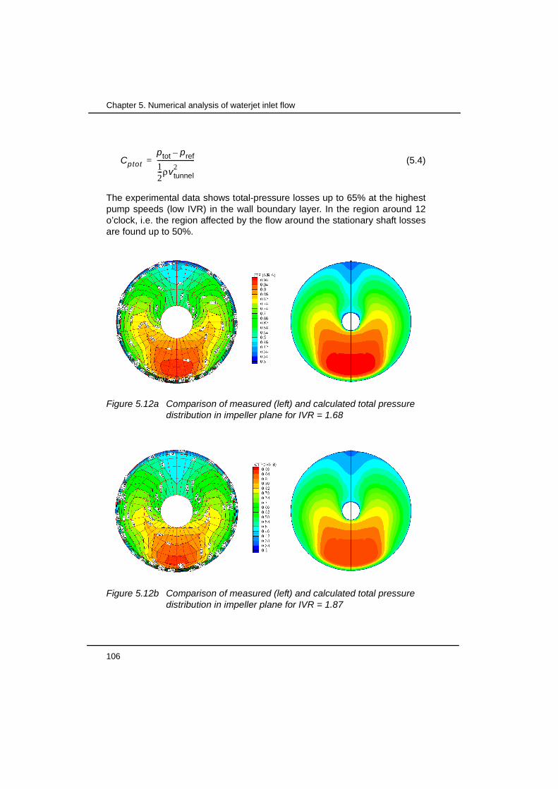
106
Chapter 5. Numerical analysis of waterjet inlet flow
(5.4)
The experimental data shows total-pressure losses up to 65% at the highestpump speeds (low IVR) in the wall boundary layer. In the region around 12o’clock, i.e. the region affected by the flow around the stationary shaft lossesare found up to 50%.
Cptot
ptot pref–
12---ρvtunnel
2------------------------=
Figure 5.12a Comparison of measured (left) and calculated total pressure distribution in impeller plane for IVR = 1.68
Figure 5.12b Comparison of measured (left) and calculated total pressure distribution in impeller plane for IVR = 1.87

5.4 Validation with experimental data
Numerical analysis of a waterjet propulsion system 107
For all four conditions the qualitative agreement between the measurementsand the calculations is good. The typical distribution and the effect of the shaftis reproduced well within the CFD model. It appears that the computedboundary layer is thinner than in the experiment. However, measuring with atotal pressure tube close to the wall will be troublesome.
Comparison of the four IVR conditions shows that in the region affected bythe presence of the shaft, a decrease of the total pressure level withincreasing IVR takes place. This means an increase of hydraulic losses withincreasing IVR. This increase is in accordance with the expectations and thisis partly due to the increased retardation of the flow as discussed in chapter3.
Figure 5.12c Comparison of measured (left) and calculated total pressure distribution in impeller plane for IVR = 2.03
Figure 5.12d Comparison of measured (left) and calculated total pressure distribution in impeller plane for IVR = 2.19

108
Chapter 5. Numerical analysis of waterjet inlet flow
5.4.4 Comparison of velocity field at impeller plane
Total pressure measurements of the previous subsection are used to derivean axial velocity field. In this derivation a constant static pressure over thecross-section is assumed. moreover, the influence of the in-plane velocitycomponents is neglected. The axial velocity is derived from the experimentaldata according to:
(5.5)
Integration of the axial velocity over the impeller plane showed that the flowrate was predicted within 2.5% compared to the measured flow rate. Thecomparison between the value of the axial velocity derived from themeasured total pressure and the calculated axial velocity component isshown in figures 5.13a to 5.13d in a similar way as for the total pressuredistribution. The axial velocity is normalised with the averaged axial velocity.
vaxialptot pstat–
12---ρ
--------------------------=
Figure 5.13a Comparison of axial velocity derived from measured total pressure (left) and calculated axial velocity distribution in impeller plane for IVR = 1.68
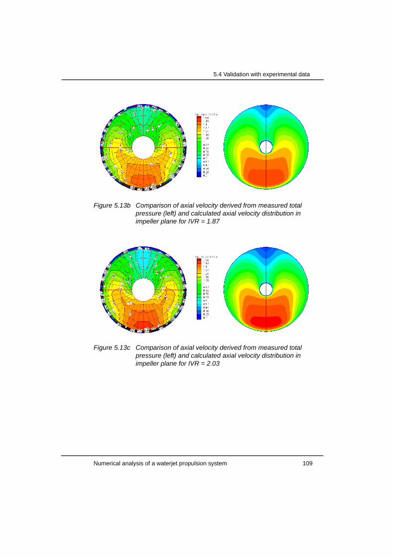
5.4 Validation with experimental data
Numerical analysis of a waterjet propulsion system 109
Figure 5.13b Comparison of axial velocity derived from measured total pressure (left) and calculated axial velocity distribution in impeller plane for IVR = 1.87
Figure 5.13c Comparison of axial velocity derived from measured total pressure (left) and calculated axial velocity distribution in impeller plane for IVR = 2.03

110
Chapter 5. Numerical analysis of waterjet inlet flow
Qualitative agreement between experimental data and calculated velocityfield is good for all four IVR conditions. The location and magnitude ofminimum and maximum axial velocity is predicted well with the numericalmethod.
The numerical results of the velocity distribution are compared to therepresentation of the measured data by Fourier-series (see section 3.1). Thedeviation between the two is used to quantify the relative error of thecalculated axial velocity. Figure 5.14 shows the relative difference for the bothlow IVR of 1.68 and the high IVR of 2.19.
The relative difference is defined as:
(5.6)
with vEXP based on the two dimensional Fourier representation of themeasured data.
The deviations are below 15% for a significant part of the cross-sectionalarea. It is concluded that the CFD analysis of the inlet flow reproduces thetypical non-uniform velocity distribution well. Therefore, the CFD methodemployed in the present investigation seems suitable for the investigation ofthe effect of non-uniform inflow into the mixed-flow waterjet pump.
Figure 5.13d Comparison of axial velocity derived from measured total pressure (left) and calculated axial velocity distribution in impeller plane for IVR = 2.19
∆vCFD vEXP–
vaver---------------------------------=

5.4 Validation with experimental data
Numerical analysis of a waterjet propulsion system 111
The velocity distributions show a clear increase of non-uniformity withincreasing IVR,i.e. decreasing vpump. The non-uniformity can be representedin a single value, if calculated according to equation (3.1). Figure 5.15 showsthe non-uniformity parameter ζ as a function of IVR. Both the results ofcalculations with wall and pressure boundary conditions have been used. Therelation between the IVR and the non-uniformity is shown clearly for the twotypes of boundary conditions. The small deviations are negligible.
Figure 5.14 Relative difference between experimental data and calculated axial velocity distribution at impeller plane for IVR = 1.68 (left) and IVR = 2.19
0
0.05
0.1
0.15
0.2
0.25
0.3
0.35
0.4
0.9 1.1 1.3 1.5 1.7 1.9 2.1 2.3
Wall boundaries
Pressure boundaries
Figure 5.15 Non-uniformity parameter ζ in impeller plane as function of IVR
IVR [-]
Non
-uni
form
ity ζ
[-]

112
Chapter 5. Numerical analysis of waterjet inlet flow
Figure 5.13d shows a region with very low axial velocity in the upper part ofthe cross-sectional area. For such conditions there may even be a region offlow recirculation upstream of the impeller plane.
The distribution of the magnitude of the velocity in the symmetry plane for twodifferent values of IVR, is shown in figure 5.16. At low IVR conditions theeffect of the bend on the velocity distribution can be recognised. At the innercorner of the inlet the velocity reaches a maximum value which reducesfurther downstream. This effect is less pronounced at high IVR conditions.
In the region in the bend above the shaft a very low velocity magnitude isobserved. Here flow separation is likely to occur at sufficiently high IVR, i.e.low values of vpump. The method to determine boundary layer separation willbe discussed in section 5.6, where additional flow phenomena in a waterjetinlet are reviewed.
Figure 5.16 Distribution of magnitude of velocity in symmetry plane for IVR 1.07 (top) and 2.03 (bottom)

5.4 Validation with experimental data
Numerical analysis of a waterjet propulsion system 113
5.4.5 Results obtained with k-ω turbulence model
The use of turbulence models in CFD calculations always provides reason fordiscussion. Though an in-depth study of effects of turbulence models on theflow in waterjets does not fit within the scope of this thesis, results ofcalculations with the k-ω turbulence model will be shown for comparison withresults of the k-ε turbulence model. The k-ω turbulence model is used widelyjust like the k-ε turbulence model. Often, the level of accuracy or the absenceof accuracy of a CFD calculation is attributed to the turbulence model used.Comparison of the experimental data with the results of calculationsemploying the k-ω turbulence model can show whether the result is sensitiveto the choice of a particular turbulence model.
Comparison of static pressure along ramp centre line
Figure 5.17 shows the static pressure distribution along the ramp ascalculated with the k-ω turbulence model. Agreement between calculationsand experimental data is good for all four presented conditions. Similarresults have been found for intermediate IVR conditions. The accuracy of thecalculations is comparable to the calculations with the k-ε turbulence model,as shown in figure 5.5. The main differences are in the region downstream ofthe shaft, where the pressure predicted by the method employing the k-ωmodel gives higher values than the ones predicted by the method using the k-ε model. This suggest that flow separation occurs later for the methodemploying the k-w model.
Figure 5.17 Comparison of measured and calculated static pressure along ramp centre line obtained with k-ω turbulence model
-0.3
-0.2
-0.1
0
0.1
0.2
0.3
0.4
0.5
0 200 400 600 800 1000 1200
ExperimentsCFD
IVR = 1.07IVR = 1.29IVR = 1.70IVR = 2.03
Distance along ramp [mm]
Cp
[-]

114
Chapter 5. Numerical analysis of waterjet inlet flow
Comparison of velocity field at impeller plane
The assessment of the performance of the k-ω turbulence model is not onlybased on the prediction of static pressure, but also on the prediction of thevelocity field. Figures 5.18a and b show the comparison of the velocitydistribution at the impeller plane for two IVR conditions. Agreement is goodfor both conditions.
The relative difference between calculations and data derived from themeasurements is shown in figure 5.19 for both conditions. The majority of thecross-sectional area has a difference below +/- 10%. Quantitative agreementseems to be slightly better with the k-ω turbulence model than with the k-εmodel, see figure 5.14.
Figure 5.18a Comparison of axial velocity derived from measurements (left) and calculated axial velocity distribution with k-ω turbulence model in impeller plane for IVR = 1.68
Figure 5.18b Comparison of axial velocity derived from measurements (left) and calculated axial velocity distribution with k-ω turbulence model in impeller plane for IVR= 2.19

5.4 Validation with experimental data
Numerical analysis of a waterjet propulsion system 115
5.4.6 Mesh convergence study
The mesh as used in this study has been made coarser and finer to evaluateto mesh convergence of the applied mesh. For the coarse mesh, the blockdivisions of the blocks near the symmetry plane of the original mesh arereduced by a factor of two in the direction perpendicular to the symmetryplane. In the direction along the cutwater the number of cells is reduced by afactor of two as well for the blocks near the cutwater. The reduction of cellsfrom the original mesh to the coarse mesh is about 30.000, but it should benoted that this reduction is achieved mainly in the region of the cutwater.
The fine mesh is derived from the original mesh by doubling all blockdivisions in all three directions. The number of cells in the normal direction of
the extrusion layer has been kept constant to remain at the same y+ values.
It should be noted, that the original medium mesh size has been developedabout 5 years ago. The number of cells of the original mesh, of about200.000, were governed by the hardware constrains of that time. Currently,the tools for generation of inlet meshes are used in the design procedure forwaterjet inlet geometries. In order to have calculation times, which areacceptable during the design phase, the default number of cells has not beenincreased. Nevertheless it is now possible to run the refined mesh, which hasabout 1.5 million cells.
The pressure distribution along the cutwater, as shown in figure 5.7 will bereviewed for the different meshes, because the largest gradient are present inthis region. Figure 5.20 shows the pressure coefficient for IVR = 1.87 alongthe cutwater for the three different meshes.
Figure 5.19 Relative difference between experimental data and calculated axial velocity distribution with k-ω turbulence model in impeller plane for IVR = 1.68 (left) and IVR = 2.19

116
Chapter 5. Numerical analysis of waterjet inlet flow
-1.2
-1
-0.8
-0.6
-0.4
-0.2
0
0.2
0.4
0.6
0.8
1
-10 -9 -8 -7 -6 -5 -4 -3 -2 -1 0
Coarse mesh (175.596 cells)
Medium mesh (206.884 cells)
Fine mesh (1.564.448 cells)
-1
-0.8
-0.6
-0.4
-0.2
0
0.2
0.4
0.6
0.8
1
1.2
-100 -80 -60 -40 -20 0 20 40 60 80 100
Coarse mesh (175.596 cells)
Medium mesh (206.884 cells)
Fine mesh (1.564.448 cells)
Distance s along cutwater [mm]
Cp
[-]
s<0
s>0
s=0
Figure 5.20 Calculated pressure coefficient Cp along the cutwater for different mesh sizes for IVR of 1.87. Top figure shows s range of -100 to 100 and bottom figure shows region with location of minimum pressure, located between s range of -10 and 0. Negative s coordinate represents lower side of cutwater and positive coordinate represents upper side.
Distance s along cutwater [mm]
Cp
[-]
s<0
s>0
s=0

5.5 Analysis of the suction streamtube
Numerical analysis of a waterjet propulsion system 117
The region with the location of the minimum pressure is shown in detail in thesecond diagram. The markers in this figure represent the corner points of thecells.
Increase of the number of cells with a factor of 8 results in a difference of theprediction of minimum pressure ∆cp=0.06 for this condition. The difference isfound along a small part of the cutwater region of about 2 mm, which is 1.3%of the inlet diameter.
The difference in pressure distribution along the cutwater between theoriginal mesh and the fine mesh is regarded to be representative for thecomplete mesh. Since the deviations between the two meshes are limited toa small region near the cutwater and the magnitude of the difference is small,is it concluded that the cell sizes of the original mesh are suitable for thepresented study.
5.4.7 Closing remarks
Agreement between the experimental data and the results of the calculationsis quite good, despite the mentioned deficits of the k-ε turbulence model.Performance of the k-ω turbulence is comparable. It is not an aim tobenchmark turbulence models in this study, and therefore the k-ε model isused in the remainder of the analyses.
One aspect of the use of RANS methods has not been addressed yet. This isthe capability to calculate the flow for geometries according to full scaledimensions with full scale boundary conditions. Calculations of full scalewaterjet inlets only require a refinement of the cells near the solid walls in
order to keep acceptable y+ values. The thickness of the actual hull boundarylayer can be applied at the inflow boundary condition. In this way, the effect ofa thicker boundary layer, due to an increase in the length of a vessel, can betaken into account for example.
5.5 Analysis of the suction streamtube
The preceding section covers the comparison of measured and calculatedresults. Typical quantities which can be measured in experimental facilitiesare total and static pressure. Velocities can be derived from this dataafterwards. The CFD results provide a wide range of additional post-processing capabilities to get more insight into the behaviour of the flow.Examples include the calculation of shear stresses along the inlet surfaceand the determination of the suction streamtube. The CFD results used in thissection are the results obtained for the waterjet inlet without tunnel walls, thisin order to avoid possible effects of the confinement on the flow of thepresence of the cavitation tunnel walls.

118
Chapter 5. Numerical analysis of waterjet inlet flow
5.5.1 Visualisation of suction streamtube
The CFD method provides a way to introduce a concentration scalar as apassive traces in the flow field. This concentration scalar can be implementedat inlet or pressure boundaries and it can be used as a weight function forfurther analysis.
The shape of the streamtube is not known in advance. In fact, only at theimpeller plane the streamtube is known to coincide with the impeller planeboundary. Setting the concentration factor to 100% in the impeller planeallows for the determination of the complete streamtube with a upstreamtracing method. In this approach the flow field is reversed and frozen, which isallowed in a steady flow problem. With the frozen velocity field, the solution ofthe scalar only takes a few iterations for the complete numerical domain.
The shape of the streamtube is derived from an iso-surface plot of theconcentration. In this way a clear representation of the streamtube interfacecan be obtained. An example of the three-dimensional streamtubevisualisation is shown in figure 5.21 from different view angles.
5.5.2 Determination of suction streamtube shape
The shape of the suction streamtube at the inlet boundary of the domain canbe used to calculate the average ingested velocity vin. This velocity is used inthe calculation of the wake fraction w and the thrust of the installation.Determination of the cross-sectional area of the streamtube at severallocations upstream of the impeller plane provides information about thediffusor effect in the streamtube. The values of the cross-sectional areas canbe used to calculate the equivalent diffusor angles. This will give an indicationof the risk of the onset of boundary layer separation in the inlet duct.
Figure 5.21 Visualisation of three-dimensional suction streamtube for IVR=1.29

5.5 Analysis of the suction streamtube
Numerical analysis of a waterjet propulsion system 119
Cross-sectional shape of streamtube at inlet boundaryThe shape of the suction streamtube at the inlet boundary of the numericaldomain can be approximated with a semi-elliptical shape. An example isgiven in figure 5.22 for a range of IVR values. The boundary of thestreamtube can be approximated by the ellipse:
(5.7)
where 2w0 and h0 are the maximum width and maximum height resp. These
two parameters are determined by employing a least-square fit of the datadetermined from the computed streamtube surface cross-section at the inletplane of the computational domain.
The elliptical curve fit can be used to determine the mass averaged inflowvelocity of the ingested fluid out of the boundary layer. In the calculations apower-law exponent n=7 and a boundary layer thickness of 0.3D, with D theinlet diameter, is used.
An efficient method to determine the inflow velocity is based on theintegration of the streamtube velocity. Once the concentration scalar is
yw0------ 2 z
h0----- 2
+ 1=
Figure 5.22 Computed semi-elliptical shape of suction streamtube at inlet of numerical domain for various IVR conditions
-0.6
-0.5
-0.4
-0.3
-0.2
-0.1
0
0.0 0.2 0.4 0.6 0.8 1.0 1.2
IVR 1.07
IVR 1.29
IVR 1.70
IVR 2.03
IVR 1.07 - elliptic fit
IVR 1.29 - elliptic fit
IVR 1.70 - elliptic fit
IVR 2.03 - elliptic fit
y/D [-]
z/D
[-]

120
Chapter 5. Numerical analysis of waterjet inlet flow
available, the mass averaged inflow velocity can be determined by simpleintegration:
(5.8)
In this equation the concentration scalar is denoted by c and x is the directionnormal to the inflow area Ainflow.
Figure 5.23 shows the calculated wake fraction w (as defined in equation(2.2)) based on the elliptical streamtube shape and on direct integration of theCFD results. The rectangular box approach is also plotted for three differentwidths of the box.
The method of direct integration and the method of the elliptical curve fit givemore or less comparable results for the wake prediction. The method, basedon a rectangular streamtube with a width of 1.3D, gives an underestimation ofthe wake fraction of about 20%. The other two curves for the rectangular box,based on 1.6D and 1.9D, show that a width depending on IVR is required toobtain a good fit. It is acknowledged that the value of 1.3D is an empiricalfactor, which has been derived in the past to obtain good correlations with theactual sailing fleet.
vin
ρ c vx2⋅( ) Ad
Ainflow
∫
ρ c vx⋅( ) Ad
Ainflow
∫------------------------------------------=
Figure 5.23 Calculated wake fraction w based on elliptical fit, rectangular box method and direct integration of CFD results.
0
0.02
0.04
0.06
0.08
0.1
0.12
0.14
0.16
0.9 1.1 1.3 1.5 1.7 1.9 2.1 2.3
Ellips curve fit
Direct integration
Rectangular box - 1.3 D
Rectangular box - 1.6 D
Rectangular box - 1.9 D
IVR [-]
Wak
e fr
actio
n w
[-]

5.5 Analysis of the suction streamtube
Numerical analysis of a waterjet propulsion system 121
Cross-sectional area of streamtube
In the preceding section the cross-sectional shape of the streamtube at theinflow boundary has been discussed. Here the development of the cross-sectional area of the streamtube will be analysed in more detail. The cross-sectional area has been determined at 9 different stations. The cross-sections are taken perpendicular to the ramp surface from the inlet boundaryto the cutwater, as shown in figure 5.24. The area is determined byintegration of the concentration factor over the whole plane:
(5.9)
where n is the integration plane index number, in the range 1 to 9.
Figure 5.25 shows the development of the cross-sectional area of thestreamtube. The areas are normalised with the streamtube area at plane 9.This area is denoted as intake throat area [2]. The distances are calculatedfrom the first plane to the throat area.
Atube c Ad
An
∫=
Figure 5.24 Location of streamtube cross-sections. The parameter s is the length along the waterjet inlet contour in the plane of symmetry.

122
Chapter 5. Numerical analysis of waterjet inlet flow
Far upstream, near the inflow plane, a constant cross-sectional area is foundfor each IVR condition. The influence of the ramp curvature, at cross-sectionnumbers 4 and 5, can be recognised as a small region of reduced area,which is due to an acceleration of the flow. The typical retardation of the flowat higher IVR (i.e. lower vpump) conditions is reflected in a steep increase ofthe streamtube area when approaching the inlet lip.
The development of the streamtube in streamwise direction can also beexpressed in an equivalent diffuser angle αdiff. This diffusor angle is based onthe equivalent streamtube diameter and the distance dl between the differentcross-sections:
(5.10)
The equivalent diameter is based on a circular section with area identical tothe area of the streamtube cross-section. The variation of the equivalentdiameter along the streamtube in streamwise direction has been fitted with afifth order polynomial. With this curve fit the diffuser angle αdiff can be derivedin small steps of the length dl.
The development of the diffusor angle along the streamtube up to thecutwater is shown in figure 5.26 for various IVR values.
Figure 5.25 Streamtube cross-sectional area normalised by A9. The numbers refer to the integration plane index numbers, as shown in figure 5.24.
0
0.2
0.4
0.6
0.8
1
1.2
0 1 2 3 4 5 6 7 8
IVR = 1.07
IVR = 1.21
IVR = 1.29
IVR = 1.50
IVR = 1.70
IVR = 1.87
IVR = 2.03
IVR = 2.19
Dimensionless distance s/D [-]
Nor
mal
ised
are
a A
/A9[
-]
2 3 4 5 6 7 8 9
αdiff
Dn 1+ Dn–
dl--------------------------- atan=

5.6 Evaluation of wall shear stress
Numerical analysis of a waterjet propulsion system 123
At the ramp curvature (around s/D = 3.5), all conditions show a smallnegative value of αdiff, which represents the contraction of the streamtube. AtIVR conditions of 1.87 and higher, the diffuser angle exceeds 8 degrees. Atsuch high diffuser angles, flow separation is likely to occur in normal circulardiffusers [15]. The occurrence of flow separation will be discussed in moredetail in the following subsection.
5.6 Evaluation of wall shear stress
Evaluation of the wall shear stress in the inlet duct can provide informationabout the probability of flow separation in the inlet. Flow separation will leadto increased non-uniformity of the flow in the impeller plane and higherhydraulic losses. This is a deterioration of the performance of the wholepropulsion system and should be avoided in the range of normal operatingconditions. Boundary layer separation will occur inside the inlet duct at theramp side, because of the strong adverse pressure gradient acting on theflow. Occurrence of this large pressure gradient at high IVR (i.e. low vpump)has already been demonstrated in figure 5.5 in subsection 5.4.1.
Determination of a possible region of separated flow is based on themagnitude of the wall shear stress along the duct. It is assumed that theonset of separation occurs at the location where the wall shear stress
Figure 5.26 Equivalent diffuser angle αdiff of streamtube
-4
-2
0
2
4
6
8
10
12
0 1 2 3 4 5 6 7 8
IVR = 1.07
IVR = 1.21
IVR = 1.29
IVR = 1.50
IVR = 1.70
IVR = 1.87
IVR = 2.03
IVR = 2.19
Dimensionless distance s/D [-]
α diff
[deg
rees
]

124
Chapter 5. Numerical analysis of waterjet inlet flow
reduces to a zero value [16]. The dimensionless wall shear stress is denotedas the dimensionless friction velocity vf:
(5.11)
The non-dimensional representation can be used to get a morecomprehensive comparison of calculations for varying pump velocity.
For the standard flush-type inlet geometries, possible flow separation islocated inside the duct near station 9 (as shown in figure 5.24). The wallshear stress component in axial direction will change sign in case ofboundary layer separation in this region. For the detection of flow separation,the friction velocity is multiplied with the sign of the axial wall shear stress.
Figure 5.27 shows the result of the evaluation of the minimum wall shearstress at the waterjet inlet duct part. Results of calculations with both wall aswell as pressure boundaries are used in this evaluation. The differencebetween the results of both series of calculations is negligible.
According to the wall shear stress criterion, flow separation will occur for IVRvalues higher than 1.75. This is in accordance with the maximum allowablediffuser angle criterion of 8 degrees (as shown in figure 5.26).
For a practical inlet design, flow separation should not occur at normaloperating conditions. With a dedicated inlet geometry design it is possible toavoid flow separation in the inlet for all operating conditions.
vfτw
ρvpump2
--------------------=
-0.03
-0.02
-0.01
0
0.01
0.02
0.03
0.9 1.1 1.3 1.5 1.7 1.9 2.1 2.3
Wall boundaries
Pressure boundaries
Figure 5.27 Dimensionless wall shear stress as function of IVR
IVR [-]
Fric
tion
velo
city
vf [
-]

5.7 Nomenclature
Numerical analysis of a waterjet propulsion system 125
5.7 Nomenclature
A area m2
c concentration -
Cp pressure coefficient -
g gravitational acceleration m/s2
h height from tunnel centre line to cutwater m
h0 maximum suction depth m
IVR inlet velocity ratio (vship/vpump) -
p static pressure N/m2
p0 static ambient pressure in tunnel N/m2
pv vapour pressure N/m2
v velocity m/s
vf friction velocity -
w0 maximum suction half width m
y,z coordinates m
Greek symbols
ρ fluid density kg/m3
σ cavitation inception pressure -
τw wall shear stress N/m2
Subscripts
n normal direction
pump based on values just upstream of the impeller
tunnel based on tunnel values
x axial direction
5.8 References
[1] Førde, M., Ørbekk, E., Kubberud, N., ‘Computational Fluid Dynamicsapplied to high speed craft with special attention to water intake forwater jets’, FAST’91 conference, pp. 69-89, Trondheim, 1991
[2] Terwisga, T.J.C. van,’Waterjet-hull interaction’, PhD thesis, TechnicalUniversity of Delft, 1996
[3] Pylkkänen, J.V.,’Test cases of application of CFD code to predictwaterjet inlet flows’, Technical report VTT VAL B-11, VTT Manufactur-ing Technology, Maritime Research, Espoo, 1994

126
Chapter 5. Numerical analysis of waterjet inlet flow
[4] Pylkkänen, J.V.,’CFD analysis and iterative design of waterjet inlet’,International conference on ship and marine research, Rome, 1994
[5] Vorst, H.J.A. van der, Verbeek, R., Hendriks, A.J.A.M., ‘Design consid-erations of waterjet propulsion systems’, 13th Fast Ferry InternationalConference, Singapore, 1997
[6] Seil, G.J., Fletcher, C.A.J., Doctors, L.J., ‘The application of computa-tional fluid dynamics to practical waterjet propulsion system design andanalysis’, Proceedings of the 3rd international conference on Fast SeaTransportation, pp 1379-1390, Lubeck-Travemunde, 1995
[7] Yang, C.K., Lee, Y.B., Choi, H.S., ‘A numerical analysis of the flowaround the waterjet inlet’, Proceedings of the 3rd international confer-ence on Fast Sea Transportation, pp 1391-1401, Lubeck-Travemunde,1995
[8] Bulten, N.W.H.,‘Influence of boundary layer ingestion on waterjet per-formance parameters at high ship speeds’, Proceedings of the 5thinternational conference on Fast Sea Transportation, pp 883-892,Seattle, 1999
[9] Hu, P., Zangeneh, M., ‘Investigations of 3D turbulent flow inside andaround a water-jet intake duct under different operating conditions’,ASME Journal of Fluids Engineering, Vol 121, pp. 396-404, 1999
[10] Hu, P., Zangeneh, M., ‘A method for automatic optimisation of theintake duct geometry of marine water-jets’, Proceedings of the 5thinternational conference on Fast Sea Transportation, pp 843-851,Seattle, 1999
[11] Brandner P., Walker, G.J.,’A waterjet test loop for the Tom Fink cavita-tion tunnel’, Proceedings Waterjet Propulsion III conference, Gothen-burg, 2001
[12] Versteeg, H.K., Malalasekera, W., ‘An introduction to ComputationalFluid Dynamics’, Longman Scientific & Technical, Essex, 1995
[13] Computational Dynamics Limited, ‘Star-CD methodology, version3.150’, 2001
[14] Patankar, S.V., Spalding, D.B., ‘A calculation procedure for heat, massand momentum transfer in three-dimensional parabolic flows’, Int. J.Heat Mass Transfer, Vol 15, pp. 1787-1806
[15] Schlichting, H., ‘Boundary layer theory’, McGraw-Hill, New York, 1968.
[16] Fox, R.W., McDonald, A.T., ’Introduction to fluid mechanics’, Third edi-tion, John Wiley & Sons, New York, 1985

Numerical analysis of a waterjet propulsion system 127
Chapter 6 Numerical analysis of waterjet pump flow
This chapter deals with the numerical analysis of the mixed-flow waterjetpump. The geometry and mesh generation procedure will be discussed insection 6.1. The numerical domain encloses the impeller, the stator bowl anda straight suction pipe. Subsequently, in section 6.2, the choice of boundaryconditions and the options for implementation of impeller rotation arereviewed. In section 6.3, results of the CFD calculations with uniform infloware compared with available experimental data to get an indication of theaccuracy of the numerical method used. The experimental data is measuredduring the development of the waterjet pump and is only available at theauthors’ company. This data is used for the prediction of the performance ofthe full scale installations.
The influence of a non-uniform inflow on the performance is presented insection 6.4. Its effect on the radial loading of the impeller is treated as well.The axial velocity distributions as shown in the previous chapters, are usedas input velocity distributions.
6.1 Geometry and mesh generation
The numerical domain for the analysis of the flow through the mixed-flowpump includes the complete impeller and the stator bowl with guide vanes.Preliminary calculations assuming periodic flow, i.e. reducing the calculationto computing the flow through a single impeller channel showed pooragreement with experimental data. This can be partly attributed to the appliedboundary condition of constant pressure at the outlet part of the numerical
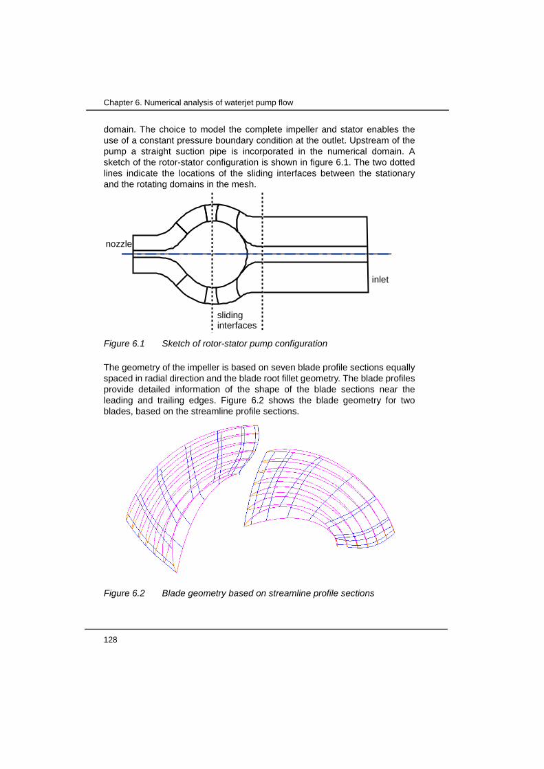
128
Chapter 6. Numerical analysis of waterjet pump flow
domain. The choice to model the complete impeller and stator enables theuse of a constant pressure boundary condition at the outlet. Upstream of thepump a straight suction pipe is incorporated in the numerical domain. Asketch of the rotor-stator configuration is shown in figure 6.1. The two dottedlines indicate the locations of the sliding interfaces between the stationaryand the rotating domains in the mesh.
The geometry of the impeller is based on seven blade profile sections equallyspaced in radial direction and the blade root fillet geometry. The blade profilesprovide detailed information of the shape of the blade sections near theleading and trailing edges. Figure 6.2 shows the blade geometry for twoblades, based on the streamline profile sections.
Figure 6.1 Sketch of rotor-stator pump configuration
inlet
nozzle
sliding interfaces
Figure 6.2 Blade geometry based on streamline profile sections

6.1 Geometry and mesh generation
Numerical analysis of a waterjet propulsion system 129
Around the cross-sections of the blades, an O-grid is used to ensure goodorthogonality of the boundary layer cells along the impeller surface. Thesecells are also used in the region near the hub surface. The remainder of thevolume between the impeller blades is filled with additional hexagonal cells.
The stator bowl is meshed with another group of hexagonal cells, whichfollow the guide vanes curvature. Thickness of the guide vanes is taken intoaccount in the model. The shaft is included in the model at the suction side ofthe impeller, like in a real waterjet installation.
Figure 6.3 shows the topology of the mesh between two impeller blades in aplane at half-span and the block topology from hub to tip.
At the seatring, very fine cells are created from an extrusion layer. In thisregion high gradients occur due to the seatring being stationary with respectto the rotating unschrouded impeller. The layer of extruded cells fills the tipregion between the impeller blades and the seatring. In this way, water canflow over the tip from pressure to the suction side of the blade. Treatment ofthe tip clearance is in agreement with the findings of several studies of turbomachinery addressing tip clearance flow phenomena [1-4].
Figure 6.3 Mesh topology for the impeller of the mixed-flow pump in a plane at half-span (top) and in the direction from hub to tip

130
Chapter 6. Numerical analysis of waterjet pump flow
Figure 6.4 shows the surface plot of the impeller blades, the stator blades, thehub and the shaft. The final mesh of the complete mixed-flow pump ispresented in figure 6.5. The total number of cells is about 950.000 for thecomplete mesh.
Figure 6.4 Surface plot of impeller blades, stator blades, hub and shaft
inletnozzle
Figure 6.5 Complete mesh of the mixed-flow pump with about 950.000 cells (top) and surface mesh of the impeller
inlet
rotorstator
nozzle
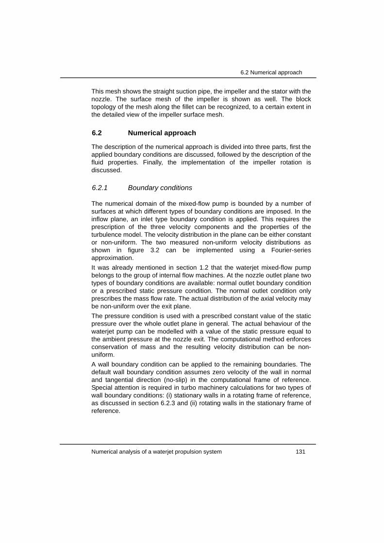
6.2 Numerical approach
Numerical analysis of a waterjet propulsion system 131
This mesh shows the straight suction pipe, the impeller and the stator with thenozzle. The surface mesh of the impeller is shown as well. The blocktopology of the mesh along the fillet can be recognized, to a certain extent inthe detailed view of the impeller surface mesh.
6.2 Numerical approach
The description of the numerical approach is divided into three parts, first theapplied boundary conditions are discussed, followed by the description of thefluid properties. Finally, the implementation of the impeller rotation isdiscussed.
6.2.1 Boundary conditions
The numerical domain of the mixed-flow pump is bounded by a number ofsurfaces at which different types of boundary conditions are imposed. In theinflow plane, an inlet type boundary condition is applied. This requires theprescription of the three velocity components and the properties of theturbulence model. The velocity distribution in the plane can be either constantor non-uniform. The two measured non-uniform velocity distributions asshown in figure 3.2 can be implemented using a Fourier-seriesapproximation.
It was already mentioned in section 1.2 that the waterjet mixed-flow pumpbelongs to the group of internal flow machines. At the nozzle outlet plane twotypes of boundary conditions are available: normal outlet boundary conditionor a prescribed static pressure condition. The normal outlet condition onlyprescribes the mass flow rate. The actual distribution of the axial velocity maybe non-uniform over the exit plane.
The pressure condition is used with a prescribed constant value of the staticpressure over the whole outlet plane in general. The actual behaviour of thewaterjet pump can be modelled with a value of the static pressure equal tothe ambient pressure at the nozzle exit. The computational method enforcesconservation of mass and the resulting velocity distribution can be non-uniform.
A wall boundary condition can be applied to the remaining boundaries. Thedefault wall boundary condition assumes zero velocity of the wall in normaland tangential direction (no-slip) in the computational frame of reference.Special attention is required in turbo machinery calculations for two types ofwall boundary conditions: (i) stationary walls in a rotating frame of reference,as discussed in section 6.2.3 and (ii) rotating walls in the stationary frame ofreference.

132
Chapter 6. Numerical analysis of waterjet pump flow
6.2.2 Fluid properties
The fluid properties are specified similar to the ones specified for thecalculations of the flow through the waterjet inlet as discussed in section5.3.2. The density and viscosity are taken constant for the fluid. Turbulence ismodelled with the k-ε turbulence model.
6.2.3 Impeller rotation
The basic idea is to split the numerical domain into three different parts:stationary inlet part, a rotating impeller part and a stationary stator bowl part.Rotation of the impeller can be accounted for in two different ways: (i) aquasi-steady approach with a multiple-frames-of-reference (MFR) method, or(ii) a fully transient method with a mesh moving with the impeller and withsliding interfaces with the stationary part of the mesh.
The MFR method is a relatively fast method, which can be used with asteady-flow solution method. This method is identical to the method used forthe waterjet inlet flow calculations. In a rotating frame of reference rotation ofthe impeller results in centrifugal and Coriolis forces on the fluid elements.These are implemented by additional source terms in the momentumequations.
In case of a moving mesh with a sliding interface, a fully transient flowsolution method is required. The CFD method provides a routine, whichautomatically rotates the mesh after each timestep and connects the rotatingand stationary domains. Fully transient flow calculations use the PISO(Pressure Implicit with Splitting of Operators) algorithm to couple themomentum and pressure terms. This algorithm was originally developed forthe non-iterative computation of unsteady compressible flow [5]. It involvesone predictor step and two or more corrector steps, which may be seen as anextension of the SIMPLE algorithm with additional corrector steps.
All calculations presented in this chapter have been made for an impellerrotational speed of 1920 RPM, (32 Hz). Reynolds numbers based on inletpump diameter and rotational speed (according to equation (4.1)) are in
excess of . Note that full scale waterjet installations normally operate atReynolds numbers which are 3 to 5 times larger.
6.2.4 Calculation of global pump performance
Pump head
By definition, pump head is based on the difference in total pressureupstream and downstream of the pump (see (2.32)). These values can bederived from the CFD results by integration of the total pressure over a cross-
107

6.2 Numerical approach
Numerical analysis of a waterjet propulsion system 133
sectional area upstream and downstream of the impeller. It follows from theenergy balance, that mass averaged quantities are to be used to determinethe total pressure:
(6.1)
where A denoting the cross-sectional plane. The actual mass averaged headHma is calculated as:
(6.2)
In an experimental set-up it is common practice to divide the total pressureinto a static and a dynamic pressure component. Static pressure is measuredat the inlet and outlet pipe circumference through pressure taps. Estimation ofthe dynamic pressure contribution is based on the inlet and outlet pipediameter and the volume flow through the pump. Within this approach it isassumed that the velocity and pressure distributions are uniform over themeasurement planes, and that there are no significant velocity components inthe tangential and radial direction (i.e. swirl).
The calculation of the head from the CFD calculations can also be based onthe static pressure distribution and the flow rate. The area-averaged staticpressure is calculated according to:
(6.3)
where A represents the cross-sectional area. It is acknowledged, that inactual experiments, the static pressure is only measured at the outer radiusand subsequently averaged. This difference is neglected in the analysis. Thearea-averaged head becomes:
(6.4)
There are therefore two expressions for the head of the pump: the correctvalue Hma, based on a mass average, and an estimated value Haa, based onarea averages. The non-uniformity of the axial inflow velocity is taken intoaccount with the mass averaged method correctly, but not with the areaaveraged method.
ptot1
ρQ-------- ρptotvn Ad
A∫=
Hma
ptot o, ut ptot in,–
ρg---------------------------------------=
pstat1A---- pstat Ad
A∫=
Haa
pstat out, pstat in,–
ρg--------------------------------------------- Q
2
2g------- 1
Aout2
----------- 1
Ain2
--------–
+=

134
Chapter 6. Numerical analysis of waterjet pump flow
Shaft torque
In an experimental set-up, shaft torque can be measured with strain gaugeson the shaft. The measured torque can be corrected for additional frictionlosses in seals and bearings. In the CFD calculations torque can bedetermined in two ways. The first method is based on a direct summation ofwall forces acting on the impeller and shaft surface. The second method isbased on a momentum balance in circumferential direction. The equation forthe moment of momentum is given by (see for example [6]):
(6.5)
where CV represents the control volume and CS all surfaces of the controlvolume, r is the distance from the axis of rotation, v is the velocity and τw theviscous stress tensor. In general turbo machinery applications, the axialcomponent of this vector equation has to be evaluated only. For steady flowconditions the equation for moment of momentum reduces to:
(6.6)
where vt is the circumferential velocity component, vn the normal velocity atcontrol surfaces and τw,t the tangential shear force at the surfaces of thestationary housing. This force will be a result of the shear forces acting on thesurface of the so-called seatring. Evaluation of the first term on the right handside of equation (6.6) can be limited to the surfaces through which the flowenters and leaves the control volume, since the normal velocity vanishes atwall surfaces. The actual equation for the determination of the torque withinthe numerical method becomes:
(6.7)
6.3 Validation with experimental data
The numerical method used to compute the flow in the waterjet mixed-flowpump is validated with the aid of experimental data of pump performance.Extensive series of measurements have been made on a model-scale pumpat the authors’ company. The experimental data include the head and torquecurves as a function of flow rate. The pump performance data is used in thewaterjet performance prediction software of Wärtsilä Propulsion Netherlands
Tshaft t∂∂ r v×
CV∫ ρdV r vρv× Ad⋅
CS∫ r τw×
CS∫–+=
Tshaft ρrvtvn Ad
CS∫ rτw t,
CS∫–=
Tshaft ρrvtvn Ad
Aout
∫ ρrvtvn Ad
Ain
∫ rτw t,Aseatring
∫––=

6.3 Validation with experimental data
Numerical analysis of a waterjet propulsion system 135
BV. The performance prediction software has been used for the prediction ofall full scale installations, which are currently in service.
Flow rate and head are expressed as non-dimensional quantities withequations (2.15) and (2.16) respectively. Torque is presented as a non-dimensional quantity as well. This is similar to the torque coefficient Kq usedfor propellers. The non-dimensional torque is defined as:
(6.8)
Pump efficiency is derived from the values for the flow rate, head and torque,based on equation (2.20).
6.3.1 Quasi-steady flow calculations with the MFR method
Results of CFD calculations with the method using the quasi-steady multipleframe of reference approach are presented in this section.
Head curve
First the head curve based on the CFD calculations will be compared with theexperimental data. Figure 6.6 shows the dimensionless head curves from themeasurements and the calculations. The calculated head is based onequations (6.2) and (6.4). The presented head curves are normalised with aconstant given flow rate and pump head of the design condition. Agreementbetween the calculations and the experimental data is good over a largerange of flow coefficients.
Differences between the two methods to determine the head from the CFDresults are limited to the low flowrate conditions. Near the design point thedeviations between the two approaches are negligible. The differencesbetween the two methods at low flow rates can be attributed to a non-uniformvelocity distribution at the outlet.
The numerical results are used to express the differences between massaveraged and area averaged determination of the head. These calculationsare based on a pump configuration with a nozzle, which has ambientpressure at the exit area. The measurements are made in a closed-loopsystem however. The measured head will give the correct value,corresponding with the mass averaged numerical prediction, when the staticmeasurement locations are located sufficiently far upstream and downstreamof the pump to ensure uniform velocity distributions at those locations.
T* T
ρΩ2D
5------------------=

136
Chapter 6. Numerical analysis of waterjet pump flow
Gülich et al [7] show the obtained accuracy of calculated pump head for alarge number of different pumps with a RANS method. Comparisons withmeasured data show deviations up to about 4% for mixed-flow type pumps.Deviations of 5% in head prediction are also presented for a complete stageof a boiler feed pump [8]. The currently found deviations betweenmeasurements and calculations are of the same order or smaller. It can beconcluded that the prediction of head with the CFD method is sufficientlyaccurate for further analysis of the complete waterjet installation in chapter 7.
Shaft torque
A comparison of the calculated and measured shaft torque is shown in figure6.7. Calculation of torque is based on the integration of the wall forces and onthe moment of momentum balance (equation (6.7)). Differences between theresults of the two numerical methods are negligible for all conditions.Agreement between the numerical results and the measured data isacceptable over the whole range of analysed conditions.
The magnitude of the differences appears to be related to the flow rate,where an under-estimation is observed at low flow rates and an over-estimation at high flow rates. The differences are limited to a few percent atmost, however, in the range considered.
Figure 6.6 Comparison of measured and calculated head curves, based on equations (6.2) and (6.4).
0%
20%
40%
60%
80%
100%
120%
140%
160%
180%
200%
50% 60% 70% 80% 90% 100% 110% 120%
CFD_H_mass-averaged
CFD - H_area-averaged
Measurements
Q/Qbep [%]
H/H
bep
[%]

6.3 Validation with experimental data
Numerical analysis of a waterjet propulsion system 137
Efficiency
The efficiency of a pump has been defined in equation (2.20) as the ratio ofthe hydraulic power and the shaft power. Hydraulic power is the product ofvolume flow rate and the produced pressure head. Shaft power is the productof torque and the impeller angular speed. Based on the graphs of head andtorque, it is to be expected that the calculated pump efficiency will show somedeviations compared to the experimental data.
Figure 6.8 shows the calculated and the measured normalised efficiency ofthe pump. The calculated efficiency is based on the head according toequation (6.2), and the torque based on integration of the wall forces. Thepump efficiency is normalised with the efficiency at the design point.
The deviation between the calculated and the measured efficiency is about1% near the design flow rate.
Figure 6.7 Comparison of measured and calculated shaft torque based on integration of wall forces and moment of momentum balance
50%
60%
70%
80%
90%
100%
110%
120%
130%
140%
150%
50% 60% 70% 80% 90% 100% 110% 120%
CFD_wall force integration
CFD_moment of momentum balance
Measurements
Q/Qbep [%]
T*/
T* b
ep [%
]
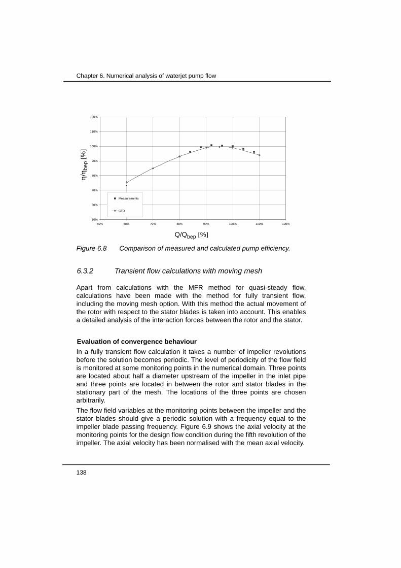
138
Chapter 6. Numerical analysis of waterjet pump flow
6.3.2 Transient flow calculations with moving mesh
Apart from calculations with the MFR method for quasi-steady flow,calculations have been made with the method for fully transient flow,including the moving mesh option. With this method the actual movement ofthe rotor with respect to the stator blades is taken into account. This enablesa detailed analysis of the interaction forces between the rotor and the stator.
Evaluation of convergence behaviour
In a fully transient flow calculation it takes a number of impeller revolutionsbefore the solution becomes periodic. The level of periodicity of the flow fieldis monitored at some monitoring points in the numerical domain. Three pointsare located about half a diameter upstream of the impeller in the inlet pipeand three points are located in between the rotor and stator blades in thestationary part of the mesh. The locations of the three points are chosenarbitrarily.
The flow field variables at the monitoring points between the impeller and thestator blades should give a periodic solution with a frequency equal to theimpeller blade passing frequency. Figure 6.9 shows the axial velocity at themonitoring points for the design flow condition during the fifth revolution of theimpeller. The axial velocity has been normalised with the mean axial velocity.
Figure 6.8 Comparison of measured and calculated pump efficiency.
50%
60%
70%
80%
90%
100%
110%
120%
50% 60% 70% 80% 90% 100% 110% 120%
Measurements
CFD
Q/Qbep [%]
η/η b
ep [%
]

6.3 Validation with experimental data
Numerical analysis of a waterjet propulsion system 139
For the monitoring points upstream of the impeller constant values can beobserved, due to the prescribed axial inflow velocity. Downstream of theimpeller a periodic solution is found for all three monitoring points. Theaverage value and the amplitude depend on the location of the monitoringpoints. The signal shows that during the fifth revolution of the impeller thesignal is periodic with frequency equal to the blade passing frequency (BPF).
The fluctuating pressure coefficients at the monitoring points is shown infigure 6.10. The pressure coefficient is defined as:
(6.9)
where p0 is the reference pressure at the nozzle exit plane, ρ the density, Ωthe shaft speed and D the diameter of the inlet.
The monitoring points downstream of the impeller show the expected periodicbehaviour of the pressure. The monitoring points upstream of the impellershow fluctuations also containing higher frequencies. Pressure fluctuations atthe inlet side are related to the choice of the boundary conditions at both theinlet and outlet boundary. The constant pressure boundary condition impliesthe pressure being steady at the nozzle exit surface. As a consequence, anyfluctuation in the overall pressure head is experienced at the inlet. On the
Figure 6.9 Normalised axial velocity at monitoring points during fifth impeller revolution for design condition. Points 1,2 and 3 are located upstream of the impeller, points 4,5 and 6 are located in between the impeller and stator.
0.8
0.9
1
1.1
1.2
1.3
1.4
4.00 4.10 4.20 4.30 4.40 4.50 4.60 4.70 4.80 4.90 5.00
Point 1
Point 2
Point 3
Point 4
Point 5
Point 6
Number of revolutions [-]
Nor
mal
ised
axi
al v
eloc
ity[-
]
3
2
1
6
4
5
Cp
pstat p0–
12---ρΩ2
D2
------------------------=

140
Chapter 6. Numerical analysis of waterjet pump flow
other hand, in an actual pump, small fluctuations in mass flow will be present,which may limit the high frequency pressure fluctuations. In the calculationsthe mass flow rate is a constant prescribed value due to the prescription of afixed velocity at the inlet side.
Evaluation of the periodic behaviour of the solution is based on a Fourier-transformation of the fluctuations. Figures 6.11 and 6.12 show the Fouriertransforms for both the axial velocity and the pressure at the design flow ratecondition for the monitoring points, which are located downstream of theimpeller, i.e. in between the impeller and the stator.
The peaks at the impeller-blade passing frequency and its higher harmonicscan be recognised easily. The Fourier transformations show a clear harmonicsolution downstream of the impeller for both the axial velocity as well as thestatic pressure. Results of the Fourier analyses for other flow rates arepresented in Appendix B.
Figure 6.10 Static pressure coefficient at monitoring points during fifth impeller revolution for design condition. Points 1,2 and 3 are located upstream of the impeller, points 4,5 and 6 are located in between the impeller and stator.
0
0.05
0.1
0.15
0.2
0.25
4.00 4.10 4.20 4.30 4.40 4.50 4.60 4.70 4.80 4.90 5.00
Point 1
Point 2
Point 3
Point 4
Point 5
Point 6
Number of revolutions [-]
Pre
ssur
e co
effic
ient
Cp
[-]
3
2
1
6
4
5
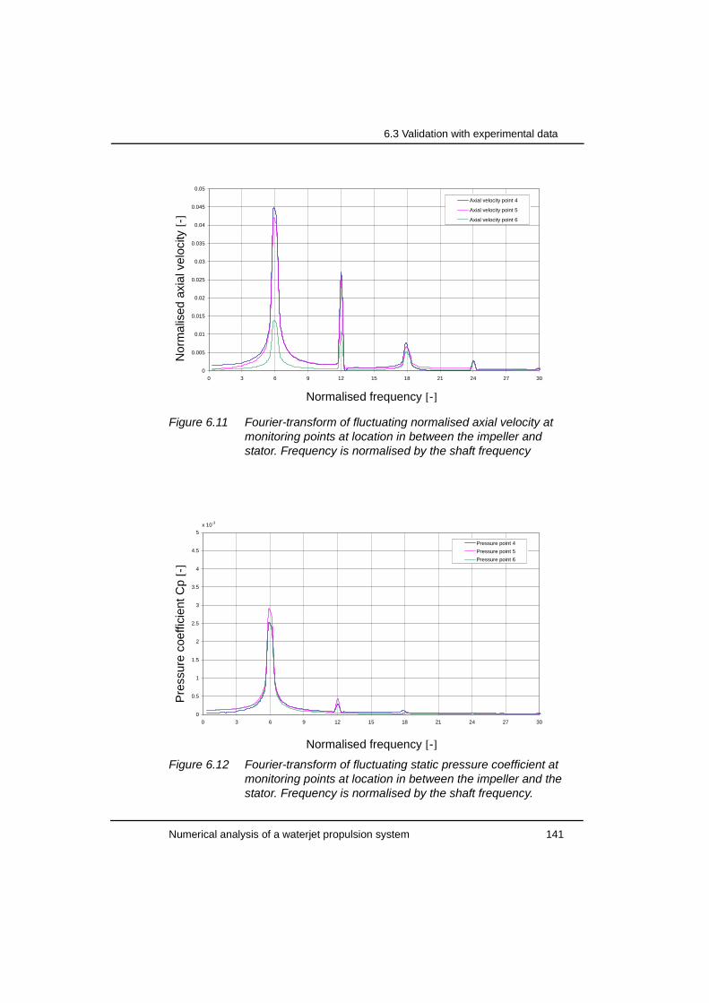
6.3 Validation with experimental data
Numerical analysis of a waterjet propulsion system 141
Figure 6.11 Fourier-transform of fluctuating normalised axial velocity at monitoring points at location in between the impeller and stator. Frequency is normalised by the shaft frequency
0
0.005
0.01
0.015
0.02
0.025
0.03
0.035
0.04
0.045
0.05
0 3 6 9 12 15 18 21 24 27 30
Axial velocity point 4
Axial velocity point 5
Axial velocity point 6
Normalised frequency [-]
Nor
mal
ised
axi
al v
eloc
ity [-
]
Figure 6.12 Fourier-transform of fluctuating static pressure coefficient at monitoring points at location in between the impeller and the stator. Frequency is normalised by the shaft frequency.
0
0.5
1
1.5
2
2.5
3
3.5
4
4.5
5
0 3 6 9 12 15 18 21 24 27 30
Pressure point 4
Pressure point 5
Pressure point 6
x 10-3
Normalised frequency [-]
Pre
ssur
e co
effic
ient
Cp
[-]

142
Chapter 6. Numerical analysis of waterjet pump flow
Performance diagrams
Transient flow calculations have been made for a number of flow rates. Thepump performance parameters, like head and torque are averaged over anumber of timesteps.
Figure 6.13 shows the mass averaged head curve based on equation (6.2)for both the quasi-steady and the transient flow calculations. Theexperimental data is plotted as reference.The results for the head curvesbased on the area averaged quantities, according to equation (6.4), is shownin figure 6.15.
Both methods show the tendency of a slight increase of the head for thetransient flow calculations. This phenomenon is also observed in calculationsbased on a potential flow method by Van Esch [9]. Agreement with theexperimental data is still acceptable for both the quasi-steady and thetransient flow calculations.
The comparison for the impeller torque is shown in figure 6.14. Bothnumerical methods as well as the experimental data are shown in this figure.A similar trend is seen for the torque as for the head, where transient flowresults show slightly higher values. The efficiency of the pump is shown infigure 6.16 for the quasi-steady and transient flow calculations. This efficiencyis based on the mass averaged head. It is observed that the transient flowcalculations predict a small increase of efficiency compared to the quasi-steady flow results.
Figure 6.13 Comparison of results of quasi-steady and transient flow calculations of mass averaged head based on equation (6.2)
0%
20%
40%
60%
80%
100%
120%
140%
160%
180%
200%
50% 60% 70% 80% 90% 100% 110% 120%
Measurements
CFD_quasi_steady
CFD_transient
Q/Qbep [%]
H/H
bep
[%]

6.3 Validation with experimental data
Numerical analysis of a waterjet propulsion system 143
Figure 6.14 Comparison of results of quasi-steady and transient flow calculations of area averaged head based on equation (6.4)
0%
20%
40%
60%
80%
100%
120%
140%
160%
180%
200%
50% 60% 70% 80% 90% 100% 110% 120%
Measurements
CFD_quasi_steady
CFD_transient
Q/Qbep [%]
H/H
bep
[%]
Figure 6.15 Comparison of results of quasi-steady and transient flow calculations of torque.
50%
60%
70%
80%
90%
100%
110%
120%
130%
140%
150%
50% 60% 70% 80% 90% 100% 110% 120%
Measurements
CFD_quasi_steady
CFD_transient
Q/Qbep [%]
T*/
T* b
ep [%
]

144
Chapter 6. Numerical analysis of waterjet pump flow
6.3.3 Rotor-stator interaction forces
The fully transient flow calculations with the moving mesh can be used toevaluate the radial force acting on the impeller due to rotor-stator interaction.Given the number of rotor and stator blades, an estimation of the behaviour ofthe interaction force can be made. The currently analysed configuration hassix rotor and seven stator blades. According to Brennen [10] and Dubas [11]this should give a radial force counter rotating at the blade passing frequency.
The counter rotating force is derived from a model which is based on theassumption of a variation in the pressure field when a rotating impeller bladepasses a stationary guide vane in the stator bowl. These fluctuations inpressure distribution result in a fluctuating force on the impeller. Disturbancesin the symmetry of the blade pressure distribution will result in a radial force.For this pump the angles between all the possible combinations of rotor andstator blade pairs are determined and inserted in a 6x7 matrix. Such a matrixcan be used to determine the sequence in which stator blades encounterpassing rotor blades. The resulting matrix is shown in table 6.1.
Realizing that angular distances decrease during rotation of the impeller, thesequence of stator blades with an impeller blade passing will be: 7 - 6 - 5 - 4 -3 - 2 - 1. The resulting interaction force has thus a counter-rotating directioncompared to the impeller rotation and can possibly lead to backward whirling.
Figure 6.16 Comparison of results of quasi-steady and transient calculations flow calculations of efficiency
50%
60%
70%
80%
90%
100%
110%
120%
50% 60% 70% 80% 90% 100% 110% 120%
Measurements
CFD_quasi_steady
CFD_transient
Q/Qbep [%]
η/η b
ep [%
]

6.3 Validation with experimental data
Numerical analysis of a waterjet propulsion system 145
Figure 6.17 shows the force map for different flowrates. The forces are madenon-dimensional to obtain the force coefficients Cfx and Cfy defined as:
(6.10)
The two force components are combined to get the radial force componentCfr1:
(6.11)
During the calculations, output is generated with a frequency of 960 Hz,which is equivalent to five times the blade passing frequency. The amount ofscatter of the force signal at each of these five points in subsequent cyclesgives an indication of the higher order fluctuations in the solution. The time-averaged magnitude of the radial force Cfr1 for each flow rate is plotted as acircle in the force map.
The forces show a periodic behaviour for all flow rates. The centre of theconcentric circles, which represent the time-averaged magnitude of the force,is located at the impeller axis. This means that the time-average of both thehorizontal component Cfx as well as the vertical component Cfy of theinteraction force diminish. This is in accordance with the expectations, givena situation with uniform axi-symmetrical inflow and outflow.
The average of the blade interaction force has a minimum value at the designcondition, denoted as 100% flow rate. This quantity increases with decreas-ing flow rate. However, at 60% of the design flow a significant reduction of themagnitude of the radial force is observed. This effect can be observed moreclearly in figure 6.18, where the time averaged magnitude Cfr1 of the rotor-
Table 6.1 Angular distance between rotor and stator blades forpump with 6 rotor blades and 7 stator blades
Stator1
Stator2
Stator3
Stator4
Stator5
Stator6
Stator7
Rotor1 0.0 51.4 102.9 154.3 205.7 257.1 308.6
Rotor2 300.0 351.4 42.9 94.3 145.7 197.1 248.6
Rotor3 240.0 291.4 342.9 34.3 85.7 137.1 188.6
Rotor4 180.0 231.4 282.9 334.3 25.7 77.1 128.6
Rotor5 120.0 171.4 222.9 274.3 325.7 17.1 68.6
Rotor6 60.0 111.4 162.9 214.3 265.7 317.1 8.6
CfxFx
ρΩ2D
4------------------= Cfy
Fy
ρΩ2D
4------------------=
Cfr1 Cfx2
Cfy2
+=

146
Chapter 6. Numerical analysis of waterjet pump flow
stator interaction force and the corresponding standard deviation are plottedas function of the flow rate. The standard deviation shows a minimum nearthe design point, which is in agreement with the expectations.
Figure 6.17 Plot of rotor-stator interaction force for different flow rates: instantaneous values (markers) and time-average of magnitude of force coefficient (dotted curves)
-0.6
-0.4
-0.2
0
0.2
0.4
0.6
-0.6 -0.4 -0.2 0 0.2 0.4 0.6
Radial force - 60% flow rate
Radial force - 70% flow rate
Radial force - 80% flow rate
Radial force - 90% flow rate
Radial force - 100% flow rate
Radial force - 110% flow rate
Time average - 60% flow rate
Time average - 70% flow rate
Time average - 80% flow rate
Time average - 90% flow rate
Time average - 100% flow rate
Time average - 110% flow rate
Cf y
[-]
Cfx [-]
0
0.05
0.1
0.15
0.2
0.25
0.3
0.35
0.4
50% 60% 70% 80% 90% 100% 110% 120%0
0.005
0.01
0.015
0.02
0.025
0.03
0.035
0.04
Time-averaged force
Standard deviation
Figure 6.18 Time averaged rotor-stator interaction force coefficient Cfr1 and standard deviation as function of the flow rate
Tim
e av
erag
ed r
adia
l for
ce c
oeffi
cien
t Cf r1
[
Q/Qbep [%]
Sta
ndar
d de
viat
ion
[-]

6.4 Influence of non-uniform axial inflow
Numerical analysis of a waterjet propulsion system 147
Model scale measurements on the same waterjet pump have confirmed thepresence of multiple local minima and maxima of the radial force [12]. Theseresults have not been published yet.
6.4 Influence of non-uniform axial inflow
The results discussed in the previous section are obtained for uniform inflowvelocity distributions. Waterjets operate in a strongly non-uniform inflowdistribution as described in chapter 3. The effect of a non-uniform velocitydistribution on the pump performance and the impeller forces will beinvestigated in more detail in this section. Four distributions are used in theanalysis, the measured distributions are shown in given in figures 5.13a to5.13d. The non-uniform velocity distributions are imposed as boundarycondition in the numerical analysis with the aid of a Fourier seriesapproximation of the velocity distribution, according to equation (3.2).
All calculations performed with the non-uniform inflow distribution are carriedout with the transient moving mesh option of the CFD method. Results of thetransient flow calculations for uniform inflow show a radial force due to rotor-stator interaction. This force originates from the interaction between theimpeller trailing edge and the statorblade leading edge. With a non-uniforminflow velocity distribution, an additional source for a radial force isintroduced, since the velocity distribution is not axi-symmetric.
First the pump performance for the non-uniform inflow conditions will bereviewed. In the remainder of this section the effects of the inflow on theradial forces will be analysed.
6.4.1 Pump performance for non-uniform inflow
The calculations with uniform inflow velocity already showed an interestingdifference between the two methods for the determination of the pump headbased on either mass-averaged or area-averaged quantities. For thecalculations for non-uniform inflow velocity distributions, the differencesbetween the results of these two methods may increase even more. Tables6.2 and 6.3 show the normalised pump performance for four different inflowconditions. The flow rate for all calculations is equal to the design flow rate.The values in the tables have been normalised with the result from thecorresponding calculation with a uniform inflow distribution and design flowrate of 100%.
The results of the method based on the mass-averaged total pressure areshown in table 6.2. It can be observed that the variations in both head andtorque are limited to less than two percent for all inflow conditions. Theefficiency shows a small decrease for increasing non-uniformity.
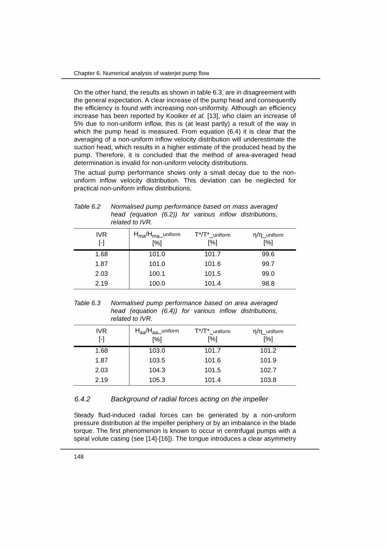
148
Chapter 6. Numerical analysis of waterjet pump flow
On the other hand, the results as shown in table 6.3, are in disagreement withthe general expectation. A clear increase of the pump head and consequentlythe efficiency is found with increasing non-uniformity. Although an efficiencyincrease has been reported by Kooiker et al. [13], who claim an increase of5% due to non-uniform inflow, this is (at least partly) a result of the way inwhich the pump head is measured. From equation (6.4) it is clear that theaveraging of a non-uniform inflow velocity distribution will underestimate thesuction head, which results in a higher estimate of the produced head by thepump. Therefore, it is concluded that the method of area-averaged headdetermination is invalid for non-uniform velocity distributions.
The actual pump performance shows only a small decay due to the non-uniform inflow velocity distribution. This deviation can be neglected forpractical non-uniform inflow distributions.
6.4.2 Background of radial forces acting on the impeller
Steady fluid-induced radial forces can be generated by a non-uniformpressure distribution at the impeller periphery or by an imbalance in the bladetorque. The first phenomenon is known to occur in centrifugal pumps with aspiral volute casing (see [14]-[16]). The tongue introduces a clear asymmetry
Table 6.2 Normalised pump performance based on mass averagedhead (equation (6.2)) for various inflow distributions,related to IVR.
IVR[-]
Hma/Hma_uniform [%]
T*/T*_uniform
[%]η/η_uniform
[%]
1.68 101.0 101.7 99.6
1.87 101.0 101.6 99.7
2.03 100.1 101.5 99.0
2.19 100.0 101.4 98.8
Table 6.3 Normalised pump performance based on area averagedhead (equation (6.4)) for various inflow distributions,related to IVR.
IVR[-]
Haa/Haa_uniform [%]
T*/T*_uniform
[%]η/η_uniform
[%]
1.68 103.0 101.7 101.2
1.87 103.5 101.6 101.9
2.03 104.3 101.5 102.7
2.19 105.3 101.4 103.8

6.4 Influence of non-uniform axial inflow
Numerical analysis of a waterjet propulsion system 149
in the geometry. Waterjet installations with a stator bowl do not suffer fromsuch type of a-symmetry, however. This source for a radial force cantherefore be excluded. The non-uniform inflow velocity may create a non-symmetrical pressure distribution on the hub surface. This may result in a netradial force.
Imbalance in blade torque may give a more significant contribution to theradial forces acting on the impeller. The concept of this imbalance is shown infigure 6.19.
Non-uniformity of the inflow velocity distribution will result during a revolutionin variations of both the flow angle at the leading edge and the flow ratethrough an impeller channel. This will result in a torque contribution that isdifferent for each blade. The difference in torque contributions between twoopposite blades will result in a net radial force on the impeller axis.
6.4.3 Flow rate fluctuations in the impeller channel
The CFD results are used to determine the local flow rate Qbb through theimpeller channel between two consecutive blades. The volume flow rate isdetermined at a cross-sectional plane at mid-chord of the impeller blades.Figure 6.20 shows the normalized local flow rate as a function of the rotorposition for the four different inflow conditions.
Even for the case of maximum level of non-uniformity, i.e. for IVR=2.19, themaximum deviation is less than 7% of the average. The variations obtainedfrom the CFD results are much smaller than the predictions based on theanalytical approach used in section 3.2. It appears that the non-uniform inflowvelocity distribution is smoothed in the first part of the pump. This willinfluence the local flow angles at the leading edge of the impeller blade. As aconsequence, the blade loading and the blade torque will be influenced. Thiseliminates the possibility to derive a simple analytical model to estimate theradial and tangential forces on the impeller.
Figure 6.19 Concept of radial force due to unbalanced blade torque
net radial force

150
Chapter 6. Numerical analysis of waterjet pump flow
6.4.4 Radial forces for non-uniform inflow
The non-uniform inflow velocity distribution has an effect on the radial forcesacting on the impeller. For a uniform inflow distribution a periodic rotor-statorinteraction force is found, as shown in subsection 6.3.3. In this section theforces are evaluated that are caused by the non-uniformity of the inflow.
Figure 6.22 shows a graph of the horizontal and vertical component of theforce acting on the impeller for different IVR, each with a typical non-uniforminflow velocity distribution, at the design flow rate.
The forces acting on the impeller can be approximated by a mean componentCfr0 and harmonic components Cfr1 and Cfr2:
(6.12)
This is shown in a sketch in figure 6.21 for the mean component Cfr0 and thefirst harmonic Cfr1.
90%
92%
94%
96%
98%
100%
102%
104%
106%
108%
110%
0 45 90 135 180 225 270 315 360
IVR = 1.68
IVR = 1.87
IVR = 2.03
IVR = 2.19
Figure 6.20 Normalised channel flow rate Qbb as a function of the rotor position for various inflow distributions, which are related to the IVR
Angle θ [degrees]
Qbb
/(Q
/N)
[%]
Cfr Cfr0 Cfr1 ωt⋅ Cfr2 2ωt⋅+ +=

6.4 Influence of non-uniform axial inflow
Numerical analysis of a waterjet propulsion system 151
From the results as presented in figure 6.22 can be seen that the mean radialcomponent Cfr0 shows a strong relation with the level of non-uniformity, whichis in accordance with expectations. The direction of the mean force seems tobe constant for all inflow conditions. This direction may be related to the flowrate through the pump, which is equal for all presented conditions in figure6.22.
The condition with the most severe non-uniform velocity distribution (IVR =2.19) shows quite some scatter of the time dependent force. This seems tobe an indication of higher order harmonics (i.e. Cfr2 and Cfr3) in the system atthese inflow conditions.
Figure 6.21 Sketch of radial forces acting on the impeller due to non-uniform inflow.
x
y
Cfr0
Cfr1 ω
-1
0
1
2
3
4
5
-1 0 1 2 3 4 5 6 7 8
Uniform inflow
IVR = 1.68
IVR = 1.87
IVR = 2.03
IVR = 2.19
x 10-3
x 10-3
Figure 6.22 Horizontal and vertical component of time-dependent impeller force coefficient for different inflow velocity distributions, which are related to IVR, at design flow rate
Horizontal force coefficient Cfx [-]
Ver
tical
forc
e co
effic
ient
Cf y
[-]

152
Chapter 6. Numerical analysis of waterjet pump flow
Figure 6.23 shows the plot of the forces for 80% of the design flow rate. Theoccurrence of increasing mean force Cfr0 with increasing non-uniformity isconfirmed. The magnitude of both the mean force Cfr0 and the first harmonicCfr1 are different compared to the results for 100% flow rate. Moreover, thedirection of the steady force has changed for this flow rate.
Analysis of mean radial force Cfr0The results of the calculations for different flow rates and levels of non-uniformities show that both parameters influence the mean radial force Cfr0.A quantitative assessment is made in table 6.4, where the time averagedmagnitude and the direction of the non-dimensional radial force are listed.The direction angle α is calculated according to:
(6.13)
The direction of the radial force shows a small increase with increasing non-uniformity. Results at the design capacity show a variation of less than 1.5degrees. On the other hand, the differences due to variation in flow rate aresignificant. At an IVR of 2.03 a deviation of 4.6 (= 30.5 - 25.9) degrees isfound.
-1
0
1
2
3
4
5
-1 0 1 2 3 4 5 6 7 8
Uniform inflow
IVR = 1.68
IVR = 1.87
IVR = 2.03
IVR = 2.19
x 10-3
x 10-3
Figure 6.23 Horizontal and vertical component of time-dependent impeller force coefficient for different inflow velocity distributions, which are related to IVR, at 80% of the design flow rate
Horizontal force coefficient Cfx [-]
Ver
tical
forc
e co
effic
ient
Cf y
[-]
αCfyCfx--------
atan=

6.4 Influence of non-uniform axial inflow
Numerical analysis of a waterjet propulsion system 153
The variation in direction seems to be related to the flow rate. This may bedue to an increase of the residence time of the fluid in the impeller, in whichthe impeller will rotate over a larger angle. The direction of the radial force willrotate accordingly.
Analysis of unsteady forces
The unsteady radial force can be examined in more detail, if the mean forcecomponents Cfx0 and Cfy0 are subtracted from the results. The resultant ofthe vertical and horizontal component is plotted in figure 6.24 for the designflow rate and in figure 6.24 for 80% of design flow rate.
The results of the calculations with uniform inflow indicate a rotating radialforce with a mean magnitude. The condition with the highest level of non-uniformity at design flow rate shows a chaotic behaviour of the unsteadyforces. This is a result of higher order fluctuations of the forces.
At 80% of design flow rate, the behaviour of the fluctuating forces is moreregular. Figure 6.24 shows that the shape of the locus of the forcecomponents becomes more and more elliptical, when the level of non-uniformity is increased. This means that the higher order harmonics of theradial force, i.e. Cfr2 and Cfr3, become more important for these conditions.
This is confirmed by the Fourier transformation of the fluctuating componentof the radial force, as shown in figure 6.26. The conditions at 80% of thedesign flow rate and at the design flow rate and moderate levels of non-uniformity show two clear peaks at one and two times the blade passing
Table 6.4 Time-averaged magnitude Cfr0 and direction α of radialforce coefficient
Flow rate IVR Cfr0*1000 α
100% 1.68 3.819 24.9
100% 1.87 4.569 25.3
100% 2.03 5.550 25.9
100% 2.19 6.478 26.2
80% 1.68 2.368 28.9
80% 1.87 2.826 29.7
80% 2.03 3.423 30.5
80% 2.19 3.977 31.3

154
Chapter 6. Numerical analysis of waterjet pump flow
frequency. The conditions at design flow rate and an IVR above 2 shownumerous additional peaks at other frequencies. This is represented in thechaotic behaviour of the radial force.
-0.4
-0.3
-0.2
-0.1
0
0.1
0.2
0.3
0.4
-0.6 -0.5 -0.4 -0.3 -0.2 -0.1 0 0.1 0.2 0.3 0.4 0.5 0.6
Uniform inflow
Curve-fit
IVR = 1.68
IVR = 1.87
IVR = 2.03
IVR = 2.19
x 10-3
x 10-3
Figure 6.24 Unsteady impeller force components for different inflow velocity distributions at design flow rate.
Horizontal force Cfx-Cfx0 [-]
Ver
tical
forc
e C
f y-C
f y0
[-]
-0.4
-0.3
-0.2
-0.1
0
0.1
0.2
0.3
0.4
-0.6 -0.5 -0.4 -0.3 -0.2 -0.1 0 0.1 0.2 0.3 0.4 0.5 0.6
Uniform inflow
Curve-fit
IVR = 1.68
IVR = 1.87
IVR = 2.03
IVR = 2.19
x 10-3
x 10-3
Figure 6.25 Unsteady impeller force components for different inflow velocity distributions at 80% of design flow rate.
Horizontal force Cfx-Cfx0 [-]
Ver
tical
forc
e C
f y-C
f y0
[-]
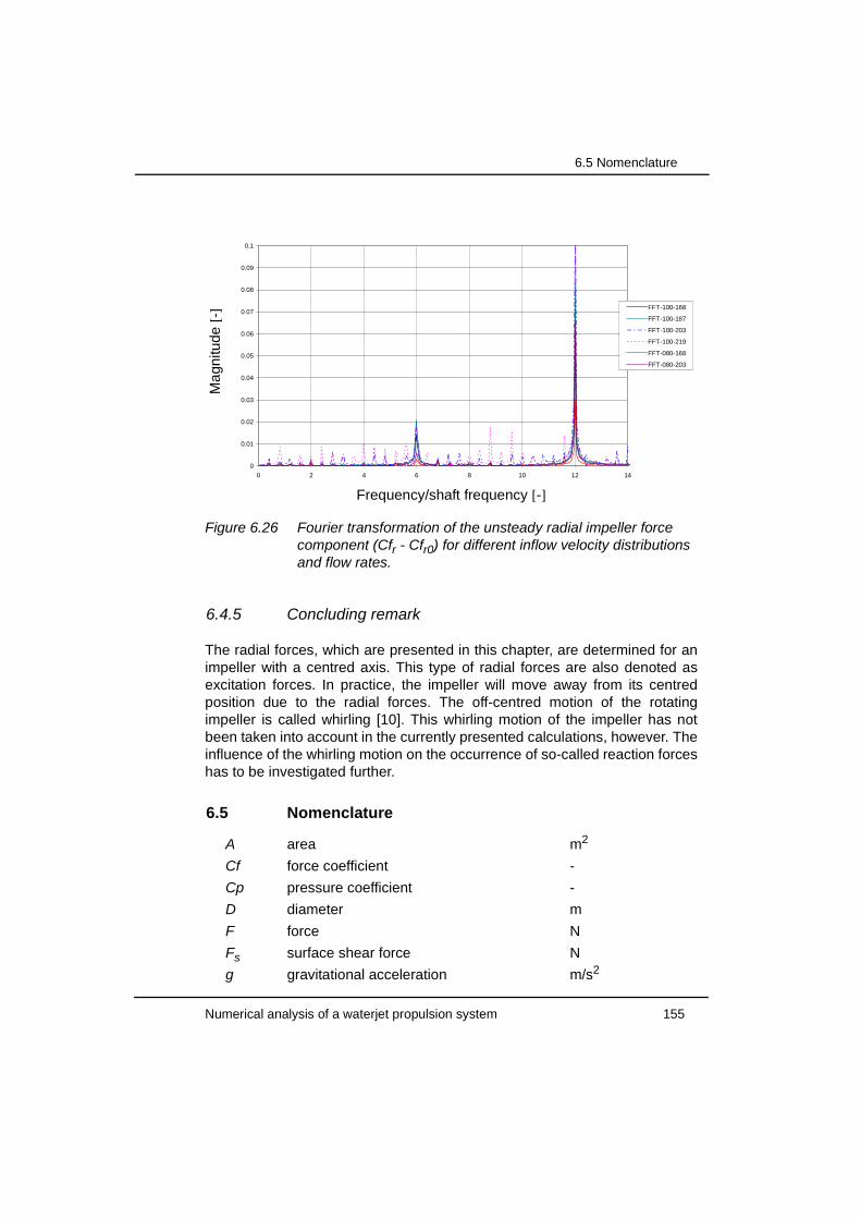
6.5 Nomenclature
Numerical analysis of a waterjet propulsion system 155
6.4.5 Concluding remark
The radial forces, which are presented in this chapter, are determined for animpeller with a centred axis. This type of radial forces are also denoted asexcitation forces. In practice, the impeller will move away from its centredposition due to the radial forces. The off-centred motion of the rotatingimpeller is called whirling [10]. This whirling motion of the impeller has notbeen taken into account in the currently presented calculations, however. Theinfluence of the whirling motion on the occurrence of so-called reaction forceshas to be investigated further.
6.5 Nomenclature
A area m2
Cf force coefficient -
Cp pressure coefficient -
D diameter m
F force N
Fs surface shear force N
g gravitational acceleration m/s2
0
0.01
0.02
0.03
0.04
0.05
0.06
0.07
0.08
0.09
0.1
0 2 4 6 8 10 12 14
FFT-100-168
FFT-100-187
FFT-100-203
FFT-100-219
FFT-080-168
FFT-080-203
Figure 6.26 Fourier transformation of the unsteady radial impeller force component (Cfr - Cfr0) for different inflow velocity distributions and flow rates.
Frequency/shaft frequency [-]
Mag
nitu
de [-
]

156
Chapter 6. Numerical analysis of waterjet pump flow
H head m
pstat static pressure Pa
ptot total pressure Pa
Q flow rate m3/s
r radial distance m
T* torque coefficient -
T torque Nm
vn normal velocity m/s
Greek symbols
α radial force direction deg
ρ density kg/m3
Ω shaft speed rad/s
Subscripts
in inlet plane
n normal direction
out outlet plane
r0 mean component of radial force coefficient
r1, r2 harmonics of rotor-stator interaction force coefficient
t tangential direction
x horizontal direction
y vertical direction
6.6 References
[1] Goto, A., ‘Study of internal flows in a mixed-flow pump impeller at vari-ous tip clearances using three-dimensional viscous flow computations’,Journal of Turbomachinery, Vol 114, pp. 373-382, 1992
[2] Nilson, H., Davidson, L., ‘A numerical comparison of four operatingconditions in a Kaplan water turbine, focusing on tip clearance flow’,Proceedings 20th IAHR symposium, Charlotte, 2000
[3] Aschenbrenner, T., Göhringer, M., Moser, W., ‘Numerical and experi-mental flow analysis in a Kaplan turbine’, Proceedings 20th IAHR sym-posium, Charlotte, 2000
[4] Kunz, R.F., Lakshminarayana, B., Basson, A.H., ‘Investigation of tipclearance phenomena in an axial compressor cascade using Euler and

6.6 References
Numerical analysis of a waterjet propulsion system 157
Navier-Stokes procedures, Journal of Turbomachinery, Vol 115, pp.453-467, 1993
[5] Versteeg, H.K. & Malalasekera, W., ‘An introduction to ComputationalFluid Dynamics’, Longman Scientific & Technical, Essex, 1995
[6] Fox, R.W., & McDonald, A.T.,’Introduction to fluid mechanics’, ThirdEdition, John Wiley & Sons, New York, 1985
[7] Gülich, J.F., Favre, J.N., Denus, K., ’An assessment of pump impellerperformance predictions by 3D-Navier Stokes calculations’, ASME Flu-ids Engineering Division summer meeting, 1997
[8] Cugal, M., Baché, G., ’Performance prediction from shutoff to runoutflows for a complete stage of a boiler feed pump using computationalfluid dynamics’, ASME Fluids Engineering Division summer meeting,1997
[9] Van Esch, B.P.M.,’Simulation of three-dimensional unsteady flow inhydraulic pumps’, PhD thesis, University of Twente, 1997
[10] Brennen, C.E., 'Hydrodynamics of pumps', Oxford University Press,1994
[11] Dubas, M., ‘Über die Erregung infolge der Periodizität von Turboma-chinen’, Ingenieur-Archiv, vol. 54, pp. 413-426., 1984
[12] Esch, B.P.M. van, personal communication.
[13] Kooiker, K., Van Terwisga, T., Verbeek R., Van Terwisga, P., 'Perform-ance and cavitation analysis of a waterjet system on a cavitation tun-nel', proceedings FAST 2003 conference, session A1 pp 57-62, Ischia,Italy, 2003
[14] Stepanoff, A.J., “Centrifugal and axial flow pumps - Theory, design andapplication”, 2nd edition, John Wiley, 1964
[15] Badie, R., ‘Analysis of unsteady potential flows in centrifugal pumps’,PhD thesis, University of Twente, 1993
[16] Jonker, J.B. & Van Essen, T.G., ‘A finite element pertubation methodfor computing fluid-induced forces on a centrifugal impeller rotating in avolute casing’, International journal for numerical methods in engineer-ing, Vol. 40, pp. 269-294, 1997

158
Chapter 6. Numerical analysis of waterjet pump flow

Numerical analysis of a waterjet propulsion system 159
Chapter 7 Analysis of a complete waterjet installation
In the preceding two chapters the waterjet inlet and the mixed-flow pumpwere analysed separately. In this chapter the complete waterjet installation isconsidered. Results are presented of the numerical analysis of such apropulsion system on full scale. An analysis is made of the overallperformance indicators, like volume flow rate, thrust and power. Comparisonsare made with performance prediction and selection software of WärtsiläPropulsion Netherlands (WPNL-select). This software is partially based onsemi-empirical relations, which are tuned to the performance of thepropulsion systems in the currently sailing fleet.
A detailed analysis of the streamtube will reveal some new insights into theforces acting on the installation in both vertical and axial direction.
7.1 Generation of the numerical model
The numerical domain of the complete waterjet installation is a combinationof the two separate grids of the waterjet inlet and the mixed-flow pump. Theinterface between the two grids is located at the cross-section down-streamof the inlet bend (see figure 5.1 for the location of these parts). At thisinterface a coupling method is used to create a fully connected domain,based on arbitrary matching of the cells. It should be noted that this interfacebetween the models of the inlet and the pump is different from the two slidinginterfaces, which are required for the rotation of the impeller.
Care should be taken that the dimension of the nozzle exit area is equal tothe exit area of the actual full-scale installation. The sensitivity of the flow rate

160
Chapter 7. Analysis of a complete waterjet installation
as function of the nozzle size has been illustrated in figure 2.8 on page 36.Figure 7.1 shows a plot of the final mesh of the full scale waterjet installation.
The boundary conditions and parameters of the numerical method areidentical to the ones used for the calculations of the separate parts. At theinlet side of the domain a prescribed velocity distribution is applied, with aboundary layer velocity profile. At the other sides on the domain beneath thehull and at the nozzle exit plane constant pressure boundary conditions areapplied. As a consequence, the actual flow rate through the waterjetbecomes a part of the solution, whereas it was prescribed by the boundaryconditions in the calculations for the isolated inlet and pump.
7.2 Evaluation of volume flow rate
The calculations are made with a constant rotational speed of the pump and avarying ship speed. In this way a relatively large range of IVR conditions iscovered. The variation in volume flow rate will be much smaller, as indicatedby the results presented in figure 2.9 on page 37.
The calculated volume flow rate through the waterjet is compared with theresults of WPNL-select. To a large extent, this program is based on the theoryas discussed in chapter 2. The loss coefficients in this method are empiricalvalues taken from experimental data. Further fine-tuning is made withadditional empirical data. The accuracy of the method is continuouslyincreased by adding the measured performance of newly installed waterjetinstallations. Since the currently sailing fleet performs according to the
Figure 7.1 Mesh of the complete waterjet installation, number of cells is about 1.2 million.
inlet side
nozzle exit
pump
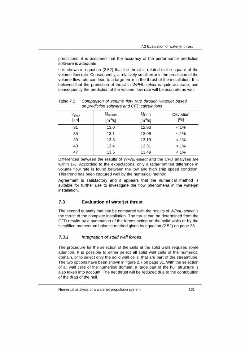
7.3 Evaluation of waterjet thrust
Numercal analysis of a waterjet propulsion system 161
predictions, it is assumed that the accuracy of the performance predictionsoftware is adequate.
It is shown in equation (2.52) that the thrust is related to the square of thevolume flow rate. Consequently, a relatively small error in the prediction of thevolume flow rate can lead to a large error in the thrust of the installation. It isbelieved that the prediction of thrust in WPNL-select is quite accurate, andconsequently the prediction of the volume flow rate will be accurate as well.
Differences between the results of WPNL-select and the CFD analyses arewithin 1%. According to the expectations, only a rather limited difference involume flow rate is found between the low and high ship speed condition.This trend has been captured well by the numerical method.
Agreement is satisfactory and it appears that the numerical method issuitable for further use to investigate the flow phenomena in the waterjetinstallation.
7.3 Evaluation of waterjet thrust
The second quantity that can be compared with the results of WPNL-select isthe thrust of the complete installation. The thrust can be determined from theCFD results by a summation of the forces acting on the solid walls or by thesimplified momentum balance method given by equation (2.52) on page 33.
7.3.1 Integration of solid wall forces
The procedure for the selection of the cells at the solid walls requires someattention. It is possible to either select all solid wall cells of the numericaldomain, or to select only the solid wall cells, that are part of the streamtube.The two options have been shown in figure 2.7 on page 31. With the selectionof all wall cells of the numerical domain, a large part of the hull structure isalso taken into account. The net thrust will be reduced due to the contributionof the drag of the hull.
Table 7.1 Comparison of volume flow rate through waterjet basedon prediction software and CFD calculations
vship[kn]
Qselect
[m3/s]
QCFD
[m3/s]Deviation
[%]
31 13.0 12.93 < 1%
35 13.1 13.08 < 1%
39 13.3 13.19 < 1%
43 13.4 13.31 < 1%
47 13.6 13.49 < 1%

162
Chapter 7. Analysis of a complete waterjet installation
Selection of the solid wall cells of the streamtube only, can not be done with awell-defined procedure, however. The wall cells near the streamtube surfacewill be partly included in the streamtube. The results show a significantinfluence of the choice whether these cells are included or excluded from theselection. The process of wall cell selection is avoided, when all solid wallcells of the numerical domain are taken into account in the force evaluation.The additional drag of the hull structure can be compensated for, given thedimensions of the numerical domain.
The method using drag compensation is also preferable from a ship builder’spoint of view. This is due to a subtle difference between a vessel with waterjetpropulsion and a vessel with conventional propeller propulsion. For such apropeller ship, the hull and the propeller can be split into two subsystems. Awaterjet propelled vessel can not be split into a bare hull and a propulsionunit, without leaving a hole in the hull structure. In a bare hull resistance test,additional hull drag, due to the development of the boundary layer, will bemeasured at the location of the inlet duct opening. The additional drag of theboundary layer will change once the waterjet installation with the inlet duct isinstalled.
It is concluded that the thrust of the installation has to be computed using allsolid wall cells and that frictional resistance of the original hull area has to becompensated for. The total waterjet thrust is then:
(7.1)
where Twj,all is the integrated force of the pressure and wall friction on all solidwall cells and Dhull the drag force of the equivalent rectangular hull area.
Calculation of the drag of the hull boundary layer is based on flat plateboundary layer theory for high Reynolds numbers. This formula is used,because it is also used to extrapolate model scale bare hull resistance data tofull scale predictions. The friction coefficient is given by [1]:
(7.2)
where the friction coefficient Cf is defined as:
(7.3)
with Dhull the actual friction drag of the equivalent hull, vship the undisturbedvelocity, and Ahull the area of the equivalent hull, which is length times widthof the used mesh.
Twj Twj all, Dhull–=
Cf0.455
Rel( )2.58log--------------------------------=
Cf
Dhull
12---ρvship
2Ahull
---------------------------------=

7.3 Evaluation of waterjet thrust
Numercal analysis of a waterjet propulsion system 163
The Reynolds number for the flat plate is defined as:
(7.4)
where Lwetted is the wetted length of the hull upstream of the inlet. The actualdrag of the hull area of the numerical domain depends on the dimensions ofthe area A and the wetted length of the hull upstream of the waterjet inlet.
7.3.2 Momentum balance
The thrust based on the momentum balance, can be calculated with thesimplified equation (2.52). In this equation the contribution of the pressuredistribution on the streamtube below the hull and the aft part of the hull isneglected. The introduced error can be compensated with the so-called thrustdeduction factor tj [2]. The mass averaged inflow velocity is determined usinga concentration scalar as described in detail in section 5.5.
7.3.3 Results
Figure 7.2 shows the thrust of the full-scale installation based on WPNL-select and on the CFD calculations. In order to show the differences betweenresults of the two methods that use the results of the CFD calculations, asdescribed above, both results are presented in the graph. The results havebeen normalised with the design thrust at a ship speed of 39 knots.
The method of integration of the solid wall forces shows a very goodagreement with the prediction software for the ship speeds up to 39 knots,which is the design speed for the investigated installation. At higher speeds asmall difference is found between the results of the force integration methodand the results of the prediction software.
The method based on the momentum balance gives a good agreement up toship speeds of 35 knots. At higher speeds the momentum balance gives alower thrust than the force integration and the prediction software.
The deviations between the results of the two numerical methods are quitesignificant at higher ship speeds. This phenomenon may be attributed tonumerical inaccuracies.
However, it can also be an indication that the simplification of the momentumbalance is the cause for this, as discussed in subsection 2.3.3 at page 30. Itis known, that the low pressure region along the cutwater will have a positivecontribution to the thrust. This may explain the deviations found between theresults of the force integration method based on considering the pressure andshear stress on all solid wall cells and the ones of the momentum balanceapproach, which is applied to the streamtube.
Rel
ρvshipLwetted
µ------------------------------------=

164
Chapter 7. Analysis of a complete waterjet installation
7.4 Evaluation of required power
Evaluation of the required power is equivalent to the evaluation of therequired torque, since all calculations have been made at the same rotationalspeed. The torque is obtained from the summation of the torque of the solidwall cells of the impeller. The resulting torque is multiplied by the angularvelocity of the impeller to obtain the required power.
Figure 7.3 shows the power based on the calculations and the one obtainedfrom the prediction software. Results are normalised with the required powerof the full scale installation at the design speed computed with the predictionsoftware. Over the complete range of calculated conditions, a small over-prediction of the power can be observed. The deviation of about 2.5% isacceptable, however. The deviation is more or less constant for all conditions,due to the very small variation in flow rate. The increase in flow rate is only4.5% for an increase of ship speed from 31 to 47 knots.
Figure 7.2 Comparison of thrust of waterjet installation based on WPNL-select with numerical predictions based on force integration of solid wall forces (Twj) and momentum balance applied to the streamtube (equation (2.52)).
80%
85%
90%
95%
100%
105%
110%
115%
120%
30 32 34 36 38 40 42 44 46 48
Prediction software
Integration of solid wall forces
Momentum balance
Ship speed [knots]
Thr
ust/T
hrus
t 39
knot
s [-
]

7.5 Analysis of vertical force on waterjet structure
Numercal analysis of a waterjet propulsion system 165
7.5 Analysis of vertical force on waterjet structure
In the preceding section, the prediction of the waterjet thrust is discussed.While calculating the thrust of the waterjet installation, based on theintegration of the forces acting on the solid walls, it is found that there can bea net force in the vertical direction as well. This vertical force component is infact a lift force acting on the waterjet structure.
This result of the numerical analysis is not in agreement with the results ofVan Terwisga [2], who claims that there is no net lift contribution. On the otherhand, Svensson [3] determined a lift force from pressure measurements inthe intake and on the hull, which can be up to 5% of the displacement of thevessel.
Applying equation (2.35) for the vertical direction yields:
(7.5)
where Lwj is a vertical force on either the waterjet or the hull. The verticalcomponents of the momentum fluxes do not contribute, since it is assumed
90.0%
92.5%
95.0%
97.5%
100.0%
102.5%
105.0%
107.5%
110.0%
30 32 34 36 38 40 42 44 46 48
Prediction software
CFD result
Figure 7.3 Comparison of required power of waterjet installation obtained from prediction software and the one obtained from CFD calculations
Ship speed [knots]
Pow
er/P
ower
39 k
nots
[-]
Lwj all, pz Ad⋅Atube
∫– Lwj hull,+=
166
Chapter 7. Analysis of a complete waterjet installation
that both the velocity distributions at the inlet and nozzle exit are aligned withthe horizontal direction.
A more detailed analysis of the occurring lift force coefficient, reveals that thelargest lift is found at high IVR conditions, and therefore high ship speed. Thenumerical results presented in this subsection are for a waterjet installationfor very high speed vessels. The most important difference fromhydrodynamic point of view between a conventional waterjet installation anda high-speed application is found in the geometry of the inlet duct [4].
Inlet lift coefficient
The actual lift force acting on the inlet structure is presented as a non-dimensional coefficient, according to:
(7.6)
where Lwj,all is the calculated vertical force, ρ the density, Q the volume flowand vpump the averaged axial velocity upstream of the impeller. The liftcoefficient is plotted as a function of IVR in figure 7.4.
Up to an IVR of about 1.5 the lift coefficient is indeed rather small. For highspeed applications (>60 knots) the IVR will be about 2 to 2.2. This will resultin a lift coefficient of about 0.08 to 0.10.
Equation (7.6) can be expressed in specific pump parameters Ω, D and ϕ aswell with equation (2.15) as:
(7.7)
The second factor on the right hand side is of order 1 for common waterjetmixed-flow pumps. Thus, a direct comparison between the lift forcecoefficient on the inlet and the vertical force coefficient on the impeller, as aresult of non-uniformity can be made. At an IVR of 2.19, the vertical force is
about 2.85x10⁻³, according to figure 6.22 on page 151. The vertical forcecoefficient in the inlet for that condition is 0.081, based on figure 7.4. It isconcluded that the vertical force in the inlet is significantly larger (almostfactor 30) than the vertical component of the impeller force due to non-uniform inflow velocity distributions.
CL
Lwj all,
ρQvpump-----------------------=
CL
Lwj all,
ρΩ2D
4------------------ π
4ϕ2---------⋅=

7.5 Analysis of vertical force on waterjet structure
Numercal analysis of a waterjet propulsion system 167
Inlet lift-thrust ratio
The lift force can also be compared to the thrust of the waterjet installation.The thrust of a waterjet can be rewritten from equation (2.52), with aid ofequations (2.2), (2.11), (2.12) and (2.13) to:
(7.8)
where Dinlet and Dnozzle are two geometric parameter of the installation and wis the wake fraction, defined in equation (2.2).
The lift-thrust ratio becomes:
(7.9)
This shows that the lift-thrust ratio is related to the lift coefficient, the wakefraction and the geometry of the waterjet installation. The data for the liftcoefficient as shown in figure 7.4 is presented as lift-thrust ratio in figure 7.5.
Figure 7.4 Lift coefficient CL as a function of IVR
-0.05
0
0.05
0.1
0.15
0.2
0.25
0 0.5 1 1.5 2 2.5
Lift force coefficient
IVR [-]
CL
[-]
T ρQvpump
Dinlet
Dnozzle------------------
21 w–( ) IVR⋅–
=
LT---
CL
Dinlet
Dnozzle------------------
21 w–( ) IVR⋅–
------------------------------------------------------------------------=

168
Chapter 7. Analysis of a complete waterjet installation
Since the thrust decreases with increasing IVR, the lift-thrust ratio shows asteep increase at high values of IVR: a significant lift force of about 10-20% ofthe thrust is found. This amount of lift can not be neglected in general.
The lift force in the inlet creates a moment on the hull structure at highspeeds, which can lead to a reduced or even negative trim angle of thevessel.
7.6 Pressure distribution on streamtube surface
7.6.1 Evaluation of momentum balance in vertical direction
The CFD analyses reveal the presence of a significant lift force in a waterjetinstallation at the higher IVR conditions. Based on equation (7.5), the lift canbe the result of a net force acting on the hull surface or of a resultant force ofthe pressure distribution, which acts on the streamtube surface.
These two terms are neglected in the standard momentum theory, which is inaccordance with the simplified thrust equation (2.52). As a result, the net liftforce is equal to zero for all conditions.
The contribution of the vertical forces acting on the hull surface are limited toa region near the cutwater. It is known from CFD analyses that the pressurein this region is very low for high IVR conditions (see for example figure 5.6).It is expected that any possible contribution to the vertical force will be anegative lift for high IVR. It is concluded that the lift force on the complete
-5%
0%
5%
10%
15%
20%
25%
0 0.5 1 1.5 2 2.5
Lift-thrust ratio
Figure 7.5 Lift-thrust ratio L/T as a function of IVR
IVR [-]
L/T
[-]

7.6 Pressure distribution on streamtube surface
Numercal analysis of a waterjet propulsion system 169
waterjet structure, should originate from a pressure distribution along thestreamtube surface. A method to integrate the pressure distribution on thestreamtube surface is required to confirm this.
Accurate determination of the lift force, acting on the hull structure, is notpossible with the applied method. It is not possible to determine thecontribution of the solid wall cells near the streamtube interface accurately,because the effect of partially included solid wall cells can not be taken intoaccount.
The shape of the streamtube depends on the IVR at which the waterjetoperates. The pressure distribution also depends on IVR. In order todetermine the net force, an integration of the pressure over the surface has tobe made. For this numerical integration, the surface of the streamtube issubdivided into triangles, based on the Delaunay triangularisation method.The net lift force can be determined, given the average pressure on eachtriangle and the normal direction.
7.6.2 Calculation of vertical force on streamtube
The streamtube shape is determined for various operating conditions of thehigh-speed waterjet installation, as discussed in the preceding section. Anexample of the triangular mesh of the streamtube surface is shown in figure7.6. The triangular mesh represents the streamtube surface and therectangular cells represent the solid wall cells of the waterjet inlet.
The resulting lift force of the streamtube pressure distribution is shown infigure 7.7. The force has been made non-dimensional according to equation(7.6).
The force of the integrated pressure distribution clearly depends on IVR. Atvalues of an IVR above 1.8 the net lift force on the streamtube exceeds thetotal lift force on the inlet. At these IVR conditions, the net force on the hull(near the cutwater) will be negative. This confirms the hypothesis of thecontribution of negative lift of the wall cells near the cut water at higher valuesof IVR. At an IVR of about 1.0 the net force on the cutwater region will bepositive, which is in agreement with expectations as well.

170
Chapter 7. Analysis of a complete waterjet installation
Figure 7.6 Example of triangular surface mesh of streamtube surface (in green). Rectangular cells represent solid wall cells of waterjet inlet in blue.
-0.15
-0.1
-0.05
0
0.05
0.1
0.15
0.2
0.25
0.3
0.35
0.4
0 0.5 1 1.5 2 2.5
Streamtube lift coefficient
Inlet lift coefficient
Figure 7.7 Lift force coefficient of streamtube pressure distribution as function of IVR compared to inlet lift coefficient
IVR [-]
CL
[-]

7.7 Nomenclature
Numercal analysis of a waterjet propulsion system 171
7.6.3 Concluding remark
A first attempt to quantify the forces, which result from the pressuredistribution along the streamtube, has shown that there can be a significantforce in vertical direction. This force depends on the value of the IVR of thewaterjet installation. However, the actual geometry of the inlet geometrymight have an important influence on the magnitude of the lift force as well.Further research of this is recommended before general conclusions can bedrawn.
7.7 Nomenclature
A area m2
Cf friction coefficient -
CL lift coefficient -
D diameter m
D drag force N
IVR inlet velocity ratio -
L length of flat plate m
L lift force N
p static pressure Pa
Q flow rate m3/s
T thrust N
v velocity m/s
w wake fraction -
z vertical direction
Greek symbols
µ dynamic viscosity kg/ms
ρ density kg/m3
ϕ flow coefficient -
Ω angular velocity rad/s
Subscripts
inlet inlet plane
nozzle nozzle exit plane
pump pump entrance plane
wj waterjet

172
Chapter 7. Analysis of a complete waterjet installation
7.8 References
[1] Schlichting, H., ‘Boundary layer theory’, McGraw-Hill, New York, 1968
[2] Terwisga, T.J.C. van,’Waterjet hull interaction’, PhD thesis, Delft Uni-versity,1996
[3] Svensson, R., ‘Experience with the KaMeWa waterjet propulsion sys-tem’, AIAA conference, Paper No 89-1440-CP, Arlington, 1989
[4] Bulten, N. & Verbeek, R.,’Design of optimal inlet duct geometry basedon operational profile’, Proceedings FAST2003 conference Vol I, ses-sion A2, pp 35-40, Ischia, Italy, 2003

Numerical analysis of a waterjet propulsion system 173
Chapter 8 Concluding remarks
8.1 Conclusions
The numerical analysis of a waterjet propulsion system has led to an increaseof the knowledge of the flow phenomena occurring in the system. The basictheory which is used to describe the flow in the system has been evaluatedas well, resulting in a reassessment of the widely applied methods. Resultshave been obtained for both the flow through the inlet as well the flow throughthe mixed-flow pump. Typical examples are the investigation of thestreamtube shape and the time dependent forces acting on the impeller. Withaid of the numerical results, it has been possible to evaluate some generalused assumptions in waterjet propulsion theory as well.
8.1.1 Theory of thrust prediction for waterjet systems
The theory of thrust prediction is based on the method of momentum balancewith a control volume involving the streamtube. It is shown that this approachis not completely correct. Partly because the streamtube approach does nottake into account the complete waterjet geometry and partly due to theneglect of the contribution of the pressure on the streamtube surface.
The method of the momentum balance is derived from the theory for openpropellers, for which the usefullness is generally accepted. Direct applicationof this theory to waterjet propulsion systems is not allowed because of anopen propeller is an external flow machine and a waterjet is an internal flowmachine. The thrust of an open propeller is almost entirely transferred to the

174
Chapter 8. Concluding remarks
ship through the shaft. For a waterjet installation, the thrust can for a certainpart also be transferred to the ship through the pressure and friction on thesolid surface of the inlet and the pump housing.
However, it appears that the effect of the short-comings of the applied theoryare in general within a few percent. In practice, this is compensated for bymost waterjet manufacturers using the so-called thrust-deduction factor.
8.1.2 Numerical aspects
For waterjets with a flush inlet it is unavoidable to get a non-uniform velocitydistribution into the pump at the design point. This necessitates theinvestigation of the effects on non-uniform inflow to the pump. One of theimportant topics of the thesis was to investigate the origin and theconsequences of the non-uniform inflow velocity distribution to the pump ofthe waterjet installation. It is found that the velocity distribution is a result ofaccumulating vorticity in the flow. The vorticity is generated in the hullboundary layer and increased in the inlet, where the flow is retarded rapidly.For open propellers similar phenomena play a role in the creation of the socalled wake field behind a ship.
Because of the dominance of viscous flow effects only a numerical methodbased on the Navier-Stokes equations is appropriate. Currently availablecommercial Reynolds-averaged Navier-Stokes (RANS) methods are wellsuited for the numerical analyses of both the flow in the waterjet inlet and thewaterjet pump flow. It is demonstrated that standard two-equation turbulencemodels in combination with wall functions give results with acceptableaccuracy, whilst keeping the overall calculation times and required hardwarewithin acceptable limits. However, the used two-equation turbulence modelsdo have a general short-coming in the prediction of the pressure at astagnation point. This is reflected in an over-prediction of drag of profilesections.
8.1.3 Waterjet inlet flow characteristics
The calculations of the waterjet inlet flow revealed that most characteristicsare strongly related to the inlet velocity ratio (IVR=vship/vpump). Typicalexamples are:
• static pressure distribution inside the inlet
• cavitation inception at cutwater
• velocity distribution in the impeller plane
• margin against flow separation in the inlet
• shape of the inlet streamtube
• lift force on the inlet geometry
8.2 Recommendations
Analysis of mixed-flow pump in a waterjet propulsion system 175
Due to variations in design ship speed and power density of the installations,the actual design IVR can vary per vessel. For optimum performance of theinlet, which means for example optimal cavitation inception margins andavoidance of flow separation in the inlet, a dedicated inlet design isrecommended for each specific ship.
The shape of the streamtube upstream of the inlet can be approximated witha semi-elliptical shape. The development of the flow in streamwise directioncan be characterised as a diffuser flow. The equivalent diffuser angledepends on IVR.
The pressure distribution on the solid part of the streamtube surface createsa net vertical force, specifically at high IVR. This lift force can be up to 20% ofthe thrust of the system.
8.1.4 Waterjet mixed-flow pump analyses
The numerical method is used to analyse the flow through the rotating pumpimpeller as well. Calculations are based on the quasi-steady multiple framesof reference method and the fully transient moving mesh method. Differencesbetween the two approaches has shown to be small for performanceindicators like head, torque and efficiency.
The performance of the pump is not significantly influenced by variation of theinflow velocity distribution. However, the pressure distribution on the rotatingimpeller blades is strongly related to the inflow velocity distributions. Thisresults in a change of the behaviour of the in-plane forces. Calculations withuniform inflow show a radial force that is almost constant in magnitude, butwhich rotates about the impeller axis with the blade passing frequency. This isdue to rotor-stator interaction. In case of non-uniformity of the inflow, anadditional contribution to the mean radial force is found. The magnitude anddirection of this additional radial force depend on the amount of non-uniformity and the flow rate through the pump.
8.2 Recommendations
8.2.1 Research topics for marine propulsion systems
The general applied theory for thrust prediction of waterjets has some short-comings. Similar shortcomings might be present in the theory for theprediction of thrust for ducted propellers and thrusters. In this respect thesetype of propulsion units can be regarded as mini-waterjet installation as well.
The consequences of the net vertical force occurring in the inlet have to beinvestigated in more detail. For sufficiently large forces, the behaviour of thevessel may be influenced.

176
Chapter 8. Concluding remarks
Improvement of the thrust prediction method might give an improved insightin the thrust deduction factor.
8.2.2 Application of RANS methods
With the currently available hardware, i.e. single linux PCs, the calculationspresented in this thesis have been made within acceptable wall-clock turn-around times. This will even get better, given the fact that the performance ofcomputers increases continuously. It is thus recommended to start buildingexperience with RANS methods for marine propulsion systems, centrifugalpumps and even complete ship hulls.
Increase of the use of RANS methods in propeller and hull design may havean interesting consequence; the full-scale RANS calculation eliminate the useof Reynolds scaling laws, which are currently in use to scale model scaleexperimental results to full-scale.
The use of panel methods in the analysis of propellers should be evaluated.Compared to a RANS method the required wall-clock time for an analysis issmall, but the obtained accuracy, certainly at off-design conditions, can berather poor. Investigations should be made to determine which level ofaccuracy can be obtained with a RANS method.
A similar study can be made for ducted propellers, for which an additionalKutta-condition is required in a panel method at the nozzle trailing edge.Application of a RANS method for such configuration eliminates therequirement of Kutta-conditions.

Numerical analysis of a waterjet propulsion system 177
Appendix A Stability of non-uniform velocity distribution
In chapter 3 the velocity distribution just upstream of the impeller isdiscussed. It is shown that the velocity field is strongly non-uniform at normalwaterjet operating conditions. This type of velocity distribution has to bereproduced with the numerical method in order to obtain a correct analysis ofthe complete waterjet installation.
Velocity gradients occur by definition in a non-uniform velocity distribution. If apotential flow method is to be used, then an irrotational velocity field isrequired. For a velocity field free of vorticity, velocity gradients in one directionare compensated by gradients in the other two directions. A typical exampleof a non-uniform velocity distribution in a potential flow is the flow through a90 degree bend, where high velocity is found at the inner corner and lowvelocity at the outer corner. In the first half of the bend the influence ofviscous forces on the flow will be relative small and therefore the flow canindeed be regarded as irrotational. However, in the second part of the bendthe differences between irrotational flow and the actual, viscous flow becomeapparent. In a viscous flow the high momentum fluid will move outwards inthe second part of the bend. Then it will take 30 to 50 pipe diameters, beforethe velocity distribution is uniform again. In a potential flow the high speedvelocity region will vanish within a length of about 1 pipe diameter.
Ito [1] measured the pressure drop downstream of a 90 degree bend. It isshown that the pressure drop, in addition to the one that occurs in a straightpipe, after a bend occurs over a length of about 50 pipe diameters. This is inaccordance with the length which is required to obtain a fully developedvelocity distribution without swirl again. This phenomenon can be attributed to

178
Appendix A Stability of non-uniform velocity distribution
the development and decay of vorticity in the flow. This vorticity is transportedand redistributed in the flow, until it is dissipated into heat. In this type of flowvelocity gradients contribute to the vorticity. On the other hand, reduction ofthe vorticity leads to smaller velocity gradients and thus a more uniform flow.
For an accurate description of the viscous flow through a 90 degree bendvorticity can not be neglected. It is questionable whether the typical non-uniform waterjet velocity distribution can be represented in an irrotationalvelocity field then. This velocity field is a result of boundary layer ingestionand retardation of the flow, as discussed in section 3.4. The boundary layervelocity profile has large velocity gradients in the direction normal to the wall.These velocity gradients are also present in the flow in a diffuser. It is to beexpected that the axial component of the velocity gradient in the waterjet inletcontributes to a higher vorticity. This hypothesis can be verified, analysing thestability of the non-uniform velocity field in a potential flow method and aRANS method.
A.1 Test case with non-uniform pipe flow
For this test the non-uniform axial velocity distribution will be prescribed at theinlet of a circular pipe. In a potential flow method velocity components inradial and tangential direction will be introduced to create the velocitygradients (in these directions), necessary to ensure irrotational flow. Thesevelocity components are constrained by the wall boundary conditions, whichwill imply constrains on the admissible inlet velocity distribution. In a viscousflow method only velocities in the axial direction will result. As a consequencethe flow is rotational.
The length of the pipe was set to 2 pipe diameters. This will not be sufficientto get complete uniform flow in the RANS calculation, but that is not theobject of this analysis. Several runs have been made to ensure meshindependent results.
Figure A.1 shows the non-uniformity parameter ζ, as defined in equation(3.1), as function of the non-dimensional pipe length for the potential flowmethod. Four different IVR conditions in the range from 1.68 to 2.19 havebeen analysed, the velocity distributions have been shown in figures 5.13a to5.13d.
For all conditions a very strong decay of the non-uniformity is observed. Aftera pipe length of about 1 diameter the flow field is almost completely uniform.
The results of the calculations with a RANS method are presented in figureA.2. Here a very small decay of the non-uniformity can be seen. The viscositycauses a slow decay of the initial vorticity, what leads to smaller velocitygradients and thus more uniform flow. In case of a circular pipe geometry,vorticity stretching will not occur. Transformation into heat is thus the onlyremaining option.

A.1 Test case with non-uniform pipe flow
Numerical analysis of a waterjet propulsion system 179
It can be concluded that there are significant differences between bothmethods. Use of a potential flow method for the analysis of a waterjetinstallation is therefore not possible.
0
0.05
0.1
0.15
0.2
0.25
0.3
0 0.5 1 1.5 2 2.5
IVR = 2.19
IVR = 2.03
IVR = 1.87
IVR = 1.68
Figure A.1 Development of non-uniformity ζ in potential flow for circular tube
0
0.05
0.1
0.15
0.2
0.25
0.3
0 0.5 1 1.5 2 2.5
IVR = 2.19
IVR = 2.03
IVR = 1.87
IVR = 1.68
Figure A.2 Development of non-uniformity ζ in flow with vorticity for circular tube

180
Appendix A Stability of non-uniform velocity distribution
A.2 References
[1] Ito, H., ‘Pressure losses in smooth pipe bends’, ASME Journal BasisEngineering, Vol. 82, p.131, 1960

Numerical analysis of a waterjet propulsion system 181
Appendix B Fourier analyses of transient flow calculations
Results of the Fourier analyses of the axial velocity and pressure obtained forthe transient calculations are presented in this appendix. The solution is mon-itored at six positions in the domain during the solution process. Three pointsare located upstream of the impeller and three in between the rotor and thestator. The Fourier analyses of the solution of these last three points can givea good indication whether the solution has become periodic.
The results of the axial velocity at the monitoring points upstream of the pumpare governed by the inlet boundary condition. Fourier analyses of theseresults do not provide additional information. The results of the pressure levelupstream of the pump show small fluctuations with a frequency of about 13times the blade passing frequency. These pressure results are not used forthe evaluation of periodicity of the flow field.
The results of the Fourier analyses for design flow rate Q are presented in fig-ures 6.11 and 6.12 as well.
The Fourier analyses for the results of calculations with uniform inflow arepresented in figures B.1 to B.6. The frequencies are normalised with the shaftfrequency in all diagrams.
The results of the calculations with non-uniform velocity distributions are pre-sented in figures B.7 to B.10 for design flow rate and in figures B.11 to B.14for 80% of the design flow rate.
Review off all results confirms the periodic behaviour of both the axial velocityand the pressure at the three arbitrarily chosen monitoring points.

182
Appendix B Fourier analyses of transient flow calculations
0
0.5
1
1.5
2
2.5
3
3.5
4
4.5
5
0 3 6 9 12 15 18 21 24 27 30Normalised frequency [-]
Dim
ensi
onle
ss p
ress
ure
[-] Pressure point 4
Pressure point 5
Pressure point 6
Figure B.1 Fourier transforms of axial velocity and pressure at monitoring points downstream of the impeller with uniform inflow for 60% of design flow rate
0
0.005
0.01
0.015
0.02
0.025
0.03
0.035
0.04
0.045
0.05
0 3 6 9 12 15 18 21 24 27 30Normalised frequency [-]
Nor
mal
ised
axi
al v
eloc
ity [-
] Axial velocity point 4
Axial velocity point 5
Axial velocity point 6
0
0.5
1
1.5
2
2.5
3
3.5
4
4.5
5
0 3 6 9 12 15 18 21 24 27 30Normalised frequency [-]
Dim
ensi
onle
ss p
ress
ure
[-] Pressure point 4
Pressure point 5
Pressure point 6
Figure B.2 Fourier transforms of axial velocity and pressure at monitoring points downstream of the impeller with uniform inflow for 70% of design flow rate
0
0.005
0.01
0.015
0.02
0.025
0.03
0.035
0.04
0.045
0.05
0 3 6 9 12 15 18 21 24 27 30Normalised frequency [-]
Nor
mal
ised
axi
al v
eloc
ity [
-] Axial velocity point 4
Axial velocity point 5
Axial velocity point 6

Numerical analysis of a waterjet propulsion system 183
0
0.5
1
1.5
2
2.5
3
3.5
4
4.5
5
0 3 6 9 12 15 18 21 24 27 30Normalised frequency [-]
Dim
ensi
onle
ss p
ress
ure
[-] Pressure point 4
Pressure point 5
Pressure point 6
Figure B.3 Fourier transforms of axial velocity and pressure at monitoring points downstream of the impeller with uniform inflow for 80% of design flow rate
0
0.005
0.01
0.015
0.02
0.025
0.03
0.035
0.04
0.045
0.05
0 3 6 9 12 15 18 21 24 27 30Normalised frequency [-]
Nor
mal
ised
axi
al v
eloc
ity [-
] Axial velocity point 4
Axial velocity point 5
Axial velocity point 6
0
0.5
1
1.5
2
2.5
3
3.5
4
4.5
5
0 3 6 9 12 15 18 21 24 27 30Normalised frequency [-]
Dim
ens
ionl
ess
pre
ssur
e [-
] Pressure point 4
Pressure point 5
Pressure point 6
Figure B.4 Fourier transforms of axial velocity and pressure at monitoring points downstream of the impeller with uniform inflow for 90% of design flow rate
0
0.005
0.01
0.015
0.02
0.025
0.03
0.035
0.04
0.045
0.05
0 3 6 9 12 15 18 21 24 27 30Normalised frequency [-]
Nor
mal
ise
d a
xial
ve
loci
ty [
-] Axial velocity point 4
Axial velocity point 5
Axial velocity point 6

184
Appendix B Fourier analyses of transient flow calculations
0
0.5
1
1.5
2
2.5
3
3.5
4
4.5
5
0 3 6 9 12 15 18 21 24 27 30Normalised frequency [-]
Dim
ens
ionl
ess
pre
ssur
e [-
] Pressure point 4
Pressure point 5
Pressure point 6
Figure B.5 Fourier transforms of axial velocity and pressure at monitoring points downstream of the impeller with uniform inflow for the design flow rate
0
0.005
0.01
0.015
0.02
0.025
0.03
0.035
0.04
0.045
0.05
0 3 6 9 12 15 18 21 24 27 30Normalised frequency [-]
Nor
mal
ised
axi
al v
eloc
ity [-
] Axial velocity point 4
Axial velocity point 5
Axial velocity point 6
0
0.5
1
1.5
2
2.5
3
3.5
4
4.5
5
0 3 6 9 12 15 18 21 24 27 30Normalised frequency [-]
Dim
ensi
onle
ss p
ress
ure
[-] Pressure point 4
Pressure point 5
Pressure point 6
Figure B.6 Fourier transforms of axial velocity and pressure at monitoring points downstream of the impeller with uniform inflow for 110% of design flow rate
0
0.005
0.01
0.015
0.02
0.025
0.03
0.035
0.04
0.045
0.05
0 3 6 9 12 15 18 21 24 27 30Normalised frequency [-]
Nor
mal
ised
axi
al v
eloc
ity [-
] Axial velocity point 4
Axial velocity point 5
Axial velocity point 6

Numerical analysis of a waterjet propulsion system 185
0
0.5
1
1.5
2
2.5
3
3.5
4
4.5
5
0 3 6 9 12 15 18 21 24 27 30Normalised frequency [-]
Dim
ens
ionl
ess
pre
ssur
e [-
] Pressure point 4
Pressure point 5
Pressure point 6
Figure B.7 Fourier transforms of axial velocity and pressure at monitoring points downstream of the impeller for IVR=1.68 at design flow rate
0
0.01
0.02
0.03
0.04
0.05
0.06
0.07
0.08
0.09
0.1
0 3 6 9 12 15 18 21 24 27 30Normalised frequency [-]
Nor
mal
ise
d a
xial
ve
loci
ty [
-] Axial velocity point 4
Axial velocity point 5
Axial velocity point 6
0
0.5
1
1.5
2
2.5
3
3.5
4
4.5
5
0 3 6 9 12 15 18 21 24 27 30Normalised frequency [-]
Dim
ens
ionl
ess
pre
ssur
e [-
] Pressure point 4
Pressure point 5
Pressure point 6
Figure B.8 Fourier transforms of axial velocity and pressure at monitoring points downstream of the impeller for IVR=1.87 at design flow rate
0
0.01
0.02
0.03
0.04
0.05
0.06
0.07
0.08
0.09
0.1
0 3 6 9 12 15 18 21 24 27 30Normalised frequency [-]
Nor
mal
ise
d a
xial
ve
loci
ty [
-] Axial velocity point 4
Axial velocity point 5
Axial velocity point 6

186
Appendix B Fourier analyses of transient flow calculations
0
0.5
1
1.5
2
2.5
3
3.5
4
4.5
5
0 3 6 9 12 15 18 21 24 27 30Normalised frequency [-]
Dim
ensi
onl
ess
pre
ssur
e [-
] Pressure point 4
Pressure point 5
Pressure point 6
Figure B.9 Fourier transforms of axial velocity and pressure at monitoring points downstream of the impeller for IVR=2.03 at design flow rate
0
0.01
0.02
0.03
0.04
0.05
0.06
0.07
0.08
0.09
0.1
0 3 6 9 12 15 18 21 24 27 30Normalised frequency [-]
No
rma
lised
axi
al v
eloc
ity [-
] Axial velocity point 4
Axial velocity point 5
Axial velocity point 6
0
0.5
1
1.5
2
2.5
3
3.5
4
4.5
5
0 3 6 9 12 15 18 21 24 27 30Normalised frequency [-]
Dim
ensi
onl
ess
pre
ssur
e [-
] Pressure point 4
Pressure point 5
Pressure point 6
Figure B.10 Fourier transforms of axial velocity and pressure at monitoring points downstream of the impeller for IVR=2.19 at design flow rate
0
0.01
0.02
0.03
0.04
0.05
0.06
0.07
0.08
0.09
0.1
0 3 6 9 12 15 18 21 24 27 30Normalised frequency [-]
Nor
mal
ise
d a
xial
ve
loci
ty [
-] Axial velocity point 4
Axial velocity point 5
Axial velocity point 6

Numerical analysis of a waterjet propulsion system 187
0
0.5
1
1.5
2
2.5
3
3.5
4
4.5
5
0 3 6 9 12 15 18 21 24 27 30Normalised frequency [-]
Dim
ens
ionl
ess
pre
ssur
e [-
] Pressure point 4
Pressure point 5
Pressure point 6
Figure B.11 Fourier transforms of axial velocity and pressure at monitoring points downstream of the impeller for IVR=1.68 at 80% of design flow rate
0
0.01
0.02
0.03
0.04
0.05
0.06
0.07
0.08
0.09
0.1
0 3 6 9 12 15 18 21 24 27 30Normalised frequency [-]
Nor
mal
ise
d a
xial
ve
loci
ty [
-] Axial velocity point 4
Axial velocity point 5
Axial velocity point 6
0
0.5
1
1.5
2
2.5
3
3.5
4
4.5
5
0 3 6 9 12 15 18 21 24 27 30Normalised frequency [-]
Dim
ens
ionl
ess
pre
ssur
e [-
] Pressure point 4
Pressure point 5
Pressure point 6
Figure B.12 Fourier transforms of axial velocity and pressure at monitoring points downstream of the impeller for IVR=1.87 at 80% of design flow rate
0
0.01
0.02
0.03
0.04
0.05
0.06
0.07
0.08
0.09
0.1
0 3 6 9 12 15 18 21 24 27 30Normalised frequency [-]
Nor
mal
ise
d a
xial
ve
loci
ty [
-] Axial velocity point 4
Axial velocity point 5
Axial velocity point 6

188
Appendix B Fourier analyses of transient flow calculations
0
0.5
1
1.5
2
2.5
3
3.5
4
4.5
5
0 3 6 9 12 15 18 21 24 27 30Normalised frequency [-]
Dim
ens
ionl
ess
pre
ssur
e [-
] Pressure point 4
Pressure point 5
Pressure point 6
Figure B.13 Fourier transforms of axial velocity and pressure at monitoring points downstream of the impeller for IVR=2.03 at 80% of design flow rate
0
0.01
0.02
0.03
0.04
0.05
0.06
0.07
0.08
0.09
0.1
0 3 6 9 12 15 18 21 24 27 30Normalised frequency [-]
Nor
mal
ise
d a
xial
ve
loci
ty [
-] Axial velocity point 4
Axial velocity point 5
Axial velocity point 6
0
0.5
1
1.5
2
2.5
3
3.5
4
4.5
5
0 3 6 9 12 15 18 21 24 27 30Normalised frequency [-]
Dim
ensi
onl
ess
pre
ssur
e [-
] Pressure point 4
Pressure point 5
Pressure point 6
Figure B.14 Fourier transforms of axial velocity and pressure at monitoring points downstream of the impeller for IVR=2.19 at 80% of design flow rate
0
0.01
0.02
0.03
0.04
0.05
0.06
0.07
0.08
0.09
0.1
0 3 6 9 12 15 18 21 24 27 30Normalised frequency [-]
Nor
mal
ise
d a
xial
ve
loci
ty [
-] Axial velocity point 4
Axial velocity point 5
Axial velocity point 6

Numerical analysis of a waterjet propulsion system 189
Summary
A waterjet propulsion system is used to propel ships, using a pump whichproduces a high speed jet. A standard waterjet installation can be divided intoan inlet, a pump and a nozzle. For manoeuvring and reversing purposes anadditional steering device can be integrated into the installation. Thedevelopment of waterjet propulsion systems has made significant progressover the last few decades. Nowadays, commercial fast-ferries reachvelocities of 50 knots, which is about 90 km/h.
The theory to describe waterjet propulsion systems is derived from openpropeller theory. The prediction of the thrust of a propeller is based on themomentum balance of a streamtube control volume. This thrust is thentransferred though the shaft of the propeller to the hull of the ship. In contrast,for a waterjet propulsion system, forces are transferred to the hull not onlythrough the shaft but also through the solid surface of the installation. Acritical review learns that some assumptions made for open propellers arenot valid for waterjets.
The inflow to the waterjet pump is non-uniform. This results in a blade loadingthat varies during an impeller revolution. The cause and the effects of thisnon-uniform inflow have been investigated. Four contributing factors areidentified for the development of a non-uniform velocity distribution justupstream of the pump. As a first cause, the water is ingested from below thethe hull of the ship, where a boundary layer with a non-uniform velocitydistribution is present. Even at normal operating conditions, the water issubsequently retarded in the inlet, which results in an increase of the non-uniformity. Finally, the inflow passes the bend in the inlet and the protruding

190
Summary
shaft which add to the increase in non-uniformity. It is concluded that the non-uniformity is the result of the accumulated vorticity in the flow. Due to thisvorticity, a stable velocity distribution is found, and the typical velocitydistribution is more or less independent of the actual design of the inlet.
The investigations are based on numerical analyses of the flow through thecomplete waterjet installation. Selection of the numerical method is based onthe capability to capture typical flow phenomena in a waterjet installation:high Reynolds number, time-dependency, and incompressible flow in apartially rotating frame of reference. Due to the high level of non-uniformity ofthe inflow, the ability to generate and transport vorticity in the flow is animportant requirement, as well as the possibility to take into account the flowphenomena in the tip clearance region between the rotating blades and thestationary housing.
A Reynolds averaged Navier-Stokes (RANS) method is chosen to perform allnumerical analyses. The Reynolds-stresses are obtained using the two-equation k-ε turbulence model. This turbulence model is known to produce anerror near a stagnation point. An estimation of the influence of this error onthe prediction of thrust and torque shows that the actual deviations areacceptable.
The numerical models of both the waterjet inlet and the mixed-flow pump arevalidated with available experimental data. Results of calculations of thewaterjet inlet flow are compared with measurements of static pressure alongthe inlet and with the total pressure and velocity distribution at the impellerplane. Agreement between the CFD results and the experimental data isgood for all calculated conditions. The flow phenomena in a waterjet inlet arecharacterised by the inlet velocity ratio (IVR), which is the ratio of the shipspeed and the pump speed.
The shape and location of the streamtube of the ingested water is determinedwith aid of a concentration scalar. This enables the visualisation of thestreamtube and the calculation of the mass averaged inflow velocity. In thisway the wake fraction of the waterjet installation is determined accurately. It isshown that the actual shape of the streamtube depends on IVR.
The CFD calculations of the mixed-flow pump are validated with experimentaldata for the pump head and the shaft power. The calculations are performedwith a quasi-steady multiple frame of reference (MFR) method and a fullytransient moving mesh method. Differences between predicted head andpower in both methods are small.
The fully transient moving mesh calculations with a uniform inflow velocitydistribution provide the unsteady excitation forces on the impeller due torotor-stator interaction. It is found that the magnitude of the radial interactionforce depends on the flow rate though the pump.
The influence of the non-uniform velocity distribution to the pump isinvestigated as well. The deviation in pump performance is limited to a few

Numerical analysis of a waterjet propulsion system 191
percent for the calculated conditions. The influence on radial forces is fargreater, however. An additional mean component of the radial force is found,the magnitude and direction of which are related to the flow rate and the levelof non-uniformity. The origin of this mean force is an unbalanced torque onthe impeller blades, due to a variation of the angle of attack during arevolution.
Both validated numerical models of the inlet and the pump are combined toform the complete waterjet installation. Results of the calculations of thecomplete unit are compared with the results of the standard waterjetperformance prediction and selection software of Wärtsilä PropulsionNetherlands BV. Good agreement is found for the prediction of flow rate,thrust and torque of the installation. Two methods to determine the thrust areused: (i) the integration of the axial force component on the solid wall and (ii)the application of a simplified version of the integral momentum balanceequation. The latter method is generally applied by ship building companies.A clear deviation between the two methods is found for higher ship speeds.
Analysis of the net force in vertical direction reveals a significant lift force athigh speeds. It is concluded that the method based on the momentumbalance for the streamtube control volume, has some short-comings. Thedeviation increases for higher ship speeds.
The numerical results confirm the hypothesis that the simplified method todescribe waterjet installations is not correct. This can be partly attributed tothe neglect of the influence of the hull in the vicinity of the waterjet inlet andpartly to the neglect of the contributions of the pressure distribution acting onthe streamtube.

192
Summary

Numerical analysis of a waterjet propulsion system 193
Samenvatting
Een waterjet voortstuwingssysteem wordt gebruikt om schepen voort testuwen met behulp van een pomp, die een waterstraal met hoge snelheidproduceert. Een standaard waterjet voortstuwingssysteem is opgebouwd uiteen inlaat, een pomp en een nozzle. Een stuurdeel kan geïntegreerd wordenin de installatie om manouvreren mogelijk te maken. De ontwikkeling vanwaterjet voortstuwingssystemen heeft de laatste decennia een enormeontwikkeling doorgemaakt. Tegenwoordig worden met commerciële fast-ferries snelheden van rond de 50 knopen bereikt. Dat komt overeen metongeveer 90 km/uur.
De theorie om het voortstuwingssysteem te beschrijven is afgeleid van detheorie voor open schroeven. De voorspelling van de stuwkracht van eenschroef is gebaseerd op de impulsbalans van een stroombuis controlevolume. Deze stuwkracht wordt door de as van de schroef op het schipovergebracht. Echter, de krachten die werken op een waterjetvoortstuwingssysteem worden behalve via de as ook via de vaste wandenvan de installatie naar het schip overgebracht. Een kritische analyse laat ziendat sommige aannames die gemaakt zijn voor open schroeven niet geldigzijn voor waterjets.
De instroming naar de waterjet is niet-uniform. Dit heeft tot gevolg dat debelasting van de waaierbladen varieert gedurende een omwenteling. Deoorzaak en de gevolgen van deze niet-uniforme instroming zijn onderzocht.Er zijn vier factoren geïdentificeerd die bijdragen aan de ontwikkeling van deniet-uniformiteit van de instroming vlak voor de pomp. Allereerst wordt hetwater afgezogen uit het gebied onder het schip. Daar bevindt zich een

194
Samenvatting
grenslaag met een niet-uniforme snelheidsverdeling. Vervolgens ondergaatdeze instroming een vertraging in de inlaat van het systeem, wat resulteert ineen toename van de niet-uniformiteit. Als laatste passeert de instroming eenbocht in de inlaat en de as van de pomp, waardoor de niet-uniformiteit verderwordt vergroot. Er kan worden geconcludeerd dat de niet-uniformiteit hetresultaat is van een accumulatie van vorticiteit in de instroming. Door dezevorticiteit wordt een stabiele snelheidsverdeling gevormd en daardoor is detypische snelheidsverdeling nagenoeg onafhankelijk van de vorm van deinlaat.
Het onderzoek is gebaseerd op een numerieke analyse van de stroming doorde complete waterjet installatie. De eisen die worden gesteld aan denumerieke methode worden bepaald door de aard van de stroming door eenwaterjet installatie. Deze kan worden gekarakteriseerd als eentijdsafhankelijke, niet-samendrukbare stroming met een hoog Reynolds getal,in een systeem dat gedeeltelijk roteert. Vanwege de hoge mate van niet-uniformiteit zijn verder de productie en het transport van vorticiteit belangrijkeaspecten, evenals de mogelijkheid om de stroming in de nauwe spleet tussende roterende waaier en het stationaire pomphuis goed te kunnen modelleren.
Een Reynolds-gemiddelde Navier-Stokes (RANS) methode is gekozen vooralle numerieke analyses. De Reynolds-spanningen worden bepaald aan dehand van het k-ε turbulentie model. Het is bekend dat dit model een foutintroduceert nabij een stagnatie punt. Uit een schatting van de invloed vandeze fout op de voorspelling van stuwkracht en koppel blijkt dat deafwijkingen acceptabel zijn.
De numerieke modellen van zowel de waterjet inlaat als ook de mixed-flowpomp zijn gevalideerd met beschikbare experimentele data. Resultaten vanberekeningen van de stroming door de waterjet inlaat zijn vergeleken metmetingen van de statische druk langs de inlaat en met de totale druk en desnelheid in het waaiervlak. De overeenkomst tussen de CFD resultaten en deexperimentele data is goed voor alle berekende condities. Destromingsfenomenen in een waterjet inlaat worden bepaald door de inletvelocity ratio (IVR), wat de verhouding geeft tussen de scheepssnelheid ende gemiddelde axiale snelheid vlak voor de pomp.
De vorm en de ligging van de stroombuis waardoor het water naar de inlaatvan de waterjet stroomt, is bepaald met behulp van een concentratie-scalar.Dit geeft de mogelijkheid om de stroombuis te visualiseren en om de massa-gemiddelde instroomsnelheid te bepalen. Op deze manier kan hetvolgstroom getal (of wake-fractie) van de waterjet installatie nauwkeurigworden bepaald. Het is aangetoond dat de vorm van de stroombuis afhangtvan de waarde van IVR.
De CFD berekeningen van de mixed-flow pomp zijn gevalideerd metexperimenteel bepaalde waarden van opvoerhoogte en asvermogen. Deberekeningen zijn uitgevoerd met een quasi-stationaire multiple frame ofreference (MFR) methode en met een volledig tijds-afhankelijke roterende

Numerical analysis of a waterjet propulsion system 195
mesh methode. Voor wat betreft de berekende waarden van opvoerhoogteen vermogen zijn de verschillen tussen beide methodes klein.
De volledig tijdsafhankelijke roterende mesh berekeningen met uniformeinstroming geven de instationaire excitatiekrachten op de waaier als gevolgvan rotor-stator interactie. De grootte van de radiale interactiekracht blijktafhankelijk van het debiet door de pomp.
De invloed van de niet-uniforme snelheidverdeling vlak voor de pomp is ookonderzocht. De afwijking in de pompprestaties is beperkt tot een paarprocenten voor de berekende condities. De invloed op de radiale krachten isechter veel groter. Een additionele tijdsgemiddelde component van de radialekracht is aanwezig met een grootte en richting die afhangt van het debiet ende mate van niet-uniformiteit. De oorzaak van deze tijdsgemiddelde kracht iseen onbalans in het koppel van de verschillende waaier bladen, als gevolgvan de variatie in de aanstroomhoek van het blad tijdens een omwenteling.
De twee gevalideerde numerieke modellen van de inlaat en de pomp zijngecombineerd om een complete waterjet installatie te vormen. Resultatenvan de berekeningen van de complete unit zijn vergeleken met het standaardwaterjet performance predictie programma van Wärtsilä PropulsionNetherlands BV. Goede overeenkomsten zijn gevonden voor de voorspellingvan het debiet door de pomp, de stuwkracht en het koppel van de installatie.Twee methoden voor de bepaling van de stuwkracht zijn gebruikt: (i)integratie van de axiale component van de kracht op alle vaste wanden en (ii)de toepassing van een vereenvoudigde versie van de integrale impulsbalans. De laatste methode wordt algemeen toegepast door producenten vanschepen. Voor hoge scheepssnelheden is een duidelijke afwijking gevondentussen de twee methoden.
Analyse van de netto kracht in verticale richting laat zien dat er eensignificante liftkracht aanwezig is bij hoge scheepssnelheden. Hieruit volgt deconclusie dat de vereenvoudigde methode, gebaseerd op de impuls balansvoor het stroombuis controle volume, tekortkomingen heeft. De afwijkingwordt groter naarmate de scheepssnelheid toeneemt.
De numerieke resultaten bevestigen de hypothese dat de vereenvoudigdemethode voor de beschrijving van de waterjet installatie niet correct is. Ditkan deels worden toegeschreven aan de verwaarlozing van de invloed vande scheepswand in de buurt van de waterjet inlaat en deels aan deverwaarlozing van de bijdragen van de drukverdeling die werken op destroombuis.

196
Samenvatting

Numerical analysis of a waterjet propulsion system 197
Dankwoord
Tijdens mijn afstuderen kreeg ik van prof. Bert Brouwers het advies om ‘eerstmaar eens aan het werk te gaan en dan later een keer een promotieonderzoek te komen doen’. Dit advies heb ik opgevolgd en dit proefschrift isnu het resultaat van de combinatie van 9 jaar werken bij Wärtsilä PropulsionNetherlands BV en het promotie onderzoek aan de Technische UniversiteitEindhoven.
Naast prof. Bert Brouwers wil ik ook mijn tweede promotor prof. HarryHoeijmakers en mijn directe begeleider, dr. Bart van Esch, bedanken voorhun bijdragen. Ik ben me ervan bewust dat het begeleiden van een externepromovendus niet altijd even gemakkelijk was, iets waar vooral Bart mee temaken had.
De combinatie van het onderzoek met mijn werkzaamheden bij WärtsiläPropulsion Netherlands BV was niet mogelijk geweest zonder allestudiedagen. Zelfs in tijden van drukte was het mogelijk om tijd aan hetonderzoek te be-steden. Hiervoor wil ik Bram Kruyt, Hanno Schoonman enDo Ligtelijn bedanken.
Het interessante van de combinatie van werken en promoveren iswaarschijnlijk de directe feed-back van de varende waterjet installaties. Bijhet zoeken naar verbeteringen van de waterjet installaties heb ik velegesprekken en discussies gehad met Rob Verbeek, die waarschijnlijk demeest waardevolle bijdragen aan dit proefschrift hebben opgeleverd. In iedergeval hebben we de term ‘voortschrijdend inzicht’ bij het managementgeïntroduceerd.
Norbert Bulten,
Rosmalen, september 2006.

198
Dankwoord

Numerical analysis of a waterjet propulsion system 199
Curriculum Vitae
29 april 1973 Born in Winterswijk, the Netherlands.
1985-1991 VWO at RSG Hamaland, Winterswijk
1991-1996 Study Mechanical Engineering at the University of Twente,The Netherlands
Specialisation: fluid dynamics and thermal engineering
Graduation thesis on numerical analysis of a centrifugal pumpimpeller with two different RANS methods
1996 Traineeship at Sulzer Innotec in Winterthur, Switzerland
1997 Researcher at University of Twente, The Netherlands.Project for IHC Parts & Services to optimise dredger pumps
1997- Wärtsilä Propulsion Netherlands (formerly Lips propellers)in Drunen.
1997 - 2002 Research engineer waterjets
2002 - 2006 CFD specialist at Propulsor Technologydepartment.
from 2006 Team leader CFD at Propulsor Technologydepartment
2001-2006 PhD study at Technische Universiteit Eindhoven, TheNetherlands

200
Curriculum Vitae