3D Analysis of Facial Morphology Peter Hammond1, Tim J Hutton1, Judith E Allanson2, Linda E Campbell3, Raoul CM Hennekam4, Sean Holden5, Kieran C Murphy6, Michael A Patton7, Adam Shaw7, I Karen Temple8, Matthew Trotter9, Robin M Winter10

1Eastman Dental Institute, 9Wolfson Institute for Biomedical Research, 10Institute of Child Health, UCL, London, UK 2Division of Genetics, Children’s Hospital of Eastern Ontario & University of Ottawa, Ottawa, Ontario, Canada 3Institute of Psychiatry, King’s College, London, UK 4University of Amsterdam and Emma Children’s Hospital, Amsterdam, The Netherlands 5Computer Laboratory, Cambridge University, Cambridge, UK 6Department of Psychiatry, Royal College of Surgeons in Ireland, Dublin, Ireland 7Medical Genetics, St George’s Hospital Medical School, London, UK 8Wessex Clinical Genetics Service, Southampton University Hospitals Trust, Southampton, UK Correspondence to: Professor Peter Hammond, UCL (Eastman Dental Institute), 256 Gray’s Inn Road, London WC1X 8LD UK. Tel No: +44 (0)20 7915 2303 Fax No: +44 (0)20 7915 2303 Email: p.hammond@eastman.ucl.ac.uk

Abstract

Dense surface models can be used to analyse 3D facial morphology by establishing a

correspondence of thousands of points across every member of a set of 3D face images. The models

provide dramatic visualisations of 3D face shape variation with potential for training clinical

geneticists to recognize the key components of particular syndromes. We demonstrate their use to

visualise and recognise shape differences in a collection of 3D face images that includes 280

controls (2 weeks to 56 years of age), 90 individuals with Noonan syndrome (7 months to 56 years)

and 60 individuals with Velo-cardio-facial syndrome (VCFS) (3 to 17 years of age). 10-fold cross-

validation testing of discrimination between the three groups was carried out on unseen test

examples using five pattern recognition algorithms (nearest mean, C5.0 decision trees, neural

networks, logistic regression and support vector machines). For discriminating between individuals

with Noonan syndrome and controls, the best average sensitivity and specificity levels were 92%

and 93% for children, 83% and 94% for adults, and 88% and 94% for the children and adults

combined. For individuals with Velo-Cardio-Facial syndrome and controls, the best results were

83% and 92%. In a comparison of individuals with Noonan syndrome and individuals with Velo-

cardio-facial syndrome a correct identification rate of 95% was achieved for both syndromes.

KEY WORDS: Facial morphology; dense surface models; 3D analysis; dysmorphology; diagnosis; Noonan syndrome; Velo-cardio-facial syndrome.

INTRODUCTION

Many dysmorphic syndromes involve craniofacial abnormality [Winter, 1996]. Experienced

geneticists often make an immediate diagnosis by recognising characteristic facial features of a

syndrome. Inexperienced clinicians may struggle to make such a Gestalt diagnosis, for example in

very young children or when they have had limited exposure to a particular syndrome or to affected

individuals of the same age or ethnicity. Thus, the objective analysis of dysmorphic facial growth is

potentially useful in training clinical geneticists and in assisting clinical diagnosis.

Objective techniques for analysing facial abnormality, e.g. anthropometry, cephalometry

and photogrammetry, were previously surveyed in [Allanson, 1997]. Anthropometric studies of the

face have documented characteristic features and their change over time for a number of

dysmorphic syndromes e.g., Down syndrome [Allanson et al., 1993], Rubinstein-Taybi syndrome

[Allanson and Hennekam, 1997] and Sotos syndrome [Allanson and Cole, 1996]. An early study of

the Noonan syndrome phenotype documented changes in facial form causing some characteristic

features to become more subtle with age [Allanson et al., 1985]. This remodelling of the face was

reconfirmed in a 2D photogrammetric study [Sharland et al., 1993] of 104 individuals with Noonan

syndrome using an anthropometric approach [Stengel-Rutkowski et al., 1984]. Forty-four

craniofacial and 26 other features were used in a study of patterns of dysmorphic morphology in

schizophrenia [Scutt et al., 2001]. The study population included patients with Velo-cardio-facial

syndrome (VCFS), a subgroup that subsequently formed the bulk of one of the four major clusters

identified. One hundred patients between 1 and 17 years with VCFS were the focus of an

anthropometric analysis in which a characteristic pattern of craniofacial dysmorphology was

established [Minugh-Purvis et al., 2002]. A smaller study of 15 patients with 22q11 deletion made

similar findings [Guyot et al., 2001]. A study of lateral cephalometric radiographs of 8 children with

Williams syndrome identified important skeletal features contributing to facial appearance but it

was not possible to use them to characterise the facial morphology conclusively [Mass and

Belostoky, 1993]. Twenty nine children under 10 years of age took part in a photogrammetric study

of Williams syndrome which established soft tissue craniofacial indices outside normal ranges

[Hovis and Butler, 1997].

Until relatively recently, most studies of facial morphology have concentrated on the delineation

of characteristic features and not on the construction and testing of computational models of face

shape variation to be used to visualise and discriminate facial differences between or within

syndromes, or between groups with specific syndromes and the general population. The application

of 2D face shape analysis in fetal alcohol syndrome (FAS) has resulted in a diagnostic protocol that

is used in a number of clinical centres [Astley and Clarren, 1996; Sampson et al., 2000; Sokol et al.,

1991]. More recently, stereo-photogrammetry using multiple images to calculate 3D measurements

has proved more consistent than direct measurement [Meintjes et al., 2002]. A technique for pixel

level analysis of 2D facial images, Gabor wavelet transformation, showed potential in

discriminating between individuals with mucopolysaccharidosis type III (n=6), Cornelia de Lange

(n=12), Fragile X (n=12), Prader-Willi (n=12) and Williams (n=13) syndromes with a success rate

of 76% [Horsthemke et al., 2002]. The small numbers and lack of confirmation of blind testing

suggests that this approach may not yet be fully tested.

A 2D study of lateral head radiographs in the classification of vertical facial deformity in non-

syndromic patients used a point distribution model (PDM), principal component analysis and

pattern-matching techniques (nearest mean, decision tree induction and neural networks) to

compare the diagnoses of different experts [Hammond et al., 2001a]. The PDM was generated using

a template of landmarks identifying important craniofacial features. A similar PDM-based approach

was initially applied in the delineation of Noonan syndrome using 2D face photographs but was

transferred to 3D data once they became available [Hammond et al., 2001b]. Many other techniques

have been applied in the computer-based diagnosis of dysmorphic syndromes, often using other

phenotypic descriptors in addition to or instead of those of the face [Winter et al., 1988; Braaten,

1996; Evans, 1995; Evans and Winter 1995; Pelz et al., 1998].

The technique of geometric morphometrics is a structured approach to the analysis of landmarks

for shape variation [Kendall, 1984; Bookstein, 1997; Dryden and Mardia, 1998]. Applications

include comparative studies of human skull shape across regions and through evolutionary

development [Hanihara, 2000; O’Higgins and Jones, 1998; O’Higgins, 2000; Hennessy and

Stringer, 2002]. Typically, such studies use a limited set of reproducible landmarks that are

biologically homologous. However, on soft-tissue surfaces such as the face there are few such

landmarks. Across the cheek and forehead, for instance, there are no points that have an exact

biological correspondence and yet aspects of their shape contain useful biological information. Our

approach makes use of this extra data by interpolating a dense correspondence between a small set

of reproducible landmarks [Hutton et al., 2001; Hutton et al., 2003].

Three dimensional surface scans of the human face are obtainable from a variety of sources. CT

images are sometimes available for patients with syndromes, e.g. for those requiring surgical

treatment of craniofacial dysostosis. More often, their use for the study of facial shape would be

considered unethical or too costly. Non-invasive acquisition methods include laser-scanning

[Arridge et al., 1985] and stereo-photogrammetry [Ayoub et al., 1998]. Speed of capture is

important when young and potentially unco-operative children form the major part of the study

population. The photogrammetric devices we have used acquire 3D surface images of the face

significantly quicker than laser-based systems and simultaneously capture the appearance of the

face. The appearance of the face also assists in the location of anatomical landmarks on the face

surface, an essential component of our data preparation and model building. The method of image

capture, however, is irrelevant to the building of dense surface models.

While the vast majority of VCFS individuals demonstrate an interstitial deletion of chromosome

22q11, the genetic defect underlying Noonan’s syndrome has yet to be identified conclusively. This

results in difficult diagnostic dilemmas for clinical geneticists regarding some individuals who may

present with unusual or atypical features. Using a new technique to analyse 3D facial morphology

in patients with dysmorphic syndromes, we compared facial morphology in individuals with VCFS,

Noonan’s syndrome, and normal controls. We hypothesised that 3D analysis of facial morphology

(1) predicts the clinical diagnosis of Noonan’s syndrome determined by clinical geneticists and (2)

predicts the clinical diagnosis of VCFS in individuals demonstrating a chromosome 22q11 deletion.

TECHNIQUE

Image acquisition The 3D images used in this study were captured with the DSP400 and MU2 photogrammetric face

scanners manufactured by 3dMD in the UK [http://www.3dMD.com]. Both are non-contact

scanners, and simultaneously capture photographic images of the face from four viewpoints using

separate CCD cameras (Fig. 1).

Fig. 1. HERE The speckle pattern (Fig. 2a) in each of these four images is used to compute a three-dimensional

surface (Fig. 2b) that is overlayed with the subject’s appearance using left and right three-quarter

portraits to give the final result (Fig. 2c).

A photogrammetric scanner was preferred to a laser based device because of its speed of capture

(2 ms), essential for young children who cannot hold a pose for long. For children and adults with

learning and/or physical disabilities resulting in limited motor control or involuntary body

movements, it was necessary to wait until the subject became sufficiently calm or was momentarily

in a suitable pose.

The DSP400 is too clumsy and heavy to be transported easily. The MU2 device and supporting

computer hardware, although still heavy, is more modular, can be transported by car and is operable

by one individual. The subject sits on a normal office-type chair, with height appropriately adjusted,

in front of the scanner. The operator uses on-screen views to adjust the subject’s position and need

only press a mouse button to capture an image. In the vast majority of cases, it was possible to

obtain a 3D face image with the subject maintaining a natural pose with neutral expression, as

requested. Some subjects were either unwilling or unable to respond to this request. Where the pose

distorted the face, or where the expression was not neutral, or at least not “natural” to the individual,

the images were omitted. Some children, for example those with hypotonia, had a very relaxed

lower jaw. As this is characteristic of Noonan syndrome, for example, such images were retained.

Inevitably, facial expression may interfere with the accurate identification of facial morphology.

Fig. 2. HERE

Image processing In order to build the dense surface models, 3D landmarks are located manually on each image.

Typically 11 landmarks were used in the surface shape analyses: inner and outer canthi of both

eyes; centre of upper lip; outer corners of the mouth; nasion; pronasale; subnasale; and a chin point

(Fig. 2c). Models used solely for visualisations may employ as many as 25 landmarks to give finer

detail. Too few landmarks results in poor anatomical registration of the scans and too many

introduces noise into the resulting model because of the inaccuracy in placing soft tissue landmarks

on a virtual image without the ability to palpate and locate bony landmarks as in conventional

anthropometry. The landmarks were not employed to compute measurements, as in anthropometric

studies, or inclinations of lines and planes as in cephalometric analyses. They could be used for this,

but their primary use in our approach is to guide the formation of a dense correspondence between a

common set of points across all face surfaces in the study group. Once the dense correspondence

has been made, as many as ten thousand points are used as landmarks.

Full technical details of the generation of a dense surface model are provided elsewhere [Hutton

et al., 2003]. Here we give an informal summary. Following the placing of landmarks on a given set

of 3D face surfaces, the generalised Procrustes algorithm [Gower, 1975] is used to calculate the

mean landmarks for the set. Each surface is then warped using the thin-plate spline (TPS) technique

[Bookstein, 1997] to bring corresponding landmarks on each face into precise alignment with the

mean landmarks. A dense correspondence (closest point) is then made with the vertices of a base

mesh, selected arbitrarily from the dataset. The extent of the surface in the images is quite varied,

and may include unwanted areas of the neck or clothing, a parent’s face to one side or even a

steadying hand on a shoulder. Such extraneous data is removed by including only those vertices

whose distance from their base mesh location to every surface (after alignment) is at most 20mm.

Thus, the resulting collection of corresponded vertices constitutes an intersection of the meshes

underlying the scans. This explains the loss of areas of the face not appearing in every 3D image

(see Fig. 3).

The mesh connectivity in the base mesh is then transferred to the densely corresponded meshes

in the other surfaces. The original meshes/surfaces and the landmarks are then abandoned. Finally,

the inverse of the TPS warp returns each surface to its original location. The points in the revised

surface meshes can now be treated as landmarks to which we can apply Procrustes alignment to

compute an average shape. The set of residuals of co-ordinate differences between points on

individual faces and corresponding points on the average face are then subjected to a Principal

Components Analysis (PCA) to compute the major modes of shape variation. Henceforth, the

phrase dense surface model refers to the set of PCA modes derived from a set of densely

corresponded face surfaces.

Visualisation and pattern recognition testing

The dense surface models arising in this study were all computed using software produced in-house

in the Biomedical Informatics Unit at UCL’s Eastman Dental Institute. This software, ShapeFind,

also provides a collection of tools with which to inspect the resulting set of PCA modes. The

visualisation in 3D of each separate mode can itself be illuminating, as is the ability to morph

between average faces of subgroups of subjects within a single model. The former isolates major

variations in face shape. It should be emphasised, however, that these variations are specific to the

dataset used and some overlapping face shape variation may be seen in multiple modes. The

morphing between averages of groups has great potential for highlighting important facial

characteristics of a syndrome or between syndromes. Some still images are included in the results

section, but the visualisations are best appreciated dynamically by visiting the companion web page

for this paper.

For the comparison of controls and subjects with Noonan syndrome, the dataset was analysed in

three stages: under 19.4 years, over 19.4 years and with no age restriction. This staggered approach

was followed because of the previously reported observation that in Noonan syndrome abnormal

facial characteristics become more subtle or even disappear completely in adulthood.

For each training set, a dense surface model was computed and the top modes covering 98% of

the shape variation (usually between 40 and 50) were exported for the pattern recognition

component of the study. Because of the relatively small size of the subgroups under study, training

sets and test sets of unseen examples were generated for a ten-fold cross-validation. For each

pattern recognition experiment, the same proportion of subjects with syndromes and control

subjects were employed for each training-test set pair.

The face surfaces used in the discrimination testing are synthesised from the dense surface

model. The more faces included in the model, the better the synthesis. Therefore, we included as

many control faces as were compatible with the age range of the group for the syndrome under

scrutiny. Thus, in the models there are significant imbalances between the number of controls and

the number of individuals with a syndrome.

Logistic regression, neural networks and C5.0 decision trees were trained and tested within the

Clementine data mining environment [CLEM]. Proximity to the nearest mean was evaluated within

the ShapeFind system, and support vector machines were trained and tested using LIBSVM [Chang

and Lin, 2001].

STUDY POPULATION The collection of 3D face images available for this study included individuals with putative

diagnoses for Noonan syndrome (n=146) and VCFS (n=64). A large collection of over 1000 images

of subjects not known to have a syndrome was also available. We chose to demonstrate the

potential use of dense surface models in facial morphology on these particular syndromes for two

reasons. A diagnosis of Noonan syndrome still requires considerable clinical judgement because the

recently established molecular test covers only about 35% of cases [Tartaglia et al., 2001]. In

contrast, a diagnosis is more certain for VCFS patients. These two syndromes, therefore, provide a

useful comparison when testing the discriminating performance of the pattern-recognition

algorithms. The images of individuals with Noonan syndrome have been inspected by 4

experienced clinical geneticists (J.E.A., R.C.M.H., I.K.T., R.M.W.) to identify individuals whose

facial appearance casts doubt on their diagnosis or even suggests an alternative. A majority verdict

of the experts suggested that 36 of the original 146 images be excluded from the study. Another 20

were excluded because of poor quality or non-European ethnicity.

The majority of the images of individuals with Noonan syndrome were captured at family

meetings organised by specialist support groups such as TNSSG in the USA and Birth Defects

Foundation in the UK. Some were recruited from a separate 10-year follow-on study of the Noonan

syndrome phenotype [Shaw et al., 2002]. Most of the VCFS patients were already taking part in an

existing study. Others were scanned at a family meeting organised in the UK by the VCFS

Educational Foundation. Informed consent was obtained from all participants or their

parents/guardians. All subjects selected for this study were of European ethnic background. A few

individuals were scanned on more than one occasion, typically between 6 months or one year apart.

Individuals with substantial facial hair were eliminated from the dataset.

The control population comprised individuals with no known syndrome, without obvious facial

growth abnormality and with no previous maxillofacial surgery. They were either volunteers from

staff and student bodies and their children or healthy siblings of children with a syndrome attending

family support groups. A small group of healthy babies and young children was also recruited from

a London postnatal clinic.

The study has involved building dense surface models of the face to make three comparisons: • Noonan syndrome vs controls; • VCFS vs controls; • Noonan syndrome vs VCFS.

RESULTS: NS vs CONTROLS A division at 19.4 years splits the Noonan syndrome and control dataset into 220 non-adults and

210 adults, both convenient sizes for the 10-fold cross-validation.

NS vs controls under 19.4 yrs (n=220)

Mean face comparison. A dense surface model was built using all 220 Noonan and control

individuals under 19.4 yrs for visualisation purposes only. The model used 25 landmarks and

required 50 modes to cover 98% of the face shape variation. The mean face surfaces for the Noonan

and control subsets are shown in Fig. 3 in full face and in profile.

Fig. 3. HERE The vector of PCA mode values corresponding to a face represents a point in a multi-dimensional

space. Similarly, the means of the NS and control subgroups correspond to two points in the same

“face shape” space. Each point representing a face can be projected orthogonally onto a hyperline

joining the two means, henceforth referred to as the “mean hyperline” when the two subgroups are

obvious. The overall mean can then be morphed along this line to give a visualisation of the face

shape variation across the two groups. We can exaggerate the overall mean as far as points on the

mean hyperline that represent faces projected onto it. Fig. 4 shows static images at each extreme. A

dynamic morph can be viewed on the companion web page for this paper.

Fig. 4. HERE

PCA modes for visualising the DSM. The first mode is similar to that found in all dense surface

models of a mixed group of children and adults. It reflects overall size of the face and accounts for

73.1% of all shape variation in this particular model. Fig. 5a shows the distribution of this mode (in

terms of standard deviations relative to the mean), while Fig. 5b shows faces computed by

morphing the overall mean to the extremes of the range. The face on the left of figure 5b

corresponds to an age of about two weeks. Figure 5c is a scatter plot of mode1 against age, showing

the strong positive correlation between the two (Pearson product moment =0.882). Fig. 5. HERE

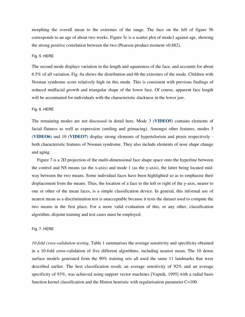
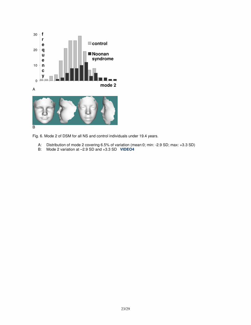
The second mode displays variation in the length and squareness of the face, and accounts for about

6.5% of all variation. Fig. 6a shows the distribution and 6b the extremes of the mode. Children with

Noonan syndrome score relatively high on this mode. This is consistent with previous findings of

reduced midfacial growth and triangular shape of the lower face. Of course, apparent face length

will be accentuated for individuals with the characteristic slackness in the lower jaw.

Fig. 6. HERE

The remaining modes are not discussed in detail here. Mode 3 (VIDEO5) contains elements of

facial flatness as well as expression (smiling and grimacing). Amongst other features, modes 5

(VIDEO6) and 10 (VIDEO7) display strong elements of hypertelorism and ptosis respectively -

both characteristic features of Noonan syndrome. They also include elements of nose shape change

and aging.

Figure 7 is a 2D projection of the multi-dimensional face shape space onto the hyperline between

the control and NS means (as the x-axis) and mode 1 (as the y-axis), the latter being located mid-

way between the two means. Some individual faces have been highlighted so as to emphasise their

displacement from the means. Thus, the location of a face to the left or right of the y-axis, nearer to

one or other of the mean faces, is a simple classification device. In general, this informal use of

nearest mean as a discrimination test is unacceptable because it tests the dataset used to compute the

two means in the first place. For a more valid evaluation of this, or any other, classification

algorithm, disjoint training and test cases must be employed.

Fig. 7. HERE

10-fold cross-validation testing. Table 1 summarises the average sensitivity and specificity obtained

in a 10-fold cross-validation of five different algorithms, including nearest mean. The 10 dense

surface models generated from the 90% training sets all used the same 11 landmarks that were

described earlier. The best classification result, an average sensitivity of 92% and an average

specificity of 93%, was achieved using support vector machines [Vapnik, 1995] with a radial basis

function kernel classification and the Hinton heuristic with regularisation parameter C=100.

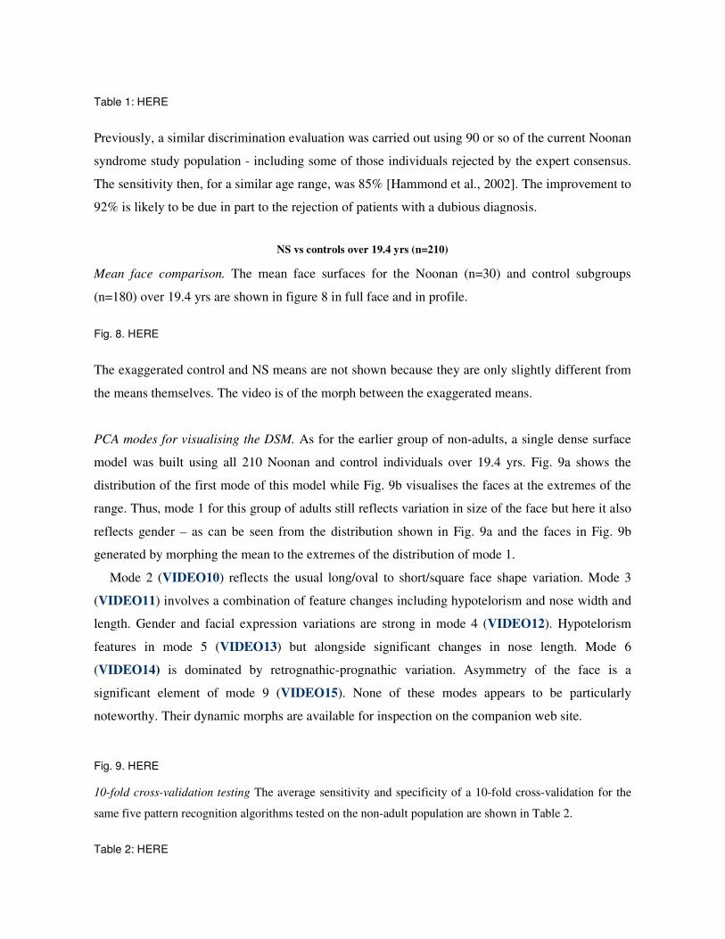
Table 1: HERE

Previously, a similar discrimination evaluation was carried out using 90 or so of the current Noonan

syndrome study population - including some of those individuals rejected by the expert consensus.

The sensitivity then, for a similar age range, was 85% [Hammond et al., 2002]. The improvement to

92% is likely to be due in part to the rejection of patients with a dubious diagnosis.

NS vs controls over 19.4 yrs (n=210)

Mean face comparison. The mean face surfaces for the Noonan (n=30) and control subgroups

(n=180) over 19.4 yrs are shown in figure 8 in full face and in profile.

Fig. 8. HERE

The exaggerated control and NS means are not shown because they are only slightly different from

the means themselves. The video is of the morph between the exaggerated means.

PCA modes for visualising the DSM. As for the earlier group of non-adults, a single dense surface

model was built using all 210 Noonan and control individuals over 19.4 yrs. Fig. 9a shows the

distribution of the first mode of this model while Fig. 9b visualises the faces at the extremes of the

range. Thus, mode 1 for this group of adults still reflects variation in size of the face but here it also

reflects gender – as can be seen from the distribution shown in Fig. 9a and the faces in Fig. 9b

generated by morphing the mean to the extremes of the distribution of mode 1.

Mode 2 (VIDEO10) reflects the usual long/oval to short/square face shape variation. Mode 3

(VIDEO11) involves a combination of feature changes including hypotelorism and nose width and

length. Gender and facial expression variations are strong in mode 4 (VIDEO12). Hypotelorism

features in mode 5 (VIDEO13) but alongside significant changes in nose length. Mode 6

(VIDEO14) is dominated by retrognathic-prognathic variation. Asymmetry of the face is a

significant element of mode 9 (VIDEO15). None of these modes appears to be particularly

noteworthy. Their dynamic morphs are available for inspection on the companion web site.

Fig. 9. HERE 10-fold cross-validation testing The average sensitivity and specificity of a 10-fold cross-validation for the

same five pattern recognition algorithms tested on the non-adult population are shown in Table 2.

Table 2: HERE

By comparison with the non-adult group, discrimination between individuals with Noonan

syndrome and controls in the adult group is considerably less successful. This is consistent with the

previously cited diminution in adulthood of characteristic facial differences in Noonan syndrome.

NS vs controls without age restriction (n= 430)

The comparison of means and the visualisation of modes is omitted here as they are similar to those

of the previous two sections. Instead, we simply give the results of the 10-fold cross-validation for

the same five pattern recognition algorithms in Table 3 below.

Table 3: HERE

These results, generally intermediate between those for the separate child and adult groups, are

consistent with diminishing differences in facial morphology during the maturing of individuals

with Noonan syndrome.

RESULTS: VCFS vs CONTROLS

VCFS vs controls between 3 and 17 yrs (n=190)

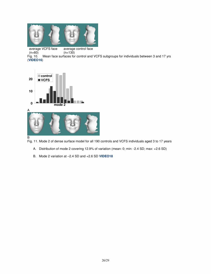
Mean faces The mean face surfaces for the VCFS (n=60) and control subgroups (n=130) between 3

and 17 years of age are shown in figure 11 in full face and in profile.

Fig. 10. HERE

The exaggerated morphs of the overall mean along the mean hyperline are only marginally different

from the means so their visualisation is not included here but on the companion web site.

Modes for visualising the DSM A dense surface model was generated for the combined VCFS and

control subgroups. The first mode of this model reflects the usual size of face variation (VIDEO17)

and accounts for 60.9% of shape variation. The second mode, covering 12.9% of shape variation,

reflects VCFS characteristics such as the longer nose, narrow nasal base and somewhat tubular

shape (Fig. 11), but also some facial expression.

Fig. 11. HERE

Figure 12 illustrates the same 2D projection of the face-shape space using a mean hyperline vs

mode 1 scatter plot as shown previously for Noonan syndrome. Once again, such within training set

testing of the nearest mean algorithm gives excellent discrimination between the two subgroups,

with just five faces misclassified.

Fig. 12: HERE

10-fold cross-validation The results of the unseen discrimination testing in Table 4 are not as good

as those for the Noonan syndrome-control comparison for a similar age range.

Table 4: HERE

They emphasise the obvious fact that individuals with VCFS have more subtle facial differences

from controls than is the case in Noonan syndrome. Moreover, the classification may also be

impaired by the fact that all but a handful of the VCFS 3D scans were captured with the older

scanner at a poorer resolution. Therefore, more subtle facial features may not be modelled well.

RESULTS: VCFS vs NS

VCFS vs NS between 2 and 20 yrs (n=120)

Exaggerated means The means and exaggerated morph along the mean hyperline are not illustrated

statically since they are very similar to images already shown in Figs. 3, 4 and 10. The dynamic

variation gives an excellent visualisation of the overall difference in facial morphology between NS

and VCFS. VIDEO19

PCA modes for visualising the DSM A dense surface model was generated to visualise the PCA

modes for the combined VCFS and NS subgroups. The first two modes of this model capture the

usual face size and shape variations. Modes 3 and 4, shown in Fig. 13 and scatter plotted in Fig. 14,

undergo the greatest change during the morph along the mean hyperline. Fig. 13. HERE

Fig. 14. HERE

Mode 3 emphasises differences in head width as well as mandible size and shape. Mode 4 strongly

reflects eye separation as well as width of both nasal bridge and nasal base. The nasal shape

differences are very noticeable, as would be expected with these two syndromes.

10-fold cross-validation The results of the unseen discrimination testing are shown in Table 5.

Table 5: HERE

These results are generally better than for the syndrome groups vs control discrimination tests. This

is due in part to the more even balancing of the training and test sets and suggests that in future a

more thorough investigation should be made of the interactions between training-test set balancing,

accuracy of face synthesis and discriminating ability.

DISCUSSION

In this study, we found that a novel method of 3D analysis demonstrates high levels of sensitivity

(88%) and specificity (94%) in discriminating between controls and individuals previously

diagnosed with Noonan syndrome and vetted visually by a further panel of four experienced clinical

geneticists. In addition, we found high levels of sensitivity (83%) and specificity (92%) in

discriminating between individuals with VCFS (diagnosed by fluorescence in situ hybridisation)

and controls. We suggest that this novel technique may assist the clinical geneticist in making a

diagnosis in individuals who present with complex or atypical facial features.

As the molecular defect in Noonan syndrome has yet to be characterised, the diagnosis is

generally made by experienced clinical geneticists. However, it is probable that a small minority of

patients, diagnosed with Noonan syndrome by clinical geneticists, do not in fact have Noonan

syndrome and are phenocopies. Thus, the high sensitivity and specificity of 3D facial analysis

reported in this study are potentially confounded by the possibility of diagnostic error. In view of

this, we also performed 3D image analysis in people with a known chromosome 22q11 deletion.

The high sensitivity and specificity we report in discriminating between people with VCFS and

controls demonstrates that diagnostic error is an unlikely explanation for the high discriminating

power of this technique in Noonan syndrome.

In comparison to the portable scanner (MU2), the older model (DSP400) does not capture both

ear surfaces consistently and captures far fewer surface points. As was previously explained, the

dense surface model involves computing an intersection of captured face surfaces, and so our

derived models may not include any ear surface at all depending on the particular images included

in the model. In Noonan syndrome, where low ear position is a characteristic trait, and in VCFS,

where ear shape can be dysmorphic, this is potentially damaging to any analysis.

Fig. 15. HERE

Fig. 15 and the associated dynamic morph demonstrate the huge improvement in the visualisation

when ears are included in the captured surface. Moreover, dense surface models generated from

such images are likely to discriminate with even greater success.

It is difficult to estimate the minimum number of 3D images needed before a dense surface

model supports useful visualisations or discrimination. Further testing is required before firm

conclusions can be drawn.

CONCLUSIONS

The still and dynamic images included here and on the accompanying website demonstrate that

dense surface models can generate striking and informative visualisations of facial morphology in

three dimensions. Any benefit they may provide in the training of clinical geneticists is yet to be

evaluated.

Dense surface models when combined with state of the art pattern recognition algorithms

achieve impressive results in discriminating between controls and individuals with a particular

syndrome, as well as between individuals with different syndromes – at least for the two syndromes

covered. It is also encouraging that the results presented here were obtained using 3D meshes of

different resolutions and quite varied coverage, often missing anatomical features important in

facial dysmorphology.

As was remarked earlier, the larger the number of examples included in a dense surface model

the greater the accuracy of the synthesis of each face using the associated modes. The rarity of some

syndromes will limit the available dataset and imbalance the mix of controls and individuals with a

particular syndrome. Inevitably, this will reduce the discrimination accuracy. Therefore, it is

important that image capture is undertaken on an international basis, with sharing of data once

appropriate ethical approval and patient or parent consent is obtained.

Our collection of 3D face scans also includes individuals with Angelman, Rett, Rubinstein-

Taybi, Smith-Magenis and Williams syndromes. Having demonstrated that dense surface models

show promise in delineating and discriminating face shape associated with Noonan and Velo-

cardio-facial syndromes, separate studies of the comparative 3D facial morphologies of individuals

with these other syndromes have begun. As the data gathering for these becomes more

internationally widespread, it will also become possible to address the issue of ethnic variation in

facial morphology. Similar unavoidable confounding factors when considering facial morphology,

of course, are gender, age and familial likeness. Before these can begin to be addressed, much more

data needs to be gathered.

ACKNOWLEDGEMENTS The authors are extremely grateful to the patients, families and volunteers who took part in this

study. Birth Defects Foundation (BDF) provided generous funding for the DSP400 scanner (Grant

Ref:2000/27) and the Wellcome Trust provided a small travel grant (Grant Ref:TG02). BDF also

provided opportunities for scanning attendees at their Noonan syndrome family meetings in UK.

We also thank PPP Healthcare Medical Trust whose funding supported the involvement of children

with VCFS (Grant Ref: 1206/188) and the 22q11 (UK) Support Group who kindly helped with

recruitment. The St Albans Clinic in Highgate, London clinic and attending parents kindly

consented for their children to be included as controls in the study. Dr Henry Potts and Dr Caroline

Deys are thanked for helping to arrange attendance at the clinic. Professor Bernard Buxton (Dept. of

Computer Science, UCL) was generous with his advice during discussions of the data analysis.

REFERENCES

Allanson JE. 1997. Objective Techniques for Craniofacial Assessment: What Are the Choices? Am J Med Genet 70:1-5. Allanson JE, Cole TRP. 1996. Sotos syndrome: evolution of the facial phenotype subjective and objective assessment. Am J Med Gen 65:13-20. Allanson JE, Hennekam RCM. 1997. Rubinstein-Taybi Syndrome: objective evaluation of craniofacial structure. Am J Med Gen 71:414-419. Allanson JE, Hall JG, Hughes HE, Preus M, Witt RD. 1985. Noonan Syndrome: The Changing Phenotype. Am J Med Genet 21:507-514. Allanson JE, O’Hara, Farkas, Nair RC. 1993. Anthropometric craniofacial pattern profiles in Down syndrome. Am J Med Gen 47:748-752. Arridge S, Moss JP, Linney AD, James DR. 1985. Three dimensional digitisation of the face and skull. J Maxillofac Surg 13(3):136-143. Astley SJ, Clarren SK. 1996. A case definition and photographic screening tool for facial phenotype of fetal alcohol syndrome. The Journal of Pediatrics 129(1):33-41. Ayoub A, Siebert P, Moos K, Wray D, Urquhart X, Niblett T. 1998. A vision-based thee-dimensional capture system for maxillofacial assessment and surgical planning. Brit J Oral and Maxillofac Surg 36:353-357.

BDF (Birth Defects Foundation). http://www.birthdefects.co.uk Chang C-C, Lin C-J. 2001. LIBSVM : a library for support vector machines. http://www.csie.ntu.edu.tw/~cjlin/libsvm CLEM: http://www.spss.com/spssbi/clementine/ Bookstein FL. 1997. Shape and the information in medical images: a decade of the morphometric synthesis. Comput Vis Image Process 33:33-80. Braaten O. 1996. Artificial Intelligence in Pediatrics: important clinical signs in newborn syndromes. Comput Biomed Res 29: 153-161. Dryden IL, Mardia KV. 1998. Statistical Shape Analysis. Chichester: John Wiley and Sons. Evans CD. 1995. A case-based assistant for diagnosis and analyis of dysmorphic syndromes Med Inf 20:121-131. Evans CD, Winter RM. 1995. MD Computing 12(2):127-136. Gower JC. 1975. Generalized proscrustes analysis. Psychometrika 40:33-51. Guyot L, Dubuc M, Pujol J, Dutout O, Philip N. 2001. Craniofacial analysis in patients with 22q11 microdeletion. Am J Med Gen 100:1-8. Hammond P, Hutton TJ, Nelson-Moon ZL, Hunt N, Madgwick AJA. 2001a. Classifying Vertical Facial Deformity using Supervised and Unsupervised Learning. Meth Inf Med 40: 365-372. Hammond P, Hutton TJ, Patton MA, Allanson JE. 2001b. Delineation and Visualisation of Congenital Abnormality using 3D Facial Images. In: Bellazzi R., Zupan B., Liu X. (Eds.), Proceedings of the Workshop Intelligent Data Analysis in Medicine and Pharmacology, IDAMAP2001 at MedInfo2001, London, UK. Hammond P, Hutton T, Allanson JA, Shaw A, Patton MA. 2002. 3D Digital Stereo Photogrammetric Analysis of Face Shape in Noonan Syndrome. J Med Genet 39: Supplement 1, S35. Hanihara T. 2000. Frontal and facial flatness of major human populations. Am J Phys Anthropol 111:105-134. Hennessy RJ, Stringer CB. 2002. Geometric Morphometric Study of the Regional Variation of Modern Human Craniofacial Form. Am J Phys Anthropol 117:37-48. Horsthemke B, Wieczorek D, Loos HS, von der Malsburg C. 2002. Computer-based recognition of syndromic faces. Proc Am Soc Hum Gen 2002, Baltimore, USA. Hovis CL, Butler MG. 1997. Photoanthropometric study of craniofacial traits in individuals with Williams syndrome. Clin Genet 51(6): 379-387. Hutton TJ, Buxton BF, Hammond P. 2001. Dense surface point distribution models of the face. Proc IEEE Workshop on Mathematical Methods in Biomedical Image Analysis, Kauai, Hawaii: 153-160. Hutton TJ, Buxton BF, Hammond P, Potts HWW. 2003. Estimating Average Growth Trajectories in Shape-Space using Kernel Smoothing. IEEE Trans Med Imaging (in press).

Kendall DG. 1984. Shape-Manifolds, Procrustean metrics, and complex projective spaces. Bull Lond Math Soc 16:81-121. Mass E, Belostoky L. 1993. Craniofacial morphology of children with Williams syndrome. Clef Palate Craniofac J 30(3): 343-349. Meintjes EM, Douglas TS, Martinez F, Vaughan CL, Adams LP, StekhovenA, Viljoen D. 2002. A stereo-photogrammetric method to measure the facial dysmorphology of children in the diagnosis of fetal alcohol syndrome. Med Eng & Phys 24: 683-689. Minugh-Purvis N, Kirschner RE, Slemp AE, McDonald-McGinn DM, Zackai EH, LaRossa D, Emanuel BS. 2002. Craniofacial dysmorphology in 22q11.2 deletion syndrome: an anthropometric analysis. Proc DELETION 22q11.2 Third International Meeting, Italy. O’Higgins P. 2000. The study of morphological variation in the human fossil record: biology, landmarks and geometry. J Anat 197:103-120. O’Higgins P, Jones N. 1998. Facial growth in Cercocebus torquatus: an application of three-dimensional geometric morphometric techniques to the study of morphological variation. J Anat 193: 251-272. Pelz J, Arendt V, Kunze J. 1998. Computer assisted diagnosis of malformation syndromes: an evaluation of three datanases (LDDB, POSSUM, SYNDROC) Am J Med Genet 63(1):257-267. Sampson PD, Streissguth A, Bookstein FL, Barr H. 2000. On categorizations in analyses of alcohol teratogenesis. Environmental Health Perspectives 108 (3):421-428. Scutt LE, Chow EWC, Weksberg R, Honer WG, Bassett AS. 2001. Patterns of Dysmorphic Features in Schizophrenia. Am J Med Gen (Neuropsychiatric Genetics) 105:713-723. Sharland M, Morgan M, Patton MA. 1993. Photoanthropometric Study of Facial Growth in Noonan Syndrome. Am J Med Genet 45:430-436. Shaw A, van der Burgt I, Brunner HG, Noordam K, Kalidas K, Crosby AH, Ion A, Jeffrey S, Patton MA, Tartaglia M, Gelb BD. 2002. Genotype and Phenotype analysis of 127 patients with Noonan Syndrome. Proc ESHG, Strasbourg. Sokol RJ, Chik L, Martier SS, Salari V. 1991. Morphometry of the neonatal fetal alcohol syndrome face from ‘snapshots’. Alcohol Suppl 1:531-534. Stengel-Rutkowski S, Schimanek P, Wernheimer A. 1984. Anthropometric definitions of dysmorphic facial signs. Hum Genet 67:272-295. Tartaglia M, Mehler EL, Goldberg R, Zampino G, Brunner HG, Kremer H, van der Burgt I, Crosby AH, Ion A, Jeffrey S, Kalidas K, Patton MA, Kucherlapati RS, Gelb BD. 2001. Mutations in PTPN11, encoding the protein tyrosine phosphatase SHP-2, cause Noonan syndrome. Nat Gen 29: 465-467. TNSSG. http://www.noonansyndrome.org/home.html Vapnik V. 1995. The nature of statistical learning theory. New York: Springer. VCFSEF. http://www.vcfsef.org/ Winter RM. 1996. What’s in a face? Nat Gen 12: 124-129.

Winter RM, Clark RD, Ashley K, Gibbs G. 1988. A combinatorial method for grouping cases with multiple malformations. J Med Genet 25 (2):118-121.

TABLES

Nearest Mean

Decision Trees

Neural Networks

Logistic Regression

Support Vector

Machines Sens Spec Sens Spec Sens Spec Sens Spec Sens Spec

88%

86%

60%

83%

83%

94%

83%

93%

92%

93%

Table 1: average sensitivity and specificity of cross validation (age<19.4 yrs; NS = 60; control = 160)

Nearest Mean

Decision Trees

Neural Networks

Logistic Regression

Support Vector

Machines Sens Spec Sens Spec Sens Spec Sens Spec Sens Spec

80%

94%

20%

92%

60%

96%

60%

93%

83%

94%

Table 2: average sensitivity and specificity of cross validation (age>=19.4 yrs; NS = 30; control = 180)

Nearest Mean

Decision Trees

Neural Networks

Logistic Regression

Support Vector

Machines Sens Spec Sens Spec Sens Spec Sens Spec Sens Spec

81%

82%

44%

85%

68%

96%

84%

93%

88%

94%

Table 3: average sensitivity and specificity of cross validation (NS = 90; control = 340)

Nearest Mean

Decision Trees

Neural Networks

Logistic Regression

Support Vector

Machines Sens Spec Sens Spec Sens Spec Sens Spec Sens Spec

82%

85%

58%

81%

57%

97%

75%

90%

83%

92%

Table 4: average sensitivity and specificity of cross validation (VCFS = 60; control = 130)

Nearest Mean

Decision Trees

Neural Networks

Logistic Regression

Support Vector

Machines Sens Spec Sens Spec Sens Spec Sens Spec Sens Spec

85%

90%

86%

71%

91%

87%

93%

89%

95%

95%

Table 5: average sensitivity and specificity of cross validation (using 60 NS as –ve and 60 VCFS as +ve)

21/29

FIGURES

Fig. 1. Multiple cameras of DSP400 3D face scanner

A B C Fig. 2. 3D Face image capture A: random speckle pattern projected onto face showing one of four views/patches used to generate surface

of the face; B: surface of face computed from 4 patches; C: 11 landmarks typically located on each 3D image and used to build the dense surface models

average NS face

(n=60) average control face

(n=160)Fig. 3. Mean face surfaces for control and Noonan syndrome subgroups for individuals under 19.4 years VIDEO1

Noonan extreme of

morph Control extreme of

morph Fig. 4. Morph of overall mean along the mean hyperline VIDEO2

22/29

0

10

20

30

mode 1

frequency

control

Noonan syndrome

A

B

-4

-3

-2

-1

0

1

2

3

0 5 10 15 20age

mode 1

control

Noonan syndrome

C Fig. 5. Mode 1 of DSM for all NS and control individuals under 19.4 years.

A. distribution of mode 1 covering 73.1% of variation (mean: 0; min: -3.5 SD; max: +2.3 SD); B. Mode 1 variation at –3.5 and 2.3 SD; VIDEO3 C. Scatter plot of mode 1 against age

23/29

0

10

20

30

mode 2

frequency

control

Noonan syndrome

A

B Fig. 6. Mode 2 of DSM for all NS and control individuals under 19.4 years.

A: Distribution of mode 2 covering 6.5% of variation (mean:0; min: -2.9 SD; max: +3.3 SD) B: Mode 2 variation at –2.9 SD and +3.3 SD VIDEO4

24/29

-4

-3

-2

-1

0

1

2

3

mean hyperline

mode 1

Noonan syndromecontrol

Fig. 7. Scatter plot of mean hyperline against mode 2 for non-adult controls (n=160) and individuals with Noonan syndrome (n=60) The labelled faces are misclassified according to the nearest mean discrimination test. Faces D and E are of very young babies and given the small number of such children in the database, their misclassification is not surprising. Face C is just closer to the NS mean in this model. Faces A and B are misclassified as controls, but it happens that some of their features are quite uncharacteristic of Noonan syndrome. For ethical reasons, the faces of these individuals are not shown.

E

D

C B

A

NS mean

control mean

25/29

average NS (n=30) average control

(n=180) Fig. 8. Mean face surfaces for control and Noonan syndrome individuals over 19.4 yrs (VIDEO8)

0

10

20

30

mode 1

male female

A

B Fig. 9. Mode 1 of DSM for all 210 controls and individuals with Noonan syndrome over 19.4 years of age A: distribution (mean: 0; min –2.9 SD; max:2.1 SD) B: Mode 1 at –2.9 SD and 2.1 SD (VIDEO9)

26/29

average VCFS face (n=60)

average control face (n=130)

Fig. 10. Mean face surfaces for control and VCFS subgroups for individuals between 3 and 17 yrs (VIDEO16)

0

10

20

mode 2

controlVCFS

A

B Fig. 11. Mode 2 of dense surface model for all 190 controls and VCFS individuals aged 3 to 17 years

A. Distribution of mode 2 covering 12.9% of variation (mean: 0; min: -2.4 SD; max: +2.6 SD) B. Mode 2 variation at –2.4 SD and +2.6 SD VIDEO18

27/29

Fig. 12: Scatter plot of mean hyperline (x-axis) against mode 1 (y-axis) for controls (n=130) and individuals with VCFS (n=60). The five faces labelled A to E are misclassified according to the nearest mean discrimination test. As with figure 7, individual faces are not shown. The images included illustrate the extremes for each of the axes.

-3

-2

-1

0

1

2

3

mean hyperline

mode 1

VCFScontrol

A

B

C

D

E

VCFS mean control mean

28/29

A

B Fig. 13. Modes 3 and 4 of DSM for NS (n=60) and VCFS (n=60) individuals aged 2 to 20 years A: Mode 3 at –3.3 and 2.2 SD VIDEO20 B: Mode 4 at –2.1 and 3.1 SD VIDEO21

-2.5

-1.5

-0.5

0.5

1.5

2.5

3.5

-3.5 -2.5 -1.5 -0.5 0.5 1.5 2.5 3.5 mode 3

mode4

NS VCFS

Fig. 14. Scatter plot of modes 3 and 4 of DSM for NS (n=60) and VCFS (n=60) individuals aged 2 to 20 years illustrating their partial discriminating ability

Fig. 15. Extreme faces on mean hyperline for NS versus control using a subset of images with good ear coverage (n=106) VIDEO22

29/29