3d modelling of turbulence in a mag- netically confined ... · 3d modelling of turbulence in a...
TRANSCRIPT

U N I V E R S I T Y O F C O P E N H A G E N
F A C U L T Y O F S C I E N C E
3D Modelling of Turbulence in a Mag-netically Confined Toroidal Plasma
Master Thesis
Aske Anguasak Busk Olsen
Niels Bohr Institute
Supervisor: Peter Ditlevsen, Jens Juul Rasmussen (DTU) and Jens Madsen (DTU)
Submitted: November 29, 2016

U N I V E R S I T Y O F
C O P E N H A G E N
Faculty: Science
Institute: Niels Bohr Institute
Author: Aske Anguasak Busk Olsen
Email: [email protected]
Title and Subtitle: 3D Modelling of Turbulence in a Magnetically ConfinedToroidal Plasma- Master Thesis
Supervisor: Peter Ditlevsen, Jens Juul Rasmussen (DTU) and JensMadsen (DTU)
Handed in: November 29, 2016
Defended: 12/12-2016
Name
Signature
Date

Acknowledgements
I would like to thank my internal supervisor Peter Ditlevsen, and my externalsupervisors Jens Juul Rasmussen and Jens Madsen for guidance and alwaysbeing helpful.
I want to dedicate a special thanks to the BOUT++ expert, of the PPFEgroup at DTU, Michael Løiten Magnussen for always being helpful and an-swering a lot of questions regarding the BOUT++ platform.
Finally I send a special thanks to my brother, Jeppe Miki Busk Olsen,for igniting my interest in plasma physics.


Abstract
Nuclear fusion has been proposed as an alternative clean energy source. Inorder to have a deep understanding of the dynamic properties of a fusionplasma an accurate model is needed. Most investigations of fusion plasmashave been done using two dimensional models, even though a realistic modelinvolves dynamics in three dimensions.
This thesis sets out to create a coordinate system aligned with the mag-netic field in order to create a realistic model in three dimensions whilsthaving a coarse resolution in the direction of the magnetic field.
Using the model created, an investigation of the Hasegawa-Wakataniequations was done. Three different cases were investigated using three dif-ferent values of magnetic shear.
The simulations showed a dependence on the magnetic shear for the sta-bility of the system which is in accordance theory. The field-aligned coor-dinate system created in this thesis shows promising results as the platformfor future simulations in three dimensions.


Contents
1 Introduction 11.1 Motivation . . . . . . . . . . . . . . . . . . . . . . . . . . . . . 11.2 Thermonuclear Fusion . . . . . . . . . . . . . . . . . . . . . . 21.3 The Tokamak . . . . . . . . . . . . . . . . . . . . . . . . . . . 7
2 The Two Fluid Equations 112.1 The Vlasov Equation . . . . . . . . . . . . . . . . . . . . . . . 11
2.1.1 Moments and collisions in the Vlasov equation . . . . . 132.2 The closure problem . . . . . . . . . . . . . . . . . . . . . . . 212.3 Drift Equations . . . . . . . . . . . . . . . . . . . . . . . . . . 22
3 Differential Geometry 253.1 Contra- and Covariant vectors . . . . . . . . . . . . . . . . . . 253.2 The Metric and the Jacobian . . . . . . . . . . . . . . . . . . 283.3 Differential operators in curvilinear geometry . . . . . . . . . . 30
4 Field aligned coordinates 334.1 The shape of the Magnetic Field . . . . . . . . . . . . . . . . . 33
4.1.1 MHD equilibrium . . . . . . . . . . . . . . . . . . . . . 354.2 Modified Hamada coordinates . . . . . . . . . . . . . . . . . . 384.3 Field-Aligned Hamada Coordinates . . . . . . . . . . . . . . . 414.4 The Circle Equilibrium Model . . . . . . . . . . . . . . . . . . 43
4.4.1 The Contravariant Hamada Metric . . . . . . . . . . . 464.4.2 The Contravariant Field-Aligned Hamada Metric . . . 48
5 The Hasegawa-Wakatani Equations 515.1 Assumptions . . . . . . . . . . . . . . . . . . . . . . . . . . . . 515.2 The Electron Fluid . . . . . . . . . . . . . . . . . . . . . . . . 54

CONTENTS
5.3 The Ion Fluid . . . . . . . . . . . . . . . . . . . . . . . . . . . 565.4 Normalizing the Hasegawa-Wakatani equations . . . . . . . . . 56
6 Simulations of the Hasegawa-Wakatani System 616.1 The Metric . . . . . . . . . . . . . . . . . . . . . . . . . . . . 616.2 Simple Diffusion . . . . . . . . . . . . . . . . . . . . . . . . . . 65
6.2.1 Cross-section and Interpolation . . . . . . . . . . . . . 656.3 The Dispersion Relation and Unstable Modes . . . . . . . . . 706.4 Numerical Simulations of The Hasegawa-Wakatani Model . . . 76
6.4.1 Numerical Simulations With Magnetic Shear . . . . . . 76
7 Conclusion 937.1 Future Prospects . . . . . . . . . . . . . . . . . . . . . . . . . 94
A Toroidal Metric Coefficients 95
B Useful Vector Identities 99

Chapter 1
Introduction
1.1 Motivation
Since the beginning of the industrial revolution there has been an almostexponential growth in worldwide energy consumption, which has lead toan increase in emission of greenhouse gasses. Studies have shown a linkbetween an increase of greenhouse gasses in the atmosphere and an increasein the global temperature. [1] The higher temperatures on earth can lead tomore extreme weather conditions and more non-nutritious land. So unlesssomething is done to stop the emission of greenhouse gasses the world standsbefore a potential environmental catastrophe.
Many steps have been, and are currently being taken, in order to re-duce the emission of greenhouse gasses. Various forms of sustainable energysources have been investigated. However most of the sustainable sources ofenergy have some problematic traits.
Wind energy works fine in countries such as Denmark, a country thatis windy at almost all times. However even though wind energy might attimes meet the needs of a country like Denmark, it is highly unreliable dueto the chaotic nature of wind systems. At times where the windmills generateexcessive power there is currently no efficient way of storing the energy, sincemost batteries are quite inefficient. Furthermore batteries consists of liquidsthat are harmful to the environment. Another issue with windmills is thatthey are only usable in windy countries. This means that windmills may bepart of the solution for having 100% sustainable energy, but not the onlysolution.
1

2 CHAPTER 1. INTRODUCTION
A similar problem arises with hydroelectric plants, it is great in countrieslike Norway, a country with a lot of mountains that are necesarry in orderfor hydroelectric plants to work, however countries with no mountains cannot rely on hydroelectric plants as the main energy source.
Solar cells rely on sunlight, and are, as windmills, unreliable. Furthermorecurrent solar cells are fragile and easily broken.
In conclusion solar-, wind- and hydroelectric energy can not stand aloneas environmentally sustainable energy sources, which means there is a needfor other sustainable energy sources. Another source of energy that couldpotentially cover the global need is nuclear energy by fission. However aproblem arises with storage of the radioactive waste, where the waste has ahalf-life of up to ∼ 200000 years [2]. Although discussion can be made asto whether or not the storage of the waste is an unsolvable problem there isstill opposition among the general population towards nuclear fission.
This leads to one final solution to the energy crisis, which is nuclearfusion. There is radioactive waste from fusion reactions, however the amountof radioactive waste is not large, and the half-life of the waste is short (∼12years [3]) and the waste can be confined within the power plant, makingtransportation unnecessary. Working fusion reactors might be the solutionto obtaining energy production based solely on sustainable energy due to theabundance on earth of the fuels used in a nuclear power plant.
1.2 Thermonuclear Fusion
A plasma is a gas consisting of ionized particles. The reaction of interest in aplasma used for fusion power is the one between tritium (3H) and deuterium(2H) [4]. Tritium can be obtained by splitting lithium, a common metal,and deuterium is found in water(∼ 0.0156% of the water [5]). The fusionbetween tritium and deuterium gives a high energy output [4], and as seenin figure 1.1, which is a plot of the cross sections of three different reactionsas a function of temperature, it has the highest cross section between 10 and100 keV deuteron energy of the three reactions shown (the cross section is ameasure of the probability of the two fusing).
The reaction of interest is thus
21H +3
1 H→42 He + n (1.1)

1.2. THERMONUCLEAR FUSION 3
Figure 1.1: The cross section as a function of deuteron energy [4].
The system must conserve energy and momentum, allowing us to calculatethe energy freed in the fusion process. The sum of the rest energy of tritiumand deuterium can be subtracted from the sum of the rest energy of heliumand a neutron. We know that the excessive energy must be stored in themomentum of the neutron and the momentum of the helium core. The restenergy is given by Einsteins equation [2]
Erest = mc2 (1.2)
The mass of deuterium is 2.01410178 u [2], the mass of tritium is 3.0160492u, the mass of helium is 4.002602 u and the mass of the neutron is 1.008664u. The energy freed is thus
2.01410178u + 3.0160492u− (4.002602u + 1.008664u) = 0.01888498u
One atomic mass unit is equivalent to 931.494 MeVc
[2] and we have
0.01888498 · 931.494MeV = 17.6MeV
4 CHAPTER 1. INTRODUCTION
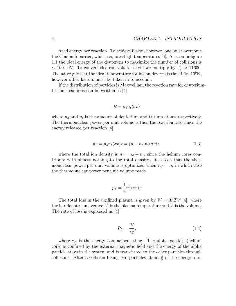
freed energy per reaction. To achieve fusion, however, one must overcomethe Coulomb barrier, which requires high temperatures [6]. As seen in figure1.1 the ideal energy of the deuterons to maximize the number of collisions is∼ 100 keV. To convert electron volt to kelvin we multiply by e
kB≈ 11600.
The naive guess at the ideal temperature for fusion devices is thus 1.16·109K,however other factors must be taken in to account.
If the distribution of particles is Maxwellian, the reaction rate for deuterium-tritium reactions can be written as [4]
R = ndnt〈σv〉
where nd and nt is the amount of deuterium and tritium atoms respectively.The thermonuclear power per unit volume is then the reaction rate times theenergy released per reaction [4]
pT = ndnt〈σv〉ε = (n− nt)nt〈σv〉ε, (1.3)
where the total ion density is n = nd + nt, since the helium cores con-tribute with almost nothing to the total density. It is seen that the ther-monuclear power per unit volume is optimized when nd = nt in which casethe thermonuclear power per unit volume reads
pT =1
4n2〈σv〉ε
The total loss in the confined plasma is given by W = 3nTV [4], wherethe bar denotes an average, T is the plasma temperature and V is the volume.The rate of loss is expressed as [4]
PL =W
τE, (1.4)
where τE is the energy confinement time. The alpha particle (heliumcore) is confined by the external magnetic field and the energy of the alphaparticle stays in the system and is transferred to the other particles throughcollisions. After a collision fusing two particles about 4
5of the energy is in

1.2. THERMONUCLEAR FUSION 5
the neutron and the rest is in the alpha particle [4]. In order to have as muchenergy stay in the system as is lost, we must have
PH + Pα = PL,
where PH is an external power source, and Pα is the heating causedby the α-particles. The total α-particle heating can also be expressed as14n2〈σv〉εαV [4], where the bar denotes an average, and εα is the energy
carried by the α-particles.It is possible to have all required heating of the plasma, come from the
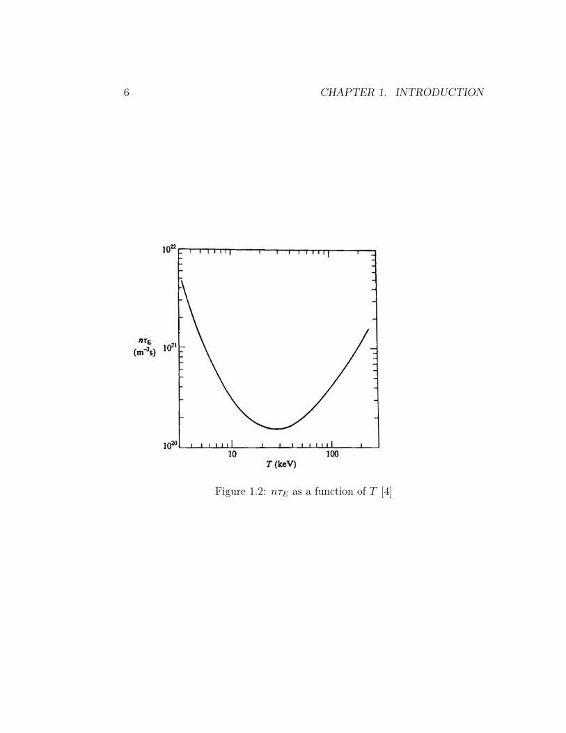
α-particle heating. When this is achieved it is called ignition. The ignitioncriteria is thus that Pα > PL or
nτE ≥12
〈σv〉T
εα, (1.5)
where the bars have been omitted for convenience. The right hand sideis only a function of temperature and a graph of nτE as a function of T canbe seen in figure 1.2. As seen on the graph the minimum required nτE forignition occurs at T ∼ 20keV or at approximately 200 million degrees kelvin.
Since ignition is required for fusion devices as an energy source, the op-timal temperature for a fusion device is at 20 keV. However no known solidmaterial can withstand such temperatures, and another way of confining theplasma is needed. Luckily, a plasma consists of charged particles and can thusbe confined by an external magnetic field. The two currently most promisingdevices, are the tokamak and the stellarator, where the focus in this thesisis on the tokamak.
6 CHAPTER 1. INTRODUCTION
Figure 1.2: nτE as a function of T [4]

1.3. THE TOKAMAK 7
1.3 The Tokamak
The tokamak is a device for confining a plasma by the use of an externalmagnetic field. It is torus-shaped with magnetic coils surrounding it. Inorder to create a magnetic field that confines the plasma, both magneticfields in the poloidal and toroidal directions are generated [4].
Figure 1.3 is a graphical illustration of a tokamak, showing the toroidal-and inner and outer poloidal coils, which result in twisted magnetic field linesin the plasma. The magnetic field of the tokamak is described in detail inchapter 4 and is a central part of understanding the dynamics of a magneti-cally confined plasma. The in depth handling of the subject is therefore leftfor the chapter. I will, however, give a brief introduction to the shape of themagnetic field.
The magnetic field can be expressed by a toroidal and poloidal part, witha toroidal field given by
Bt = I(ψ)∇φ,
where I is a function of the poloidal flux function, ψ, and φ is the toroidalangle, and the poloidal field given by
Bp = ∇φ×∇ψ. (1.6)
Usually when touching the subject of a fusion plasma the analysis iscentered around three different regions of the fusion plasma. The core region,where the magnetic field lines are closed, i.e. when the field lines will at somepoint close in on themselves, and form almost circular poloidal cross sections.The edge region that includes an X-point, which is the point at which themagnetic field lines go from closed to open. The X-point is sometimes calledthe separatrix. And finally a region of open field lines called the scrape oflayer (SOL). Figure 1.4 shows the poloidal cross section of a tokamak, wherethe described regions can be seen. This thesis focuses on the edge regionright before the X-point.
The shape of the magnetic field will be used to create a field-alignedcoordinate system, used for simulating the Hasegawa-Wakatani equations,a simplified fluid model describing the dynamics a fusion plasma, and willcreate a platform with the possibility of simulating more complex equationsin the future.

8 CHAPTER 1. INTRODUCTION
Figure 1.3: Graphical illustration of a tokamak [7].
Figure 1.4: Poloidal cross section of a tokamak [8].
1.3. THE TOKAMAK 9
The outline of this thesis is as follows:In chapter 2 a fluid description of fusion plasma dynamics is derived.Chapter 3 gives a short description of the differential geometry used in
this sectionIn chapter 4 a description of the shape of the magnetic field is described
followed by a derivation of a set of coordinates aligned with the magneticfield.
In chapter 5 the Hasegawa-Wakatani model in curvilinear geometry isderived, by using simplifying assumptions on the fluid equations derived inchapter 2.
Chapter 6 describes the results of simulations perfomed for the Hasegawa-Wakatani model found in chapter 5.
And finally in chapter 7 we have the conclusion.

10 CHAPTER 1. INTRODUCTION

Chapter 2
The Two Fluid Equations
1A plasma usually consists of at least two species of particles and it is there-fore convenient to describe a plasma in terms of these different species. Inprinciple if the momenta and positions of all particles in a plasma are knownat a given time, the behaviour of the plasma could be described exact. How-ever a fusion plasma usually consists of more than 1024 particles of differentspecies, making it impossible to simulate plasma properties using an indi-vidual particle model due to limited processing power, even if the initialmomenta and positions of all particles are known.
It is therefore convenient to model a plasma differently, and it turns outthat a plasma can be modelled as a fluid by using few assumptions.
2.1 The Vlasov Equation
In order to describe the evolution of a plasma we start by considering a pointin one-dimensional phase space, which can be represented by the distributionfunction f(x, v, t). Next, we examine a box in one-dimensional phase spaceof width dx and of height dv (see figure 2.1 [9]). Now the rate of changeof particles in the one dimensional box can be described. The particle fluxin the horizontal direction is given by f(x, v, t)v, where v = dx
dtand in the
vertical direction by f(x, v, t)a, where the acceleration a = dvdt
.The flux into the left side of the box is given by the flux at x times the
length of the side, so f(x, v, t)vdv, and into the right side at x + dx with
1This chapter is a continuation of material written by me for a project in plasmaphysics.
11

12 CHAPTER 2. THE TWO FLUID EQUATIONS
Figure 2.1: A box within phase-space having width dx and height dv. [9]
length dv it is given by −f(x+ dx, v, t)vdv.The flux into the bottom of the box at v with the length of the bottom
being dx is f(x, v, t)adx, and into the top it is −f(x, v + dv, t)adx.The total rate of change in the box will then be given by
∂f(x, v, t)
∂tdvdx = −f(x+ dx, v, t)vdv + f(x, v, t)vdv
−f(x, v + dv, t)adx+ f(x, v, t)adx (2.1)
Since we are in phase space v is independent of x, so all x operatorscommute with v and vice versa. Furthermore dividing by dvdx and using
limdx→0
f(x+ dx, v, t)v − f(x, v, t)v
dx= v
∂f(x, v, t)
∂x,
and
limdv→0
f(x, v + dv, t)a− f(x, v, t)a
dv=∂(af(x, v, t))
∂v,
we arrive at the one dimensional Vlasov equation.
∂f(x, v, t)
∂t+ v
∂f(x, v, t)
∂x+∂(af(x, v, t))
∂v= 0. (2.2)

2.1. THE VLASOV EQUATION 13
This can be generalized to three dimensions [9]
∂f(x,v, t)
∂t+ v
∂f(x,v, t)
∂x+∂(af(x,v, t))
∂v= 0.
The acceleration in the case of a plasma is given by the Lorentz force [9],
a =q
m(E + v×B). (2.3)
Since (v×B)i is perpendicular to vi we have
∂(v×B)i∂vi
= 0,
meaning that ∂∂v
and a commute. Using this, the Vlasov equation can berewritten to
∂f(x,v, t)
∂t+ v · ∂f(x,v, t)
∂x+ a · ∂f(x,v, t)
∂v= 0. (2.4)
2.1.1 Moments and collisions in the Vlasov equation
In the following section moments will be taken of the Vlasov equation to geta useful description of a two-fluid plasma. Taking moments is the procedureof multiplying f by powers of v and integrating it with respect to v [9]. Sincewe will be looking at the dynamics of different species, we denote f by itsspecie type σ as fσ. To get the particle density in configuration space, weintegrate the distribution function with respect to velocity in phase space,
n(x, t) =
∫fσ(x,v, t)dv. (2.5)
The mean velocity of the particles is given by
u =
∫vfσ(x,v, t)
n(x, t)dv. (2.6)

14 CHAPTER 2. THE TWO FLUID EQUATIONS
Figure 2.2: View of collisions in 1D phase space [9]
Collisions of two particles (nuclei and electrons) of different species changesthe speed of the two particles significantly, whilst remaining at approximatelythe same position. An illustration of a collision can be seen in figure 2, andas seen from the figure you can view collisions as an annihilation of the col-liding particles and the creation of two new [9]. The coupling of annihilationand creation rates constrains the form of the collision operator. Includingcollisions the Vlasov equation now takes the form:
∂fσ(x,v, t)
∂t+ v · ∂fσ(x,v, t)
∂x+ a · ∂fσ(x,v, t)
∂v=∑α
Cσα(fσ(x,v, t)) (2.7)
Where Cσα is the rate of change of fσ due to collisions between particlesof species σ with species α.
Constraints on the collision operator will help in the derivation of themoments of the Vlasov equation. The constraints on the collision operatorare:
Constraint 1 Conservation of particles. A collision will not change thenumber of particles at a specific location (unless of course there is fusion,but even in high reaction plasmas, collisions where the two particles fuse arenegligible on a large scale compared to other collisions).

2.1. THE VLASOV EQUATION 15
∫dvCσα(fσ) = 0 (2.8)
Constraint 2 Conservation of momentum. As in all other physical situ-ations momentum must be conserved.
∫dvmσvCσα(fσ) +
∫dvmαvCασ(fα) = 0 (2.9)
Constraint 3 Conservation of energy. As in all other isolated physicalsystems energy must be conserved.
∫dvmσv
2Cσα(fσ) +
∫dvmαv
2Cασ(fα) = 0 (2.10)
where v2 = v·v. With these constraints on the collision operator in mind,we are now able to take the first three moments of the Vlasov equation (0th,1st and 2nd). Taking the zeroth moment we have
∫ (∂fσ(x,v, t)
∂t+ v · ∂fσ(x,v, t)
∂x+ a · ∂fσ(x,v, t)
∂v
)dv =
∫dv∑α
Cσα(fσ(x,v, t)).
(2.11)
The derivatives of the first and second term of the left hand side bothcommute with the velocity integral, leaving us with an integral of the distri-bution function over all of velocity space. The right hand side gives zero dueto our constraints on the collision operator. Evaluating the integral of thethird term we have
∫V
dv∇v · afσ(x,v, t) =
∫S
ds · afσ(x,v, t) = 0. (2.12)
In the above calculation gauss’ law has been used, and the fact thatf(x, v, t) goes to zero as v goes to infinity makes the surface integral atinfinity disappear. Furthermore using eq. (2.5) and (2.6) we have the zerothmoment:

16 CHAPTER 2. THE TWO FLUID EQUATIONS
∂nσ∂t
+∇ · (nσuσ) = 0 (2.13)
To get the first moment we multiply by the velocity on both sides of theVlasov equation, eq. (2.7), and integrate with respect to v.
∫ (v∂fσ(x,v, t)
∂t+ vv · ∂fσ(x,v, t)
∂x+ va · ∂fσ(x,v, t)
∂v
)dv
=
∫dv∑α
Cσα(fσ(x,v, t))v (2.14)
Now looking at each term individually, we have uσnσ for the first term,as we found when deriving the equation for the 0th moment. For the secondterm we write the individual particle velocity v in terms of a flow velocityterm, uσ, and a fluctuating velocity term, v′, so v = v’ + uσ, hence we alsohave dv = dv’. Rewriting the second term on the left hand side of eq. (2.14)we have
1
∂x·∫
vvfσ(x,v, t)dv =1
∂x·∫
(v’v’ + uσuσ + v’uσ + uσv’)fσ(x,v, t)dv’
(2.15)
Since the flow velocity is the total particle velocity, the integral overvelocity space must be zero for any term including only one term of v’ [9].We define the pressure tensor as:
↔Pσ= mσ
∫v’v’fσ(x,v, t)dv’ (2.16)
This gives for the second term on the left hand side of eq. (2.14):
1
∂x·(
1
mσ
↔Pσ +uσuσnσ
)(2.17)
The last term on the left hand side of eq. (2.14) is
2.1. THE VLASOV EQUATION 17
∫va · ∂fσ(x,v, t)
∂vdv (2.18)
Using eq. (2.3) and integrating by parts whilst keeping in mind that theintegral of the divergence of f is zero, we have
∫va · ∂fσ(x,v, t)
∂vdv = v · 0−
∫∂v
∂v· fσ(x,v, t)
q
m[E + v×B]dv (2.19)
= −∫fσ(x,v, t)
q
m[E + v×B]dv.
Rewriting the velocity in terms of an average flow velocity and a randomvelocity, and using that the integral of terms involving the random velocityto the power of one is zero, we have
−∫fσ(x,v, t)
qσmσ
[E + uσ ×B]dv = −nσqσmσ
[E + uσ ×B] (2.20)
Finally we look at the collision term on the right hand side of eq. (2.14),where we introduce a frictional drag force, Rσα [9], which must be zero forσ = α since collisions between particles of the same species cannot changethe total momentum of that species. The drag force is given by
Rσα = νσαmσnσ(uσ − uα) (2.21)
which leaves us with an equation for the first moment of the Vlasovequation
uσnσ +1
∂x·(
1
mσ
↔Pσ +uσuσnσ
)− nσ
qσmσ
[E + uσ ×B] = − 1
mσ
Rσα
(2.22)
which is usually multiplied by mσ and rewritten as [9]
mσ
[∂(nσuσ)
∂t+
∂
∂x· (nσuσuσ)
]= nσqσ(E + uσ ×B)− ∂
∂x·↔Pσ −Rσα.
(2.23)
18 CHAPTER 2. THE TWO FLUID EQUATIONS
To calculate the second moment of the Vlasov equation we first makea simplifying assumption of the pressure tensor. The assumption is thatfσ(x,v, t) is isotropic, in which case only the diagonal terms of the pressuretensor are non-zero. For that case we define the scalar pressure
Pσ = mσ
∫v′xv
′xfσ(x,v, t)dv′σ = mσ
∫v′yv′yfσ(x,v, t)dv′σ
= mσ
∫v′zv′zfσ(x,v, t)dv′σ =
mσ
3
∫v′σ · v′σfσ(x,v, t)dv′. (2.24)
Sometimes it is convenient to work with systems of reduced dimensional-ity, where the scalar pressure can be generalized to [9]
Pσ =mσ
N
∫v′σ · v′σfσ(x,v, t)dNv′ (2.25)
where N is the number of dimensions.We now take the second moment of the Vlasov equation, by multiplying
with mσv2
2and integrating with respect to the velocity on both sides. This
time, however, we integrate with respect to an N -dimensional velocity space.
∫ (∂
∂t
mσv2
2fσ(x,v, t) +
∂
∂x· mσv
2
2vfσ(x,v, t)
+qσv2
2
∂
∂v· (E + v×B)fσ(x,v, t)
)dNv
=∑σ
∫mσv
2
2fσ(x,v, t)Cσαd
Nv (2.26)
To derive something useful, it is convenient to once again look at theindividual parts of the equation. Using v = uσ + v′ throughout we have thefirst term
∫∂
∂t
mσ(uσ + v′)2
2fσ(x,v, t)dNv =
∂
∂t
(nσmσu
2σ
2+NPσ
2
)(2.27)
Using eq. (2.24) and (2.25) and introducing the heat flux Qσ =∫
mσv′2
2v′fσd
Nvwe get for the second term on the left hand side of eq. (2.26)

2.1. THE VLASOV EQUATION 19
∂
∂x·∫mσ(uσ + v′)2
2(uσ + v′)fσ(x,v, t)dNv = ∇ ·
(Qσ +
2 +N
2Pσuσ +
mσnσu2σ
2uσ
)(2.28)
Integrating by parts and recalling that the integral of the divergence of fis zero, and that v×B must be perpendicular to v we get for the third termon the left hand side of eq. (2.28)
∫ (qσv2
2
∂
∂v· (E + v×B)fσ(x,v, t)
)dNv = −qσ
∫v · Efσ(x,v, t)dNv
(2.29)
= −qσ∫
(uσ + v′) · Efσ(x,v, t)dNv′ = −qσnσuσ · E
(2.30)
Finally we look at the collision term on the right hand side. From (2.9)we know that only terms where σ 6= α gives a non-zero value, and what isleft corresponds to the energy transfer from species σ to species α denotedby −(∂W
∂t)Eσα. The second moment is thus given by
∂
∂t
(nσmσu
2σ
2+NPσ
2
)+∇ ·
(Qσ +
2 +N
2Pσuσ +
mσnσuσu2σ
2uσ
)(2.31)
−qσnσuσ · E = −(∂W
∂t
)Eσα
By introducing the convective derivative,
d
dt=
∂
∂t+ uσ ·
∂
∂x, (2.32)
we can rewrite both the first and second moment of the Vlasov equation.
Using the relation found from eq. (2.13) and expanding the derivativeson the left hand side we can rewrite the first moment eq. (2.23) (where thepressure tensor has been replaced by the scalar pressure) to
20 CHAPTER 2. THE TWO FLUID EQUATIONS
nσmσduσdt
= nσqσ (E + uσ ×B)−∇Pσ −Rσα (2.33)
In the second moment the terms with the velocity squared can be collectedon the left hand side and rewritten by using the convective derivative. Tosimplify the second moment further, both sides of the first moment of theVlasov equation is dotted with uσ.
uσ · nσmσduσdt
= uσ · (nσqσ(E + uσ ×B)−∇Pσ −Rσα) (2.34)
Using the vector relation
∇(uσ · uσ) = 2uσ × (∇× uσ) + 2(uσ · ∇)uσ (2.35)
we have
nσmσ
[∂
∂t
(u2σ2
)+ uσ ·
(∇(u2σ2
)− uσ ×∇× uσ
)](2.36)
= nσqσuσ · E− uσ · ∇P −Rσα · uσ
this leaves us with an expression for the second moment of the Vlasovequation which reads
N
2
dPσdt
+2 +N
2P∇ · uσ = −∇ ·Qσ + Rσα · uσ −
(∂W
∂t
)Eσα
(2.37)
The derived equations are what is typically called the two-fluid equations[9].
In summary we have three two-fluid equations. The equation describingthe zeroth moment (2.13) is also called the continuity equation, the equationdescribing the first moment (2.33) is called the momentum conservation equa-tion or often referred to as the equation of motion, and finally the equationdescribing the second moment (2.37) is also called the energy conservationequation or often referred to as the energy evolution equation.

2.2. THE CLOSURE PROBLEM 21
So in summary we have the continuity equation
∂nσ∂t
+∇ · (nσuσ) = 0, (2.38)
the momentum conservation equation
nσmσduσdt
= nσqσ(E + uσ ×B)−∇Pσ −Rσα (2.39)
and the energy conservation equation
N
2
dPσdt
+2 +N
2P∇ · uσ = −∇ ·Qσ + Rσα · uσ − (
∂W
∂t)Eσα (2.40)
2.2 The closure problem
In the previous section three equations were derived describing the averagedevolution of two species of charged particles, however the continuity equationrequires us to find a solution for uσ, which can be found using the momentumconservation equation, which in turn requires a solution for the pressuretensor to be found, which exists in the energy conservation equation, whichrequires a solution for the heat flux, which can be found taking the thirdmoment of the Vlasov equation. However taking the third moment willgive another term appearing in the fourth moment, and this will continueindefinitely and is called the closure problem. To close the set of equationswe can take the adiabatic, or the isothermal limit of the second moment [9].In the isothermal limit the heat flux term dominates all the other terms, andthe temperature becomes isotropic. In the adiabatic limit the left hand sideterms dominates the right hand side terms of eq. (2.40).
For the adiabatic limit we have
N
2
dPσdt
= −2 +N
2Pσ · ∇uσ (2.41)
Using the continuity equation and defining γ = N+2N
we get
22 CHAPTER 2. THE TWO FLUID EQUATIONS
1
Pσ
dPσdt
=γ
nσ
dnσdt⇔ (2.42)
ln(Pσ) = g ln(nσ)γ ⇔ (2.43)
Pσ = knγσ (2.44)
where g is an integration constant. For the isothermal limit we simplyuse the ideal gas law to find the pressure, hence
Pσ = κnσTσ (2.45)
Now we have a closed set of equations, however we do not yet have anexpression for the fluid velocity.
2.3 Drift Equations
In this subsection we derive the drift (velocity) equations for a charged fluidin a slowly varying electromagnetic field.
The drift velocities are obtained by solving the momentum equation it-eratively and the simplest solution is found by assuming that the electricand magnetic fields are constant in time. It is a good assumption that themomentum equations can be solved iteratively if the magnetic and electricfields are slowly varying. [6] Assuming that the timescale of the collisions ison the same order of the slowly varying fields in terms of the small parameterδ, the momentum equation, eq. (2.39), reads
0 = E + uσ0 ×B− ∇Pσnσqσ
. (2.46)
Crossing all terms with B on the right grants a solution reading
uσ0 =E×B
B2− ∇Pσ ×B
nσqσB2(2.47)
We now have the 0th order solution, where the first term on the right handside is called the E×B-drift and the second term is called the diamagnetic

2.3. DRIFT EQUATIONS 23
drift. The solution can then be plugged in to the left side of the momentumequation and solved using the same procedure giving a correction of order δ.This procedure can be done iteratively to n’th order. However, in this thesiswe only do it to 1st order. We find the first order drift to be
uσ1 = − mi
eB2(∂t(uσ0 ×B) + (uσ0 · ∇)(uσ0 ×B)) +
E×B
B2− ∇Pσ ×B
nσqσB2
(2.48)
Together with the two fluid equations (eqns. (2.38)-(2.40)) and either theadiabatic (eq. (2.44)) or the isothermal (eq. (2.45)) limit we have a way ofdescribing a fusion plasma with a closed set of differential equations.

24 CHAPTER 2. THE TWO FLUID EQUATIONS
Chapter 3
Differential Geometry
In order to accurately simulate the 3-dimensional behaviour of a fusionplasma it is convenient to describe the equations governing the behaviourin a curvilinear geometry. This chapter will give a brief explanation of thedifferential geometry used to derive the curvilinear field-aligned coordinates.
3.1 Contra- and Covariant vectors
A term often used in differential geometry is contra- and covariant tensors.To explain the concept of these, we start by defining a set of reciprogalvectors.
Imagine we have a set of vectors A, B and C, and another set of vectorsa, b and c. If
A · a = B · b = C · c = 1, (3.1)
and
A · b = A · c = B · a = B · c = C · a = C · b = 0 (3.2)
the two sets are said to be reciprogal [10].Since a · B = a · C = 0, a must be orthogonal to B and C. We then
know that a can be written as a = KB × C where K is some constant.We also know that a ·A = 1, which means that the constant is found to be
25

26 CHAPTER 3. DIFFERENTIAL GEOMETRY
K = (A·(B×C))−1. The same procedure can be followed to find expressionsfor b and c. Writing out the derived expressions for a, b and c in terms ofA, B and C we have:
a =B×C
A · (B×C)(3.3)
b =C×A
B · (C×A)(3.4)
c =A×B
C · (A×B)(3.5)
A similar expression can be written for A, B and C in terms of a, b andc, by interchanging a with A, b with B and c with C. Any vector can bewritten as a linear combination of a reciprogal set [10].
Now consider a transformation R(u1, u2, u3), where a point determined bythe position vector R is given by a function of three curvilinear coordinatesu1, u2 and u3. R can now be expanded in terms of its cartesian components
R :x(u1, u2, u3)y(u1, u2, u3)z(u1, u2, u3)
(3.6)
If the transformation is one-to-one it can be inverted and thus
u1(x, y, z)u2(x, y, z)u3(x, y, z)
(3.7)
Hence the point R can be described uniquely by u1, u2 and u3. We nowset out to define a reciprogal basis set at the point u1, u2, u3 determined bythe position vector, R.
We start by defining a tangent basis e1 along a coordinate curve (a co-ordinate curve is found by holding two coordinates fixed, whilst letting onlyone vary). We choose the tangent basis vectors to be ∂R
∂ui[10], hence:
e1 =∂R
∂u1, e2 =
∂R
∂u2, e3 =
∂R
∂u3(3.8)

3.1. CONTRA- AND COVARIANT VECTORS 27
Note that this coordinate basis is local, and in general the derivative of Rwith respect to ui varies from one point in space to another point in space [10].We now find the reciprogal basis vectors in order to be able to express anylocal vector as a linear combination of our set of basis vectors. The gradientof a function φ is defined such that the differential of the function dφ is givenby dφ = ∇φ · dR, which means that
dui = ∇ui ·R (3.9)
using the chain rule dR = ∂R∂ujduj = ejdu
j we have
dui = ∇ui · ejduj (3.10)
which means that
∇ui · ej = δij (3.11)
and hence a set of reciprogal basis vectors given by
ei = ∇ui (3.12)
From eq. (3.3)-(3.5) we must also have
e1 = ∇u1 =e2 × e3
e1 · (e2 × e3)=
∂R∂u2× ∂R
∂u3
∂R∂u1· ( ∂R
∂u2× ∂R
∂u3)
(3.13)
e2 = ∇u2 =e3 × e1
e2 · (e3 × e1)=
∂R∂u3× ∂R
∂u1
∂R∂u2· ( ∂R
∂u3× ∂R
∂u1)
(3.14)
e3 = ∇u3 =e1 × e2
e3 · (e1 × e2)=
∂R∂u1× ∂R
∂u2
∂R∂u3· ( ∂R
∂u1× ∂R
∂u2)
(3.15)
In general basis vectors with indecies down are called tangent basis vec-tors, and basis vectors with indecies up are called reciprogal basis vectors [10].
As stated earlier all vectors can be written as a linear combination of thereciprogal vector set. Hence a vector, D, can be written as

28 CHAPTER 3. DIFFERENTIAL GEOMETRY
D = (D · a)A + (D · b)B + (D · c)C (3.16)
or
D = (D ·A)a + (D ·B)b + (D ·C)c (3.17)
In the case with our set of reciprogal basis vectors we can write
D = (D · e1)e1 + (D · e2)e
2 + (D · e3)e3 (3.18)
and
D = (D · e1)e1 + (D · e2)e2 + (D · e3)e3 (3.19)
rewriting the scalars in the parenthesis as (D · ei) = Di and (D · ei) = Di
we have
D = Diei (3.20)
D = Diei (3.21)
where repeated indices imply the einstein summing convention. The coef-ficients with the indices as subscripts, Di, are called the covariant coefficientsof the vector and the coefficients with the indices as superscripts, Di , arecalled the contravariant coefficients of the vector [10]. In the rest of thisthesis they are simply reffered to as the covariant and contravariant vectorsfor convenience.
3.2 The Metric and the Jacobian
In this section the metric and the jacobian will be defined. At the end of thissection all vector operators used in this thesis will be stated for curvilineargeometry. For a more thorough explanation and derivations of the vectoroperators in curvilinear geometry see [10], [11] or other textbooks on thesubject.

3.2. THE METRIC AND THE JACOBIAN 29
In order to write curvilinear operators on a simple form it is convenientto define a metric, which is a second order tensor including all necessaryinformation about the curvature of the system [10]. The metric can be ei-ther covariant with indecies down, or contravariant with indecies up. Thecoefficients of the covariant metric is defined as [10]
gij = ei · ej =∂R
∂ui· ∂R
∂uj(3.22)
and for the contravariant [10]
gij = ei · ej = ∇ui · ∇uj (3.23)
according to eqns. (3.13)-(3.15) the covariant metric components can beexpressed in terms of the contravariant basis vectors and vice versa.
The Jacobian of the system is defined as the nine partial derivativesof a set of coordinates (x, y, z) with respect to another set of coordinates(u1, u2, u3) [10]. So
J =
∂x∂u1
∂y∂u1
∂z∂u1
∂x∂u2
∂y∂u2
∂z∂u2
∂x∂u3
∂y∂u3
∂z∂u3
(3.24)
In this thesis we are more often interested in the determinant of theJacobian and for convience we will refer to the determinant of the Jacobianas the Jacobian from now on.
The Jacobian can be expressed in terms of the determinant of the metric.The covariant metric components can be seen as the matrix product of thetwo matrices ∂R
∂uiand ∂R
∂uj, using that the determinant of a matrix product is
the same as the product of the determinants we have
det(g) = det
(∂R
∂ui
)det
(∂R
∂uj
)= det
∂x∂u1
∂y∂u1
∂z∂u1
∂x∂u2
∂y∂u2
∂z∂u2
∂x∂u3
∂y∂u3
∂z∂u3
det
∂x∂u1
∂y∂u1
∂z∂u1
∂x∂u2
∂y∂u2
∂z∂u2
∂x∂u3
∂y∂u3
∂z∂u3
= J2
(3.25)

30 CHAPTER 3. DIFFERENTIAL GEOMETRY
where we have expressed R in it’s cartesian components, and wheredet(J) = J . Denoting the determinant of the covariant metric as det(g) = gwe have the relation
√g = J (3.26)
3.3 Differential operators in curvilinear ge-
ometry
With the metric and jacobian defined we now state the differential operatorsin curvilinear geometry. They are [12]:
The gradient:
∇φ =∂φ
∂ui∇ui (3.27)
The divergence:
∇ ·A =1
J
∂
∂ui(JAi) (3.28)
The laplacian:
∇2φ =1
J
∂
∂ui(Jgij)
∂φ
∂ui+ gij
∂2φ
∂ui∂uj(3.29)
We now define a reference vector [12]
B0 = ∇z ×∇x,B0 =
√gyy
J(3.30)
and
b0 =B0
B0
(3.31)

3.3. DIFFERENTIAL OPERATORS IN CURVILINEAR GEOMETRY 31
The operators parallel and perpendicular to the magnetic field can nowbe defined.
We have the parallel gradient
∇‖f = b0 · ∇f =1√gyy
∂
∂yf (3.32)
the parallel divergence
∇‖ · f =B0√gyy
∂
∂y
(f
B0
)(3.33)
and the parallel laplacian
∇2‖φ = ∇ · b0b0 · ∇φ =
1
J
∂
∂y
(J
gyy
∂φ
∂y
)(3.34)
With the differential operators defined in a general curvilinear coordinatesystem we are able to move on to describing the magnetic field.

32 CHAPTER 3. DIFFERENTIAL GEOMETRY

Chapter 4
Field aligned coordinates
In order to reduce the computational cost of 3D fusion plasma models signif-icantly, and due to the fact that the magnetic field plays a significant role inthe confinement of the plasma, it is convenient to align the coordinates withthe magnetic field. The computational time is reduced due to the particlesmoving rather freely along the magnetic field lines giving flat gradients inthe fieldline direction. Furthermore the global shape of the magnetic fieldplays a significant role in the dynamics of the confined plasma, so an accu-rate description of the shape of the magnetic field is necessary for a realisticdescription of plasma dynamics.
In this section we will use the differential geometry introduced in chapter3 to derive field-aligned coordinates, and to derive the metric for the field-aligned coordinates containing all necesarry information about the shape ofthe magnetic field.
4.1 The shape of the Magnetic Field
In this section we will describe the shape of the magnetic field in a tokamak.
Since the goal of this thesis is to simulate dynamics in a tokamak, themagnetic field of interest is axisymmetric meaning that the components ofthe magnetic field, when expressed in cylindrical coordinates (R, φ, z), are allindependent of φ. Note that seen from above φ points in the clockwise direc-tion [11], and not counterclockwise as in traditional cylindrical coordinates,meaning that R × z = φ. The magnetic field is divergence free and can bewritten in terms of the vector potential A as B = ∇×A.
33

34 CHAPTER 4. FIELD ALIGNED COORDINATES
We can split the magnetic field of a tokamak into a toroidal part, describedby φ, and a poloidal part, described by z and R, such that
B = RBR + zBz + φBφ (4.1)
The poloidal part can be rewritten, using the vector potential and theaxisymmetric property of the magnetic field, as
Bp = R∂Aφ∂z− z 1
R
∂(RAφ)
∂R(4.2)
To rewrite the magnetic field further, we introduce the poloidal flux func-tion [11],
ψ(R, z) = −RAφ(R, z) (4.3)
and rewrite the magnetic field in the poloidal direction to
Bp = ∇φ×∇ψ (4.4)
It is seen that B · ∇ψ = 0, since
B · ∇ψ = B ·(∂ψ
∂RR +
∂ψ
∂zz
)=
1
R
∂ψ
∂z
∂ψ
∂R− 1
R
∂ψ
∂z
∂ψ
∂R= 0 (4.5)
So the magnetic field lies on surfaces of constant ψ, which are called fluxsurfaces [11].
The toroidal component of the magnetic field is in the direction of φ, sowe can write
Bt = φBφ = I(ψ)∇φ (4.6)
where I is an arbitrary flux function [11]. The total magnetic field is thengiven by
B = I(ψ)∇φ+∇φ×∇ψ (4.7)

4.1. THE SHAPE OF THE MAGNETIC FIELD 35
4.1.1 MHD equilibrium
In order to find an expression for the poloidal flux function we must investi-gate magnetohydrodynamic equilibrium (MHD). The MHD equations are aspecial case of the Two-Fluid equations, where the fluid is modeled such thatit consists of only one particle specie. A detailed derivation of MHD can beseen in books such as [9] and [6].
In order to investigate the MHD equilibrium, we start by defining somenew quantities. We define the current density [11]
J =∑σ
nσqσuσ (4.8)
where∑
σ denotes the sum over all species. The center of mass velocity[11]
U =1
ρ
∑σ
mσnσuσ, (4.9)
where
ρ =∑σ
mσnσ, (4.10)
and finally the MHD scalar pressure [11]
pMHD =∑σ
Pσ (4.11)
We now sum eq. (2.39) with respect to the two species of the two-fluidequation (the two species being electrons and ions), eq. (2.39), in order toget the MHD momentum equation
ρd
dtU = (
∑σ
nσqσ)E + J×B−∇pMHD (4.12)

36 CHAPTER 4. FIELD ALIGNED COORDINATES
In MHD we look at spacial scales much larger than the debye length. Thedebye length is the average length scale at which a charged particles chargeis cancelled by surrounding particle charges. Looking at scales much largerthan the debye length means we have quasineutrality and no charge effectsare seen on these length scales, and thus (
∑σ nσqσ)E ≈ 0. Furthermore
looking at static equilbria we have [11]
J×B = ∇pMHD. (4.13)
Using the axisymmetric representation of the magnetic field given by eq.(4.7), and the MHD equilibrium equation given by, eq. (4.13) we get
I(ψ)J×∇φ+ (J · ∇ψ)∇φ− (J · ∇φ)∇ψ = ∇pMHD. (4.14)
This can be dotted with ∇ψ on both sides to give
(I(ψ)J×∇φ− (J · ∇φ)∇ψ) · ∇ψ = ∇pMHD · ∇ψ (4.15)
Using Amperes law for a static electric field
∇×B = µ0J (4.16)
and plugging in the expression for the magnetic field (eq. (4.7)) we get
µ0J = ∇× (I(ψ)∇φ+∇φ×∇ψ) (4.17)
= ∇I(ψ)×∇φ+∇2ψ∇φ+ (∇ψ · ∇)∇φ (4.18)
From eq. (4.13) it is clear that the magnetic field and the current densitylies on surfaces of constant ∇pMHD, due to the fact that B · ∇pMHD =J · ∇pMHD = 0. This implies that the pressure is a flux function [11]. Thepoloidal part of eq. (4.18) is
µ0Jp = ∇I ×∇φ (4.19)

4.1. THE SHAPE OF THE MAGNETIC FIELD 37
since ∇φ is in the toroidal direction. We can now calculate the toroidalpart of the current by plugging the poloidal part into eq. (4.15)
(µ−10 I(∇I ×∇φ)×∇φ− (J · ∇φ)∇ψ) · ∇ψ = ∇pMHD · ∇ψ (4.20)
where
µ−10 I(∇I ×∇φ)×∇φ = µ−10 I(∇I · ∇φ)∇φ− µ−10 I(∇φ · ∇φ)∇I (4.21)
= −µ−10 I
(1
R2
)∇I (4.22)
where we have used that ∇φ · ∇φ = gφφ = 1R2
1. Using the chain rule,such that ∇I = ∂
∂ψI∇ψ and ∇pMHD = ∂
∂ψpMHD∇ψ and denoting the partial
derivative with respect to ψ by ′ we have
(II ′
µ0R2− J · ∇φ
)gψψ = p′MHDg
ψψ ⇒ (4.23)
J · ∇φ = −(p′MHD +II ′
µ0R2) (4.24)
We now plug in our result in to the poloidal part of eq. (4.18)
(∇×B) · ∇φ = −µ0
(p′MHD +
II ′
µ0R2
)(4.25)
Using a vector rule, we rewrite (∇×B)·∇φ = B·(∇×∇φ)+∇·(B×∇φ).Using the expression for the magnetic field given in eq. (4.7) and the factthat the curl of a gradient is zero we have
∇ · (B×∇φ) = ∇ · ((I∇φ+∇φ×∇ψ)×∇φ) (4.26)
= ∇ · ((∇φ×∇ψ)×∇φ) (4.27)
= ∇ ·(
1
R2∇ψ)
(4.28)
1See Appendix A for the derivation of toroidal metric components

38 CHAPTER 4. FIELD ALIGNED COORDINATES
where we have once again used that gφφ = ∇φ · ∇φ = 1R2 . Plugging this
in to eq. (4.25) and multiplying by R2 on both sides gives
R2∇ ·(
1
R2∇ψ)
= −µ0R2p′MHD − II ′ (4.29)
Eq. (4.29) is called the Grad-Shafranov equation, and the solutions to itdescribes the possible plasma equilibria [11]. In the general case eq. (4.29) isonly solveable numerically. We will, however, use an approximate analyticalsolution, called the circle equilibrium solution later on as a basis for ournumerical investigation.
4.2 Modified Hamada coordinates
In order to align the coordinates with the magnetic field, an intermediatestep is to create a set of what is called flux coordinates. Flux coordinatesare created in a way, such that the coordinate system consists of two angular(or angle like) coordinates and a radial flux coordinate which is defined tobe constant on a given flux surface [10].
For our flux coordinate we simply choose the poloidal flux function givenin eq. (4.3). For the other coordinates we impose that the contravariantcomponents of the magnetic field in our coordinate system are flux functions[13] . We can then write the contravariant components of the magnetic fieldas:
Bψ = B · ∇ψ = 0 (4.30)
Bθ = B · ∇θ = χ′(ψ) (4.31)
Bζ = B · ∇ζ = υ′(ψ) (4.32)
In order to proceed we must derive the two angle coordinates, by requiringthat the gradient of the coordinate dotted with the magnetic field must beflux functions.
We start by deriving an expression for the poloidal-like coordinate θ.For this, we start by introducing a parametric coordinate η defined in away such that it is monotonically increasing along the flux surface in thepoloidal direction [13]. It can hence be viewed as a coordinate describing the

4.2. MODIFIED HAMADA COORDINATES 39
position along the magnetic field line in the poloidal plane. This implies that∇η ⊥ ∇φ. We can now express θ in terms of the coordinates r, η, φ, wherer, η can be found from a one-to-one mapping from the poloidal part of thecylindrical coordinates R, z → r, η. Now using the chain rule we have
B · ∇θ = B · ∇η ∂θ∂η
+ B · ∇φ∂θ∂φ
+ B · ∇r∂θ∂r
(4.33)
= B · ∇η ∂θ∂η. (4.34)
Note that going from eq. (4.33) to (4.34) is only approximately true, itcan, however, be shown by solving the Grad-Shafranov equation that B · ∇ris neglegible [13].
By seperating variables and using the contravariant θ-component of themagnetic field given by eq. (4.31) we have
∂θ = χ′(ψ)∂η
B · ∇η⇒ (4.35)
θ = χ′(ψ)
∫ η
η0
dη
B · ∇η(4.36)
where we have defined
χ′(ψ) = 2π
(∮dη
B · ∇η
)−1(4.37)
in order for θ to be periodic in 2π [13]. We now have a coordinate θ thatensures a contravariant component of Bθ which is a flux function.
For the other angle-like coordinate we can not simply choose the toroidalcoordinate as before, since
Bφ = B · ∇φ = Igφφ =I
R2(4.38)
is not a flux function2. We can, however, choose the toroidal coordinateplus a function and require that the sum of the two components of the con-travariant part of the magnetic field is a flux function. We then define theζ-coordinate to be [13]
2While I is indeed a flux function, the same is not true for 1R2 in general.

40 CHAPTER 4. FIELD ALIGNED COORDINATES
ζ = φ+ f(η, ψ) (4.39)
which, with our requirements, gives
B · ∇ζ =∂ζ
∂φB · ∇φ+
∂ζ
∂ηB · ∇η (4.40)
=I
R2+ B · ∇η∂f
∂η= υ′(ψ) (4.41)
This leaves us with an equation for f
f =
∫ η
η0
dη
B · ∇η
(υ′(ψ)− I
R2
)(4.42)
We now require that over a flux surface average we move in the φ-direction[13]. We start by defining the general flux surface average
〈h(η, ψ)〉 =χ′
2π
∫ η1
η0
dη
B · ∇ηh(η, ψ) (4.43)
where in the case of closed flux surfaces we have η0 = 0 and η1 = 2π.Now, since we require that the flux surface average of f dissappears, we musthave
υ′(ψ) =
⟨I(ψ)
R2
⟩= I
⟨1
R2
⟩(4.44)
For the last coordinate we then get
ζ = φ+ I
∫ η
η0
dη
B · ∇η
(⟨1
R2
⟩− 1
R2
)(4.45)
The derived coordinate system, also called modified Hamada coordi-nates3, preserves the axisymmetry [13], but is no longer orthogonal, whichcan be seen by the fact that the contravariant metric has non-diagonal com-ponents4. We have also ensured a periodicity in θ and ζ.
3These Coordinates differ from the usual Hamada coordinates by not requiring thatthe Jacobian is one. [10] [13]
4Since this is equivalent to the fact that ∇xi · ∇xj is not zero for all i 6= j
4.3. FIELD-ALIGNED HAMADA COORDINATES 41
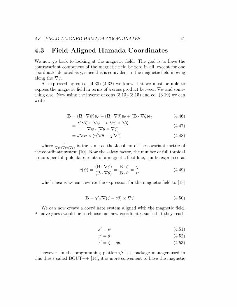
4.3 Field-Aligned Hamada Coordinates
We now go back to looking at the magnetic field. The goal is to have thecontravariant component of the magnetic field be zero in all, except for onecoordinate, denoted as y, since this is equivalent to the magnetic field movingalong the ∇y.
As expressed by eqns. (4.30)-(4.32) we know that we must be able toexpress the magnetic field in terms of a cross product between ∇ψ and some-thing else. Now using the inverse of eqns (3.13)-(3.15) and eq. (3.19) we canwrite
B = (B · ∇ψ)eψ + (B · ∇θ)eθ + (B · ∇ζ)eζ (4.46)
=χ′∇ζ ×∇ψ + υ′∇ψ ×∇ζ
∇ψ · (∇θ ×∇ζ)(4.47)
= J∇ψ × (υ′∇θ − χ′∇ζ) (4.48)
where 1∇ψ·(∇θ×∇ζ) is the same as the Jacobian of the covariant metric of
the coordinate system [10]. Now the safety factor, the number of full toroidalcircuits per full poloidal circuits of a magnetic field line, can be expressed as
q(ψ) =〈B · ∇φ〉〈B · ∇θ〉
=B · ζB · θ
=χ′
υ′(4.49)
which means we can rewrite the expression for the magnetic field to [13]
B = χ′J∇(ζ − qθ)×∇ψ (4.50)
We can now create a coordinate system aligned with the magnetic field.A naive guess would be to choose our new coordinates such that they read
x′ = ψ (4.51)
y′ = θ (4.52)
z′ = ζ − qθ, (4.53)
however, in the programming platform/C++ package manager used inthis thesis called BOUT++ [14], it is more convenient to have the magnetic

42 CHAPTER 4. FIELD ALIGNED COORDINATES
field written in what is called normalized Clebsch form [10]. NormalizedClebsch form means that the magnetic field is represented as [10]
B = e3 × e1 (4.54)
We know that χ′ is a flux function and the Jacobian is also a flux function[13]. This can be shown by requiring that the magnetic field be divergencefree (which it must be according to Maxwells equations), and by taking thedivergence of eq. (4.48), and using several vector rules5 and the fact that χ′
and υ′ are flux functions we have [13]
∇ ·B = ∇J · ∇ψ × (υ′∇θ − χ′∇ζ) = 0 (4.55)
which means that J ‖ ψ, and thus that J is a flux function. This allowsus to define a coordinate that is a flux function, and write the magnetic fieldon normalized Clebsch form. The coordinates are
x =
∫(Jχ′)dψ (4.56)
y = θ (4.57)
z = ζ − qθ (4.58)
and the magnetic field is
B = ∇z ×∇x (4.59)
Note that the shift in z makes y aligned with the magnetic field. Thiscan be explained by holding z constant and moving along y, if you do soyou must move along both θ and ζ. Where the Hamada coordinates wereperiodic, this is no longer the case for the y-coordinate. However we do havewhat is called pseudoperiodicity, which means that
f(x, y + 2π, z) = f(x, y, z − 2πq) (4.60)
We now have a set of field-aligned coordinates true for any solution tothe Grad-Shafranov equation (eq. (4.29)).
5See Appendix B for useful vector identities
4.4. THE CIRCLE EQUILIBRIUM MODEL 43
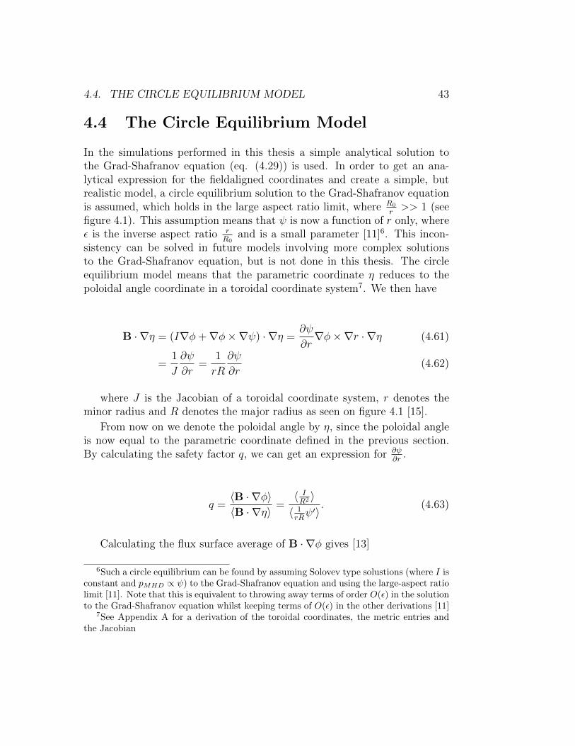
4.4 The Circle Equilibrium Model
In the simulations performed in this thesis a simple analytical solution tothe Grad-Shafranov equation (eq. (4.29)) is used. In order to get an ana-lytical expression for the fieldaligned coordinates and create a simple, butrealistic model, a circle equilibrium solution to the Grad-Shafranov equationis assumed, which holds in the large aspect ratio limit, where R0
r>> 1 (see
figure 4.1). This assumption means that ψ is now a function of r only, whereε is the inverse aspect ratio r
R0and is a small parameter [11]6. This incon-
sistency can be solved in future models involving more complex solutionsto the Grad-Shafranov equation, but is not done in this thesis. The circleequilibrium model means that the parametric coordinate η reduces to thepoloidal angle coordinate in a toroidal coordinate system7. We then have
B · ∇η = (I∇φ+∇φ×∇ψ) · ∇η =∂ψ
∂r∇φ×∇r · ∇η (4.61)
=1
J
∂ψ
∂r=
1
rR
∂ψ
∂r(4.62)
where J is the Jacobian of a toroidal coordinate system, r denotes theminor radius and R denotes the major radius as seen on figure 4.1 [15].
From now on we denote the poloidal angle by η, since the poloidal angleis now equal to the parametric coordinate defined in the previous section.By calculating the safety factor q, we can get an expression for ∂ψ
∂r.
q =〈B · ∇φ〉〈B · ∇η〉
=〈 IR2 〉〈 1rRψ′〉
. (4.63)
Calculating the flux surface average of B · ∇φ gives [13]
6Such a circle equilibrium can be found by assuming Solovev type solustions (where I isconstant and pMHD ∝ ψ) to the Grad-Shafranov equation and using the large-aspect ratiolimit [11]. Note that this is equivalent to throwing away terms of order O(ε) in the solutionto the Grad-Shafranov equation whilst keeping terms of O(ε) in the other derivations [11]
7See Appendix A for a derivation of the toroidal coordinates, the metric entries andthe Jacobian

44 CHAPTER 4. FIELD ALIGNED COORDINATES
Figure 4.1: Toroidal coordinates (note that θ is different from the Hamadaθ)
〈B · ∇φ〉 =χ′
2π
∫ 2π
0
I
R2
dη
B · ∇η=
rχ′I
R0ψ′2π
∫ 2π
0
1
1 + ε cos(η)(4.64)
=rχ′I
R0ψ′2π
2π√1− ε2
. (4.65)
The flux surface average of B · ∇η is
〈B · ∇η〉 =χ′
2π
∫ 2π
0
dη = χ′ (4.66)
We now have an expression for q in terms of flux functions only,
q =rI
R0ψ′√
1− ε2, (4.67)
which gives us an expression for ψ′
ψ′ =rI
R0q√
1− ε2(4.68)

4.4. THE CIRCLE EQUILIBRIUM MODEL 45
We now calculate the angle-like Hamada coordinates for the circle equi-librium model. Recalling eq. (4.36) all we have to calculate is the integral.We have
∫ η
η0
dη
B · ∇η=
r
ψ′
∫ η
η0
R0(1 + ε cos(η))dη =rR0
ψ′[η + ε sin(η)]ηη0 (4.69)
From eq. (4.37) we have the definition of χ′, which in our case leads to
χ′ =ψ′
rR0
(4.70)
so our theta coordinate (eq. (4.36)) becomes
θ = [η + ε sin(η)]ηη0 (4.71)
From eq. (4.45) we have an expression for the ζ-coordinate, which involvestwo integrals. We start by calculating the flux-surface averaged part.
⟨1
R2
⟩=
rχ′
2πψ′
∫ 2π
0
dη
R0(1 + ε cos(η))=
rχ′
2πR0ψ′2π√
1− ε2=
1
R20
√1− ε2
(4.72)
The first integral can then be found by multiplying the flux average of 1R2
by eq. (4.69). The second integral gives us
∫ η
η0
1
R2
dη
B · ∇η=
r
R0ψ′
∫ η
η0
dη
1 + cos(η)(4.73)
Here one has to be careful when solving the definite integral, since itis not possible to solve the indefinite integral and put in the limits, dueto discontinuities in the solution to the indefinite integral. However in thesimulations we only look at the limit between −π + δ and π − δ where thediscontinuities are not present, in which case the solution to the integralabove becomes

46 CHAPTER 4. FIELD ALIGNED COORDINATES
∫ η
η0
1
R2
dη
B · ∇η=
r
R0ψ′
2arctan
(√1−ε1+ε
tan(η2))
√1− ε2
ηη0
(4.74)
which leads to a new expression for ζ,
ζ = φ+Ir
ψ′R0
√1− ε2
([η + ε sin(η)]ηη0 − [2 arctan(
√1− ε1 + ε
tan(η
2))]ηη0)
(4.75)
= φ+ q
[η + ε sin(η)]ηη0 −
[2 arctan
(√1− ε1 + ε
tan(η
2)
)]ηη0
(4.76)
Note that this does not look periodic in 2π in η. That is, however, becausethe definite integral from 0 to 2π is not found by evaluating the indefiniteintegral in the limits, and when evaluating the definite integral from 0 to 2πone finds, that it is in fact periodic.
4.4.1 The Contravariant Hamada Metric
We now move on to calculating the Hamada metric before calculating thefield aligned metric.
In order to calculate the contravariant metric elements of the Hamadacoordinates we must first calculate the gradients of the respective coordinates.Since we work in a circle equilibrium we have, by using the chain rule,
∇x = Jχ′∇ψ = Jχ′ψ′∇r (4.77)
In this section we will be calculating the metric where we use r as the firstcoordinate instead of ψ, since later inclusion of the Jχ′ψ′ prefactors whencalculating the field aligned metric is trivial.
For the first angle-like coordinate we get
∇θ = ∇η + ε cos(η)∇η +1
R0
sin(η)∇r (4.78)

4.4. THE CIRCLE EQUILIBRIUM MODEL 47
For the second angle-like coordinate we define a function
f = 2 arctan
(√1− ε1 + ε
tan(η
2
))
for simplicity. This gives
∇ζ = ∇φ−(q∂
∂rf + f
∂
∂rq − η ∂
∂rq − ∂
∂r(qε) sin(η)
)∇r (4.79)
−(q∂
∂ηf − (1 + ε cos(η))
)∇η
It can be shown that the contravariant metric coefficients for a torus are(see Appendix A for derivation)
grr = 1 (4.80)
gηη =1
r2(4.81)
gφφ =1
R2(4.82)
where R = R0 + r cos(η), and all the off-diagonal metric components arezero. We now derive the contravariant Hamada metric coefficients:

48 CHAPTER 4. FIELD ALIGNED COORDINATES
grr = ∇r · ∇r = 1 (4.83)
gθθ = ∇θ · ∇θ = (1 + ε cos(η))2 · 1
r2+
(cos(η)
R0
)2
(4.84)
gζζ = ∇ζ · ∇· = 1
R2−(q∂
∂rf + f
∂
∂rq − η ∂
∂rq − sin(η)
∂
∂r(qε)
)2
(4.85)
−(q∂
∂ηf − (1 + ε cos(η))
)2
· 1
r2
grθ = ∇r · ∇θ =cos(η)
R0
(4.86)
grζ = ∇r · ∇ζ = η∂
∂rq + sin(η)
∂
∂r(qε)− q ∂
∂rf − f ∂
∂rq (4.87)
gθζ = ∇θ · ∇ζ = − 1
R0
cos(η) · (q ∂∂rf + f
∂
∂rq − η ∂
∂rq − ∂
∂r(qε) sin(η))
(4.88)
− 1
r2(1 + ε cos(η))(q
∂
∂ηf − (1 + ε cos(η)))
Note that gζζ ,grζ and gθζ are not periodic with respect to the poloidalangle, however this is again because the calculated metric elements only holdin the range ]− π, π[. We now have the contravariant Hamada metric whichwill be a help when deriving the field-aligned contravariant Hamada metric.
4.4.2 The Contravariant Field-Aligned Hamada Met-ric
In the same way as we calculated the contravariant Hamada metric coeffi-cients we now calculate the conravariant metric for the field aligned coordi-nates.
The gradients of eqns. (4.56)-(4.58) are:

4.4. THE CIRCLE EQUILIBRIUM MODEL 49
∇x = J∂χ
∂ψ
∂ψ
∂r∇r (4.89)
∇y = ∇θ (4.90)
∇z = ∇ζ − θ ∂∂rq∇r − q∇θ (4.91)
where J denotes the Jacobian of the covariant Hamada metric (the realHamada metric with the first coordinate being ψ). The Jacobian can befound by taking the square root of the inverse of the determinant of thecontravariant Hamada metric and gives
J =rR0
ψ′(4.92)
which means that
∇x = ψ′∇r (4.93)
From this we can calculate the contravariant metric for the field alignedHamada coordinates.
gxx =
(∂
∂rΨ
)2
(4.94)
gyy = gθθ (4.95)
gzz =
(θ∂
∂rq
)2
+ q2gθθ + gζζ + 2qθ∂
∂rqgrθ − 2θ
∂
∂rqgrζ − 2qgθζ (4.96)
gxy =
(∂
∂rΨ
)grθ (4.97)
gxz =
(∂
∂rΨ
)(grζ − θ ∂
∂rqgrr − qgrθ
)(4.98)
gyz = gθζ − θ(∂
∂rq
)grθ − qgθθ (4.99)
The Jacobian for the field aligned metric is the same as for the modifiedHamada metric.

50 CHAPTER 4. FIELD ALIGNED COORDINATES
We now have the metric needed for simulations in field-aligned coor-dinates, which allows us to move on to deriving the modified Hasegawa-Wakatani equations in field aligned geometry.

Chapter 5
The Hasegawa-WakataniEquations
We start this chapter by stating a number of assumptions used on the two-fluid equations in order to derive a simple set of equations for describingthe evolution of a fusion plasma in three dimensions called the Hasegawa-Wakatani equations. Part of the solution to the Hasegawa-Wakatani equa-tions gives rise to drift waves in the direction perpendicular to the magneticfield [16].
5.1 Assumptions
The assumptions are as follows [16,17]:
Assumption 1 TiTe� 1
The ion temperature is much smaller than the electron temperature andcan hence be neglected.
Assumption 2 β = neTeB2
2µ0
� 1
We assume that the magnetic field pressure is much larger than the par-ticle pressure. The plasma is then said to be a low β-plasma.
Assumption 3 E = −∇φ
51
52 CHAPTER 5. THE HASEGAWA-WAKATANI EQUATIONS
Pertubations in the density and potential of the plasma lead to pertu-bations in the magnetic field, however these pertubations are small, so weassume that we have a static magnetic field, and hence that the electric fieldis curl-free.
Assumption 4 k2 � 1λ2D
where λD is the debye length1. We assume that the wave number for thedrift waves is much larger than the inverse Debye length.
Assumption 5 ne = ni = n
Assumption 4 allows us to assume quasi-neutrality which means that thedensity of the electrons and ions is the same.
Assumption 6 n = n0 + n1
The density can be written in terms of a background density and a den-sity pertubation, where n0 is the background density and n1 is the densitypertubation.
Assumption 7 n0 = N0e− xLn
We assume that the background density is of the form n0 = N0e− xLn in the
edge regions of the plasma, where N0 is a constant and Ln is a characteristiclength scale for the density gradient.
Assumption 8 n1
n0∼ eφ
Te∼ ω
ωci� 1
The relative pertubations in the density, the potential and the ion vortic-ity are assumed to be small, where ωci = eB
miis the ion cyclotron frequency.
This assumption means that
ln(n) ≈ ln(n0) +n1
n0
Assumption 9 ωt � ωci
1The Debye length is the average length at which a particle in a plasma is ”shielded”,such that it’s charge approximately cancels with the charges sorrounding it
5.1. ASSUMPTIONS 53
Furthermore we assume that the drift wave frequency, ωt, is much smallerthan the gyrofrequency2 and that the dominant drift perpendicular to themagnetic field is the E ×B-drift and the diamagnetic drift, where the driftwave frequency is a typical timescale of turbulence.
Assumption 10 k‖ � kx ∼ kz
We assume that the variation of the drift waves is mainly in the perpen-dicular direction.
Assumption 11 Pσ = nσTσ,
where κ has been included in Tσ. The electrons and ions are assumed tobe an isothermal fluid.
Assumption 12 ui‖ = 0
The fact that the ion mass is much larger than the electron mass allows usto assume that the ion inertia fixes the ions in the parallel direction, togetherwith assumption 1 this leads to zero velocity for the ions in the direction ofthe magnetic field.
Assumption 13 ∇Tσ∇n0� 1
Temperature gradient effects can be neglected.
Assumption 14 The dominant drift is the 0th order drift
We assume that the dominant drift in the perpendicular direction is the0th order drift i.e. eq. (2.47).
Since we are working in field-aligned coordinates the magnetic field fol-lows straight lines in the y-direction defined earlier. All differential vectoroperators in the following sections denote the operators in curvilinear geom-etry as defined in the last section of chapter 3.
2For a detailed description of typical plasma frequencies see books such as [9], [6]and [18]
54 CHAPTER 5. THE HASEGAWA-WAKATANI EQUATIONS
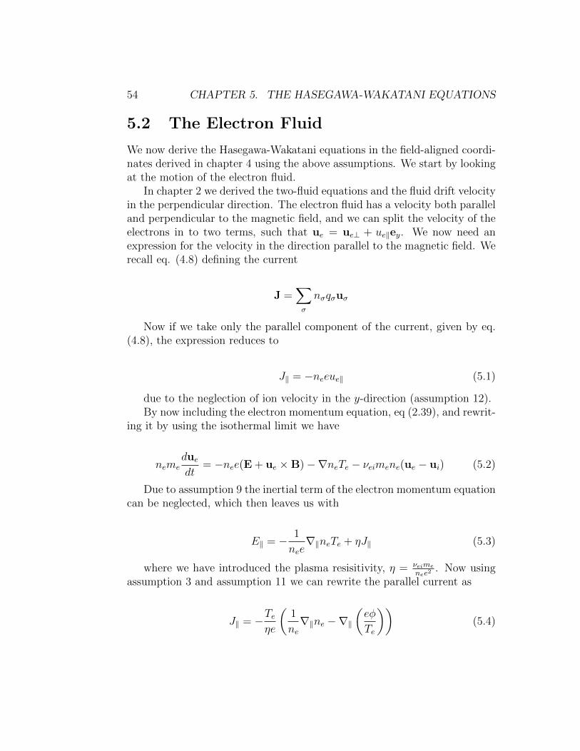
5.2 The Electron Fluid
We now derive the Hasegawa-Wakatani equations in the field-aligned coordi-nates derived in chapter 4 using the above assumptions. We start by lookingat the motion of the electron fluid.
In chapter 2 we derived the two-fluid equations and the fluid drift velocityin the perpendicular direction. The electron fluid has a velocity both paralleland perpendicular to the magnetic field, and we can split the velocity of theelectrons in to two terms, such that ue = ue⊥ + ue‖ey. We now need anexpression for the velocity in the direction parallel to the magnetic field. Werecall eq. (4.8) defining the current
J =∑σ
nσqσuσ
Now if we take only the parallel component of the current, given by eq.(4.8), the expression reduces to
J‖ = −neeue‖ (5.1)
due to the neglection of ion velocity in the y-direction (assumption 12).By now including the electron momentum equation, eq (2.39), and rewrit-
ing it by using the isothermal limit we have
nemeduedt
= −nee(E + ue ×B)−∇neTe − νeimene(ue − ui) (5.2)
Due to assumption 9 the inertial term of the electron momentum equationcan be neglected, which then leaves us with
E‖ = − 1
nee∇‖neTe + ηJ‖ (5.3)
where we have introduced the plasma resisitivity, η = νeimenee2
. Now usingassumption 3 and assumption 11 we can rewrite the parallel current as
J‖ = −Teηe
(1
ne∇‖ne −∇‖
(eφ
Te
))(5.4)
5.2. THE ELECTRON FLUID 55
Recalling eq. (2.47) we can now write the total flow velocity of the elec-tron fluid3
ue =E×B
B2+∇Pσ ×B
neeB2− 1
neeJ‖ (5.5)
Taking a look at the electron continuity equation we have, from eq. (2.38),
∂ne∂t
+∇ · (neue) = 0 (5.6)
The dot product between the diamagnetic drift and the gradient of thedensity is zero due to assumption 13, and the divergence of the perpendiculardrifts is zero, so the perpendicular part of the second term on the left handside reads
∇ · (neue)⊥ =E×B
B2· ∇ne (5.7)
The divergence of the parallel part is given by
∇‖ · (neu‖) = −1
e∇‖ · J‖ (5.8)
Rewriting the electron continuity equation and using quasi-neutrality wethen have
∂n
∂t− ∇φ×B
B2· ∇n =
1
e∇‖ · J‖ (5.9)
defining the convective derivative in terms of the E × B-drift as DDt
=∂∂t
+ uE · ∇, the expression is simplified to
D
Dtn =
1
e∇‖ · J‖ (5.10)
This equation in combination with the expression for the parallel currentis the first modified Hasegawa-Wakatani equation4.
3The first order drift can be neglected for electrons due to ωce � ωci, however the ionshave a larger mass than electrons
4Modified due to the fact that the original set of equations assume a slab coordinatesystem

56 CHAPTER 5. THE HASEGAWA-WAKATANI EQUATIONS
5.3 The Ion Fluid
When finding the second equation of the Hasegawa-Wakatani model we uti-lize the assumption that the ions are cold, thus enabling us to neglect thediamagnetic drift and the drift parallel to the magnetic field. The only re-maining 0th order drift is then the E×B-drift. The first order drift for theions is given by eq. (2.48) as
ui = − mi
eB2
(∂t −
(∇φ×B
B2· ∇))∇φ− ∇φ×B
B2(5.11)
Taking a look at the ion continuity equation, eq. (2.38), and plugging inthe ion velocity we get
− 1
Bωci
(∂t −
∇φ×B
B2· ∇)∇2φ =
−∂tn+
(∇φ×B
B2+
1
Bωci
(∂t −
∇φ×B
B2· ∇)∇φ)· ∇n (5.12)
the 1Bωci
(∂t − ∇φ×BB2 · ∇
)∇φ term on the right hand side, also called the
polariazation drift, is much smaller than the E×B-drift due to assumption14 and can be neglected. Introducing the convective derivative on both sides,and substituting eq. (5.10) in to the right hand side we get
D
Dt
∇2φ
Bωci=
1
en∇‖ · J‖ (5.13)
This is the second Hasegawa-Wakatani equation. We now have a set ofclosed partial differential equations.
5.4 Normalizing the Hasegawa-Wakatani equa-
tions
When running simulations it is often convenient to normalize the equations.In order to normalize the Hasegawa-Wakatani equations, eq. (5.10) and eq.

5.4. NORMALIZING THE HASEGAWA-WAKATANI EQUATIONS 57
(5.13), it is convenient to rewrite them. We start by using assumption 6 andusing assumption 7 to rewrite the parallel current, eq. (5.4), to
J‖ = −Teηe
(∇‖(
ln(n0) +n1
n0
)−∇‖(eφ
Te
))(5.14)
where we have used ∇ ln(n) = 1n∇n. Using assumption 8, the expression
for the current simplifies to
J‖ = −Teηe
(∇‖(n1
n0
)−∇‖
(eφ
Te
))(5.15)
We now move on to rewriting the electron fluid eqaution (eq. (5.10)).Dividing eq. (5.10) by n on both sides gives
1
n
D
Dtn =
1
ne∇‖J‖ (5.16)
writing n = n0 + n1 and using once again that ∇ ln(n) = 1n∇n we have
D
Dtln(n0 + n1) =
1
e(n0 + n1)∇‖J‖ (5.17)
using assumption 8 we can write
1
en0(1 + n1
n0)≈ 1
en0
(5.18)
and
D
Dt
(ln(n0) +
n1
n0
)=
1
en0
∇‖ · J‖ (5.19)
Eq. (5.13) can in the same way be rewritten to
D
Dt
∇2φ
Bωci=
1
en0
∇‖ · J‖ (5.20)

58 CHAPTER 5. THE HASEGAWA-WAKATANI EQUATIONS
Using the rewritten equations we now start the normalization. We intro-duce the normalized quantities
l =l
ρs, t = ωcit, φ =
eφ
Te, n =
n1
n0
, ∇ = ρs∇
where l denotes any length parameter and ρs =√TemieB
is the ion gyroradiusat the electron temperature Te. Plugging this in to the Hasegawa-Wakataniequations (eqns. (5.19) and (5.20)) and utilizing that ∂tn0 = 0 and addinga diffusion and viscosity term [17] to them, we end up with the normalizedHasegawa-Wakatani equations
(∂t + uE · ∇)n+ uE · ∇(ln(n0)) = C∇‖ · ∇‖(n− φ) + µ∇2n (5.21)
(∂t + uE · ∇)∇2φ = C∇‖ · ∇‖(n− φ) + µ∇4φ (5.22)
where
C =Te
ηe2n0ωciρ2s(5.23)
This normalization, however, also means that we must normalize themetric elements used in the differential operators. Utilizing that in the largeaspect ratio limit we have I ≈ R0B0 [11,13], we have as an expression for ψ′:
ψ′ =rB0
q√
1− ε2. (5.24)
The safety factor is unitless, and the SI units of ψ′ is then tesla timesmetres. This leads to the normalization
gxx = ∇x · ∇x = ρ2sB20 g
xx (5.25)
gyy = ∇y · ∇y =1
ρ2sgyy (5.26)
gzz =1
ρ2sgzz (5.27)
gxy = B0gxy (5.28)
gxz = B0gxz (5.29)
gyz =1
ρ2sgyz (5.30)

5.4. NORMALIZING THE HASEGAWA-WAKATANI EQUATIONS 59
We now have a set of normalized, closed partial differential equations.The next step is to analyze the dynamics of the system described by theequations, and this is done by simulations using the BOUT++ platform.

60 CHAPTER 5. THE HASEGAWA-WAKATANI EQUATIONS
Chapter 6
Simulations of theHasegawa-Wakatani System
In this chapter we carry out simulations of the Hasegawa-Wakatani equationsin our field-aligned system and define the numerical values for the field-aligned metric.
6.1 The Metric
The metric used in the simulations is the same as the circle equilibrium metricderived in chapter 4. We use the local approximation, which means that allr-dependencies are held constant while still including derivatives with respectto r, such that for instance q(r) = Const and ∂q
∂r= Const 6= 0. This leaves
us with metric components that are only functions of the y-parameter.In order to carry out the simulations we create a so-called grid file, which is
a file including all necessary information about the coordinates. The spacingbetween each field-aligned coordinate and its neighbour is the same every-where, which means the spacing is equidistant.1
In the metric there are several η-dependencies which we want expressedas funtions of y. However y = θ = η + ε sin(η), so finding an analyticalexpression for η in terms of y is not straightforward. This is solved by addingan iterative newton solver [19] in the grid file created. The solver finds thevalues of η for which y − η − ε sin(η) = 0 with equidistant gridspacing in y.In figure 6.1 we see how η is shifted with respect to θ when ε = 0.125.
1For a detailed description of the finite difference methods used in BOUT++ see [12]
61

62CHAPTER 6. SIMULATIONS OF THE HASEGAWA-WAKATANI SYSTEM
Figure 6.1: η plotted against θ
In our metric we assume q(r) to be proportional to r2, while requiringthat q is still unitless.
For the simulations carried out in this chapter we have looked at a smallTokamak with a major radius of R0 = 1 m and a minor radius of r ≈ 0.125m.
Table 6.1: Values for the metric
symbol valueLowest value for the minor radius rmin 0.1 mHighest value for the minor radius rmax 0.15 mAverage and assumed value for the minor radius r0 0.125 mMajor radius R0 1 m
The safety factor as a function of r q 2 + 7 rR0
+ r2
R20
The derivative of the safety factor with respect to r q′ 7R0
+ 2 rR2
0
In table 6.1 all values used to derive the field-aligned metric used in thesimulations performed in this chapter can be seen.
Plugging the values from table 6.1 into the metric elements of eqns.

6.1. THE METRIC 63
Figure 6.2: The metric coefficients of the field-aligned coordinates as func-tions of y

64CHAPTER 6. SIMULATIONS OF THE HASEGAWA-WAKATANI SYSTEM
Figure 6.3: The metric coefficients depending on q′ as functions of y
(4.94)-(4.99) gives figure 6.2. All the metric coefficients are shown as func-tions of y in the range y =]−π, π[. As seen, the metric elements containing zderivatives are not necessarily periodic nor continuous. The non-periodicityis due to the shift by qθ in the z-direction (eq. (4.58)) and the discontinuityis due to the discontinuous nature of the integral calculated for the ζ Hamadacoordinate (eq. (4.74)). Furthermore note that the three z-dependent met-ric elements are highly dependent on the derivative of the safety factor withrespect to r, in fact if we have q′ = 0 all the metric elements end up periodicas seen in figure 6.3.
With our evaluation of the field-aligned metric complete we are now ableto move on to a simple test simulation of the metric involving diffusion inthe ∇y-direction.
6.2. SIMPLE DIFFUSION 65
6.2 Simple Diffusion
In this short section we simulate the behaviour of simple diffusion parrallel tothe magnetic field in the case of a rational q, and in the case of an irrationalq.
The diffusion equation evaluated is simply
∂tN = D‖∇2‖N (6.1)
where N is a particle density, and D‖ is a constant.Due to the shift in the z-coordinate being by 2πqθ as seen in eq. (4.58)
and the pseudo-periodicity expressed by eq. (4.60) we should see that for arational q a magnetic field line will eventually close in on itself, where for anirrational q, the magnetic field line will never close in on itself, resulting in amagnetic field line covering a whole surface. This means that looking at twofield lines for a choice of rational q with a different density on each field line,there should be no diffusion between the two field lines, where the oppositeshould be the case for an irrational choice of q.
Figure 6.4 shows diffusion at three different times with a diffusion constantof D‖ = 1000 and with a rational choice of q. The density is distributed, suchthat each field line has a constant density different from the other field line.As seen from the plots there is no diffusion from one field line to the other,just as expected.
Figure 6.5 shows diffusion at three different times with a diffusion constantof D‖ = 1000 and with an irrational choice of q and a distribution of density,such that each field line has a constant density different from the other fieldline. As expected the density evens out among the two field lines.
6.2.1 Cross-section and Interpolation
When investigating data it is often convenient to look at 2-dimensional crosssections with one coordinate held fixed. Imagine we want to look at a crosssection of the data in toroidal coordinates at φ = 0. If the simulation wasdone in a toroidal coordinate system with an equidistant grid, this wouldbe straightforward, however, our simulations were done in a non-toroidalsystem, and the gridpoints are thus not necessarily uniformly distributedalong a constant φ-plane. However there are various ways to interpolate

66CHAPTER 6. SIMULATIONS OF THE HASEGAWA-WAKATANI SYSTEM
data down to the poloidal plane in a toroidal geometry, and we simply usepythons built-in interpolator when processing the data2.
In order to get results in a more visualizable coordinate system we mapthe data back to toroidal coordinates. We have a one-to-one map of the threefield-aligned coordinates to toroidal coordinates, such that (xfa, yfa, zfa) →(r, η, φ), using the values for the toroidal coordinates in terms of the field-aligned coordinates we are able to map back to toroidal coordinates. Thishas been utilised in a simulation run using a 32x64x36 grid, with an initialdistribution in the z-direction given by the function N0 = 1 + sin( z
2) in the
range ] − π, π[ for z, with diffusion in the y-direction, an irrational q andD‖ = 1000. Figure 6.6 shows the simulations for a cross section at φ = 0 andφ = π, where φ is the toroidal angle, at times 10 s, 4000 s and 20000 s. Thefigure shows that with time the density is evenly distributed as expected.
These simple diffusion tests have shown that the metric inputs behave asexpected and that the results given in the field-aligned coordinates can bemapped back to a toroidal system, which validates our metric and numericalimplementation.
2While the simulations where done using C++ and the BOUT++ [14] platform, thepost processing was done in Python
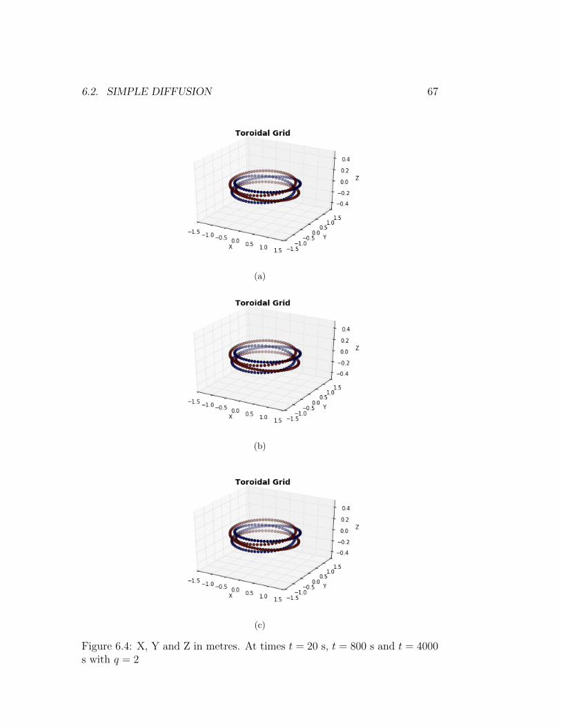
6.2. SIMPLE DIFFUSION 67
(a)
(b)
(c)
Figure 6.4: X, Y and Z in metres. At times t = 20 s, t = 800 s and t = 4000s with q = 2

68CHAPTER 6. SIMULATIONS OF THE HASEGAWA-WAKATANI SYSTEM
(a)
(b)
(c)
Figure 6.5: X, Y and Z in metres. At times t = 20 s, t = 800 s and t = 4000s with q = π
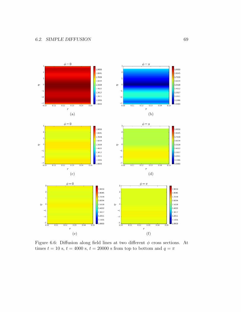
6.2. SIMPLE DIFFUSION 69
(a) (b)
(c) (d)
(e) (f)
Figure 6.6: Diffusion along field lines at two different φ cross sections. Attimes t = 10 s, t = 4000 s, t = 20000 s from top to bottom and q = π
70CHAPTER 6. SIMULATIONS OF THE HASEGAWA-WAKATANI SYSTEM
6.3 The Dispersion Relation and Unstable Modes
In order to investigate the growth rate of unstable modes it is convenientto look at the linearized limit of the Hasegawa-Wakatani equations. Doingthis in a slab geometry is straightforward and gives a dispersion relation,however it is not straightforward in the field-aligned geometry used for thesimulations performed in this chapter. Due to the complexity of the curvi-linear coordinates we restrict our investigation to a slab geometry. This willgive an indication of the growth-rates of the different modes in curvilineargeometry3. Slab geometry is defined as a cartesian coordinate system with yas the magnetic field axis4.
When we assume that the geometry is a slab, the term uE · ∇n0 can berewritten to [16]
uE · ∇n0 =1
LnB0
∂
∂zφ (6.2)
The linearized Hasegawa-Wakatani equations are then [18]
∂tn+ ∂zφ = −C∂2y(φ− n) + µ∇2⊥n (6.3)
∂t∇2⊥φ = −C∂2y(φ− n) + µ∇4
⊥φ (6.4)
where C is given by
C =TeLn
ηe2n0ωciρ3s(6.5)
where the perpendicular length scales are normalized with ρs and the par-allel length scales are normalized with Ln. The reason for this normalizationis the different typical length scales perpendicular to the magnetic field andalong the magnetic field.
Assuming plane wave solutions to eqns (6.3)-(6.4) and ignoring electronviscosity gives the dispersion relation [18]
3Things like magnetic shear, etc. are not included4usually z, but BOUT++ uses y

6.3. THE DISPERSION RELATION AND UNSTABLE MODES 71
ω2 + iω
(Ck2y
(1 +
1
k2⊥
)+ µk2⊥
)− Ck2y
(ikzk2⊥
+ µk2⊥
)= 0 (6.6)
In the limit where C → ∞ we get
ω =kz
1 + k2⊥− i µk4⊥
1 + k2⊥(6.7)
The limit where C → 0 gives
ω = −iµk2⊥, 0 (6.8)
We see that both limits have a net negative of the imaginary parts, whichresults in a damping of the unstable modes [18]. This means that we have astable solution in both limits, and furthermore that the limit where C → ∞simply gives the standard result for drift waves in the z-direction [18].
The solution to the total dispersion relation is found to be
ω =−i(Ck2yk⊥ + µk3⊥ + Ck2y)
2k⊥(6.9)
±√−k4y(k⊥ + 1)2C2 + 2k2yC(k4⊥µ− k3⊥µ)− µ2k6⊥ + 4k2yCiω∗
2k⊥
As seen the solution includes two branches, however the branch with=(ω) < 0 is damped out by the negative imaginary part while the otherbranch is unstable, and drives the instabilities [18]. With C = 1, µ = 0 andkx = 0, we plot the dispersion relation for the unstable branch (=(ω) > 0) ,which is illustrated in figure 6.7.
To better illustrate the growth-rate dependencies on k, we have plottedthe cross sections of the imaginary frequency illustrated in figure 6.7 and infigure 6.8. As seen in the figure, the imaginary part (blue line) has a peak ata lower wave number for higher C, and a faster decay after the peak. Howeverfor low C the peak of the imaginary part is at a lower frequency. This meansthat the peaks of both the real and imaginary parts go to zero for C → 0, and
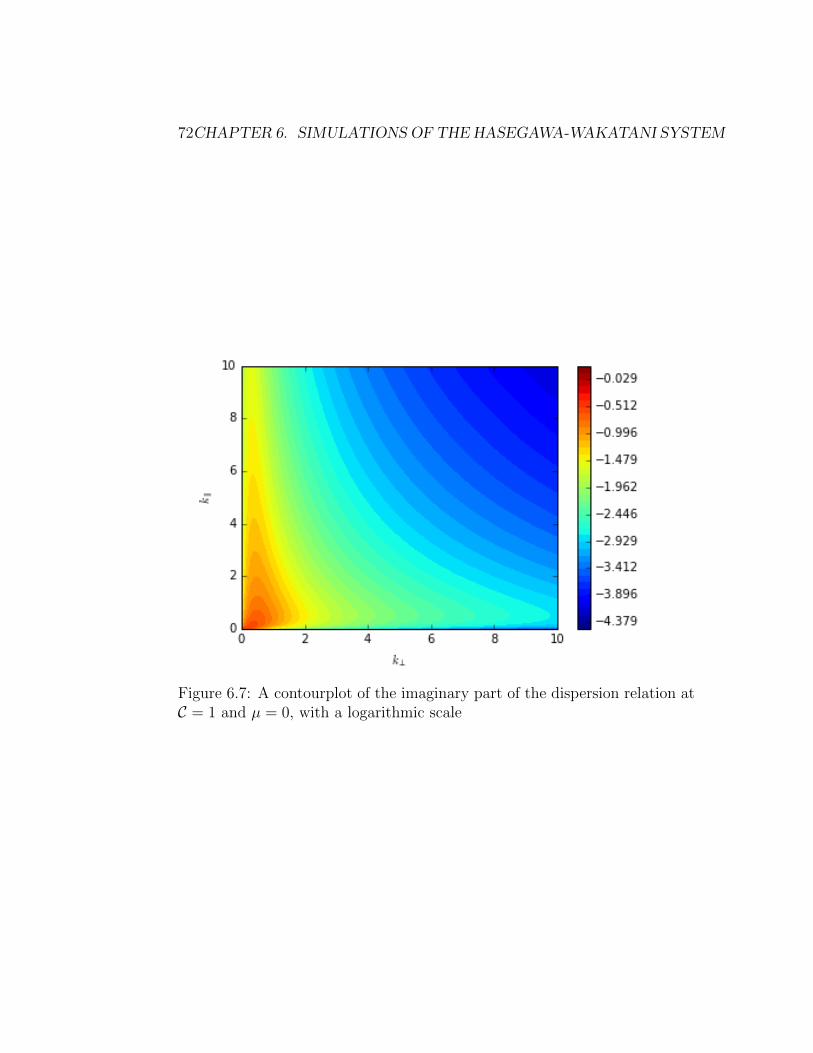
72CHAPTER 6. SIMULATIONS OF THE HASEGAWA-WAKATANI SYSTEM
Figure 6.7: A contourplot of the imaginary part of the dispersion relation atC = 1 and µ = 0, with a logarithmic scale

6.3. THE DISPERSION RELATION AND UNSTABLE MODES 73
the peak of the imaginary part goes to zero as C → ∞. The growth rate forthe unstable modes is seen to have the maximum peak value around C = 1.
Figure 6.9 shows the maximum frequency of the imaginary part of theperpendicular wave number, k⊥, decaying fast for higher values of C. ForC → 0 the peak of both the real and the imaginary part goes to zero resultingin a stable solution.
Whilst this mainly tells us something about the Hasegawa-Wakatani modelin a slab geometry, the results for a curvilinear geometry should be similar,with the drift wave instabilities peaking at a finite C.
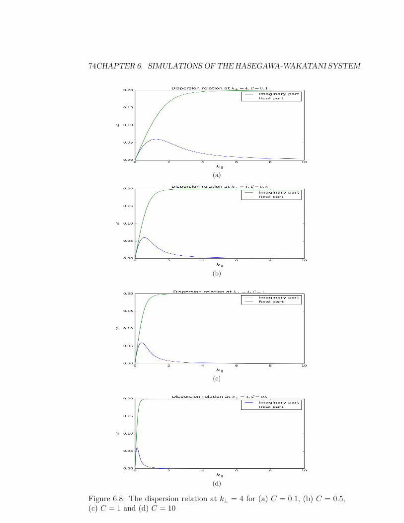
74CHAPTER 6. SIMULATIONS OF THE HASEGAWA-WAKATANI SYSTEM
(a)
(b)
(c)
(d)
Figure 6.8: The dispersion relation at k⊥ = 4 for (a) C = 0.1, (b) C = 0.5,(c) C = 1 and (d) C = 10

6.3. THE DISPERSION RELATION AND UNSTABLE MODES 75
(a)
(b)
(c)
(d)
Figure 6.9: The dispersion relation at k‖ = 4 for (a) C = 0.1, (b) C = 0.5,(c) C = 1 and (d) C = 10
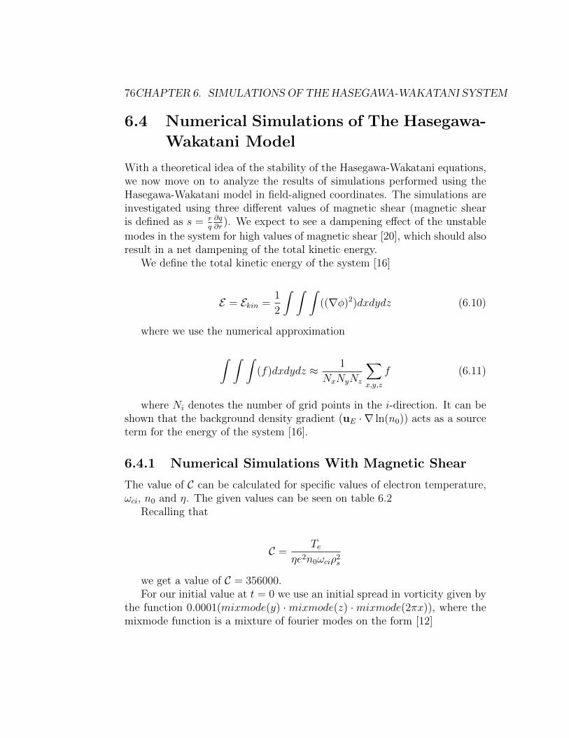
76CHAPTER 6. SIMULATIONS OF THE HASEGAWA-WAKATANI SYSTEM
6.4 Numerical Simulations of The Hasegawa-
Wakatani Model
With a theoretical idea of the stability of the Hasegawa-Wakatani equations,we now move on to analyze the results of simulations performed using theHasegawa-Wakatani model in field-aligned coordinates. The simulations areinvestigated using three different values of magnetic shear (magnetic shearis defined as s = r
q∂q∂r
). We expect to see a dampening effect of the unstable
modes in the system for high values of magnetic shear [20], which should alsoresult in a net dampening of the total kinetic energy.
We define the total kinetic energy of the system [16]
E = Ekin =1
2
∫ ∫ ∫((∇φ)2)dxdydz (6.10)
where we use the numerical approximation
∫ ∫ ∫(f)dxdydz ≈ 1
NxNyNz
∑x,y,z
f (6.11)
where Ni denotes the number of grid points in the i-direction. It can beshown that the background density gradient (uE · ∇ ln(n0)) acts as a sourceterm for the energy of the system [16].
6.4.1 Numerical Simulations With Magnetic Shear
The value of C can be calculated for specific values of electron temperature,ωci, n0 and η. The given values can be seen on table 6.2
Recalling that
C =Te
ηe2n0ωciρ2s
we get a value of C = 356000.For our initial value at t = 0 we use an initial spread in vorticity given by
the function 0.0001(mixmode(y) ·mixmode(z) ·mixmode(2πx)), where themixmode function is a mixture of fourier modes on the form [12]

6.4. NUMERICAL SIMULATIONS OF THE HASEGAWA-WAKATANI MODEL77
Table 6.2: Values used for the simulation
symbol valueParticle background number density n0 1019
Electron temperature Te 100 eVThe ion cyclotron frequency ωci 47904191 s−1
The plasma resisitivity η 1.7 · 10−6
The ion larmor radiues at electron temperature Te ρs 0.0014 mThe electron charge e 1.6 · 10−19 CThe background magnetic field B0 1 T
mixmode(x) =14∑i=1
1
(1 + |i− 4|)2cos[ix+ φ], (6.12)
where φ is a random phase between -π and π. The boundaries in the y-and z-directions are periodic and on the x-coordinates boundaries we imposedirichlet boundaries5 [19] of values 0. The same boundaries are applied to thenormalized density n. The grid used is an equidistant 66×16×512 grid usingthe field-aligned coordinates derived in chapter 4, with input parameters forthe metric and coordinates given in table 6.1. The timestep used was t = 100corresponding to t = 100
ωci. The background density gradient was set to be
∇(log(n0)) = ∇(−1 · x).Figure 6.10 shows the total normalised kinetic energy in the system as
a function of time with and without kinetic energy in the parallel direction.As seen from the plot the kinetic energy in the parallel direction contributeswith almost nothing, which means the drift waves and turbulence mainlyresults in motion perpendicular to the magnetic field.
At approximately t = 800 the kinetic energy of the system starts growingexponentially up untill approximately t = 8700. In this region the kineticenergy is concentrated in the stable wave numbers, with a resulting drift inthe z-direction. A snapshot during this time period at a cross section ofy = 0.25π can be seen in figure 6.11.
5For the finite difference methods used in BOUT++ see [19] and [12]

78CHAPTER 6. SIMULATIONS OF THE HASEGAWA-WAKATANI SYSTEM
Figure 6.10: The kinetic energy as a function of time.

6.4. NUMERICAL SIMULATIONS OF THE HASEGAWA-WAKATANI MODEL79
Figure 6.11: The normalized values for n, φ ,∇2φ and J‖ at time t = 6000
with ∂q∂r
= 7.25

80CHAPTER 6. SIMULATIONS OF THE HASEGAWA-WAKATANI SYSTEM
The period from time t = 8700 and onward denotes the state of thesystem where the total kinetic energy of the system is saturated. In thesaturated state the system becomes turbulent and random oscillations in thetotal kinetic energy are observed. Figure 6.12 shows a snapshot during thestart of the turbulent time period at a cross section of y = 0.25π. Figure6.13 shows a snapshot well into the turbulent time period at a cross sectionof y = 0.25π. As seen in figure 6.13 it seems that φ goes in to a state withelongated modes late in the turbulent time period.
As mentioned earlier the magnetic shear is expected to have a positiveinfluence on the stability of the system. In order to investigate this influence,we compare these results to a system with no magnetic shear and a systemwith stronger magnetic shear.

6.4. NUMERICAL SIMULATIONS OF THE HASEGAWA-WAKATANI MODEL81
Figure 6.12: The normalized values for n, φ ,∇2φ and J‖ at time t = 10600
with ∂q∂r
= 7.25

82CHAPTER 6. SIMULATIONS OF THE HASEGAWA-WAKATANI SYSTEM
Figure 6.13: The normalized values for n, φ ,∇2φ and J‖ at time t = 35000
with ∂q∂r
= 7.25

6.4. NUMERICAL SIMULATIONS OF THE HASEGAWA-WAKATANI MODEL83
Figure 6.14: The kinetic energy as a function of time.
Comparisons with no magnetic shear
In this subsection we investigate the case where no magnetic shear is present,that is we set ∂q
∂r= 0, whilst not changing any other parameters. What we
expect is a less stable Hasegawa-Wakatani system, that reaches a saturatedstate faster than a Hasegawa-Wakatani system with shear. We also expecthigher total kinetic energy in the saturated state due to more unstable mo-tion.
Figure 6.14 shows the total normalized kinetic energy of the system withno shear. At approximately t = 800 the kinetic energy of the system startsgrowing exponentially up untill approximately t = 8000. Compared to theprevious simulation it reaches the saturated state a bit faster. By zoomingin at time t = (30000− 45000) for the total kinetic energy with and withoutmagnetic shear we get figures 6.15 for no magnetic shear, and figure 6.16 forthe case with magnetic shear. It is quite clear that the total kinetic energy

84CHAPTER 6. SIMULATIONS OF THE HASEGAWA-WAKATANI SYSTEM
Figure 6.15: The kinetic energy as a function of time.
in the saturated state in the case with no magnetic shear is larger.Figure 6.17 shows the system with no shear at time t = 6000 and y =
0.25π. Comparing figure 6.17 with figure 6.11 it is seen that the densityprofile, the electric potential and the vorticity is shifted in the z-direction forhigher r when magnetic shear is present, whereas it is not shifted in the casewithout magnetic shear.
Figure 6.18 shows the system with no magnetic shear at the initial stateof the turbulent time period and figure 6.19 shows the same system well intothe turbulent time period, both at y = 0.25π. Compared to the system withshear, φ does not seem to form the same elongated modes.
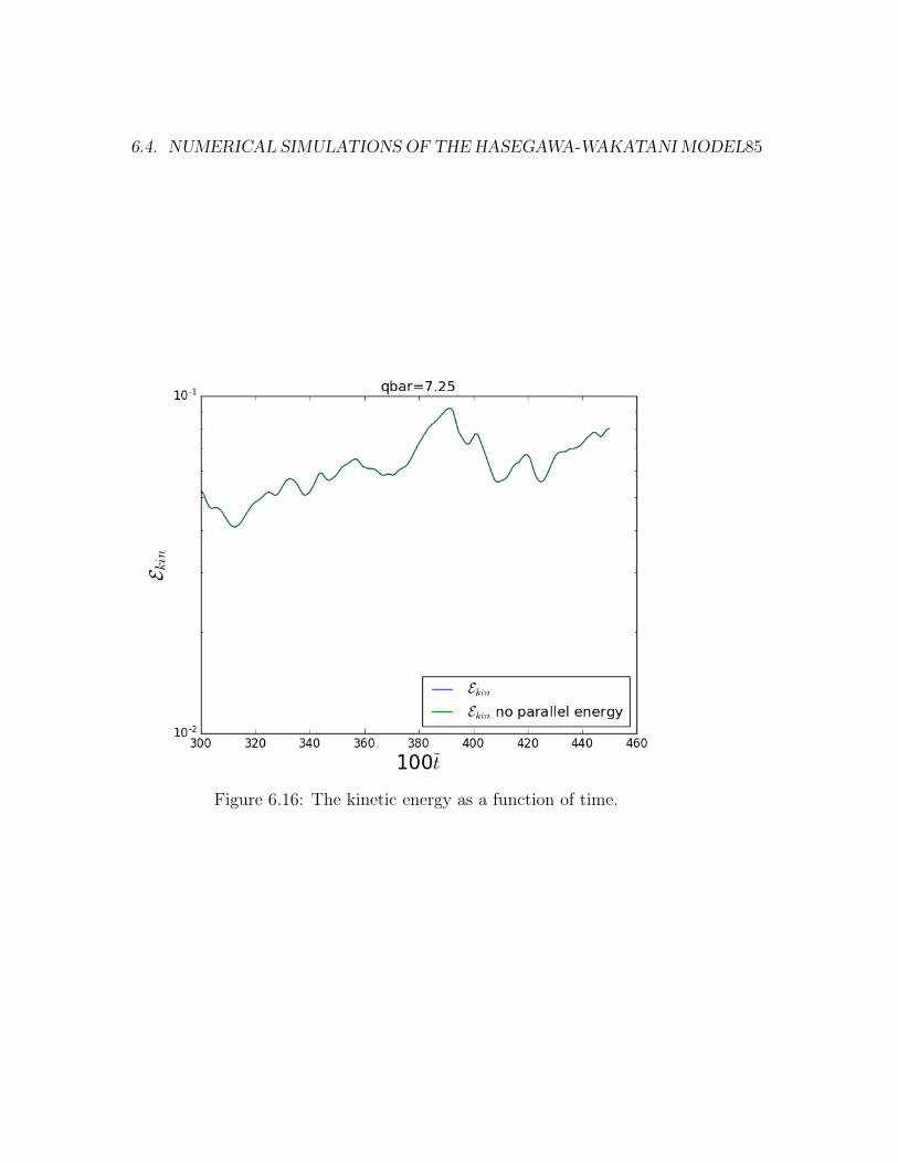
6.4. NUMERICAL SIMULATIONS OF THE HASEGAWA-WAKATANI MODEL85
Figure 6.16: The kinetic energy as a function of time.
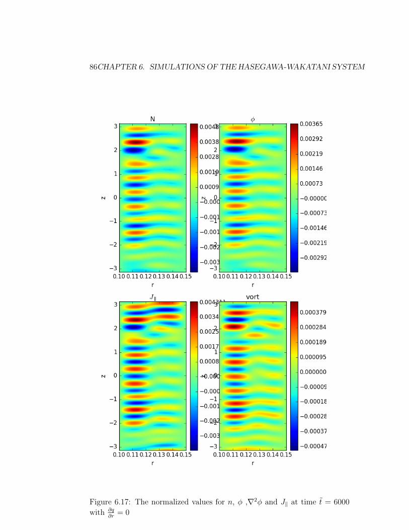
86CHAPTER 6. SIMULATIONS OF THE HASEGAWA-WAKATANI SYSTEM
Figure 6.17: The normalized values for n, φ ,∇2φ and J‖ at time t = 6000
with ∂q∂r
= 0

6.4. NUMERICAL SIMULATIONS OF THE HASEGAWA-WAKATANI MODEL87
Figure 6.18: The normalized values for n, φ ,∇2φ and J‖ at time t = 10600
with ∂q∂r
= 0

88CHAPTER 6. SIMULATIONS OF THE HASEGAWA-WAKATANI SYSTEM
Figure 6.19: The normalized values for n, φ ,∇2φ and J‖ at time t = 35000
with ∂q∂r
= 0
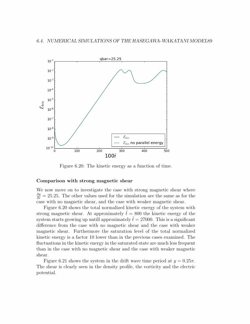
6.4. NUMERICAL SIMULATIONS OF THE HASEGAWA-WAKATANI MODEL89
Figure 6.20: The kinetic energy as a function of time.
Comparison with strong magnetic shear
We now move on to investigate the case with strong magnetic shear where∂q∂r
= 25.25. The other values used for the simulation are the same as for thecase with no magnetic shear, and the case with weaker magnetic shear.
Figure 6.20 shows the total normalized kinetic energy of the system withstrong magnetic shear. At approximately t = 800 the kinetic energy of thesystem starts growing up untill approximately t = 27000. This is a significantdifference from the case with no magnetic shear and the case with weakermagnetic shear. Furthermore the saturation level of the total normalizedkinetic energy is a factor 10 lower than in the previous cases examined. Thefluctuations in the kinetic energy in the saturated state are much less frequentthan in the case with no magnetic shear and the case with weaker magneticshear.
Figure 6.21 shows the system in the drift wave time period at y = 0.25π.The shear is clearly seen in the density profile, the vorticity and the electricpotential.

90CHAPTER 6. SIMULATIONS OF THE HASEGAWA-WAKATANI SYSTEM
Figure 6.21: The normalized values for n, φ ,∇2φ and J‖ at time t = 10600
with ∂q∂r
= 25.25

6.4. NUMERICAL SIMULATIONS OF THE HASEGAWA-WAKATANI MODEL91
Figure 6.22: The normalized values for n, φ ,∇2φ and J‖ at time t = 35000
with ∂q∂r
= 25.25

92CHAPTER 6. SIMULATIONS OF THE HASEGAWA-WAKATANI SYSTEM
Figure 6.22 shows the system in the turbulent time period at y = 0.25πthe elongated modes in the electric potential are even more visible now.
It is clear that the magnetic shear has a stabilizing effect on the systemand this can be utilized when building a fusion plasma device.

Chapter 7
Conclusion
In order to accurately describe a fusion plasma 3D effects of the magneticfield must be taken in to account. A 3D model using a coordinate systemaligned with the magnetic field takes these effects in to account and leadsto high resolution of the effects with a coarse grid in the magnetic field linedirection.
To create a 3D model of a fusion plasma the shape of the magnetic fieldwas described in detail, from which a coordinate system aligned with themagnetic field was derived. A metric, involving all necesarry informationabout the magnetic field structure, was created from the field-aligned co-ordinates. The Hasegawa-Wakatani model was then investigated using thefield-aligned coordinate system.
A simple diffusion test was carried out in order to validate the model andprove the ability of mapping the results in field-aligned coordinates back toa toroidal coordinate system.
Simulations involving three different cases of the derived equations wereinvestigated using the BOUT++ [14] platform for writing the code, one witha magnetic shear of ∂q
∂r= 7.25, one with no shear and one with a shear of
∂q∂r
= 25.25. Significant differences were seen, where the magnetic shear wasshown to have a stabilizing effect on the system.
The 3D model showed promising results as a basis for future simulationsin three dimensions.
93

94 CHAPTER 7. CONCLUSION
7.1 Future Prospects
Creating a coordinate system aligned with the magnetic field is a complicatedand tedious affair, however with this succesfully done, and immediate effectsresulting from the properties of the magnetic field seen, the 3D model createdin this thesis seems to be a great basis for future work using a field alignedsystem.
The model investigated in this thesis was the simplified Hasegawa-Wakatanimodel which includes assumptions such as zero ion temperature, which doesnot necesarrily hold in real fusion devices. Future works may be done usingmore complex systems involving finite ion temperature and other neglectedeffects, such as temperature gradients and parallel ion velocity.
During the simulations, the local approximation was used, which onlyholds for flat gradients or a very thin slab in the r-direction. Future worksmay want to include global effects of r and a first step could be to investigatethe differences between a model using the local approximation and a globalmodel.
The 3D model used for the simulations assumed a circle equilibrium solu-tion to the Grad-Shafranov equation in order to have an analytical expressionfor the field-aligned metric. However this holds an inconsistency of O(ε) withε = r
R0and future works may set out to investigate more complex models
with more realistic solutions to the Grad-Shafranov equation.

Appendix A
Toroidal Metric Coefficients
Using the Cartesian metric where
gxx = 1 (A.1)
gyy = 1 (A.2)
gzz = 1 (A.3)
and the off-diagonal terms are 0 it is pretty straightforward to determinethe metric for a toroidal coordinate system. Defining the coordinates wehave:
x = (R0 + r cos(η)) sin(φ) (A.4)
y = (R0 + r cos(η)) cos(φ) (A.5)
z = r sin(η), (A.6)
where x, y and z are the usual Cartesian coordinates, R0 is the majorradius, r is the minor radius, η is the poloidal angle and φ is the toroidalangle.
Writing the set of toroidal coordinates in terms of cartesian coordinateswe solve the three equations with three unknowns.
φ = arcsin(x
R0 + r cos(η)) (A.7)
so
95
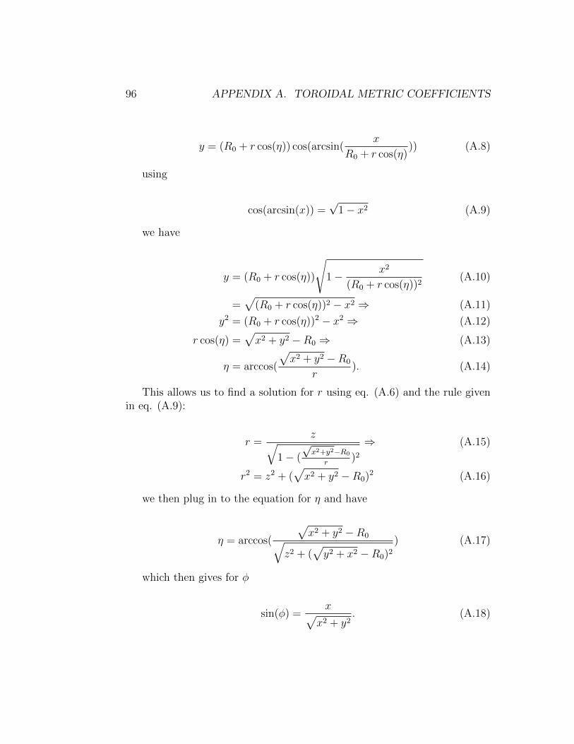
96 APPENDIX A. TOROIDAL METRIC COEFFICIENTS
y = (R0 + r cos(η)) cos(arcsin(x
R0 + r cos(η))) (A.8)
using
cos(arcsin(x)) =√
1− x2 (A.9)
we have
y = (R0 + r cos(η))
√1− x2
(R0 + r cos(η))2(A.10)
=√
(R0 + r cos(η))2 − x2 ⇒ (A.11)
y2 = (R0 + r cos(η))2 − x2 ⇒ (A.12)
r cos(η) =√x2 + y2 −R0 ⇒ (A.13)
η = arccos(
√x2 + y2 −R0
r). (A.14)
This allows us to find a solution for r using eq. (A.6) and the rule givenin eq. (A.9):
r =z√
1− (
√x2+y2−R0
r)2⇒ (A.15)
r2 = z2 + (√x2 + y2 −R0)
2 (A.16)
we then plug in to the equation for η and have
η = arccos(
√x2 + y2 −R0√
z2 + (√y2 + x2 −R0)2
) (A.17)
which then gives for φ
sin(φ) =x√
x2 + y2. (A.18)

97
We now find the gradient of the resulting expressions. Taking the gradienton both sides of r2 we have
2r∇r = 2zz +2(√x2 + y2 −R0)y√x2 + y2
y +2(√x2 + y2 −R0)x√x2 + y2
x (A.19)
Taking the gradient on both sides for cos(η) we have
− sin(η)∇η =xz2x+ yz2y + (
√x2 + y2 −R0)z
√x2 + y2z
(z2 + (√y2 + x2 −R0)2)
32
√x2 + y2
(A.20)
Finally taking the gradient on both sides of sin(φ) gives
cos(φ)∇φ =y2x+ xyy
(x2 + y2)32
(A.21)
The derived expressions allows us to derive the metric of the torusoidalgeometry. Using
gij = ∇ui · ∇uj (A.22)
we have
grr = ∇r · ∇r =z2
r2+
(y2 + x2)
r2
((√x2 + y2 −R0)
2
x2 + y2
)(A.23)
= sin2(η) +(R0 + r cos(η))2
r2
((r cos(η))2
(R0 + r cos(η))2
)= 1
and
gηη =1
sin2(η)
((x2 + y2)(z4 + (
√x2 + y2 −R0)
2z2)
(x2 + y2)(z2 + (√x2 + y2 −R0)2)3
)(A.24)
= r2(
1
(r2 sin2(η) + r2 cos2(η))2
)=
1
r2
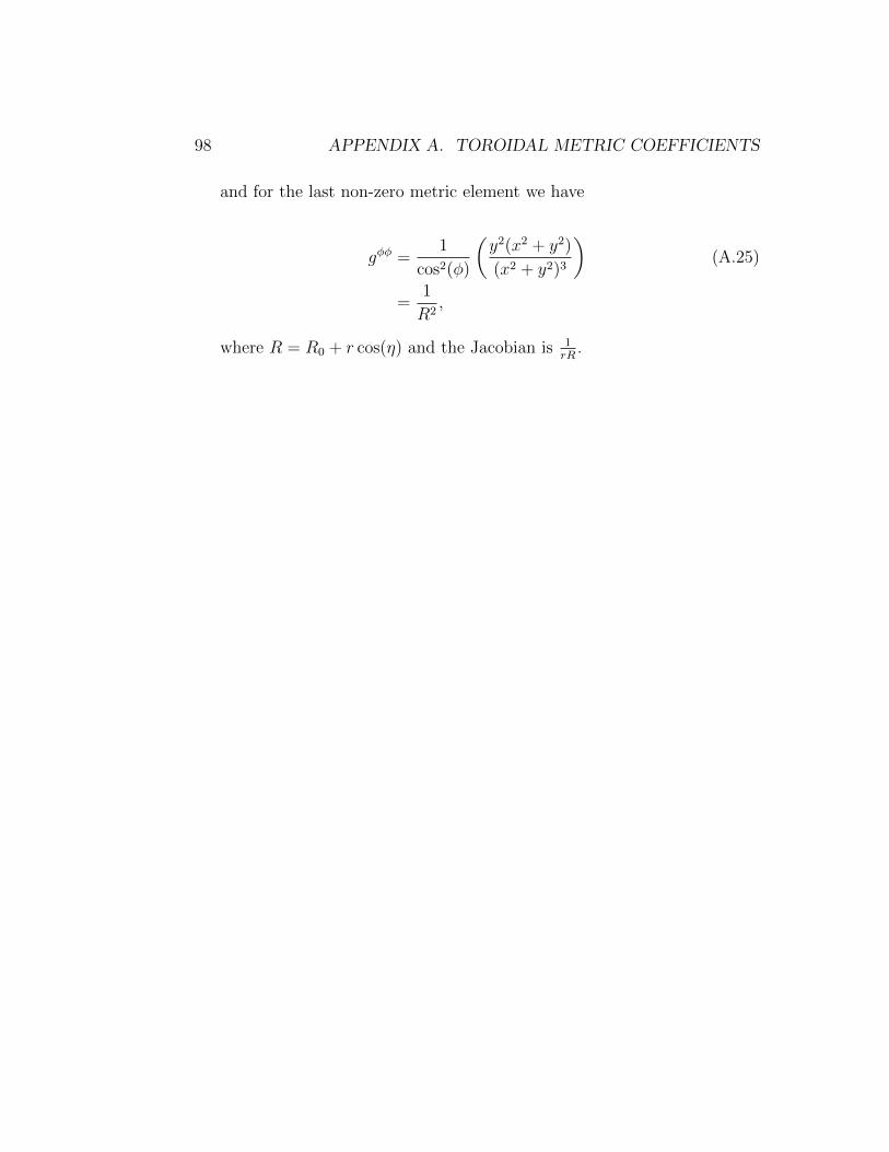
98 APPENDIX A. TOROIDAL METRIC COEFFICIENTS
and for the last non-zero metric element we have
gφφ =1
cos2(φ)
(y2(x2 + y2)
(x2 + y2)3
)(A.25)
=1
R2,
where R = R0 + r cos(η) and the Jacobian is 1rR
.
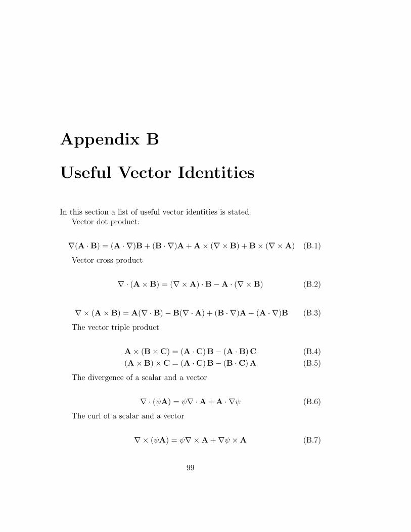
Appendix B
Useful Vector Identities
In this section a list of useful vector identities is stated.Vector dot product:
∇(A ·B) = (A · ∇)B + (B · ∇)A + A× (∇×B) + B× (∇×A) (B.1)
Vector cross product
∇ · (A×B) = (∇×A) ·B−A · (∇×B) (B.2)
∇× (A×B) = A(∇ ·B)−B(∇ ·A) + (B · ∇)A− (A · ∇)B (B.3)
The vector triple product
A× (B×C) = (A ·C) B− (A ·B) C (B.4)
(A×B)×C = (A ·C) B− (B ·C) A (B.5)
The divergence of a scalar and a vector
∇ · (ψA) = ψ∇ ·A + A · ∇ψ (B.6)
The curl of a scalar and a vector
∇× (ψA) = ψ∇×A +∇ψ ×A (B.7)
99

100 APPENDIX B. USEFUL VECTOR IDENTITIES

Bibliography
[1] J. Goldemberg, United Nations Development Programme, United Na-tions. Dept. of Economic, Social Affairs, and World Energy Council.World energy assessment: energy and the challenge of sustainability.United Nations Development Programme, 2000.
[2] K.S. Krane. Introductory Nuclear Physics. Wiley, 1987.
[3] M. P. Lucas, L. L. & Unterweger. Comprehensive review and criticalevaluation of the half-life of tritium. Journal of Research of the NationalInstitute of Standards and Technology, 105, 2000.
[4] J. Wesson and D.J. Campbell. Tokamaks. International Series of Mono-graphs on Physics. OUP Oxford, 2011.
[5] George M. Hornberger. New manuscript guidelines for the reportingof stable hydrogen, carbon, and oxygen isotope ratio data. Water Re-sources Research, 31(12):2895–2895, 1995.
[6] R. Fitzpatrick. Plasma Physics: An Introduction. Taylor & Francis,2014.
[7] Internal workings of a conventional tokamak with a centralsolenoid. credit: Max-planck institut fr plasmaphysik. http://www.
100milliondegrees.com/merging-compression/. Accessed: 2016-11-25.
[8] M.S. Tillack, A.D. Turnbull, C.E. Kessel, N. Asakura, A.M. Garofalo,C. Holland, F. Koch, Ch. Linsmeier, S. Lisgo, R. Maingi, R. Majeski,J. Menard, F. Najmabadi, R. Nygren, T.D. Rognlien, D.D. Ryutov, R.D.Stambaugh, P.C. Stangeby, and D.P. Stotler. Summary of the aries town
101
102 BIBLIOGRAPHY
meeting: edge plasma physics and plasma material interactions in thefusion power plant regime. Nuclear Fusion, 53(2):027003, 2013.
[9] P.M. Bellan. Fundamentals of Plasma Physics. Cambridge UniversityPress, 2008.
[10] W.D. D’haeseleer. Flux coordinates and magnetic field structure: a guideto a fundamental tool of plasma structure. Springer series in computa-tional physics. Springer-Verlag, 1991.
[11] P. Helander and D.J. Sigmar. Collisional Transport in Magnetized Plas-mas. Cambridge Monographs on Plasma Physics. Cambridge UniversityPress, 2005.
[12] B D Dudson, M V Umansky, X Q Xu, P B Snyder, and H R Wilson. Usermanual for BOUT++. Computer Physics Communications, 180:1467–1480, 2009.
[13] Tiago Ribeiro. Low frequency turbulence in the scrape-off layer of toka-mak plasmas. PhD thesis, Max Planck Institute for Plasma Physics,2006.
[14] B D Dudson, M V Umansky, X Q Xu, P B Snyder, and H R Wilson.BOUT++: A framework for parallel plasma fluid simulations. ComputerPhysics Communications, 180:1467–1480, 2009.
[15] Toroidal coordinates. http://fusionwiki.ciemat.es/fusionwiki/
images/1/10/Toroidal_coordinates.png. Accessed: 2016-11-25.
[16] Sren B Korsholm. Coherent structures and transport in drift waveplasma turbulence. PhD thesis, Technical University of Denmark, 2006.
[17] Akira Hasegawa and Masahiro Wakatani. Plasma edge turbulence. Phys.Rev. Lett., 50:682–686, Feb 1983.
[18] Hans L. Pecseli. Waves and Oscillations in Plasmas. Series in plasmaphysics. CRC Press, 2013.
[19] R.J. LeVeque. Finite Difference Methods for Ordinary and Partial Dif-ferential Equations: Steady-State and Time-Dependent Problems. SIAMe-books. Society for Industrial and Applied Mathematics (SIAM, 3600Market Street, Floor 6, Philadelphia, PA 19104), 2007.

BIBLIOGRAPHY 103
[20] Paul H. Rutherford and Edward A. Frieman. Stabilization of drift wavesby shear. Physics of Fluids, 10(5):1007–1016, 1967.