3D Simulation of Wind Turbine Rotors at Full Scale.Part I: Geometry Modeling and Aerodynamics

Y. Bazilevsa,∗, M.-C. Hsua, I. Akkermana, S. Wrightb, K. Takizawab, B. Henickeb,T. Spielmanb, T.E. Tezduyarb

aDepartment of Structural Engineering, University of California, San Diego, 9500 Gilman Drive,La Jolla, CA 92093, USA

bMechanical Engineering, Rice University - MS 321, 6100 Main Street, Houston, TX 77005, USA

Abstract

In this two-part article we present a collection of numerical methods combined intoa single framework, which has the potential for a successful application to windturbine rotor modeling and simulation. In Part 1 of this article we focus on: 1.The basics of geometry modeling and analysis-suitable geometry construction forwind turbine rotors; 2. The fluid mechanics formulation and its suitability andaccuracy for rotating turbulent flows; 3. The coupling of air flow and a rotatingrigid body. In Part 2 we focus on the structural discretization for wind turbineblades and the details of the fluid–structure interaction computational procedures.The methods developed are applied to the simulation of the NREL 5MW offshorebaseline wind turbine rotor. The simulations are performed at realistic wind velocityand rotor speed conditions and at full spatial scale. Validation against published datais presented and possibilities of the newly developed computational framework areillustrated on several examples.

Keywords: wind turbine rotor, wind turbine blades, fluid–structure interaction,geometry modeling, isogeometric analysis, NURBS, rotating turbulent flow,aerodynamic torque

1. Introduction

Countries in Europe and Asia are putting substantial effort behind the develop-ment of wind energy technologies. Currently in the EU, 50 GW of electricity comesfrom the on-land and 1 GW from offshore wind turbines. The EU target is to raisethe on-land production to 130 GW and offshore to 50 GW by 2020. The latter fig-ure represents a fifty-fold increase, which will require a significant investment andengineering effort. The US Government recently established the objective that wind

∗Corresponding authorEmail address: yuri@ucsd.edu (Y. Bazilevs)

Preprint submitted to International Journal for Numerical Methods in Fluids September 2, 2014

power should supply 25% of the US energy needs by 2025. Achieving this objec-tive will require nearly a 1200% increase in wind power capacity (from 25 GW to305 GW). We believe that in order to achieve this goal, the US must also investsignificant resources in the development of offshore wind turbines. We also believethat leading-edge wind energy research and development, which includes advancedsimulation, will be essential in meeting this goal.

The present cost for wind energy is nonetheless strongly dominated by risingoperations and maintenance costs over the current 20-year design lifetime of thesystem [1]. Although the design lifetime is 20 years, a typical wind turbine fails2.6 times during the first 10 years, usually within the gearbox, generator and ro-tor assembly, and the rotor assembly has been identified as the top opportunity formajor advancement in design and performance improvements [2]. While wind tur-bine rotor failures occur due to a variety of reasons, fatigue failure of the windturbine blades due to their everyday operation is recognized as one of the majorcauses. However, the industry is currently unable to predict these failure mecha-nisms, which leads to the unscheduled downtime, expensive maintenance and re-duced capacity.

In offshore environments the winds are typically stronger and are more sus-tained than inland, providing a more reliable source of energy. This in part explainsthe attraction to offshore designs. However, offshore wind turbines are exposed toharsh environments and must be designed to reliably sustain increased wind loads.Increased wind speeds also imply that the blades of much larger diameter (120 m– 190 m) must be designed and built for better performance. These are signifi-cant engineering challenges that must be addressed through advanced research anddevelopment, which also involves large-scale advanced simulation.

The current practice in wind turbine simulation makes use of steady (time-independent), 2D lumped-parameter aerodynamic models for airfoil cross-sectionsthat are coupled with 1D beam-type structures to evaluate wind turbine blade de-signs and, specifically, their aerodynamic performance. These models are simpleto implement and fast to execute, which makes them attractive for industrial appli-cations, especially if they are routinely used as part of the design cycle. However,due to the steady nature of the flow conditions and the lack of real 3D geometry andphysics, these models are unable to adequately represent the system response totime-dependent phenomena, such as wind gusts, or phenomena attributable to com-plex blade geometry and material composition, such as flow separation and reat-tachment and detailed blade deformations and stress distributions. It is preciselythese more extreme events that cause gearbox and blade failures and significantlyreduce the life cycle of wind turbines, leading to premature maintenance and repairand, as a result, to increased cost of wind energy. A more fundamental problem withthese simple models is their non-hierarchical nature: it is virtually not possible toenhance them with features necessary for predicting more extreme events or richerphysics without going to a more advanced modeling framework all together.

In this work we propose to introduce a paradigm shift in wind turbine model-

2

ing and simulation by developing 3D, complex geometry, time-dependent, multi-physics modeling procedures for wind turbine fluid–structure interaction (FSI). Inparticular, we focus on predicting wind turbine blade–air flow interaction phenom-ena for real wind turbines, operating under real wind conditions, and at full designscale. The particular focus on turbine blades is motivated by the fact that improvedblade efficiency directly translates to lower cost of wind energy conversion. How-ever, full-scale 3D FSI simulations of wind turbines engender a set of challenges.The air flow Reynolds number is on the order of 107 − 108, which is challengingin terms of both flow modeling and simulation. This Reynolds number necessitatesthe use of fine grids, good quality basis functions, and large-scale high-performancecomputing. Wind turbine blades are long and slender structures that are made ofseveral structural components with complex distribution of material properties, re-quiring both advanced computational model generation and simulation methods.The numerical approach for structural mechanics must have good accuracy andavoid locking. The latter is typical of thin structures [3]. Wind turbine bladesare manufactured using multi-layer composite materials that also require appropri-ate numerical treatment. The numerical simulations simultaneously involve movingand stationary components, which must be handled correctly. The fluid–structurecoupling must be efficient and robust to preclude divergence of the computations.Some of these challenges will be addressed in this work.

Isogeometric Analysis, first introduced in [4] and further expanded on in [5–16],is adopted as the geometry modeling and simulation framework for wind turbines.It is particularly well suited for this application for the following reasons. We useNURBS (non-uniform rational B-splines), the most developed basis function tech-nology for isogeometric analysis. NURBS are more efficient than standard finiteelements for representing complex, smooth geometrical shapes, such as wind tur-bine blades. Because the geometry and solution fields are represented using thesame functional description, the integration of geometry modeling with structuraldesign and computational analysis is greatly simplified. Isogeometric analysis wassuccessfully employed for computation of turbulent flows [17–22], nonlinear struc-tures [23–28] and FSI [29–32]. In most cases, isogeometric analysis gave a clear ad-vantage over standard low-order finite elements in terms of solution per-degree-of-freedom accuracy, which is in part attributable to the higher-order smoothness of thebasis functions employed. Flows about rotating components are naturally handledin an isogeometric framework because all conic sections, and, in particular, circularand cylindrical shapes are represented exactly [33]. In addition, an isogeometricrepresentation of the analysis-suitable geometry may be used to construct tetrahe-dral and hexahedral meshes for computations using finite elements. In this paper,we use such tetrahedral meshes for wind turbine computation with the Deforming-Spatial-Domain/Stabilized Space–Time (DSD/SST) formulation [34–38].

The DSD/SST formulation was introduced in [34–36] as a general-purposeinterface-tracking (moving-mesh) technique for flow computations involving mov-ing boundaries and interfaces, including FSI and flows with moving mechani-

3

cal components. Some of earliest FSI computations with the DSD/SST formula-tion were reported in [39] for vortex-induced vibrations of a cylinder and in [40]for flow-induced vibrations of a flexible, cantilevered pipe (1D structure with 3Dflow). The DSD/SST formulation has been used extensively in 3D computations ofparachute FSI, starting with the 3D computations reported in [41–43] and evolvingto computations with direct coupling [44, 45]. New versions of the DSD/SST for-mulation introduced in [38] are the core technologies of the stabilized space–timeFSI (SSTFSI) technique, which was also introduced in [38]. The SSTFSI technique,combined with a number of special techniques [38, 46–56], have been used in someof the most challenging parachute FSI computations [48, 51, 54, 56, 57], and alsoin a good number of patient-specific arterial FSI computations [50, 52, 53, 55]. Inapplication of the DSD/SST formulation to flows with moving mechanical com-ponents, the Shear–Slip Mesh Update Method (SSMUM) [58–60] has been veryinstrumental. The SSMUM was first introduced for computation of flow aroundtwo high-speed trains passing each other in a tunnel (see [58]). The challenge wasto accurately and efficiently update the meshes used in computations based on theDSD/SST formulation and involving two objects in fast, linear relative motion. Theidea behind the SSMUM was to restrict the mesh moving and remeshing to a thinlayer of elements between the objects in relative motion. The mesh update at eachtime step can be accomplished by a “shear” deformation of the elements in thislayer, followed by a “slip” in node connectivities. The slip in the node connectivi-ties, to an extent, un-does the deformation of the elements and results in elementswith better shapes than those that were shear-deformed. Because the remeshingconsists of simply re-defining the node connectivities, both the projection errorsand the mesh generation cost are minimized. A few years after the high-speed traincomputations, the SSMUM was implemented for objects in fast, rotational relativemotion and applied to computation of flow past a rotating propeller [59] and flowaround a helicopter with its rotor in motion [60].

Part 1 of this paper, which focuses on geometry modeling and aerodynamics ofwind turbines, is outlined as follows. In Section 2, we describe a template-basedmethod for creating an analysis-suitable NURBS geometry for FSI simulation ofwind turbine rotors. We apply the method developed to construct the NREL 5MWoffshore baseline wind turbine rotor given in [61]. In Section 3, we develop theresidual-based variational multiscale formulation of the Navier–Stokes equationsof incompressible flow on a moving domain. We develop a generalization of thequasi-static fine scale assumption to the moving domain case, which leads to a semi-discrete formulation that globally conserves linear momentum. In Section 4, weperform a partial validation of the proposed computational method on a turbulentTaylor–Couette flow. In Section 5, we formulate a coupled problem, which involvesincompressible flow with a rigidly rotating body. Rotationally-periodic boundaryconditions, which allow us to take advantage of the problem symmetry for bettercomputational efficiency, are also described. To assess the accuracy of the numericalmethod, the NREL 5MW offshore baseline wind turbine rotor is simulated using

4

prescribed inflow wind conditions and rotor speed. The NURBS-based simulationresults compare favorably to the reference data from [61]. A coupled simulation forthe case of high inflow wind speed and free rotation, which corresponds to the caseof rotor over-spinning in the case of the control system failure, is also performed toillustrate the possibilities of the proposed computational procedures. In Section 6,we draw conclusions and outline future research directions.

2. Analysis-Suitable Geometry Construction for Wind Turbine Rotors

We propose a template-based wind turbine geometry modeling approach thatmakes use of volumetric NURBS. The method entails construction of one or more(small number of) template geometries of wind turbine designs. The templates in-clude and closely approximate the geometry of the rotor blades and hub (nacelle),and the flow domain around. The template geometry is then deformed to the actualgeometry of the wind turbine by appropriately minimizing the error between them.Once the model is generated, an analysis-ready geometry is produced with usercontrol over mesh refinement and domain partitioning for efficient parallel process-ing. The advantage of this approach is that it can be specialized and optimized fora particular class of geometries. For example, a template-based geometry modelingapproach was developed and successfully employed for NURBS modeling and FSIsimulation of vascular blood flow with patient-specific data in [29].

2.1. Wind turbine rotor blade and hub geometry construction

x/c

y/c

0 0.2 0.4 0.6 0.8 1

-0.2

-0.1

0

0.1

0.2

DU40DU35DU30DU25DU21NACA64

Figure 1: Airfoil cross-sections used in the design of the wind turbine rotor blades.

As a first step we construct a template for the structural model of the rotor.In this paper, the structural model is limited to a surface (shell) representation ofthe wind turbine blade, the hub, and their attachment zone. The blade surface isassumed to be composed of a collection of airfoil shapes that are lofted in the blade

5

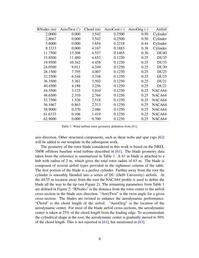
RNodes (m) AeroTwst () Chord (m) AeroCent (-) AeroOrig (-) Airfoil2.0000 0.000 3.542 0.2500 0.50 Cylinder2.8667 0.000 3.542 0.2500 0.50 Cylinder5.6000 0.000 3.854 0.2218 0.44 Cylinder8.3333 0.000 4.167 0.1883 0.38 Cylinder

11.7500 13.308 4.557 0.1465 0.30 DU4015.8500 11.480 4.652 0.1250 0.25 DU3519.9500 10.162 4.458 0.1250 0.25 DU3524.0500 9.011 4.249 0.1250 0.25 DU3028.1500 7.795 4.007 0.1250 0.25 DU2532.2500 6.544 3.748 0.1250 0.25 DU2536.3500 5.361 3.502 0.1250 0.25 DU2140.4500 4.188 3.256 0.1250 0.25 DU2144.5500 3.125 3.010 0.1250 0.25 NACA6448.6500 2.310 2.764 0.1250 0.25 NACA6452.7500 1.526 2.518 0.1250 0.25 NACA6456.1667 0.863 2.313 0.1250 0.25 NACA6458.9000 0.370 2.086 0.1250 0.25 NACA6461.6333 0.106 1.419 0.1250 0.25 NACA6462.9000 0.000 0.700 0.1250 0.25 NACA64

Table 1: Wind turbine rotor geometry definition from [61].

axis direction. Other structural components, such as shear webs and spar caps [62]will be added to our template in the subsequent work.

The geometry of the rotor blade considered in this work is based on the NREL5MW offshore baseline wind turbine described in [61]. The blade geometry datataken from the reference is summarized in Table 1. A 61 m blade is attached to ahub with radius of 2 m, which gives the total rotor radius of 63 m. The blade iscomposed of several airfoil types provided in the rightmost column of the table.The first portion of the blade is a perfect cylinder. Further away from the root thecylinder is smoothly blended into a series of DU (Delft University) airfoils. Atthe 44.55 m location away from the root the NACA64 profile is used to define theblade all the way to the tip (see Figure 2). The remaining parameters from Table 1are defined in Figure 2: “RNodes” is the distance from the rotor center to the airfoilcross-section in the blade axis direction. “AeroTwst” is the twist angle for a givencross-section. The blades are twisted to enhance the aerodynamic performance.“Chord” is the chord length of the airfoil. “AeroOrig” is the location of theaerodynamic center. For most of the blade airfoil cross-sections, the aerodynamiccenter is taken at 25% of the chord length from the leading edge. To accommodatethe cylindrical shape at the root, the aerodynamic center is gradually moved to 50%of the chord length. This is not reported in [61], but mentioned in [63].

6

Figure 2: Illustration of quantities from Table 1.

Remark: There is some redundancy in the parameters given in Table 1. Thevariable “AeroCent” is used as an input to FAST [64], which is the aerodynamicsmodeling software that is typically used for wind turbine rotor computations. FASTis based on look-up tables and provides blade cross-section steady-state lift anddrag forces given the airfoil type, relative wind speed, and angle of attack. Theeffects of the hub, trailing edge turbulence, and blade tip are modeled using em-pirical relationships. FAST assumes that the blade-pitch axis passes through eachairfoil section at 25% chord length, and defines AeroCent−0.25 to be the fractionaldistance to the aerodynamic center from the blade-pitch axis along the chordline,positive toward the trailing edge. Therefore, AeroOrig + (0.25 − AeroCent) givesthe location of where the blade-pitch axis passes through each airfoil cross-section.Although for our purposes this added complexity is unnecessary, the same namingsystem is used for backward compatibility with the reference reports.

For each blade cross-section we use quadratic NURBS to represent the 2D air-foil shape. The weights of the NURBS functions are set to unity. The weightsare adjusted near the root to represent the circular cross-sections of the blade ex-actly. The cross-sections are lofted in the blade axis direction, also using quadraticNURBS and unity weights. This geometry modeling procedure produces a smoothrotor blade surface using a relatively small number of input parameters, which isan advantage of the isogeometric representation. The final shape of the blade alongwith the airfoil cross-sections is shown in Figure 3a. Figure 3b shows a top view ofthe blade in which the twisting of the cross-sections is evident.

2.2. Volumetric NURBSGiven the rotor blade surface description, the surrounding fluid domain volume

is constructed next. The blade surface is split into four patches of similar size, whichwe call the blade surface patches. The splitting is done at the leading and trailing

7

(a)

(b)

Figure 3: (a) Airfloil cross-sections superposed on the wind turbine blade. (b) Top view of a subsetof the airfoil cross-sections illustrating blade twisting.

edges, as well as half-way in between on both sides of the blade. The volumetricfluid domain near the blade is generated for each one of the blade surface patches.As a final step, the fluid domain patches are merged such that the outer boundary ofthe fluid domain is a perfect cylinder.

For each of the blade surface patches we create a 60 pie-shaped domain using aminimum required number of control points. The control points at the bottom of thepatch are moved to accommodate the shape of the rotor hub (see Figure 4a). As anext step, we perform knot insertion and move the new control points such that theirlocations coincide with those of the blade surface patch. See Figure 4b and Figure4c for knot insertion and control point re-positioning, respectively. This generatesan a-priori conforming discretization between the volumetric fluid domain and thesurface of the structural model, suitable for FSI analysis. Finally, the fluid domainis refined in all parametric directions for analysis. Figure 4d shows the rotor surface

8

mesh and one of the fluid mesh subdomains adjacent to it. The remaining fluidsubdomains are generated in the same manner.

The resultant fluid NURBS mesh may be embedded into a larger domain forthe purposes of simulation. In this work we take this larger domain to also be acylinder. For computational efficiency, only one-third of the domain is modeled.The fluid volume mesh, corresponding to one-third of the fluid domain, consists of1,449,000 quadratic NURBS elements (and a similar number of control points) andis shown in Figure 5a. The fluid mesh cross-section that also shows the details ofmesh refinement in the boundary layer is shown in Figure 5b. The wind turbinerotor surface model and outer cylindrical domain of the three-blade configurationare shown in Figure 6. Mesh refinement was concentrated near the wind turbineblade surface. No special attention was paid to mesh design in the outer regions ofthe computational domain.

Remark: We note that the template-based nature of the proposed approachand a relatively small number of input parameters for model building allow one toalter the wind turbine rotor models with minimal effort.

3. Navier–Stokes Equations of Incompressible Flow and Residual-Based Tur-bulence Modeling for Moving Domains

3.1. The weak formulationIn what follows, Ω ⊂ Rd, d = 2, 3 denotes the spatial domain occupied by the

fluid at the current time and Γ = ∂Ω is its boundary. Let V and W denote theinfinite-dimensional trial solution and weighting function spaces, respectively, andlet (·, ·)Ω denote the L2-inner product over Ω. The weak form of the Navier–Stokesequations of incompressible flow over a moving domain is stated as follows: findthe velocity-pressure pair v, p ∈ V such that for all momentum and continuityweighting functions w, q ∈ W,

B(w, q, v, p) − (w, ρ f )Ω = 0, (1)

where

B(w, q, v, p) =

(w, ρ

∂v∂t

)Ω

+ (w, ρ(v − v) · ∇v)Ω + (q,∇ · v)Ω

− (∇ · w, p)Ω + (∇sw, 2µ∇sv)Ω . (2)

In the above, v is the fluid domain velocity, µ is the kinematic viscosity, ρ is thedensity, and

∇sv =12

(∇v + ∇vT ) (3)

9

is the symmetric gradient of the particle velocity field. Equation (1) is a weakform corresponding to the Arbitrary Lagrangian–Eulerian (ALE) formulation of theNavier–Stokes equations and the time derivative in the first term on the right-hand-side of Eq. (2) is taken with respect to a fixed spatial coordinate in the referenceconfiguration. In the absence of the fluid domain motion, the above formulationreverts to a standard incompressible flow formulation on a stationary domain.

Direct replacement of the infinite-dimensional spaces V andW by their finitedimensional counterparts leads to the Galerkin formulation, which is unstable foradvection-dominated flow and for the choice of equal-order velocity–pressure dis-cretization. In what follows, we make use of the variational multiscale method (see,e.g., [65, 66]) to generate a stable and accurate discrete formulation over a movingdomain that is suitable for equal-order velocity–pressure discretization.

3.2. Residual-based variational multiscale (RBVMS) formulation of flow over amoving domain

Following the developments in [17], the trial solution and weighting functionspaces are split into coarse and fine scales as

v, p =vh, ph + v′, p′, (4)

w, q =wh, qh + w′, q′. (5)

In the above, the superscript h denotes resolved coarse scales represented by the fi-nite element or isogeometric discretization. The primed quantities correspond to theunresolved scales and will be modeled. The above decomposition of the weightingfunctions leads to two variational sub-problems:

B(wh, qh, vh, ph + v′, p′) − (wh, ρ f )Ω =0, ∀wh, qh ∈ Wh, (6)

B(w′, q′, vh, ph + v′, p′) − (w′, ρ f )Ω =0, ∀w′, q′ ∈ W′, (7)

where Wh is the finite-dimensional space of finite element or isogeometric func-tions and W′ is an infinite dimensional space of the unresolved fine scales. Weproceed as in [17] and model the fine-scale velocity and pressure as being propor-tional to the strong form of the Navier–Stokes partial differential equation residual

v′ = −τM rM(vh, ph), (8)

p′ = −τCrC(vh), (9)

rM(v, p) = ρ∂v∂t

+ ρ(v − v) · ∇v + ∇p − µ∆v − ρ f , (10)

rC(v) = ∇ · v. (11)

The parameters τM and τC in the above equations originate from stabilized finiteelement methods for fluid dynamics (see, e.g., [34, 37, 67–74]) and are referredto as stabilization parameters. Recently, they were interpreted as the appropriate

10

averages of the small-scale Green’s function, which is a key mathematical objectin the theory of variational multiscale methods (see [75] for an elaboration). Wenote that in this paper the stabilization parameters are defined in a form where theyhave the units of time divided by density, instead of the units of time, which is moretypical.

To generate the numerical method, v′ and p′ in Eqs. (8) and (9) are inserted di-rectly into the coarse-scale equations given by Eq. (6). To simplify the formulation,two assumptions are typically employed: 1) the fine scales are orthogonal to thecoarse scales with respect to the inner-product generated by the viscous term; and2) the fine scales are quasi-static. The latter condition is expressed as

∂v′

∂t= 0. (12)

In this work, we would like to illustrate that the quasi-static assumption on the finescales takes on a different form in the case of a moving fluid domain. In particular,we postulate the following generalized quasi-static condition on the fine scales

∂Jv′

∂t= 0, (13)

where J is the determinant Jacobian of the mapping from the referential to the spa-tial domain in the ALE framework (see, e.g., [31]), and the time derivative is takenwith respect to the fixed referential coordinate. Differentiating the product and re-arranging terms, gives

∂v′

∂t= −(∇ · v)v′. (14)

Note that in the case of divergence-free fluid domain motions (e.g., stationary orrotating domains), the above definition reverts to the original quasi-static subgridscale assumption.

Examining the influence of the fine scales in the time derivative and convectiveterms, we obtain(

wh, ρ∂(vh + v′)

∂t

)Ω

=

(wh, ρ

∂vh

∂t

)Ω

−(wh, ρ(∇ · v)v′

)Ω, (15)

and (wh, ρ(vh + v′ − v) · ∇(vh + v′)

)Ω

=(wh, ρ(vh + v′ − v) · ∇vh

)Ω

−(∇wh, ρv′ ⊗ (vh + v′ − v)

)Ω

−(wh, ρ∇ · (vh + v′ − v)v′

)Ω, (16)

11

respectively. Assuming incompressibility of the particle velocity field (i.e., ∇ · (vh +

v′) = 0) and rearranging the terms in Eq. (16), we obtain(wh, ρ(vh + v′ − v) · ∇(vh + v′)

)Ω

=(wh, ρ(vh − v) · ∇vh

)Ω

−(∇wh, ρv′ ⊗ (vh − v)

)Ω

+(wh, ρv′ · ∇vh

)Ω

−(∇wh, ρv′ ⊗ v′

)Ω

+(wh, ρ(∇ · v)v′

)Ω. (17)

The above development leads to the following semi-discrete variational formu-lation: find vh, ph ∈ Vh, vh = g on Γg, such that ∀wh, qh ∈ Vh, wh = 0 on Γg,

B(wh, qh, vh, ph) + Bvms(wh, qh, vh, ph) − (wh, ρ f )Ω = 0, (18)

where the modeled subgrid-scale terms in Bvms are

Bvms(w, q, v, p) = (∇w, ρτM rM(v, p) ⊗ (v − v))Ω

+ (∇ · w, τC∇ · v)Ω

− (w, ρτM rM(v, p) · ∇v)Ω

− (∇w, ρτM rM(v, p) ⊗ τM rM(v, p))Ω

+ (∇q, τM rM(v, p))Ω , (19)

and the integrals are taken element-wise.

Remark: Comparing Eqs. (15) and (17) we note that the last term on theright-hand-side of Eq. (17) cancels that of Eq. (15). This leads to the discreteformulation given by Eq. (18) that globally conserves linear momentum (see [31]for a derivation). This would not be the case if the quasi-static assumption given byEq. (12) is employed.

Remark: The above discrete formulation may be augmented with weakly-enforced Dirichlet boundary conditions [76] to enhance solution accuracy in thepresence of unresolved boundary layers.

Remark: A similar approach for deriving the multiscale formulation of theNavier–Stokes equations on a moving domain was presented in [77]. However, aquasi-static fine scale assumption given by Eq. (12) was used instead of Eq. (14).

4. Application to Turbulent Rotating Flow: Taylor–Couette Flow at Re = 8000

We simulate the turbulent Taylor–Couette flow, which is a flow between twoconcentric cylinders. We feel that this test case is relevant to wind turbines, because

12

the flow exhibits several complex features in common with the present application,such as rotation, curved walls, boundary layers, and highly complex time-dependentevolution of the velocity and pressure fields, all of which are challenging to com-pute. At the same time, much is known about this problem experimentally (see,e.g., [78]), and numerically (see, e.g., [22, 79–83]), which makes this test case avery good candidate for verification and validation of numerical formulations forturbulent fluid flow.

One of the bigger challenges involved in simulation of rotating turbulent flowis turbulence modeling. Eddy-viscosity models rely on the continuous energy cas-cade, i.e., the continuous energy transfer from low to high modes in the turbulentflow (see, e.g., [84]). However, as explained in [85], in the presence of high ro-tation rates the energy cascade is arrested. This renders most well-accepted eddy-viscosity models inconsistent in the rotation dominated regime. The advantage ofthe present turbulence modeling approach is that the unresolved scales are modeledusing the variational multiscale methodology, and the explicit use of eddy viscosi-ties is avoided all together. As a result, the present approach is not likely to sufferfrom the shortcomings of eddy-viscosity-based turbulence models for flows withhigh rotation rates.

The problem setup is as follows. The inner cylinder rotates at a constant angularvelocity, while the outer cylinder is stationary (see Figure 7a). Periodic boundaryconditions are imposed in the axial direction, and no-slip boundary conditions areapplied at the cylinder surfaces. The no-slip conditions are imposed weakly usingthe methodology presented in [19]. The Reynolds number of the flow based onthe speed of the inner cylinder and the gap between the cylinders is Re = Uθ(R1 −

R0)ρ/µ = 8000. The fluid density is set to ρ = 1, the dynamic viscosity is set toµ = 1/8000, the inner and outer radii are set to R0 = 1 and R1 = 2, respectively, andthe inner cylinder wall speed is set to Uθ = 1. Due to the rotational symmetry ofthe problem geometry, the simulations are performed over a stationary domain. Theresults of our simulation are compared with the DNS of [86], where this test casewas computed using 256 Fourier modes in the axial direction and 400 9th-orderspectral finite elements in the remaining directions. This is the highest Reynoldsnumber DNS available for this flow. For an overview of spectral finite elementsapplied to fluid dynamics, see, for example, [87].

We solve the problem on meshes consisting of linear finite elements andquadratic NURBS. The quadratic NURBS give exact representation of the geome-try, while linear FEM only approximates it. However, the geometry approximationimproves with refinement. We deliberately sacrifice the boundary layer resolutionby using uniform meshes in all directions, including the wall-normal. Our goal isto see the performance of the proposed method in the case of unresolved bound-ary layers and rotational dominance, as well as to assess the accuracy benefits ofthe NURBS-based approach relative to standard FEM for this challenging situation.We note that two of the authors have successfully computed this test case usingquadratic NURBS with boundary layer refinement in [22].

13

The simulation is started using a linear laminar profile of the azimuthal velocity.After transition to turbulence, the flow is advanced in time until the solution reachesa statistically-stationary state. Figure 7b shows the isosurfaces of a scalar quantityQ, which is defined as

Q = Ω : Ω − ∇svh : ∇svh, (20)

where Ω = 12 (∇vh − ∇vhT ) is the skew-symmetric part of the velocity gradient. Q is

designed to be an objective quantity for identifying vortical features in the turbulentflow (see, e.g., [88]). The figure illustrates the complexity of the turbulent flow andthe high demand on the numerical method to adequately represent it.

Flow statistics are given in the form of mean azimuthal velocity and angularmomentum, both as functions of the radial coordinate. The velocity data is collectedat mesh knots, rotated to the cylindrical coordinate system, and ensemble-averagedover the periodic directions and time.

Figure 8 shows mean azimuthal velocity results and compares linear FEM andquadratic NURBS. Linear elements give a reasonable approximation of the meanflow, especially considering the few degrees of freedom employed and no bound-ary layer resolution. The quadratic NURBS, which use nearly the same numberof degrees of freedom as linear elements, produces results of remarkable accuracy.Even with the coarse mesh, for which the boundary layer lies completely within thefirst element in the wall-normal direction, the mean velocity curve nearly interpo-lates the DNS. The same conclusions hold for the mean angular momentum resultsshown in Figure 9.

This problem illustrates that the variational multiscale method in conjunctionwith NURBS-based isogeometric analysis can deliver very accurate results for ro-tating turbulent flow. In what follows, we apply the proposed method to wind tur-bine simulation. We are cognizant of the fact that the Reynolds number in the caseof wind turbines is orders of magnitude higher than for the test case consideredin this section. Hence, the results presented in this section constitute only partialvalidation of the proposed computational method.

5. Wind Turbine Simulations

5.1. Coupling of a rigid rotor with incompressible flowIn this section we present the formulation of the coupled problem that involves

incompressible fluid and a rigid body that undergoes rotational motion. We spe-cialize the formulation to the case of a wind turbine rotor whose axis of rotationcoincides with the z-direction. We denote by θ the angle of rotation of the windturbine rotor about the z-axis from the reference configuration. The rotor angularvelocity and acceleration are found by differentiating θ with respect to time, and aredenoted by θ and θ, respectively. The coupled problem amounts to finding the triple

14

vh, ph, θ such that for all test functions wh, qh

B(wh, qh, vh, ph) + Bvms(wh, qh, vh, ph) − (wh, ρ f )Ω = 0, (21)

Iθ + f (θ, t) − T f (vh, ph) = 0, (22)

where I is the rotor moment of inertia, f (θ, t) may represent forcing due to frictionin the system or interaction with the generator, and T f (vh, ph) is the torque exertedon the rotor by the fluid, i.e. the aerodynamic torque. This is a two-way coupledproblem: the fluid solution depends on the rotor position and speed, while the rotorequation is driven by the fluid torque.

The fluid domain rotates with the same angular speed as the rotor. This meansthe fluid domain current configuration is defined as

Ω = x | x = R(θ)[X − X0] + X0, X ∈ Ω0, (23)

where Ω0 is the fluid domain in the reference configuration, X0 is the rotor centerof mass, and R(θ) is the rotation matrix given by

R(θ) =

cos θ − sin θ 0sin θ cos θ 0

0 0 1

. (24)

With the above definition of the fluid domain motion, the fluid domain velocitybecomes

v =dR(θ)

dθ[X − X0] θ. (25)

The aerodynamic torque is given by

T f (v, p) =

∫Γrot

r × (pn− 2µ∇sv · n)dΓ, (26)

where Γrot is the rotor surface, r = x−x0 is the radius-vector from the rotor center ofmass in the current configuration, and n is the unit normal to the rotor surface. In thecomputations, instead of using Eq. (26) directly, we opt for a conservative definitionof the aerodynamic torque. For this, we first define the discrete momentum equationresidual at every finite element node or isogeometric control point A and cartesiandirection i as

RA,i = B(NAei, 0, vh, ph) + Bvms(NAei, 0, vh, ph) − (NAei, ρ f )Ω, (27)

where NA’s are the velocity basis functions and ei’s are the Cartesian basis vectors.The residual RA,i vanishes everywhere in the domain except at the rotor surfacecontrol points (or nodes). The conservative aerodynamic torque along the z-axis

15

may now be computed as

T f (vh, ph) =∑A, j,k

ε3 jkrA, jRA,k, (28)

where εi jk’s are the cartesian components of the alternator tensor and rA, j are thenodal or control point coordinates.

The coupled system given by Eqs. (21)–(22) is advanced in time using theGeneralized-alpha method (see [31, 89, 90]) for both the fluid and rotor equations.Within each time step, the coupled equations are solved using an inexact Newtonapproach. For every Newton iteration we obtain the fluid solution increment,update the fluid solution, compute the aerodynamic torque, obtain the rotorsolution increment, and update the rotor solution and the fluid domain velocity andposition. The iteration is repeated until convergence. Because the wind turbinerotor is a relatively heavy structure, the proposed approach, also referred to as“block-iterative” (see [44] for the terminology), is stable.

Remark: The case of prescribed angular velocity is also of interest and canbe obtained by providing a time history of θ, which obviates Eq. (22). We makeuse of this in the sequel, where we perform a validation study of our wind turbinerotor configuration.

Remark: We note that the torque definition given by Eq. (28) makes use ofthe isoparametric property of the finite element and isogeometric methods. Besidesthe possible accuracy benefits associated with a conservative definition of torque,the formulation avoids performing boundary integration and makes use of thesame “right-hand-side” routine as the fluid assembly itself, which simplifiesimplementation.

Remark: The conservative torque definition given by Eq. (28) is only appli-cable for strongly enforced velocity boundary conditions, which are employed inthis work for wind turbine simulations. For the case of weak boundary conditions,a conservative definition of the torque given in [22] may be used instead.

5.2. Rotationally-periodic boundary conditionsTo enhance the efficiency of the simulations, we take advantage of the problem

rotational symmetry and only construct a 120 slice of the computational domain(see Section 2). However, to carry out the simulations, rotationally-periodic bound-ary conditions must be imposed. Denoting by vl and vr the fluid velocities at the leftand right boundary, respectively (see Figure 10), and by pl and pr the correspondingpressures, we set

pl = pr, (29)vl = R(2/3π) vr. (30)

16

That is, while the pressure degrees-of-freedom take on the same values, the fluidvelocity degrees-of-freedom are related through a linear transformation with therotation matrix from Eq. (24) evaluated at θ = 2/3π. Note that the transformationmatrix is independent of the current domain position.

Rotationally periodic boundary conditions are implemented through standardmaster-slave relationships. During the discrete residual assembly (see Eq. (27)), thenodal or control-point momentum residual at the slave boundary is rotated usingRT (2/3π) and added to the master residual (assumed to reside at the right bound-ary). Once the fluid solution update is computed, the velocity solution at the masterboundary is rotated using R(2/3π) prior to communicating it to the slave bound-ary. All of the numerical examples presented in this article use rotationally-periodicboundary conditions. We note that rotationally periodic boundary conditions wereemployed earlier in [54, 56, 91] for parachute simulations.

5.3. Simulations with prescribed rotor speed: A validation studyWe compute the aerodynamics of the NREL 5MW offshore baseline wind tur-

bine [61] with prescribed rotor shape and speed with a rotating mesh. The rotorradius, R, is 63 m. The wind speed is uniform at 9 m/s and the rotor speed is1.08 rad/s, giving a tip speed ratio of 7.55 (see [92] for wind turbine terminology).We use air properties at standard sea-level conditions. The Reynolds number (basedon the cord length at 3

4R and the relative velocity there) is approximately 12 million.At the inflow boundary the velocity is set to the wind velocity, at the outflow bound-ary the stress vector is set to zero, and at the radial boundary the radial componentof the velocity is set to zero. We start from a flow field where the velocity is equalto the inflow velocity everywhere in the domain except on the rotor surface, wherethe velocity matches the rotor velocity. We carry out the computations at a constanttime step of 4.67×10−4 s. Both NURBS and tetrahedral finite element simulationsof this setup are performed. The time step size was originally set in computationalunits (non-dimensional) to 0.01 based on the Courant number considerations. Us-ing a significantly larger time step size, such as 5 times larger, results in solutionswhich we do not find accurate.

The chosen wind velocity and rotor speed correspond to one of the cases givenin [61], where the aerodynamics simulations were performed using FAST [64]. Wenote that FAST is based on look-up tables for airfoil cross-sections, which giveplanar, steady-state lift and drag data for a given wind speed and angle of attack. Theeffects of trailing edge turbulence, hub, and tip are incorporated through empiricalmodels. It was reported in [61] that at these wind conditions and rotor speed, noblade pitching takes place and the rotor develops a favorable aerodynamic torque(i.e., torque in the direction of rotation) of 2500 kN m. Although this value isused for comparison with our simulations, the exact match is not expected, as ourcomputational modeling is very different than the one in [61]. Nevertheless, we feelthat this value of the aerodynamic torque is close to what it is in reality, given thevast experience of NREL with wind turbine rotor simulations employing FAST.

17

5.3.1. NURBS-based simulationThe problem setup and the details of the computational domain are shown in

Figures 5 and 6. The mesh of the 120 slice of the domain is comprised of 1,449,000quadratic NURBS elements, which yields about the same number of mesh controlpoints (analogues of nodes in finite elements). The computation is carried out on240 processors on Ranger, a Sun Constellation Linux Cluster at the Texas AdvancedComputing Center [93] with 62,976 processing cores. Near the blade surface, thesize of the first element in the wall-normal direction is about 2 cm. The GMRESsearch technique [94] is used with a block-diagonal preconditioner. Each nodalblock consists of a 3 × 3 and 1 × 1 matrices, corresponding to the discrete momen-tum and continuity equations, respectively. The number of nonlinear iterations pertime step is 4 and the number of GMRES iterations is 200 for the first Newton it-eration, 300 for the second, and 400 for the third and fourth. Figure 11 shows theair speed at t = 0.8 s at 1 m behind the rotor plane. Note the fine-grained turbulentfeatures at the trailing edge of the blade, which require enhanced mesh resultion foraccurate representation. Figure 12 shows the air pressure contours at the suctionside (i.e., the back side) of the wind turbine blade. It is precisely the large nega-tive pressure that creates the desired lift. The fluid traction vector projected to theplane of rotation is shown in Figure 13. The traction vector points in the directionof rotation and grows in magnitude toward the blade tip, creating favorable aerody-namic torque. However, at the blade tip the traction vector rapidly decays to zeroand even changes sign, which introduces a small amount of inefficiency. The timehistory of the aerodynamic torque is shown in Figure 14, where the steady-state re-sult from [61] is also shown for reference. The figure shows that in less than 0.8 sthe torque settles at a statistically-stationary value of 2,670 kN m, which is within6.4% of the reference. Given the significant differences in the computational mod-eling approaches the two values are remarkably close. This result is encouraging inthat 3D time-dependent simulation with a manageable number of degrees of free-dom and without any empiricism is able to predict important quantities of interestfor wind turbine rotors simulated at full scale. This result also gives us confidencethat our procedures are accurate and may be applied to simulate cases where 3D,time-dependent modeling is indispensable (e.g., simulation of wind gusts or bladepitching).

Given the aerodynamic torque and the rotor speed, the power extracted from thewind by the rotor for these wind conditions (based on our simulations) is

P = T f θ ≈ 2.88MW. (31)

According to Betz law (see, e.g., [62]), the maximum power that a horizontal axiswind turbine is able to extract from the wind is

Pmax =1627

ρA‖vin‖3

2≈ 3.23MW, (32)

18

where A = πR2 is the cross-sectional area swept by the rotor, and ‖vin‖ is the inflowspeed. From this we conclude that the wind turbine aerodynamic efficiency at thesimulated wind conditions is

PPmax

≈ 89%, (33)

which is quite high even for modern wind turbine designs.The blade is segmented into 18 spanwise “patches” to investigate how the aero-

dynamic torque distribution varies along the blade span. To better resolve the torquegradient at the blade root and tip, Patch 1 has 0.366 the span length of the middlepatches, and Patches 2–4 and 16–18 have 2

3 . The patch-wise torque distribution isshown in Figure 15. The torque is nearly zero in the cylindrical section of the blade.A favorable aerodynamic torque is created on Patch 4 and its magnitude continuesto increase until Patch 15. The torque magnitude decreases rapidly after Patch 15,however, the torque remains favorable all the way to the last patch.

The importance of 3D modeling and simulation is further illustrated in Fig-ure 16, where the axial component of the flow velocity is plotted at a blade cross-section located at 56 m above the rotor center. The magnitude of the axial velocitycomponent exceeds 15 m/s in the boundary layer, showing that 3D effects are im-portant, especially in the regions of the blade with the largest contribution to theaerodynamic torque.

19

(a) (b)

(c) (d)

Figure 4: Stages of analysis-suitable geometry construction for wind turbine rotor simulations.

20

(a)

(b)

Figure 5: (a) Volumetric NURBS mesh of the computational domain. (b) A planar cut to illustratemesh grading toward the rotor blade.

21

(a) (b)

Figure 6: (a) Wind turbine rotor surface. (b) Full problem domain. Both are obtained by mergingthe 120 rotationally-periodic domains.

(a) (b)

Figure 7: Turbulent Taylor–Couette flow. (a) Problem setup. (b) Instantaneous flow speed. Isosur-faces of Q from Eq. (20) colored by flow speed.

22

0 0.2 0.4 0.6 0.8 10

0.2

0.4

0.6

0.8

1

! u" #

/U0

(r − R0)/(R1 − R0)

64×16×32128×32×64DNS (Dong ‘07)

0 0.2 0.4 0.6 0.8 10

0.2

0.4

0.6

0.8

1

! u" #

/U0

(r − R0)/(R1 − R0)

64×16×32128×32×64DNS (Dong ‘07)

(a) Linear finite elements (b) Quadratic NURBS

Figure 8: Turbulent Taylor–Couette flow. Mean azimuthal velocity.

0 0.2 0.4 0.6 0.8 10

0.2

0.4

0.6

0.8

1

! u" r#

/U0R

0

(r − R0)/(R1 − R0)

64×16×32128×32×64DNS (Dong ‘07)

0 0.2 0.4 0.6 0.8 10

0.2

0.4

0.6

0.8

1! u

" r# /U

0R0

(r − R0)/(R1 − R0)

64×16×32128×32×64DNS (Dong ‘07)

(a) Linear finite elements (b) Quadratic NURBS

Figure 9: Turbulent Taylor–Couette flow. Mean angular momentum.

ul ur

pl pr

Figure 10: Rotationally-periodic boundary conditions.

23

Figure 11: Air speed at t = 0.8 s.

Figure 12: Pressure contours at several blade cross-sections at t = 0.8 s viewed from the back of theblade. The large negative pressure at the suction side of the airfoil creates the desired lift.

24

Figure 13: Fluid traction vector colored by magnitude at t = 0.8 s viewed from the back of theblade. The traction vector is projected to the rotor plane and illustrates the mechanism by which thefavorable aerodynamic torque is created.

Time (s)

Torque(kN!m)

0 0.1 0.2 0.3 0.4 0.5 0.6 0.7 0.80

1000

2000

3000

4000

Jonkman et al.Aerodynamic Torque

Figure 14: Time history of the aerodynamic torque. Statistically-stationary torque is attained in lessthan 0.8 s. The reference steady-state result from [61] is also shown for comparison.

25

Patch

Torque(kN

⋅m)

1 2 3 4 5 6 7 8 9 10 11 12 13 14 15 16 17 18-20

0

20

40

60

80

100

120

Figure 15: Patches along the blade (top) and the aerodynamic torque contribution from each patch(bottom) at t = 0.8 s.

Figure 16: Axial flow velocity over the blade cross-section at 56 m at t = 0.8 s. The level ofaxial flow in the boundary layer is significant, which illustrates the importance of 3D computationalmodeling.

26

5.3.2. FEM-based simulationAs an added benefit, the isogeometric representation of the analysis geometry

may be used to create a mesh for standard finite element analysis. To generate thetriangular mesh on the rotor surface, we started with a quadrilateral surface meshgenerated by interpolating the NURBS mesh at knots. We then subdivided eachquadrilateral element into two triangles and then made some minor modifications toimprove the mesh quality near the hub. The fluid domain tetrahedral mesh was thengenerated from the rotor surface triangulation. The computational domain, which

Figure 17: Rotationally-periodic domain with wind turbine blade shown in blue.

includes only one of the three blades, is shown in Figure 17. The inflow, outflowand radial boundaries lie 0.5R, 2R and 1.43R from the hub center, respectively. Thiscan be more easily seen in Figure 18, where the inflow, outflow, and radial bound-aries are the left, right and top edges, respectively, of the cut plane along the rotationaxis. We use the DSD/SST-TIP1 technique [38], with the SUPG test function optionWTSA (see Remark 2 in [38]), with the “LSIC” stabilization dropped. The stabi-lization parameters used are those given in [38] by Eqs. (7)–(12). In solving thelinear equation systems involved at every nonlinear iteration, the GMRES searchtechnique is used with a diagonal preconditioner. The computation is carried outin a parallel computing environment, using PC clusters. The mesh is partitioned toenhance the parallel efficiency of the computations. Mesh partitioning is based onthe METIS algorithm [95]. The fluid volume mesh consists of 241,609 nodes and1,416,782 four-node tetrahedral elements, with 3,862 nodes and 7,680 triangles onthe rotor surface. Each periodic boundary contains 1,430 nodes and 2,697 triangles.Near the rotor surface, we have 15 layers of refined mesh with first layer thicknessof 1 cm and a progression factor of 1.1. The boundary layer mesh at 3

4R is shown in

27

Figure 18: Cut plane of fluid volume mesh along rotor axis.

Figure 19. The number of nonlinear iterations per time step is 5, and the number of

Figure 19: Boundary layer mesh at 34 R.

GMRES iterations per nonlinear iteration is 500.Figure 20 shows, at 0.8 s, velocity magnitudes at the rotor plane of a whole

domain formed by merging three periodic-domain solutions. The total aerodynamictorque is 1,701 kN m at 0.2 s and 821 kN m at 0.8 s, increases back to a levelof 922 kN m at 0.887 s, and exhibits fluctuations in time. While in the earlierstages of the computation the torque level is more favorable, as the computationproceeds, it becomes less favorable because of flow separation, which should notoccur for this wind turbine at the specified flow regime, becomes more widespread.We believe possible sources of flow separation are lack of sufficient mesh resolutionnear the blade surface, sudden increase in element size outside the boundary layermesh, and lack of turbulence modeling. The patches and the torque contributionfrom each patch for a single blade are shown in Figure 21 at 0.2 s and 0.8 s. Thetorques for Patches 1–3 are approximately zero since these correspond to the hub

28

Figure 20: Velocity magnitude (ground reference frame) at 0.8 s at the rotor plane of a mergedwhole domain. High-speed flow trailing from the blade tips is readily observed. We note that therotor plane velocities range up to 70 m/s but the coloring range is only up to 20 m/s to provide morecontrast.

and cylindrical blade sections. The velocity and pressure fields at 34R ( 1

4 patch lengthdown-span from Patch 13/14 border) are shown in Figures 22 and 23 at 0.2 s and 0.8s. The velocity and pressure fields at the center of Patch 17 (approximately 15

16R) areshown in Figures 24 and 25 at 0.2 s and 0.8 s. Possible solutions we have in mindto control the flow separation include more mesh refinement in regions just outsidethe boundary layer mesh and using, as a quick, simple attempt, the Discontinuity-Capturing Directional Dissipation (DCDD) [37]. The DCDD was shown in [96]to function like the Smagorinsky turbulence model [97] and was used in [98] forcomputation of air circulation problems with thermal coupling.

29

-20

0

20

40

60

80

100

120

1 2 3 4 5 6 7 8 9 10 11 12 13 14 15 16 17 18

Tor

que

(kN

⋅m)

Patch

0.2 s0.8 s

Figure 21: Patches along the blade (top) and the aerodynamic torque contribution from each patchat 0.2 s and 0.8 s (bottom).

30

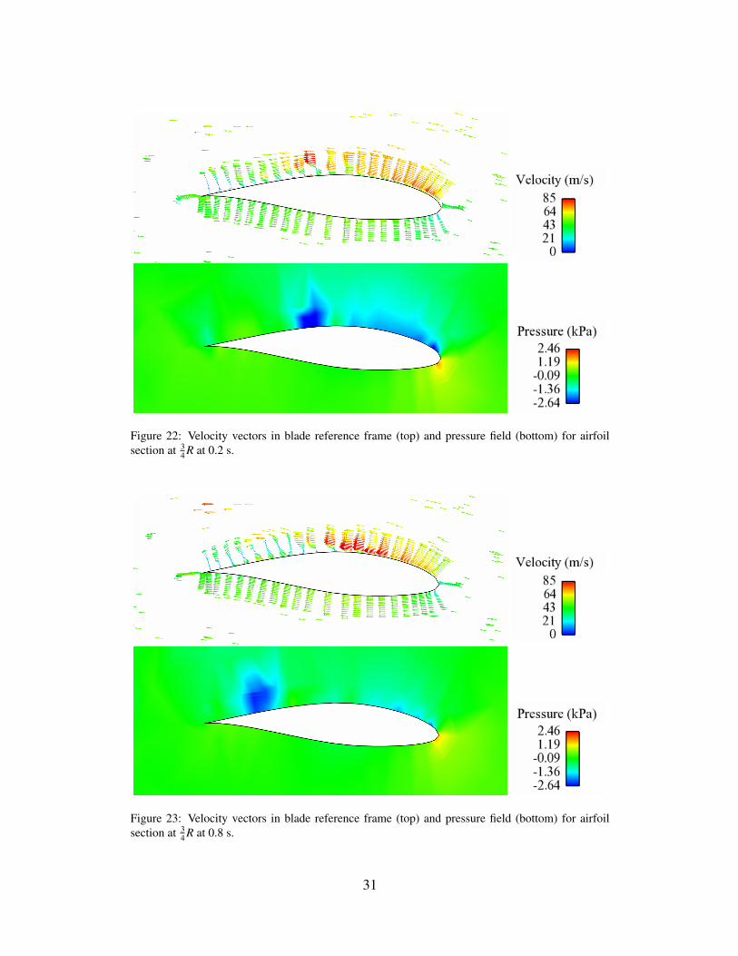
Figure 22: Velocity vectors in blade reference frame (top) and pressure field (bottom) for airfoilsection at 3

4 R at 0.2 s.

Figure 23: Velocity vectors in blade reference frame (top) and pressure field (bottom) for airfoilsection at 3

4 R at 0.8 s.

31

Figure 24: Velocity vectors in blade reference frame (top) and pressure field (bottom) for airfoilsection at center of Patch 17 at 0.2 s.

Figure 25: Velocity vectors in blade reference frame (top) and pressure field (bottom) for airfoilsection at center of Patch 17 at 0.8 s.

32

5.4. Coupled air flow and rigid rotor simulation

Time (s)0 0.2 0.4 0.6 0.8 10

1

2

3

4

Angular velocity (rad/s)

Angular acceleration (rad/s2)

Figure 26: Time history of the rotor angular velocity and acceleration.

In this section, we perform a coupled aerodynamic analysis of the same NREL5MW offshore baseline wind turbine using a NURBS discretization. The windspeed at the inflow is now set to 12 m/s. Reference [61] reports that at this windspeed the rotor blades are pitched to prevent over-rotation. Our interest was to studya scenario in which no blade pitching controls are applied and the rotor is free to spinunder the influence of incoming wind. This situation may occur due to the failureof the rotor control system, in which case, under the prescribed wind condition, therotor will spin at speeds much faster than the limits set by the design strength of therotor structure.

The simulation is started with the rotor spinning at a prescribed angular veloc-ity of 0.8 rad/s. Then the rotor is released to spin freely under the action of windforces. We neglect the frictional losses and interaction with the generator, that is,we set f (θ, t) = 0 in Eq. (22). Figure 26 shows the time history of the rotor angularspeed and acceleration. Within 1 s the rotor attains an angular velocity of 3 rad/s.The computation was stopped at this point, however, the rotor continues to accel-erate. Due to the size and the dimension of the blade, such rotor speeds lead tounsustainable structural loads and, ultimately, wind turbine failure.

Figure 27 shows a snapshot of the rotor spinning at nearly 3 rad/s and the iso-surfaces of the air speed. The trailing edge of the blade and especially the tip createsignificant amount of turbulence. Snapshots of air pressure on the front and back ofthe blade are shown in Figure 28. Note that, compared to the previous case of 9 m/swind and 1.08 rad/s rotation, the pressure magnitude is significantly higher. Fur-thermore, the pressure field at the trailing edge and the blade tip exhibits fluctuating

33

Figure 27: Isosurfaces of air speed at t = 0.8 s.

behavior, which leads to high-frequency loading and aerodynamic noise generationin these areas.

34

(a) Front (b) Back

Figure 28: Air pressure distribution on the blade surface.

35

6. Conclusions

This two-part paper presents a comprehensive computational framework for ad-vanced simulation of wind turbines at full scale and its application to the NREL5MW offshore baseline wind turbine. Part 1 of the paper focused on the wind tur-bine geometry modeling, mesh generation, and numerical simulation in which therotor is assumed to be rigid. Isogeometric analysis was adopted as the primarygeometry modeling and simulation framework. A template-based approach was de-veloped in which the analysis-suitable geometry for both fluid and structural windturbine rotor domains is constructed. The fluid and structural meshes are compatibleat the interface and may be employed for the coupled FSI analysis, which is pre-sented in Part 2 of this paper. The residual-based variational multiscale formulationwas employed for the fluid simulation and turbulence modeling. The quasi-staticassumption on the fine scales was generalized to moving domain problems in theALE framework leading to a formulation that globally conserves linear momentum.

Partial validation of the turbulence modeling technique was performed on a tur-bulent Taylor–Couette flow, which has features in common with wind turbine flows,such as rotation, curved solid walls, and boundary layers. Comparison of linear fi-nite elements and quadratic NURBS revealed the superior per-degree-of-freedomaccuracy of the NURBS-based discretization. Accurate mean flow results are ob-tained even for very coarse meshes with no boundary layer resolution. Weakly-imposed boundary conditions were employed in this simulation and were partlyresponsible for the good quality of the computational results.

Further validation of the proposed method was performed by computing theNREL 5MW offshore baseline wind turbine rotor at full scale. Both NURBS andstandard finite elements were employed for this simulation. The NURBS-basedrepresentation of the wind turbine geometry was used to create a tetrahedral meshfor the FEM simulation, which is an added benefit of the isogeometric framework.The results for aerodynamic torque, a key quantity in evaluating the wind turbineperformance, were in close agreement with those reported in [61] for the NURBSsimulation. This suggests that 3D, complex-geometry, time-dependent computa-tional modeling of wind turbine rotors, which is fully predictive and does not relyon empiricism, is capable of accurately approximating the aerodynamic quantitiesof interest while keeping the number of degrees of freedom at a manageable level.The tetrahdral discretization, which used a significantly smaller number of degreesof freedom, produced a somewhat lower value of the torque than anticipated due tothe premature flow separation that starts near the blade tip and spreads. The resultsof the tetrahedral simulation are expected to improve with further mesh refinement.

The computational framework was extended to coupling of the flow with a ro-tating rigid body, and successfully applied to the simulation of the wind turbinerotor over-spinning under high wind speed inlet conditions. Such computation, per-formed using the NURBS-based discretization, would not be possible with the cur-rently existing methods and tools for wind wind turbine simulation.

36

In the future work we plan to employ weak imposition of Dirichlet boundaryconditions for wind turbine simulations, thus reducing the computational cost as-sociated with boundary layer refinement and increasing accuracy. We also planto incorporate the effect of the wind turbine tower in the simulations, which mayhave considerable influence on the results. It should be noted that the presence ofthe tower will preclude the use of rotationally-periodic boundary conditions, whichwill increase computational cost. Given the advanced nature of the simulations, theproposed framework may be developed further and used for rotor control and bladegeometry optimization. Mesh refinement to increase the accuracy of the tetrahedralsimulations is also planned.

Acknowledgement

We wish to thank the Texas Advanced Computing Center (TACC) at the Uni-versity of Texas at Austin for providing HPC resources that have contributed to theresearch results reported within this paper. M.-C. Hsu was partially supported by theLos Alamos - UC San Diego Educational Collaboration Fellowship. This supportis gratefully acknowledged. This research was supported in part by the Rice Com-putational Research Cluster funded by NSF under Grant CNS-0821727. We thankCreighton Moorman for his help in the very early stages of the FEM simulations.

References

[1] C.A. Walford. Wind turbine reliability: Understanding and minimizing windturbine O & M costs. Technical Report SAND2006-1100, Sandia NationalLaboratories, 2006.

[2] E. Echavarria, B. Hahn, and G.J.W. van Bussel. Reliability of wind turbinetechnology through time. Journal of Solar Energy Engineering, 130, 2008.

[3] M. Bischoff, W. A. Wall, K. -U. Bletzinger, and E. Ramm. Models and finiteelements for thin-walled structures. In E. Stein, R. de Borst, and T. J. R.Hughes, editors, Encyclopedia of Computational Mechanics, Vol. 2, Solids,Structures and Coupled Problems, chapter 3. Wiley, 2004.

[4] T.J.R. Hughes, J.A. Cottrell, and Y. Bazilevs. Isogeometric analysis: CAD,finite elements, NURBS, exact geometry, and mesh refinement. ComputerMethods in Applied Mechanics and Engineering, 194:4135–4195, 2005.

[5] J.A. Cottrell, A. Reali, Y. Bazilevs, and T.J.R. Hughes. Isogeometric anal-ysis of structural vibrations. Computer Methods in Applied Mechanics andEngineering, 195:5257–5297, 2006.

[6] Y. Bazilevs, L. Beirao da Veiga, J.A. Cottrell, T.J.R. Hughes, and G. San-galli. Isogeometric analysis: Approximation, stability and error estimates for

37

h-refined meshes. Mathematical Models and Methods in Applied Sciences,16:1031–1090, 2006.

[7] J.A. Cottrell, T.J.R. Hughes, and A. Reali. Studies of refinement and conti-nuity in isogeometric structural analysis. Computer Methods in Applied Me-chanics and Engineering, 196:4160–4183, 2007.

[8] W. A. Wall, M. A. Frenzel, and C. Cyron. Isogeometric structural shapeoptimization. Computer Methods in Applied Mechanics and Engineering,197:2976–2988, 2008.

[9] J.A. Cottrell, T.J.R. Hughes, and Y. Bazilevs. Isogeometric Analysis: TowardIntegration of CAD and FEA. Wiley, Chichester, 2009.

[10] J.A. Evans, Y. Bazilevs, I. Babuska, and T.J.R. Hughes. N-widths, sup-infs, and optimality ratios for the k-version of the isogeometric finite ele-ment method. Computer Methods in Applied Mechanics and Engineering,198:1726–1741, 2009.

[11] M.R. Dorfel, B. Juttler, and B. Simeon. Adaptive isogeometric analysis bylocal h-refinement with T-splines. Computer Methods in Applied Mechanicsand Engineering, 199:264–275, 2010.

[12] Y. Bazilevs, V.M. Calo, J.A. Cottrell, J.A. Evans, T.J.R. Hughes, S. Lipton,M.A. Scott, and T.W. Sederberg. Isogeometric analysis using T-splines. Com-puter Methods in Applied Mechanics and Engineering, 199:264–275, 2010.

[13] F. Auricchio, L. Beirao da Veiga, C. Lovadina, and A. Reali. The importanceof the exact satisfaction of the incompressibility constraint in nonlinear elastic-ity: Mixed FEMs versus NURBS-based approximations. Computer Methodsin Applied Mechanics and Engineering, 199:314–323, 2010.

[14] W. Wang and Y. Zhang. Wavelets-based NURBS simplification and fair-ing. Computer Methods in Applied Mechanics and Engineering, 199:290–300,2010.

[15] E. Cohen, T. Martin, R.M. Kirby, T. Lyche, and R.F. Riesenfeld. Analysis-aware modeling: Understanding quality considerations in modeling for isoge-ometric analysis. Computer Methods in Applied Mechanics and Engineering,199:334–356, 2010.

[16] V. Srinivasan, S. Radhakrishnan, and G. Subbarayan. Coordinated synthesisof hierarchical engineering systems. Computer Methods in Applied Mechanicsand Engineering, 199:392–404, 2010.

38

[17] Y. Bazilevs, V.M. Calo, J.A. Cottrel, T.J.R. Hughes, A. Reali, and G. Scov-azzi. Variational multiscale residual-based turbulence modeling for large eddysimulation of incompressible flows. Computer Methods in Applied Mechanicsand Engineering, 197:173–201, 2007.

[18] Y. Bazilevs, C. Michler, V.M. Calo, and T.J.R. Hughes. Weak Dirichlet bound-ary conditions for wall-bounded turbulent flows. Computer Methods in Ap-plied Mechanics and Engineering, 196:4853–4862, 2007.

[19] Y. Bazilevs, C. Michler, V.M. Calo, and T.J.R. Hughes. Isogeometric vari-ational multiscale modeling of wall-bounded turbulent flows with weakly-enforced boundary conditions on unstretched meshes. Computer Methods inApplied Mechanics and Engineering, 2010. doi:10.1016/j.cma.2008.11.020.

[20] I. Akkerman, Y. Bazilevs, V.M. Calo, T.J.R. Hughes, and S. Hulshoff. The roleof continuity in residual-based variational multiscale modeling of turbulence.Computational Mechanics, 41:371–378, 2008.

[21] M.-C. Hsu, Y. Bazilevs, V.M. Calo, T.E. Tezduyar, and T.J.R. Hughes. Im-proving stability of stabilized and multiscale formulations in flow simulationsat small time steps. Computer Methods in Applied Mechanics and Engineer-ing, 199:828–840, 2010.

[22] Y. Bazilevs and I. Akkerman. Large eddy simulation of turbulent Taylor–Couette flow using isogeometric analysis and the residual–based variationalmultiscale method. Journal of Computational Physics, 229:3402–3414, 2010.

[23] T. Elguedj, Y. Bazilevs, V.M. Calo, and T.J.R. Hughes. Bbar and Fbar pro-jection methods for nearly incompressible linear and non-linear elasticity andplasticity using higher-order NURBS elements. Computer Methods in AppliedMechanics and Engineering, 197:2732–2762, 2008.

[24] S. Lipton, J.A. Evans, Y. Bazilevs, T. Elguedj, and T.J.R. Hughes. Robustnessof isogeometric structural discretizations under severe mesh distortion. Com-puter Methods in Applied Mechanics and Engineering, 199:357–373, 2010.

[25] D.J. Benson, Y. Bazilevs, E. De Luycker, M.-C. Hsu, M. Scott, T.J.R. Hughes,and T. Belytschko. A generalized finite element formulation for arbitrary basisfunctions: from isogeometric analysis to XFEM. International Journal forNumerical Methods in Engineering, 2010. DOI: 10.1002/nme.2864.

[26] D.J. Benson, Y. Bazilevs, M.C. Hsu, and T.J.R. Hughes. Isogeometric shellanalysis: The Reissner–Mindlin shell. Computer Methods in Applied Mechan-ics and Engineering, 199:276–289, 2010.

39

[27] J. Kiendl, K.-U. Bletzinger, J. Linhard, and R. Wuchner. Isogeometric shellanalysis with Kirchhoff–Love elements. Computer Methods in Applied Me-chanics and Engineering, 198:3902–3914, 2009.

[28] J. Kiendl, Y. Bazilevs, M.-C. Hsu, R. Wuchner, and K.-U. Bletzinger. Thebending strip method for isogeometric analysis of kirchhoff-love shell struc-tures comprised of multiple patches. Computer Methods in Applied Mechanicsand Engineering, 2010. doi:10.1016/j.cma.2010.03.029.

[29] Y. Zhang, Y. Bazilevs, S. Goswami, C. Bajaj, and T.J.R. Hughes. Patient-specific vascular NURBS modeling for isogeometric analysis of blood flow.Computer Methods in Applied Mechanics and Engineering, 196:2943–2959,2007.

[30] Y. Bazilevs, V.M. Calo, Y. Zhang, and T.J.R. Hughes. Isogeometric fluid-structure interaction analysis with applications to arterial blood flow. Compu-tational Mechanics, 38:310–322, 2006.

[31] Y. Bazilevs, V.M. Calo, T.J.R. Hughes, and Y. Zhang. Isogeometric fluid-structure interaction: theory, algorithms, and computations. ComputatonalMechanics, 43:3–37, 2008.

[32] J.G. Isaksen, Y. Bazilevs, T. Kvamsdal, Y. Zhang, J.H. Kaspersen, K. Wa-terloo, B. Romner, and T. Ingebrigtsen. Determination of wall tension incerebral artery aneurysms by numerical simulation. Stroke, 2008. DOI:10.1161/STROKEAHA.107.503698.

[33] Y. Bazilevs and T.J.R. Hughes. NURBS-based isogeometric analysis for thecomputation of flows about rotating components. Computatonal Mechanics,43:143–150, 2008.

[34] T. E. Tezduyar. Stabilized finite element formulations for incompressible flowcomputations. Advances in Applied Mechanics, 28:1–44, 1992.

[35] T. E. Tezduyar, M. Behr, and J. Liou. A new strategy for finite element com-putations involving moving boundaries and interfaces – the deforming-spatial-domain/space–time procedure: I. The concept and the preliminary numericaltests. Computer Methods in Applied Mechanics and Engineering, 94(3):339–351, 1992.

[36] T. E. Tezduyar, M. Behr, S. Mittal, and J. Liou. A new strategy for fi-nite element computations involving moving boundaries and interfaces – thedeforming-spatial-domain/space–time procedure: II. Computation of free-surface flows, two-liquid flows, and flows with drifting cylinders. ComputerMethods in Applied Mechanics and Engineering, 94(3):353–371, 1992.

40

[37] T.E. Tezduyar. Computation of moving boundaries and interfaces and stabi-lization parameters. International Journal for Numerical Methods in Fluids,43:555–575, 2003.

[38] T. E. Tezduyar and S. Sathe. Modeling of fluid–structure interactions withthe space–time finite elements: Solution techniques. International Journal forNumerical Methods in Fluids, 54:855–900, 2007.

[39] S. Mittal and T. E. Tezduyar. A finite element study of incompressible flowspast oscillating cylinders and aerofoils. International Journal for NumericalMethods in Fluids, 15:1073–1118, 1992.

[40] S. Mittal and T. E. Tezduyar. Parallel finite element simulation of 3D in-compressible flows – Fluid-structure interactions. International Journal forNumerical Methods in Fluids, 21:933–953, 1995.

[41] V. Kalro and T. E. Tezduyar. A parallel 3D computational method for fluid–structure interactions in parachute systems. Computer Methods in AppliedMechanics and Engineering, 190:321–332, 2000.

[42] K. Stein, R. Benney, V. Kalro, T. E. Tezduyar, J. Leonard, and M. Accorsi.Parachute fluid–structure interactions: 3-D Computation. Computer Methodsin Applied Mechanics and Engineering, 190:373–386, 2000.

[43] T. Tezduyar and Y. Osawa. Fluid–structure interactions of a parachute crossingthe far wake of an aircraft. Computer Methods in Applied Mechanics andEngineering, 191:717–726, 2001.

[44] T.E. Tezduyar, S. Sathe, R. Keedy, and K. Stein. Space–time finite elementtechniques for computation of fluid–structure interactions. Computer Methodsin Applied Mechanics and Engineering, 195:2002–2027, 2006.

[45] T. E. Tezduyar, S. Sathe, and K. Stein. Solution techniques for the fully-discretized equations in computation of fluid–structure interactions with thespace–time formulations. Computer Methods in Applied Mechanics and En-gineering, 195:5743–5753, 2006.

[46] T. E. Tezduyar, S. Sathe, T. Cragin, B. Nanna, B. S. Conklin, J. Pausewang,and M. Schwaab. Modeling of fluid–structure interactions with the space–timefinite elements: Arterial fluid mechanics. International Journal for NumericalMethods in Fluids, 54:901–922, 2007.

[47] T. E. Tezduyar, S. Sathe, M. Schwaab, and B. S. Conklin. Arterial fluid me-chanics modeling with the stabilized space–time fluid–structure interactiontechnique. International Journal for Numerical Methods in Fluids, 57:601–629, 2008.

41

[48] T. E. Tezduyar, S. Sathe, J. Pausewang, M. Schwaab, J. Christopher, andJ. Crabtree. Interface projection techniques for fluid–structure interactionmodeling with moving-mesh methods. Computational Mechanics, 43:39–49,2008.

[49] T. E. Tezduyar, M. Schwaab, and S. Sathe. Sequentially-Coupled ArterialFluid–Structure Interaction (SCAFSI) technique. Computer Methods in Ap-plied Mechanics and Engineering, 198:3524–3533, 2009.

[50] T. E. Tezduyar, K. Takizawa, C. Moorman, S. Wright, and J. Christopher.Multiscale sequentially-coupled arterial FSI technique. Computational Me-chanics, 46:17–29, 2010.

[51] T. E. Tezduyar, K. Takizawa, C. Moorman, S. Wright, and J. Christopher.Space–time finite element computation of complex fluid–structure interac-tions. International Journal for Numerical Methods in Fluids, published on-line, DOI: 10.1002/d.2221, 2009.

[52] K. Takizawa, J. Christopher, T. E. Tezduyar, and S. Sathe. Space–time finite el-ement computation of arterial fluid–structure interactions with patient-specificdata. International Journal for Numerical Methods in Biomedical Engineer-ing, 26:101–116, 2010.

[53] K. Takizawa, C. Moorman, S. Wright, J. Christopher, and T. E. Tezduyar. Wallshear stress calculations in space–time finite element computation of arterialfluid–structure interactions. Computational Mechanics, 46:31–41, 2010.

[54] K. Takizawa, C. Moorman, S. Wright, T. Spielman, and T. E. Tezduyar. Fluid–structure interaction modeling and performance analysis of the Orion space-craft parachutes. International Journal for Numerical Methods in Fluids, pub-lished online, DOI: 10.1002/d.2348, May 2010.

[55] K. Takizawa, C. Moorman, S. Wright, J. Purdue, T. McPhail, P. R. Chen,J. Warren, and T. E. Tezduyar. Patient-specific arterial fluid–structure inter-action modeling of cerebral aneurysms. International Journal for NumericalMethods in Fluids, published online, DOI: 10.1002/d.2360, May 2010.

[56] K. Takizawa, S. Wright, C. Moorman, and T. E. Tezduyar. Fluid–structure in-teraction modeling of parachute clusters. International Journal for NumericalMethods in Fluids, published online, DOI: 10.1002/d.2359, May 2010.

[57] T. E. Tezduyar, S. Sathe, J. Pausewang, M. Schwaab, J. Christopher, andJ. Crabtree. Fluid–structure interaction modeling of ringsail parachutes. Com-putational Mechanics, 43:133–142, 2008.

42

[58] T. Tezduyar, S. Aliabadi, M. Behr, A. Johnson, V. Kalro, and M. Litke.Flow simulation and high performance computing. Computational Mechanics,18:397–412, 1996.

[59] M. Behr and T. Tezduyar. The Shear-Slip Mesh Update Method. ComputerMethods in Applied Mechanics and Engineering, 174:261–274, 1999.

[60] M. Behr and T. Tezduyar. Shear-slip mesh update in 3D computation of com-plex flow problems with rotating mechanical components. Computer Methodsin Applied Mechanics and Engineering, 190:3189–3200, 2001.

[61] J. Jonkman, S. Butterfield, W. Musial, and G. Scott. Definition of a 5-MWreference wind turbine for offshore system development. Technical ReportNREL/TP-500-38060, National Renewable Energy Laboratory, Golden, CO,2009.

[62] E. Hau. Wind Turbines: Fundamentals, Technologies, Application, Eco-nomics. 2nd Edition. Springer, Berlin, 2006.

[63] H.J.T. Kooijman, C. Lindenburg, D. Winkelaar, and E.L. van der Hooft.DOWEC 6 MW pre-design: Aero-elastic modelling of the DOWEC 6 MWpre-design in PHATAS. Technical Report DOWEC-F1W2-HJK-01-046/9,2003.

[64] J.M. Jonkman and M.L. Buhl Jr. FAST user’s guide. Technical ReportNREL/EL-500-38230, National Renewable Energy Laboratory, Golden, CO,2005.

[65] T. J. R. Hughes. Multiscale phenomena: Green’s functions, the Dirichlet-to-Neumann formulation, subgrid scale models, bubbles and the origins of sta-bilized methods. Computer Methods in Applied Mechanics and Engineering,127:387–401, 1995.

[66] T. J. R. Hughes, G. Feijoo., L. Mazzei, and J. B. Quincy. The variationalmultiscale method – A paradigm for computational mechanics. ComputerMethods in Applied Mechanics and Engineering, 166:3–24, 1998.

[67] A.N. Brooks and T.J.R. Hughes. Streamline upwind/Petrov-Galerkin formula-tions for convection dominated flows with particular emphasis on the incom-pressible Navier-Stokes equations. Computer Methods in Applied Mechanicsand Engineering, 32:199–259, 1982.

[68] T.J.R Hughes and T.E. Tezduyar. Finite element methods for first-order hy-perbolic systems with particular emphasis on the compressible Euler equa-tions. Computer Methods in Applied Mechanics and Engineering, 45:217–284, 1984.

43

[69] T. E. Tezduyar and Y. J. Park. Discontinuity capturing finite element for-mulations for nonlinear convection-diffusion-reaction equations. ComputerMethods in Applied Mechanics and Engineering, 59:307–325, 1986.

[70] T. E. Tezduyar, S. Mittal, S. E. Ray, and R. Shih. Incompressible flow compu-tations with stabilized bilinear and linear equal-order-interpolation velocity-pressure elements. Computer Methods in Applied Mechanics and Engineer-ing, 95:221–242, 1992.

[71] L. P. Franca and S. Frey. Stabilized finite element methods: II. The incom-pressible Navier-Stokes equations. Computer Methods in Applied Mechanicsand Engineering, 99:209–233, 1992.

[72] T. E. Tezduyar and Y. Osawa. Finite element stabilization parameters com-puted from element matrices and vectors. Computer Methods in Applied Me-chanics and Engineering, 190:411–430, 2000.

[73] T.J.R. Hughes, G. Scovazzi, and L.P. Franca. Multiscale and stabilized meth-ods. In E. Stein, R. de Borst, and T. J. R. Hughes, editors, Encyclopedia ofComputational Mechanics, Vol. 3, Computational Fluid Dynamics, chapter 2.Wiley, 2004.

[74] L. Catabriga, A. L. G. A. Coutinho, and T. E. Tezduyar. Compressible flowSUPG parameters computed from degree-of-freedom submatrices. Computa-tional Mechanics, 38:334–343, 2006.

[75] T.J.R. Hughes and G. Sangalli. Variational multiscale analysis: the fine-scaleGreen’s function, projection, optimization, localization, and stabilized meth-ods. SIAM Journal of Numerical Analysis, 45:539–557, 2007.

[76] Y. Bazilevs and T.J.R. Hughes. Weak imposition of Dirichlet boundary condi-tions in fluid mechanics. Computers and Fluids, 36:12–26, 2007.

[77] R. Calderer and A. Masud. A multiscale stabilized ALE formulation forincompressible flows with moving boundaries. Computational Mechanics,46:185–197, 2010.

[78] G. Lewis and H. Swinney. Velocity structure functions, scaling and transitionsin high-Reynolds-number Couette–Taylor flow. Phys. Rev. E, 59:5457–5467,1999.

[79] T. Tezduyar, S. Aliabadi, M. Behr, A. Johnson, and S. Mittal. Parallel finiteelement computation of 3D flows. Computer, 26:27–36, 1993.

[80] T.E. Tezduyar, S.K. Aliabadi, M. Behr, and S. Mittal. Massively parallel fi-nite element simulation of compressible and incompressible flows. ComputerMethods in Applied Mechanics and Engineering, 119:157–177, 1994.

44

[81] M. Bilson and K. Bremhorst. Direct numerical simulation of turbulent Taylor-Couette flow. Journal of Fluid Mechanics, 579:227–270, 2007.

[82] D. Pirro and M. Quadrio. Direct numerical simulation of turbulent Taylor-Couette flow. European Journal of Mechanics - B/Fluids, 27:552–566, 2007.

[83] S. Dong. Turbulent flow between counter-rotating concentric cylinders: ADNS study. Journal of Fluid Mechanics, 615:371–399, 2008.

[84] S. B. Pope. Large-eddy simulation using projection onto local basis functions.In J. L. Lumley, editor, Fluid Mechanics and the Environment: DynamicalApproaches. Springer, 2000. To appear.

[85] C.G. Speziale, B.A. Younis, R. Rubinstein, and Y. Zhou. On consistency con-ditions for rotating turbulent flows. Physics of Fluids, 10:2108–2110, 1998.

[86] S. Dong. DNS of turbulent Taylor-Couette flow. Journal of Fluid Mechanics,587:373–393, 2007.

[87] R.M. Kirby and G.E. Karniadakis. Spectral element and hp methods. InE. Stein, R. de Borst, and T. J. R. Hughes, editors, Encyclopedia of Com-putational Mechanics, Vol. 3, Computational Fluid Dynamics. Wiley, 2004.

[88] J. Jeong and F. Hussain. On the identification of a vortex. Journal of FluidMechanics, 285:69–94, 1995.

[89] K. E. Jansen, C. H. Whiting, and G. M. Hulbert. A generalized-α method forintegrating the filtered Navier-Stokes equations with a stabilized finite elementmethod. Computer Methods in Applied Mechanics and Engineering, 190:305–319, 1999.

[90] J. Chung and G. M. Hulbert. A time integration algorithm for structuraldynamics with improved numerical dissipation: The generalized-α method.Journal of Applied Mechanics, 60:371–75, 1993.

[91] K. Takizawa, C. Moorman, S. Wright, and T. E. Tezduyar. Computer modelingand analysis of the Orion spacecraft parachutes. In Hans-Joachim Bungartzand M. Schafer, editors, Fluid–Structure Interaction – Modelling, Simulation,Optimization, Part II, Lecture Notes in Computational Science and Engineer-ing. Springer, 2010.

[92] D. A. Spera. Introduction to modern wind turbines. In D. A. Spera, editor,Wind Turbine Technology: Fundamental Concepts of Wind Turbine Engineer-ing, pages 47–72. ASME Press, 1994.

[93] Texas Advanced Computing Center (TACC). http://www.tacc.utexas.edu.

45

[94] Y. Saad and M. Schultz. GMRES: A generalized minimal residual algorithmfor solving nonsymmetric linear systems. SIAM Journal of Scientific and Sta-tistical Computing, 7:856–869, 1986.

[95] G. Karypis and V. Kumar. A fast and high quality multilevel scheme for parti-tioning irregular graphs. SIAM Journal of Scientific Computing, 20:359–392,1998.

[96] F. Rispoli, A. Corsini, and T. E. Tezduyar. Finite element computation of tur-bulent flows with the discontinuity-capturing directional dissipation (DCDD).Computers & Fluids, 36:121–126, 2007.

[97] J. Smagorinsky. General circulation experiments with the primitive equations.Monthly Weather Review, 91(3):99–165, 1963.

[98] T. E. Tezduyar, S. Ramakrishnan, and S. Sathe. Stabilized formulations forincompressible flows with thermal coupling. International Journal for Nu-merical Methods in Fluids, 57:1189–1209, 2008.

46