3d video transmission over lte
TRANSCRIPT
Lucas García Cillanueva
3D video transmission over LTE
Dissertação de Mestrado
14 de Fevereiro de 2014


FACULDADE DE CIÊNCIAS E TECNOLOGIA DA
UNIVERSIDADE DE COIMBRA
MESTRADO INTEGRADO EM ENGENHARIA
ELECTROTÉCNICA E DE COMPUTADORES
3D Video Transmission over LTE
Lucas García Cillanueva
Júri
Presidente: Professor Vítor Manuel Mendes da Silva
Vogal: Professor António Paulo Mendes Breda Dias Coimbra
Orientador: Professor Luís Alberto da Silva Cruz
Coimbra, 14 de Fevereiro de 2014


Abstract
This thesis presents a research work on quality of experience in 3D video transmission
over LTE networks. The objective is to study the state-of-art of LTE and 3D video,
described in the scientific literature, and to quantify the user quality of experience
(QoE) during a simulated LTE transmission.
The work will start by a study of the University of Wien “LTE-A System Simulator”
and its capabilities. In addition, different scenarios with various users equipment (UEs)
and base stations (eNodeBs) densities will be configured and simulated in order to
obtain the frame-by-frame Block Error Rate (BLER) values experienced by different
UEs.
Once obtained, the Block Error Rate frames will be converted to packet level error
traces, which will be used to introduce erasures and corruptions into the packetized 3D
video bitstream.
The corrupted encoded video stream will be decoded using an error-concealment
capable video decoder and the decoded/recovered video quality (QoE) will be estimated
based on the Structural Similarity Index of the recovered video.
Finally, the QoE results for the different system configurations will allow classifying
the severity of the QoE degradations due to transmission losses, through inferring the
relationship between those system parameters and the achievable QoE.
Keywords: 3D Video, Quality of Experience, Long Term Evolution, Evolved Node B,
User Equipment, Block Error Rate, Structural Similarity Index.


Resumo
Esta dissertação apresenta um trabalho de investigação sobre a qualidade de experiência
numa transmissão de vídeo 3D sobre redes LTE. O objectivo é estudar o estado-da-arte
no que respeita a rede LTE e vídeo 3D, descrito na literatura científica, e obter a
qualidade de experiência de usuário (QoE) durante uma simulação de transmissão LTE.
O trabalho começará por um estudo do University of Wien “LTE-A System Simulator”
e as suas capacidades. Para este efeito, vão ser configurados diferentes cenários com
distintas densidades de utilizadores (UEs) e estações base (eNodeBs), com o fim de
obter a taxa de erros do bloco (BLER) experimentada por diferentes utilizadores.
Depois de obter esta taxa, as tramas da taxa de erros do bloco (BLER) serão convertidas
em tramas de nível de erro de pacotes, que vão ser usadas para adicionar corrupções de
bit em ficheiros de vídeo 3D.
O fluxo de vídeo codificado e corrompido será descodificado usando um descodificador
de vídeo e a qualidade do vídeo recuperado vai ser calculada com base no Índice de
Similitude Estrutural.
Finalmente, os resultados de QoE para as diferentes configurações do sistema
permitirão classificar o nível das degradações de QoE devido a perdas de transmissão,
por meio de inferir a relação entre os parâmetros do sistema e a QoE obtida.
Palavras-chave: Vídeo 3D, Qualidade de experiência do Usuário, Evolução de Longo
Prazo, utilizador LTE, Taxa de Erros de Bloco, Índice de Similitude Estrutural.


i
Contents
Abstract .................................................................................................................................... 2
Resumo ..................................................................................................................................... 4
Contents .................................................................................................................................... i
List of Figures ......................................................................................................................... v
List of Tables ......................................................................................................................... vii
List of Acronyms and Abbreviations ............................................................................. ix
1. Introduction ....................................................................................................................... 1
1.1. Context ....................................................................................................................................... 1
1.2. Outline of the dissertation .................................................................................................. 2
2. LTE System Overview ...................................................................................................... 3
2.1 Key features of LTE ................................................................................................................. 4
2.2. Network architecture ........................................................................................................... 6
2.3. Protocol architecture ........................................................................................................... 7
2.3.1. Radio Link Control ........................................................................................................................... 9
2.3.2. Medium Access Control .............................................................................................................. 10
3. LTE Physical Layer ........................................................................................................ 14
3.1. LTE frame structure ............................................................................................................ 15
3.1.1. OFDMA ............................................................................................................................................... 15

ii
3.1.2. SC-‐FDMA ........................................................................................................................................... 18
3.2. Multi-‐Antenna techniques ................................................................................................ 19
3.2.1. Multiple transmit antennas ...................................................................................................... 19
3.2.2. Spatial multiplexing ..................................................................................................................... 20
4. 3D Video transmissions ............................................................................................... 23
4.1. State-‐of-‐art ............................................................................................................................. 23
4.2. 3D video system ................................................................................................................... 24
4.2.1. 3D content creation ...................................................................................................................... 24
4.2.2. 3D representation ......................................................................................................................... 24
4.2.3. Delivery ............................................................................................................................................. 28
4.2.4. Visualization .................................................................................................................................... 28
4.3. Objective quality metrics of 3D video ........................................................................... 30
4.3.1. Media-‐layer FR image quality models .................................................................................. 31
5. Methods, tools and simulated scenario ................................................................. 33
5.1. The University of Vienna System Level LTE Simulator ........................................... 33
5.1.1. Using the simulator ...................................................................................................................... 35
5.2. Evaluated scenarios ............................................................................................................ 39
6. Experiments and results ............................................................................................. 41
6.1. Simulator output results ................................................................................................... 42
6.1.1. Balloons ............................................................................................................................................. 42

iii
6.1.2. Kendo ................................................................................................................................................. 42
6.1.3. Lovebird ............................................................................................................................................ 43
6.1.4. Newspaper ....................................................................................................................................... 43
6.1.5. Overview .......................................................................................................................................... 44
6.2. QoE results ............................................................................................................................. 46
6.2.1. Balloons ............................................................................................................................................. 46
6.2.2. Kendo ................................................................................................................................................. 46
6.2.3. Lovebird ............................................................................................................................................ 47
6.2.4. Newspaper ....................................................................................................................................... 47
6.2.5. Overview ........................................................................................................................................... 48
6.3. Analysis of the results ........................................................................................................ 49
7. Conclusion ........................................................................................................................ 51
References ............................................................................................................................ 53

iv

v
List of Figures
Figure 1 - Relative subscriptions in mobile technologies ................................................ 5
Figure 2 - LTE network architecture ................................................................................ 7
Figure 3 - LTE Protocol stack and main functions .......................................................... 7
Figure 4 - Overview of the LTE protocol architecture for downlink ............................... 8
Figure 5 - Radio Link Control PDU ................................................................................ 10
Figure 6 - Flow of downlink data through all the protocol layers .................................. 13
Figure 7 - LTE Generic Frame Structure ....................................................................... 16
Figure 8 - Resource blocks for uplink and downlink ...................................................... 17
Figure 9 - LTE resource block vs. resource element ..................................................... 17
Figure 10 - Diversity channel with an M-element transmit antenna array ..................... 20
Figure 11 - Classical beam-forming with high mutual antennas correlation ................. 20
Figure 12 - Downlink transmission in MU-MIMO configuration ................................. 22
Figure 13 - Structure of an end-to-end 3D video system ................................................ 24
Figure 14 - Image-based representation .......................................................................... 25
Figure 15 - DIBR procedure ........................................................................................... 27
Figure 16 - MVD System ............................................................................................... 27
Figure 17 - Simulated scenario ........................................................................................ 33
Figure 18 - Schematic block diagram of the simulator .................................................. 34

vi
Figure 19 - CQI vs. BLER curves and CQI from the 10% BLER points ....................... 35
Figure 20 - UEs network configured (30 UEs per eNodeB) ........................................... 36
Figure 21 - Base station positions ................................................................................... 37
Figure 22 - UE positions for 5km/h ................................................................................ 37
Figure 23 - UE position for 36km/h ................................................................................ 38
Figure 24 - UE positions for 72km/h .............................................................................. 38
Figure 25 - Diagram of the evaluated scenario ............................................................... 39
Figure 27 - Block Diagram of the BLER conversion ...................................................... 40
Figure 28 - PLR results for Balloons .............................................................................. 42
Figure 29 - PLR results for Kendo .................................................................................. 42
Figure 30 - PLR results for Lovebird .............................................................................. 43
Figure 31 - PLR results for Newspaper ........................................................................... 43
Figure 32 - QoE results for Balloons .............................................................................. 46
Figure 33 - QoE results for Kendo .................................................................................. 46
Figure 34 - QoE results for Lovebird .............................................................................. 47
Figure 35 - QoE results for Newspaper ........................................................................... 47

vii
List of Tables
Table 1 - Types of Mobiles Stations ................................................................................ 4
Table 2 - PLCC performance comparison of VQA algorithms ...................................... 31
Table 3 - Configuration parameters of the System Simulator ......................................... 36
Table 4 - Encoder setting parameters of the videos used ................................................ 41
Table 5 - PLR results from Balloons ............................................................................... 44
Table 6 - PLR results from Kendo .................................................................................. 44
Table 7 - PLR results from Lovebird .............................................................................. 44
Table 8 - PLR results from Newspaper ........................................................................... 45
Table 9 - SSIM results from Balloons ............................................................................. 48
Table 10 - SSIM results from Kendo .............................................................................. 48
Table 11 - SSIM results from Lovebird .......................................................................... 48
Table 12 - SSIM results from Newspaper ....................................................................... 49

viii

ix
List of Acronyms and Abbreviations
2D Two-dimensional
3D Three-dimensional
3DTV Three-dimensional Television
3GPP 3rd Generation Partnership Project
ARQ Automatic Repeat Request
AVC Advance Video Coding
BS Base Station
BCH Broadcast Channel
BLER Block Error Rate
CQI Channel Quality Identifier
CRC Cyclic Redundancy Check
DCCH Dedicated Control Channel
DIBR Depth-Image-Based Rendering
DL-SCH Downlink Shared Channel
DTCH Dedicated Traffic Channel
EnodeB/eNB Evolved Node B
EPC Evolved Packet Core
EPS Evolved Packet System
FVV Free Viewpoint Video
H.264/AVC ISO/ITU Video Coding Standard
HARQ Hybrid Automatic Repeat Request
HSPA High-Speed Packet Access
IP Internet Protocol
x
LTE Long Term Evolution
MAC Medium Access Control
MBMS Multimedia Broadcast and Multicast Services
MCCH Multicast Control Channel
MCH Multicast Channel
MCS Modulation and Coding Scheme
MIMO Multiple-Input Multiple-Output
MME Mobility Management Entity
MPEG Moving Picture Experts Group
MS Mobile Station
MTCH Multicast Traffic Channel
MVD Multi-view Video plus Depth
OFDM Orthogonal Frequency Division Multiplexing
PAPR Peak-to-Average Power Ratio
PCCH Paging control Channel
PCH Paging Channel
PDCP Packet Data Convergence Protocol
PDN Packet Data Network
PDU Protocol Data Unit
PHY LTE Physical Layer
PLCC Pearson Linear Correlation Coefficient
PLR Packet Loss Ratio
PSNR Peak Signal-to-Noise Ratio
QoE Quality of Experience

xi
RAN Radio Access Network
RB Resource Block
RLC Radio Link Control
ROHC Robust Header Compression
RX Receiver
SAE System Architecture Evolution
SC-FDMA Single-Carrier Frequency Division Multiple Access
SDU Service Data Unit
SGW Serving Gateway
SM Spatial Multiplexing
SSIM Structural Similarity Index Model
SU-MIMO Single User- MIMO
SVC Scalable Video Coding
TTI Transmission Time Interval
UDP User Data Protocol
UE User Equipment
UL Uplink
UL-SCH Uplink Shared Channel
UMTS Universal Mobile Telecommunications System
UTRAN Universal Terrestrial Radio Access Network
V+D Video plus Depth
VQA Video Quality Assessment
WCDMA Wideband Code Division Multiple Access

xii
1
1. Introduction
1.1. Context
Latest developed technologies based in 3D video and image transmission are translated
into an increasing consumer demand for 3D content [6]. Recent studies have anticipated
that the adaptive streaming portion of Internet video will grow at an average of 77% per
year, reaching up to 51% of the network video traffic consumed by 2015. With the main
purpose of delivering the best user experience, adaptive streaming has to optimize the
video configurations during transmission.
3D video provides more realism of the scene, and it involves much more information
needed to transmit the video than the two-dimensional (2D) representation. Thus,
current and future networks should be able to dedicate a large amount of bandwidth to
3D video streaming services.
Immersive and interactive multimedia applications over wireless will be enabled by the
recent LTE standard, thanks to the low latencies and high data rates supported. LTE
emerges as a 3GPP (Third Generation Partnership Project) standard, and enables high
transmission data rates by supporting radio access with up to 100Mbit/s in full mobility
wide area deployments and 1Gbps in low mobility local area deployments [24]. In terms
of the high spectral efficiency, it is located between 5 and 10 b/s/Hz for a single user
and for 2 to 3 b/s/Hz for the multiuser case. This enables reliable wireless transmission
of huge content over the LTE networks.
The latest broadband cellular technology, LTE, allows supporting different services
with high data rates and different Quality of Service requirements. Therefore, it can be
considered a very promising architecture for 3D video transmission.

2
1.2. Outline of the dissertation
Firstly, an overview of LTE technology is presented, with emphasis on the main goals
and key features of LTE. Moreover, the network and protocol architectures will be
introduced.
Section 3 talks about the LTE Physical Layer, the main LTE layer studied in this work.
In section 4, the state-of-art of the 3D technology is explained. For this purpose, the
structure of an end-to-end 3D video system and the different types of the 3D video
representations are mentioned. Additionally, the main quality metrics of 3D video are
enumerated.
Section 5 provides information about the tools used in this scope, with emphasis on the
“University of Wien LTE-A System Simulator”, the main tool employed in this
investigation.
In section 6, the experimental results are described. This section is divided into two
parts: the simulator output results (Packet Loss Ratio results) and the QoE results
(Structural Similarity Index results).
This thesis concludes with section 7, by summarizing the results obtained and drawing
some conclusions.

3
2. LTE System Overview
Long Term Evolution (LTE) has been designed to support only packet-switched
services, contrary to the prior cellular systems, based on circuit-switched models. The
main LTE purpose is to provide IP connectivity between UE (User Equipment) and the
PDN (Packet Data Network) without occurring interruptions of user applications during
connection.
In LTE there is a big change compared to previous mobile technologies, UMTS
(Universal Mobile Telecommunications System) and HSPA (High Speed Packet
Access) due to the introduction of a novel physical layer and the core network reform.
The main reasons for these Radio Access Network (RAN) system design developments
are the requirement to provide higher spectral efficiency, lower delay and more multi-
user flexibility and secure service than the existing deployed networks.
Thus, while LTE includes the evolution of the Universal Mobile Telecommunications
System (UMTS) Radio Access Network by designing the Evolved UTRAN (E-
UTRAN), there is also a development of other aspects, like the System Architecture
Evolution (SAE), which covers the Evolved Packet Core (EPC) network. The Evolved
Packet System (EPS) is included by the LTE and SAE.

4
2.1 Key features of LTE
LTE aims to achieve a peak data rate of 100 Mbit/s to 326,4 Mbit/s (with ideal
conditions) in the downlink and for 50 Mbit/s to 86,4 Mbit/s in the uplink (UL), with a
20 MHz spectrum allocation for each of the downlink and uplink. Thus, it is required a
spectral efficiency of 5 for the downlink and 2.5 bit/s/Hz for the uplink [3]. Due to the
wide range of applications and requirements, LTE defines different types of User
Equipment (UE), depending on the antenna configuration and the modulation chosen
[4]:
UE category Peak downlink
data rate (Mbit/s) Downlink antenna configuration (eNodeB transmit x UE receive)
Peak uplink
data rate
(Mbit/s)
Support for
64QAM in uplink
Category 1 10.296 1x2 5.16 No
Category 2 51.024 2x2 25.456 No
Category 3 102.048 2x2 51.024 No
Category 4 150.752 2x2 51.024 No
Category 5 302.752 4x2 75.376 Yes
Table 1 - Types of Mobiles Stations [4]
For latency, the goals distinguish between:
• Control-plane latency (defined as the time for a handset to transition from
various non-active states to active states), which are between 50 and 100 ms,
depending on the state in which the UE originally was. Furthermore, at least 400
active UEs per cell should be supported.
• User-plane latency (defined as the time required to transmit a small Internet
Protocol (IP) packet to the edge node of the Radio Access Network, RAN),
which should not exceed 5ms in a network with a single UE (i.e., no congestion
problems).
LTE defined performance requirements into the WCDMA systems, for operation under
realistic circumstances. Basically, the main requirement is relative to the user
5
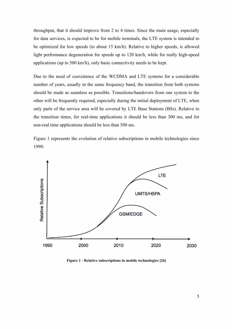
throughput, that it should improve from 2 to 4 times. Since the main usage, especially
for data services, is expected to be for mobile terminals, the LTE system is intended to
be optimized for low speeds (to about 15 km/h). Relative to higher speeds, is allowed
light performance degeneration for speeds up to 120 km/h, while for really high-speed
applications (up to 500 km/h), only basic connectivity needs to be kept.
Due to the need of coexistence of the WCDMA and LTE systems for a considerable
number of years, usually in the same frequency band, the transition from both systems
should be made as seamless as possible. Transitions/handovers from one system to the
other will be frequently required, especially during the initial deployment of LTE, when
only parts of the service area will be covered by LTE Base Stations (BSs). Relative to
the transition times, for real-time applications it should be less than 300 ms, and for
non-real time applications should be less than 500 ms.
Figure 1 represents the evolution of relative subscriptions in mobile technologies since
1990:
Figure 1 - Relative subscriptions in mobile technologies [26]

6
2.2. Network architecture
In principle, the LTE network structure is quite simple. Actually, it is simplified with
respect to the GSM and WCDMA structure: there is only a single type of access point,
the eNodeB (or Base Station, BS). Each BS can support one or more cells, providing the
following functionalities:
• Air interface communications and PHYsical layer (PHY) functions
• Radio resource allocation/scheduling
• Retransmission control
The X2 interface is the interface between different BSs. Important information is
exchanged through this interface for the coordination of transmissions in adjacent cells
(e.g. for reduction of the intercell interference). The S1 interface connects each BS to
the core network.
The LTE developed core network, called System Architecture Evolution (SAE) or
Enhanced Packet Core (EPC), is based on packet-switched transmission. It consists of a
Mobility Management Entity (MME), the serving gateway (connecting the network to
the RAN), and the packet data network gateway, which connects the network to the
Internet. In addition, the Home Subscriber Server is defined as a separate entity. The
core network complies the following functionalities:
• Subscriber management and charging
• Quality of service provisioning, and policy control of user data flows
• Connection to external networks
The network must also provide enough user security and privacy and network
protection against fraudulent use. Figure 2 represents the LTE network architecture:

7
Figure 2 - LTE network architecture [27]
2.3. Protocol architecture
In this section the LTE protocol architecture is explained. Figure 3 shows the different
protocol layer that structure the processing specified for LTE:
Figure 3 - LTE Protocol stack and main functions [25]

8
In figure 4 is illustrated a general overview of the LTE protocol architecture for the
downlink. Related to the LTE protocol structure of the uplink transmission, it is quite
similar to the downlink. However, with respect to multi-antenna transmission and
transport format selection there are some differences between them [1].
Prior to transmission over the radio interface, incoming IP packets are passed through
multiple protocol entities, enumerated bellow [1]:
Figure 4 - Overview of the LTE protocol architecture for downlink [1]
• Packet Data Convergence Protocol (PDCP) ciphers user and signaling traffic
over the radio interface. It ensures the integrity protection of the transmitted data
by protecting against attack scenarios. At the receiver side, PDCP performs the

9
deciphering and decompression operations. PDCP is also responsible of the IP
header compression. It is necessary to reduce the number of bits necessary to
transmit over the radio interface. The header compression is based on the ROHC
algorithm, used in WCDMA as well as other mobile-communication standards.
• Radio Link Control (RLC) is responsible for segmentation and reassembly,
retransmission handling, and in-sequence delivery for higher layers. The higher
layer packets need to be adapted to packet sizes that can be sent over the radio
interface. This protocol is located in the eNodeB since there is only a single type
of node in the LTE radio-access-network architecture. The RLC offers services
to the PDCP in the form of radio bearers.
• Medium Access Control (MAC) handles hybrid-ARQ retransmissions and uplink
and downlink scheduling. The scheduling functionality is located in the eNodeB,
which has one MAC entity per cell, for both uplink and downlink. The MAC
offers services to the RLC in the form of logical channels.
• Physical Layer (PHY) handles coding/decoding, modulation/demodulation,
multi-antenna mapping, and other physical layer functions. The physical layer
offers services to the MAC layer in the form of transport channels.
Now the RLC and MAC entities will be explained in more detail.
2.3.1. Radio Link Control
The Service Data Units (SDUs) are segmented and concatenated by the RLC into
available packets for transmission across the radio channel, named as Protocol Data
Units (PDUs). The PDU size can be adjusted dynamically, due to the dynamic changes
of the transmission data rates.
The RLC also ensures that all PDUs arrive at the receiver (RX) (and arrange for
retransmission if they do not), and delivers them to the PDCP in their correct order.
The scheduler decides the amount of data from the RLC SDU buffer should be selected
for transmission, and in order to create the RLC PDU, the SDUs are

10
segmented/concatenated. Hence, during a LTE transmission the PDU size varies
dynamically [2]. Figure 5 represents the RLC PDU creation.
It is important to note that the large PDU size resulted of high data rates means to a
smaller overhead. On the other hand, for low data rates is required a small PDU size.
Hence, as the LTE data rates may oscillate dynamically in a very large range, dynamic
PDU sizes are motivated for LTE.
Figure 5 - Radio Link Control PDU
2.3.2. Medium Access Control
The MAC layer provides HARQ (Hybrid Automatic Repeat Request) retransmissions
and is responsible for the functionality that is required for medium access, such as
scheduling operation and random access.
Logical channels and transport channels
The MAC communicates to the RLC in the form of logical channels, as mentioned
before. The type of information it carries defines a logical channel. These channels are
mainly classified into control channels (used for transmission of control and
configuration information necessary for operating an LTE system) and traffic channels
(used for the user data). Hence are enumerated the main logical channels:
• Broadcast Control Channel (BCCH): used for system control information
broadcasting from the network to all mobile terminals in a cell.

11
• Dedicated Control Channel (DCCH): used for transmission of control
information to/from a mobile terminal for single configuration.
• Paging Control Channel (PCCH): used for paging of mobile terminals whose
location on cell level is not known to the network.
• Multicast Control Channel (MCCH): used for transmission of control
information required for multiple reception.
• Dedicated Traffic Channel (DTCH): used for user data transmission to/from a
mobile terminal.
• Multicast Traffic Channel (MTCH): used for MBMS services downlink
transmission.
The transport channel is the format offered to the MAC layer from the physical layer. It
is defined by the way the information is transmitted over the network [1]. Data on a
transport channel is organized into transport blocks. The content of each transport block
is the set of bits collected in each Transmission Time Interval (TTI). The types specified
for transport channel are:
• Broadcast Channel (BCH): used for broadcasting the information on the BCCH
logical channel.
• Paging Channel (PCH): used for transmission of paging information on the
PCCH logical channel.
• Multicast Channel (MCH): used to support MBMS. It should be diffused
throughout the hole cell.
• Downlink Shared Channel (DL-SCH): used for downlink data transmission. It
supports hybrid ARQ, scheduling in the time and frequency domains, and spatial
multiplexing (MIMO).
• Uplink Shared Channel (UL-SCH): is the uplink counterpart to the DL-SCH.
Downlink scheduling
In the LTE radio access, time/frequency resources are shared between network users
during transmission dynamically both in uplink and downlink. The main target of the
12
scheduler is controlling the assignment of uplink and downlink resources. It is
important to know that downlink and uplink scheduling are separated in LTE, because it
means that schedule decisions of uplink and downlink transmission can be taken
independently of each other.
The downlink scheduler has to determine, in each 1 ms, which terminal(s) that are
waiting to receive transmission and the needed resources to reach this. It is possible to
have one DL-SCH per scheduled terminal, in which case each terminal is dynamically
mapped to a group of frequency resources. Thus, multiple terminals can be scheduled in
parallel. The scheduler is also responsible for selecting the modulation scheme, the
antenna mapping and modulation scheme. Moreover, the scheduler also controls the
data rate, so it decision will affect the RLC segmentation and MAC multiplexing [1].
Information about the downlink channel conditions, critical for channel-dependent
scheduling, is sent from the mobile terminal to the eNodeB via Channel Quality
Indicator (CQI). It includes information necessary to determine the right antenna
processing in case of spatial multiplexing.
Uplink scheduling
The uplink scheduler has to determine, for each 1 ms interval, which mobile terminals
(UEs) are to transmit data on their UL-SCH and on which uplink resources (similar to
the downlink scheduling basic function).
Thus, the time/frequency resource units are the shared resource controlled by the
eNodeB uplink scheduler. In addition, it is important to note that an already assigned
resource not fully utilized by a mobile terminal cannot be partially utilized by another
mobile terminal [1].
Another important feature in the uplink scheduling decision is that it is taken per mobile
terminal (and not per radio bearer). Thus, the terminal should select from which radio
bearer the data is taken.

13
Data flow
Figure 6 shows an example [1] of the flow of downlink data through all the protocol
layers, for a case with three IP packets (two on one radio bearer and one on another
radio bearer). The required information for deciphering in the terminal is included in the
PDCP header.
Figure 6 - Flow of downlink data through all the protocol layers [1]
The figure shows that each protocol sub-layer adds its own protocol header to the data
units, and how the RLC protocol performs concatenation and/or segmentation of the
PDCP SDUs and adds and RLC header. The MAC layer forwards the RLC PDUs, and
assembles them into a MAC SDU. Then attaches the MAC header to form a transport
block. Depending on the instantaneous data rate selected, the size of this transport block
will vary. After that, the physical layer adds a CRC (Cyclic Redundant Check) in order
to detect errors. Besides that, this layer performs modulation and coding and transmits
the signal over the network. The next chapter provides more information about this
layer.

14

15
3. LTE Physical Layer
“The physical layer is responsible for coding, physical-layer hybrid-ARQ processing,
modulation, multi-antenna processing, and mapping of the signal to the appropriate
physical time–frequency resources. It also handles mapping of transport channels to
physical channels” [2].
3.1. LTE frame structure
LTE employs OFDM for downlink data transmission and SC-FDMA for uplink
transmission. In the next section both modulation techniques will be approached.
3.1.1. OFDMA
OFDMA is considered the main multiplexing scheme in the LTE downlink. This is a
technology that allows multiple access by dividing the channel into a group of
orthogonal subcarriers, scattered in other sub-groups according to the each user needs.
Relative to the resource scheduling, OFDMA added complexity; however, its
improvements result OFDMA to be much better than the current schemes in terms of
network latency and efficiency [5].
As mentioned before, the main key in OFDMA is the signal orthogonality. This allows
mixing several signals in transmission and then separating it in reception without any
interference between them.
In OFDMA, users are allocated a specific number of subcarriers for a predetermined
amount of time. These are named as physical Resource Blocks (RBs). The eNodeB
scheduler is the responsible for handling the RBs allocations.
In LTE, the time is divided into entities [3]:

16
• A radio frame, which has duration of 10 ms, is the fundamental time unit of LTE
transmission.
• Each radio frame is divided into 10 sub-frames of 1 ms long. These sub-frames
are the most LTE processing fundamental time unit.
• Each sub-frame is consisted of two slots (each being 0.5 ms long).
• Each slot is consisted of 6/7 symbols.
We can show this hierarchy in figure 7:
Figure 7 - LTE Generic Frame Structure [5]
Depending on the overall transmission bandwidth of the system, it will be a different
number of subcarriers available to transmit/receive. The transmitted downlink signal is
consisted of NUL subcarriers for duration of Nsymb OFDM symbols. A resource grid can
represent it, like it is shown in figure 8. The resource element represents a single
subcarrier for one symbol period within the grid.

17
Figure 8 - Resource blocks for uplink and downlink
Figure 9 represents cleaner the relationship between RBs y resource elements:
Figure 9 - LTE resource block vs. resource element [2]
As described before, groups of 12 adjacent subcarriers are grouped together on a slot-
by-slot basis to form resource blocks (RBs).

18
3.1.2. SC-FDMA
LTE uplinks requirements are different from downlink, due to the different nature of the
UE terminals. For example, power consumption is one of the most important topics
during uplink transmission. Due to the loss of efficiency associated with OFDMA
signaling, Single Carrier – Frequency Domain Multiple Access (SC-FDMA) is well
suited to the LTE uplink requirements.
SC-FDMA presents the same advantages than OFDMA. However, the SC-FDMA
signal represented by the subcarrier is single, because the SC-FDMA subcarriers are not
independently modulated (unlike OFDMA). As a result, the Peak-to Average Power
Ratio (PAPR) is lower than for OFDM transmissions [5].
Due to the project approach is focused on the downlink data transmission, the uplink
scheduler won’t be mentioned in greater detail.

19
3.2. Multi-Antenna techniques
In order to reach the aggressive LTE performance targets, the main key performance of
this technology is the use of more than one single antenna during transmission.
Multiple antennas can be used in different ways to achieve different aims:
• Multiple antennas at the transmitter and/or the receiver can be used for receive
diversity.
• Multiple transmit antennas at the base station can be used for transmit diversity
and different types of beam forming.
• Spatial multiplexing, also referred to as MIMO (Multiple Input – Multiple
Output), using multiple antennas at both the transmitter and receiver.
The different multi-antenna techniques are beneficial in distinct scenarios, where
multiple antennas at the transmitter side should be used to increase the SNR (Signal to
Noise Ratio) by means of beam forming [1].
3.2.1. Multiple transmit antennas
By applying multiple antennas at the transmitter side, diversity and beam forming can
be achieved. The use of multiple transmit antennas is mainly of interest for the
downlink (at the base station). In this case, the use of multiple transmit antennas
provides a chance for diversity and beam forming without the need for additional
receive antennas and corresponding additional complexity at the terminal [2].
Transmit-Antenna Diversity
If there is no knowledge available of the downlink channels of the transmit antennas at
the transmitter, this technique cannot provide beam forming but only diversity. In this
case, there should be low mutual correlation between the channels of the different
antennas. This technique can be shown in figure 10.

20
Figure 10 - Diversity channel with an M-element transmit antenna array [29]
Transmitter-Side Beam Forming
Multiple transmit antennas can also provide beam forming in case that there is some
knowledge available of the downlink channels of the different transmit at the transmitter
side.
A small inter-antenna distance configuration means generally high mutual correlation.
Thus, in this case the channels between a receiver and the different transmit antennas
are basically the same. In figure 11 it can be shown.
Thus, applying different phase shifts to the signals to be transmitted on the transmit
antennas allows handle the transmission beam.
Figure 11 - Classical beam-forming with high mutual antennas correlation [2]
3.2.2. Spatial multiplexing
In the scenario of multiple antennas at the transmitter and the receiver, also emerges the
possibility for the spatial multiplexing. It makes a more efficient use of the Signal-to-

21
Noise and Signal to Interference ratios and allows higher transmission data rates over
the LTE radio interface [2].
Under certain conditions [2], attempting to avoid the saturation in the data rates is
possible to increase the channel capacity with the number of antennas.
Closed-Loop Spatial Multiplexing
In closed-loop spatial multiplexing, the codewords (the parsed output of the decoders)
are mapped onto the layers by the next procedure [3]:
• If the number of codewords equals the number of layers, then each layer simply
contains the symbols from one codeword.
• If there is one codeword and two layers, then the symbols of the codeword are
alternatingly assigned to layer 1 and layer 2.
• If there are 2 codewords and 4 layers, then symbols from codeword 1 are
alternatingly assigned to layer 1 and 2, while symbols from codeword 2 are
alternatingly assigned to layer 3 and 4.
Open-Loop Spatial Multiplexing
In the case that is not available a feedback of the desired beam forming, this
multiplexing can be used [3].
Downlink Multi-User MIMO
MIMO (Multiple Input – Multiple Output) intends to exploit the spatial multiplexing by
suppressing the interference between the different layers. MU-MIMO (Multi-User
MIMO) is a MIMO extension. SU-MIMO (Single User MIMO) attends to improve the
link between base station and user features, while MU-MIMO pretends the coexistence

22
of several different users sharing the same frequency range. For this purpose, MU-
MIMO attempts to exploit a possible spatial decouple between the data flow transmitted
and each user for, if it is possible, reach better data rates and efficiency.
Summary, SU-MIMO aims to improve the link capacity while MU-MIMO pretends to
increase the cell capacity. Figure 12 represents a downlink transmission from a cell to
one or more UEs in MU-MIMO configuration.
Figure 12 - Downlink transmission in MU-MIMO configuration [28]

23
4. 3D Video transmissions
4.1. State-of-art
The goal of any multimedia delivery system is to ensure the best video end quality
possible, and to achieve this purpose the video created has not to be degraded when it is
delivered to the consumer.
Nowadays, 3D video is revolutionizing the audiovisual industry due to the immersion
sensation that it produces. Current generation of digital video carries revolutionary
aspects as the emergence of new data types in the media.
Many applications are adopting 3D video, and this has resulted in a considerable impact
on the market. The need for extending the visual sensation to the 3D (three-dimension)
is believed to grow, thus it brings the nearly development and distribution of contents,
3D video processing capable devices and 3D video encoding/decoding standards.
Indeed, two main applications refer to 3D video: 3DTV and FVV (Free Viewpoint
Video).
3DTV application reaches the 3D perception by fusing two displayed images (one for
each eye but from two slightly different viewpoints). It makes the human vision system
to assess depth.
In FVV application the user is free to select the desired viewpoint of the displayed
scene, thus this furnishes interactivity.
Nowadays, three-dimensional (3D) video representation is one of the technologies that
are having greater popularity. A 3D video provides the illusion on the depth perception,
thus adding an increased degree of realism to the human eye reception. It gives in fact a
value added to the consumer experience.
Due to this reason, 3D video is expected to be the most adopted in the next years in
many application fields (e.g. medicine, entertainment, etc.). Actually, recent studies
pointed that 3D video is one of the most active research topic nowadays.

24
4.2. 3D video system
Depending on the targeted application, different representations are available for 3D
video and should be rightly chosen.
A 3D content can be provided by a 3D video system in different forms, depending on
the input source, the desired quality level, the type of acquisition and scene geometry,
the kind of application and the bandwidth [8].
A 3D video system is subdivided into four main groups, as represents figure 13:
Figure 13 - Structure of an end-to-end 3D video system
4.2.1. 3D content creation
This block is the responsible for providing the data that will be used to set up the 3D
video. Firstly the data is captured. Then, it is sent to post-processing, where some
algorithms are applied to improve accuracy. Once the data is processed, it is sent to the
3D reconstruction phase, that has the task of creating the data transmitted during the 3D
video representation. For more details, see [9].
4.2.2. 3D representation
There are different types of 3D scene representation, depending on the target application
and capture devices. They can be classified as in image- and geometry-based formats
and also hybrid representation based on the depth maps, which is a combination of
image and geometric aspects.
3D content creation -‐ Capture -‐ Post-‐processing -‐ 3D Reconstruction
3D representation
Delivery -‐ Coding -‐ Transmission -‐ Decoding
Visualization -‐ Rendering -‐ 3D Displays

25
Image-based representation
The most widespread approach makes use of a couple of cameras that capture
separately, like human eyes, left and right images. It is a stereoscopic video format
composed by two video signals, one for each eye. It is the format used by movie
theaters and current 3DTV for home entertainment. The two video signals can be
encoded by performing temporal or spatial interleaving. Then, a single frame is formed
by the right and left eye images [9]. It can be shown in figure 14. The balls represent the
eyes (right and left) and the “blue box” forms the video screen.
Figure 14 - Image-based representation
Geometry-based representation
Is the extension from 2D to 3D, where the data is represented by voxels instead of
pixels. This kind of representation is mainly used in computer-generated graphics for
gaming or medical purposes.
V V
R
L
R
L
Screen

26
Depth maps-based representation
A representation of a point in 3D-space in this case consists in a three-dimensional
vector. The depth expresses, in fact, this third coordinate.
The most important development in 3D video is the depth perception, compared to the
conventional (2D) video. However, it has a disadvantage: its transmission requires the
additional information to be sent as well as more bandwidth and a lower loss probability
[10].
A depth map is a gray scale image describing the depth position of the objects using a
gray scale typically ranging from white (the closest to the display plane) to black (the
farest from the display plane). In it, the distance from the sensor to a visible point at the
scene is represented by each pixel.
There are different coding and transmissions arrangements, from the simple video-plus
depth simulcast to the complex multiview-plus-depth format (MVD). These two
formats will be mentioned in this work.
The video-plus-depth (V+D) format consists in a 2D conventional color video (texture)
and an associated depth-map. Each of these depth-images stores depth information,
resulting from an 8-bit gray scale quantization. These 256 gray scale values can create a
smooth gradient of depth within the image. In order to reconstruct the second view sub-
frame, the decoder will use the frames and their depth-map. This is carried out by using
Depth Image-based Rendering (DIBR) techniques (see [8] for more details).
Figure 15 shows the DIBR procedure:

27
Figure 15 - DIBR procedure [12]
The multiview-plus-depth format (MVD) can be considered as a multiple 2D videos
used with their associated depth video, providing more V+D streams. It requires a
complex procedure.
Figure 16 represents a MVD system:
Figure 16 - MVD System [15]

28
The depth-based representation is widely used in research, standardization and industry
[13], because it comprises a number of advantages [11]:
• According to personal preferences of the viewer, it offers the possibility of a
customized 3D experience, with either stereoscopic or autostereoscopic displays.
• Efficient compression (high compressed ratio): noise-free depth maps can be
represented with only up to 25% of the texture bitrate, making 3D video format
based on texture complemented with depth information compatible with the
current transmission bandwidth.
• Ability to render virtual views.
4.2.3. Delivery
3D video coding, transmission and decoding are carried out in this stage. Before being
transmitted over the network, it is often necessary to compress the 3D video. It is
important to know that the highest compression efficiency is one that removes less
important information from the video stream.
The H.264/AVC (Advance Video Coding) compression standard with Scalable Video
Coding (SVC) extensions is one of most extended compression standard (actually, there
is another one better, HEVC), and it is highly used, so in this work only this video
codec will be mentioned. It is shown that H.264 increases coding efficiency by
approximately 50% compared to previous MPEG standards [14]. LTE networks need to
support mobile devices with different displays resolution requirements like small
resolution mobile phones and high-resolution laptops. Recognizing this trend, the SVC
extension of H.264 allows efficient temporal, spatial and quality scalabilities.
4.2.4. Visualization
This building block is the most important to the end user, because it takes care of the
visualization of the 3D video. Its stages are rendering and 3D displays.
29
The rendering stage employs algorithms to convert the data stored at the representation
format. Due to the FVP functionalities and 3D displays needs, the rendering stage
focuses on the view synthesis methods.
3D displays are responsible for depth perception of 3D videos. Since 3D media became
more accessible to home users, these are in constant development. Recent studies
predict that in 2015 more than 30% of all high definition panels at home will have 3D
capabilities [9].

30
4.3. Objective quality metrics of 3D video
In terms of quality control, performance evaluation and resource allocation, is critical to
have a good objective video quality assessment (VQA) in a 3D video transmission
system.
Visual applications have greatly evolved especially during last years. This has led to a
large growth of the demand for video quality assessment technologies [19].
Until now the objective and subjective quality metrics of 2D video has been a constant
research topic. However, since the 3D technologies are emerging, it is required new
quality assessments and methodologies due to the critical differences in the human
visual perception and the typical distortions of the 3D video content.
Due to the availability of several image and 2D video public databases, with common or
different features (e.g. spatial resolution, severity of distortions, etc.), to perform
realistic comparisons between different objective quality metrics is very difficult.
The work [11] describes the state-of-the art quality metrics for 3D image and video, and
the overall conclusion is that it is very difficult (or even impossible) to compare the
performance of two different 3D quality evaluation algorithms; every quality metric has
its pros, cons, objectives and application scope.
Objective metric quality measures have to provide an indication of quality close to the
subjective indication given by the observers. The Pearson Linear Correlation
Coefficient (PLCC) is the most used metric in order to evaluate the performance of
objective video quality model. For N data pairs (𝑥! ,𝑦!), with 𝑥 and 𝑦 being the means
of the respective data sets, the PLCC is given by:
(1) 𝑃𝐿𝐶𝐶 = (𝑥𝑖−𝑥)(𝑦𝑖−𝑦)𝑁𝑖=1
(𝑥𝑖−𝑥)2𝑁
𝑖=1 ∗ (𝑥𝑖−𝑥)2𝑁
𝑖=1
∈ [−1,1]
Table 2 shows the PLCC performance comparison of VQA algorithms:

31
Database VQEG IRCCyN EPFL-PoliMI LIVE
PSNR 0.7683 0.4160 0.7351 0.5621
SSIM [20] 0.8215 0.5012 0.6781 0.5444
VQM [21] 0.8170 0.4850 0.8434 0.7236
MOVIE [22] 0.8210 0.4850 0.9210 0.8116
Yu et al. [23] 0.8170 0.7680 0.9470 0.8450
3D-SSIM [19] 0.8403 0.8194 0.9621 0.8353
Table 2 - PLCC performance comparison of VQA algorithms [19]
In the next section the SSIM (Structural Similarity Index) will be introduced.
4.3.1. Media-layer FR image quality models
There are several models to evaluate the quality of an image reference to the original,
but the two most widely known are the Peak Signal to Noise Ratio (PSNR) and the
Structural Similarity Index (SSIM) [11].
PSNR can be defined as:
(2) 𝑃𝑆𝑁𝑅 = 10 𝑙𝑜𝑔!"(2𝑛−1)
2
𝑀𝑆𝐸 , with 𝑀𝑆𝐸 = 1𝑁 (𝑥𝑖 − 𝑦𝑖)2𝑁
𝑖=1
where 𝑁 is the number of pixels of the original image 𝒙 and the distorted image 𝑦, and
𝑛 is the number of bits per pixel (typically 8). For application-generic purposes, since
the MSE does not reflect the way that human visual systems perceive image
degradation, this measure has poor correlation with perceived image quality.
On the other hand, to extract structural information from visual scenes, the HVS (human
visual systems) is highly adapted. However, its disadvantage is that, given the large
volume of video data being transmitted everyday, they are extremely slow and
expensive.
A measurement of structural similarity should provide a good approximation to
perceptual image quality. For this purpose, the SSIM evaluates image similarity based
on three factors computed from the two images being compared [11]: luminance l(x,y),
contrast c(x,y) and structure s(x,y), defined as:

32
(3) 𝑙 𝑥,𝑦 = 2𝜇𝑥𝜇𝑦+𝐶1𝜇𝑥2+𝜇𝑦2+𝐶1
, 𝑐 𝑥,𝑦 = 2𝜎𝑥𝜎𝑦+𝐶2𝜎𝑥2+𝜎𝑦2+𝐶2
, 𝑠 𝑥,𝑦 = 𝜎𝑥𝑦+𝐶3𝜎𝑥𝜎𝑦+𝐶3
where x and y are the reference and the distorted image luminance pixel values, µ and σ
represent the mean and the standard deviation, and C1, C2 and C3 are small constants
added for numerical stability. By combining these three factors, the overall similarity
measure is inferred:
(4) 𝑆𝑆𝐼𝑀 𝑥,𝑦 = 𝑙 𝑥,𝑦 ! · 𝑐 𝑥,𝑦 ! · 𝑠 𝑥,𝑦 ! , 𝛼,𝛽, 𝛾} > 0
The score provided by the SSIM ranges between 0 and 1; the closer to 1, the higher the
similarity of the distorted image to the reference image and so in this context the better
the quality of the image. In this work this quality model will be the used.

33
5. Methods, tools and simulated scenario
In this work was performed an evaluation of the effect of losses of compressed 3D
video transmitted over an LTE system.
For this purpose, the “LTE-A System Level Simulator” of the University of Wien was
the main tool used in order to obtain the frame-by-frame Block Error Rate (BLER)
values experienced by different UEs.
Thus, using this simulator is possible to obtain the BLER of each transmission time
interval (TTI) during the simulation. The selected UE describes a path, and every on
millisecond his BLER (Block Error Rate) will be stored into a trace. Figure 17 describes
this procedure:
Figure 17 - Simulated scenario
In this chapter an overview of this simulator will be described.
5.1. The University of Vienna System Level LTE Simulator
In order to evaluate the performance of new mobile network technologies, system level
simulations are crucial. They aim at determining whether, and at which level predicted
link level gains impact network performance [16].
eNodeB
UE position
BLER

34
This simulator evaluates the performance of the Downlink Shared Channel of LTE
SISO and MIMO networks using Open Loop Spatial Multiplexing and Transmission
Diversity transmit modes (mentioned before in this work).
In addition to the System-Level simulator, there is another LTE simulator: the “LTE
Link-Level Simulator” [17]. Using both simulators it is possible to obtain results where
the results of physical and link-level are isolated from each one and is easier to
investigate the performance of the network.
After studying both simulators, the System-Level was chosen because using the Link-
Level simulator is not possible to reflect the effects of issues, such as cell planning,
scheduling, or interference.
Figure 18 shows the schematic block diagram of the simulator:
Figure 18 - Schematic block diagram of the simulator [16]
The simulator outputs traces containing throughput and error rates, from which their
distributions can be computed.

35
The link measurement model is focused on the measured link quality used for resource
allocation and link adaptation. Moreover, the link performance model is responsible for
the determination of the Block Error Ratio (BLER) at the receiver given a certain
resource allocation and Modulation and Coding Scheme (MCS).
For LTE are defined different MCS, driven by 15 Channel Quality Indicator (CQI)
values. This CQI values use coding rates between 1/13 and 1 combined with 4-QAM,
16-QAM and 64-QAM modulations. (In this work only 16-QAM was used).
Figure 19 represents the CQI vs BLER curves on the left, and the CQI obtained from
the 10% BLER points (right).
Figure 19 - CQI vs. BLER curves (left) and CQI from the 10% BLER points (right) [18]
5.1.1. Using the simulator
The objetive of this part of the work is to obtain the BLER traces of a specific UE. The
configuration parameters are in table 3. The reasons of choosing this parameters is
described in sections 6 and 7.
PARAMETER VALUE
Simulation length 30 s
Network details -‐ 7 macro cells (trisector each one) with radius equal to

36
0.5 km;
-‐ number of user in each cell: chosen in the range [5, 30];
-‐ speeds chosen between 5 km/h, 36 km/h and 72 km/h;
-‐ mobility model: straigh model, random direction
Physical detail
-‐ Carrier Frequency: 2 GHz;
-‐ Bandwidth for the DL: 10 MHz;
-‐ Antenna system: MIMO 2x1 with Closed Loop Spatial
Multiplexing;
-‐ Modulation Scheme: 16-QAM;
-‐ Propagation loss model: urban;
-‐ eNodeB power transmitted: 40 dBm;
Protocol Overhead
-‐ RTP/UDP/IP with ROHC compression: 3 bytes;
-‐ MAC and RLC: 5 bytes;
-‐ PDCP: 2 bytes
-‐ CRC: 3 bytes
-‐ L1/L2: 3 symbols;
Table 3 - Configuration parameters of the System Simulator
The network is represented in figure 20 (corresponded to 30 UEs per eNodeB):
Figure 20 - UEs network configured (30 UEs per eNodeB)

37
Where the blue points represents the initial position of the UEs at the begin of the
simulation. The red point represents the initial position of the studied UE. The positions
of the trisector eNodeBs (base stations) are represented in figure 21:
Figure 21 - Base station positions
The positions of the studied UE are represented in the next three figures, one for each
speed. The red trace represents the evolution of the studied UE position during the
simulation.
Figure 22 - UE positions for 5km/h

38
Figure 23 - UE position for 36km/h
Figure 24 - UE positions for 72km/h
It can be appreciated in the figures that the studied UE direction is 233°.

39
5.2. Evaluated scenarios
It could be represented a diagram of the evaluated scenario in this work:
Figure 25 - Diagram of the evaluated scenario
Thus, after obtaining the Block Error Rate for the UE during the simulation, the BLER
trace was converted to a packet level error trace (binary error trace). For this purpose,
firstly the BLER trace (with its respective block length –in this case, 6-) is converted to
a Bernoulli sequence of packet loss events. The next step is, given a file of lengths (in
bits) of compressed 3D video file and the Bernoulli sequence mentioned, create a binary
sequence of packet level error traces.
eNodeB
UE position
BLER
Packet-level error traces
Corrupted 3D video encoded
Error-concealment capable video decoder
Quality of Experience Calculator
RESULTS

40
The Bernoulli sequence provides a sequence of packet error trace. Thus, given the
system-layer transport block sizes (as mentioned, it changes dynamically) and the
lengths of the 3D video file packets, it is possible to know the amount of system-layer
packets that forming each 3D video file packet. Figure 26 shows an example:
Once obtained this information, based on the Bernoulli sequence, in order to create the
packet level error trace the decision was basically establish an error packet if this packet
had any loss.
Figure 27 shows the structure of this conversion:
Figure 27 - Block Diagram of the BLER conversion
The corrupted encoded video stream will be decoded using an error-concealment
capable video decoder and the decoded/recovered video quality (QoE) will be estimated
based on the Structural Similarity Index of the recovered video. This last block is not in
the scope of this work; please refer to [11] for further information.
3D video traces
System-layer packets
1 2 3 4 5
1 2
BLER Bernoulli sequence
Bernoulli Function
3D Video Lengths
Packet level error trace
Figure 26 - System-layer packets and 3D video traces

41
6. Experiments and results
As mentioned before, three different user speeds were simulated: 5 km/h (1.38 m/s), 36
km/h (10 m/s) and 72 km/h (20 m/s). The main purpose of using this values is that 5
km/h is the minimum user speed available in the simulator. The other two values are
realistic in an urban environment (e.g. user travelling in a car).
Four different 3D video coded files where corrupted to obtain the results: kendo,
balloons, lovebird and newspaper. The analysis of this files is out of the scope of this
work, in [11] it is highly analyzed. Table 4 shows the encoder setting parameters of the
videos used:
3D video
(spatial resolution)
Bitrate
(kb/s)
Bit budget
(%)
Average
PSNR (dB)
Balloons (1024x768)
Tex. 1095 84.8 % 41.41
Dep. 196 15.2 % 39.47
Kendo (1024x768)
Tex. 1173 79.6 % 42.45
Dep. 300 20.4 % 38.40
Lovebird (1024x768)
Tex. 825 89 % 39.17
Dep. 102 11 % 42.32
Newspaper (1024x768)
Tex. 935 85.5 % 39.28
Dep. 150 14.5 % 39.08
Table 4 - Encoder setting parameters of the videos used
Where the bit budget column represents the amount of space in the encoded packet
occupied by the texture packet or the depth packet, respectively.
In order to understand better the results, first the results of the intermediate stage (the
simulator output results) will be shown.

42
6.1. Simulator output results
6.1.1. Balloons
Figure 28 - PLR results for Balloons
6.1.2. Kendo
Figure 29 - PLR results for Kendo

43
6.1.3. Lovebird
Figure 30 - PLR results for Lovebird
6.1.4. Newspaper
Figure 31 - PLR results for Newspaper

44
6.1.5. Overview
The next 4 tables show the numeric data of the PLR, one for each video file.
Balloons
UEs per eNodeB
UE speed 5 10 15 20 25 30
5 km/h 7.2291 7.2916 9.2083 11.2916 15.1875 18.6875
36 km/h 9.3541 10.7083 10.7083 14.2708 18.2291 28.8958
72 km/h 9.875 12.2708 13.7916 15.3750 21.7916 32.5208
Table 5 - PLR results from Balloons
Kendo
UEs per eNodeB
UE speed 5 10 15 20 25 30
5 km/h 8.4166 9.6250 11.3968 11.4583 16.7708 20.9166
36 km/h 9.8750 11.2291 13.6458 16.4375 22.6458 27.7708
72 km/h 12.896 14.7916 15.9375 21.1041 24.2708 31.3750
Table 6 - PLR results from Kendo
Lovebird
UEs per eNodeB
UE speed 5 10 15 20 25 30
5 km/h 4.4010 5.9375 8.0468 10.8333 12.6562 13.2292
36 km/h 6.2500 6.8750 9.0104 11.4323 14.1146 22.6458
72 km/h 6.7448 7.7083 10.0264 11.6666 15.3385 23.1250
Table 7 - PLR results from Lovebird

45
Newspaper
UEs per eNodeB
UE speed 5 10 15 20 25 30
5 km/h 6.2916 7.1666 8.3125 10.8958 14.5833 16.4375
36 km/h 6.8750 8.6259 12.0625 13.6458 16.1666 27.5120
72 km/h 8.0625 10.4792 12.8333 14.4166 22.4791 31.6666
Table 8 - PLR results from Newspaper
After being shown the results of the intermediate stage, the output final results will be
given in the next subsection, as well as the analysis of them.

46
6.2. QoE results
After obtaining the PLR results and extract the Block Error Rate, the BLER sequences
were converted to packet level error traces and used to corrupt the 3D codec video files.
The QoE results of this files are shown in the next four figures:
6.2.1. Balloons
Figure 32 - QoE results for Balloons
6.2.2. Kendo
Figure 33 - QoE results for Kendo

47
6.2.3. Lovebird
Figure 34 - QoE results for Lovebird
6.2.4. Newspaper
Figure 35 - QoE results for Newspaper

48
6.2.5. Overview
The next table shows the numeric data of the Structural Similarity Index (SSIM).
Balloons
UEs per eNodeB
UE speed 5 10 15 20 25 30
5 km/h 0,8841 0,8606 0,8593 0,8581 0,8362 0,8284
36 km/h 0,8820 0,8587 0,8417 0,8336 0,8264 0,8256
72 km/h 0,8581 0,8403 0,8322 0,8253 0,8217 0,8146
Table 9 - SSIM results from Balloons
Kendo
UEs per eNodeB
UE speed 5 10 15 20 25 30
5 km/h 0,8563 0,8564 0,8455 0,8391 0,8266 0,7904
36 km/h 0,8525 0,8479 0,8449 0,8269 0,8019 0,7852
72 km/h 0,8424 0,8262 0,8270 0,8059 0,7909 0,7485
Table 10 - SSIM results from Kendo
Lovebird
UEs per eNodeB
UE speed 5 10 15 20 25 30
5 km/h 0,8354 0,8092 0,7785 0,7768 0,7752 0,7313
36 km/h 0,8092 0,78628 0,77705 0,7754 0,7401 0,6868
72 km/h 0,7972 0,7754 0,75707 0,7386 0,6965 0,6855
Table 11 - SSIM results from Lovebird

49
Newspaper
UEs per eNodeB
UE speed 5 10 15 20 25 30
5 km/h 0,8129 0,7841 0,7738 0,7652 0,7452 0,7070
36 km/h 0,7655 0,7651 0,7616 0,7392 0,7106 0,7013
72 km/h 0,7647 0,7520 0,7403 0,7120 0,7098 0,6605
Table 12 - SSIM results from Newspaper
6.3. Analysis of the results
The simulation results are consistent with expectations. It can be seen that the Packet
Loss Ratio (PLR) increases with user speed. As mentioned before in this work, LTE is
optimized for low speeds (to about 15 km/h). At higher speeds, due to the multipath
propagation, interference and handover delay effects, the communication will suffer
losses.
Thus, if the user is walking (around 5 km/h), the LTE transmission shouldn’t suffer too
many losses (in this case, PLR values are situated between 4% and 12%). On the other
hand, if the user speed is incremented, the LTE transmission will start to experience
losses in the link, with a PLR ranging between 13% and 32%.
Moreover, relative to network users density, the PLR increases also users density. It is
also expected: if there are more active users in the network, the link level error will
increase.
In terms of Structural Similarity Index (SSIM), it takes places the opposite of PLR
evolution. This is also consistent with expectations: if the user speed increases, the
SSIM will be decreased; and if the network user density tends to grow, the SSIM will
fall.

50

51
7. Conclusion
In this thesis, the main goal was to perform the simulation of losses of compressed 3D
video transmitted over an LTE system.
The first step, study the simulator capabilities and evaluate its behavior into our
problem, was successfully achieved. Firstly it was tested the Link-Level simulator, but
finally it was discarded because it didn’t comply with the main purpose. After
simulating different scenarios, finally the System-Level was used. It is critical to
establish a realistic simulated scenario, so the first issue to overcome was to decide the
simulation length, and the transmit mode in LTE. The simulation length, after studying
deeply the simulator, was fixed in 30 seconds, and the transmit mode in MIMO 2x1
(mentioned before), because MIMO is the main transmit mode in LTE nowadays.
It’s important to take account the limits of the 3D video corrupter, because it can’t be
able to analyze data frames with bandwidth upper to 1.4 MHz and with modulations
higher than 16-QAM. Therefore, these limits were the simulation limits.
Then, the output results of the simulations were studied. Since it was found that the
output frames didn’t provide the packet level error traces, it was performed a program in
order to convert this BLER sequences to packet level error traces (mentioned before in
this work).
Finally it was obtained the packet level error traces of a single UE during the
simulation, so the main goal of this thesis was successfully achieved.
The best QoE results are those corresponding to the speed of 5 kilometers per hour and
5 users per base station, and the worst ones are those corresponding to the speed of 72
kilometers per hour and 30 users per base station. The network congestion and the user
speed cause losses in the LTE transmission, as mentioned before.
The observed results show the dependency of the QoE on the increase of the number of
LTE users and user speed. As a final conclusion, it can be argued that the work
presented complies with the initial objectives.

52
It’s difficult to evaluate the QoE of a 3D video in a LTE transmission objectively.
Furthermore, the quality references are continuously changing due to the advances of
technology. However, these simulations can help to infer the relationship between the
system configurations (user densities, user velocities) and the achievable QoE.
As a future work, it could be suggested a study based on the comparison between the
encoder setting parameters of the four 3D video coded files and the QoE obtained
during the simulation in this dissertation.
The evolution in 3D technologies and the next LTE release will certainly cause an
important growth in the use of these technologies in mobile networks. The next step in
video technologies is the evolution for 2D video to 3D video, because it increases the
user experience.
Therefore, the task of the engineering will be developing the 3D technologies in mobile
networks, because the demand is continually growing.

53
References
[1] E. Dahlman, S. Parkvall, J. Sköld and P. Beming, “3G Evolution: HSPA and
LTE for Mobile Broadband”, Elsevier, 2007.
[2] E. Dahlman, S. Parkvall and J. Sköld, “4G LTE/LTE-Advanced for Mobile
Broadband”, Elsevier, 2011.
[3] A. F. Molisch, “Wireless Communications”, 2nd Edition, 2011.
[4] Campus Sur de la Universidad Politécnica de Madrid, “Capa Física y
Planificación en LTE”, in LTE: Long Term Evolution, 2013.
[5] J. Zyren, “Overview of the 3GPP Long Term Evolution Physical Layer”,
Freescale Semiconductor, 2007.
[6] T. Kim, J. Kang, S. Lee and A. C. Bovik, “Multimodal Interactive Continuous
Scoring of Subjective 3D Video Quality of Experience”, IEEE Transactions on
Multimedia, vol. 16, no.2, Feb. 2014.
[7] S. Singh, O. Oyman, A. Papathanassiou, D. Chatterjee and J.G. Andrews,
“Video capacity and QoE enhancements over LTE”, IEEE International
Conference on Communications (ICC), Jun. 2012.
[8] J. Gautier, E. Bosc and L. Morin, “Representation and coding of 3D video data”,
in Schémas Perceptuels et Codage video 2D et 3D, Feb. 2011.
[9] L. Rocha and L. Gonçalves, “An Overview of Three-Dimensional Videos: 3D
Content Creation, 3D Representation and Visualization”, Intech, 2012.
[10] G. Piuro, C. Ceglie, D. Striccoli and P. Camarda, “3D video transmissions over
LTE: a performance evaluation”, IEEE EUROCON Conference, Jul. 2013.
[11] J. R. Simões Soares, “Quality Evaluation of 3D Video Subject to Transmission
Channel Impairments”, Dissertação de Mestrado, Sept. 2013.
[12] M. Lee, J. Lee and H. Lee, “Perceptual Watermarking for 3D Stereoscopic
Video using Depth Information”, 2011 Seventh International Conference on
Intelligent Information Hiding and Multimedia Signal Processing, Sept. 2011.
[13] C. T. Hewage and M. G. Martini, “Quality evaluation for real-time 3D video
services”, IEEE International Conference on Multimedia and Expo (ICME), Jul.
2011.

54
[14] R. Radhakrishnan and A. Nayak, “Cross layer design for efficient video
streaming over LTE using scalable video coding”, IEEE International
Conference on Communications (ICC), Jun. 2012.
[15] Daribo, “An interactive depth-based multi-view system for 3DTV”, Keio
University, Oct. 2012.
[16] C. Ikuno, M. Wrulich and M. Rupp, “System Level Simulation of LTE
networks”, IEEE 71st Vehicular Technology Conference, May. 2010.
[17] C. Mehlführer, J. C. Ikuno, M. Simko, S. Schwarz, M. Wrulich and M. Rupp,
“The Vienna LTE Simulators – Enabling Reproducibility in Wireless
Communications Research”, EURASIP Journal on Advances in Signal
Processing, 2011.
[18] C. Ikuno, “Vienna LTE Simulators: System Level Simulator Documentation,
v1.7r1119”, Institute of Telecommunications of Vienna University of
Technology, March 2013.
[19] Zeng and Z. Wang, “3D-SSIM for Video Quality Assessment”, IEEE
International Conference on Image Processing (ICIP12), Sept. 2012.
[20] Z. Wang, A. C. Bovik, H. R. Sheikh, and E. P. Simoncelli, “Image quality
assessment: From error visibility to structural similarity,” IEEE Trans. Image
Processing, vol. 13, no. 4, pp. 600–612, April 2004.
[21] H. Pinson and S. Wolf, “A new standardized method for objectively measuring
video quality,” IEEE Trans. Broadcasting, vol. 50, no. 3, pp. 312–322,
September 2004.
[22] K. Seshadrinathan and A.C. Bovik, “Motion tuned spatiotemporal quality
assessment of natural videos,” IEEE Trans. Image Processing, vol. 19, no. 2, pp.
335–350, Feb. 2010.
[23] J. You, J. Korhonen, A. Perkis, and T. Ebrahimi, “Balancing attended and global
stimuli in perceived video quality assessment,” IEEE Trans. Multimedia, vol.
13, no. 6, pp. 1269–1285, Dec. 2011.
[24] M. Nasralla, O.Ogneoski and M.G. Martini, “Bandwidth Scalability and
Efficient 2D and 3D Video Transmission over LTE Networks”, IEEE
International Conference of Communications”, 2013.
[25] M. Sauter, “From GSM to LTE: an introduction to mobile networks and mobile
broadband”, WirelessMoves, Wiley Ed., 2011.
55
[26] P. Rysavy, “Transition to 4G: 3GPP Broadband Evolution to IMT-Advanced
(4G)”, Rysavy Research, 2010.
[27] D. Flore, “LTE RAN Architecture Aspects”, Qualcomm Inc, 2010.
[28] S. Geirhofer, A. Farajidana and T. Ji, “DL MU-MIMO operation in LTE-A”,
Qualcomm Incorporated, 2011.
[29] A. Narula, M. Trott and G. Wornell, “Performance Limits of Coded Diversity
Methods for Transmitter Antenna Arrays”, IEEE Transactions on Information
Theory, vol. 45, no. 7, Nov. 1999.