4. dry atmospheric deposition - air resources board · pdf fileltads final report dry...
TRANSCRIPT

LTADS Final Report Dry Atmospheric Deposition
4-1
4. Dry Atmospheric Deposition
The primary goal of the Lake Tahoe Atmospheric Deposition Study (LTADS) is to quantify the contribution of dry atmospheric deposition to Lake Tahoe as an input to modeling lake clarity and developing a Total Maximum Daily Load (TMDL) –based water quality management program for the lake. Wet deposition is also an important input to the Lake, but was not a major focus of the LTADS field study for a number of reasons. LTADS did not emphasize observations of wet deposition because, with proper siting and care in sampling, observed wet deposition to surrogate surfaces may be used to infer wet deposition to the Lake. To support existing wet deposition measurements, Chapter 5 presents estimated wet deposition onto Lake Tahoe during 2003 based on a first principles analysis of seasonal air quality concentrations and the number of hours when precipitation fell. The LTADS estimate of dry deposition strives to include all optically and biologically significant materials in the air over the lake, including gas and particle phase nitrogen and particle phase phosphorus that fertilize phytoplankton, and non-soluble (“inert”) particulate matter that, once deposited in the lake, may scatter light or serve as growth sites for microscopic organisms. The calculation of dry deposition provided here assumes that dry deposition processes occur during every hour throughout the year, irrespective of whether or not there is any precipitation. This is one of several assumptions that are intended to provide a conservatively large estimate of dry deposition. Secondary goals of LTADS include identification and ranking of emissions sources and consideration of the relative impacts of local emissions and those emissions transported into the basin upon ambient concentrations and deposition. These are addressed elsewhere in this report. However, for perspective while reading this chapter, it is worth noting that the relative contributions of emissions sources to the concentrations observed near the Lake are expected to provide a reasonable first-order estimate of the relative contributions of those sources to deposition to the Lake. As outlined later in this chapter, the dry deposition rates generally respond linearly to increase or decrease in ambient concentrations, although those rates also respond to wind direction and increase with wind speed. However, because of the daily variation in wind direction, reductions in ambient concentrations at different times of day will generally have different effects on the rate of dry deposition to the Lake. Reductions in emissions and ambient concentrations near the Lake during night and early morning hours (when wind direction is typically from land toward the Lake) would generally have the greatest effect in reducing dry deposition to the Lake. Deposition to land surfaces and subsequent transport to the Lake is outside the scope of LTADS; however, it is included in the overall watershed analysis for the TMDL process. Materials deposited on land and subsequently transported to the Lake are not explicitely estimated, but will be included in the estimates of other nutrient and sediment inputs such as stream flow and direct runoff to the Lake. These estimates which include indirect atmospheric deposition are being developed under the auspices of the

LTADS Final Report Dry Atmospheric Deposition
4-2
Lahontan Regional Water Quality Control Board (RWQCB). Lahontan RWQCB is also estimating inputs from streambed erosion, shoreline erosion, and ground water exchange. However, the relative contribution of deposition to land areas with subsequent transport to the Lake is expected to be small relative to that in other watersheds. First, the ratio of Lake area (500 km2) to land area (800 km2) exceeds that of many watersheds. Second, the high proportion of natural surfaces at Tahoe increases percolation and decreases runoff of precipitation compared to more urbanized areas. Sections 4.1 and 4.2 discuss the general methodology used to derive the estimates of dry deposition to the Lake surface and detail meteorological conditions relevant to variations in the concentrations and deposition velocities. Section 4.3 details the methods used for calculation of deposition velocities and dry deposition rates for gases and particles. Section 4.4 discusses the assumptions used in the deposition calculation and the potential for introduction of bias by those assumptions. The chapter concludes with estimates of the seasonal and annual dry deposition of nitrogen species, phosphorus and particulate matter to the Lake surface.
4.1 General Methodology The general approach of estimating atmospheric dry deposition rates by using observed atmospheric concentrations in conjunction with theoretical deposition velocities is a well-established methodology (e.g., Brook et al. 1999; Smith et al. 2000, Wesely and Hicks, 2000; Lu et al. 2003). The deposition velocity for a particular substance or chemical species depends in large part on the meteorological conditions. Historical and LTADS observations show that air quality and meteorology in the Tahoe basin have strongly repetitive temporal patterns. Both concentrations and deposition velocities were characterized at time scales relevant to their intrinsic variations. Hourly observations of meteorological conditions provide sufficient temporal resolution of deposition velocities. Chemical composition is largely driven by local and regional human activity patterns. These are cyclical and regularly repeated, but within the precision required for annual deposition estimation, the variation in chemical composition is largely seasonal. Chemical characterization of air pollutants for LTADS was thus simplified to two-week integrated sampling, which adequately reflected compositional variation due to changing emission patterns and seasonal meteorology. Conversely, for many species, concentrations show large diurnal variation due to the varying rates of emission and dilution. This variation was captured by LTADS with hourly air pollutant concentrations monitored by relatively simple continuous instruments reporting time-resolved (and sometimes size-resolved) bulk aerosol data and a limited set of time-resolved gases. As described in chapter 3, to generate an idealized diurnally and chemically resolved picture of air quality at a monitoring site, the two week sampler (TWS) data were used to construct a “conceptual model” that describes the mean air quality observed at representative sites during each season. The conceptual model was then merged with

LTADS Final Report Dry Atmospheric Deposition
4-3
the observed seasonal diurnal concentration patterns. Finally, the seasonal diurnally and chemically resolved air quality was combined with diurnal patterns of airflow and deposition velocity derived from the hourly meteorological data to generate a realistic chemically resolved dry deposition estimate. Thus, to summarize the methods that are detailed in the following sections, deposition velocities representative of conditions at specific sites were estimated for each hour for which meteorological data were available. Each hourly deposition velocity was multiplied by a representative concentration for the same hour based on measurements at a nearby air quality site; their product is the estimated deposition rate for that hour. The seasonal averages of the hourly deposition rates were used to represent the deposition rate for each 3-month season. The seasonal average deposition rates are associated with a specific area of the Lake. Deposition rates are summed over four seasons to provide an annual estimate for each quadrant of the Lake and summed across all quadrants to provide rates of deposition to the Lake as a whole.
4.1.1 Atmospheric Deposition Model Used in LTADS LTADS methodology estimates the dry deposition of a pollutant to the lake surface as the product of that pollutant’s concentration and its deposition velocity. Ambient concentrations (C) and deposition velocities (Vd) vary temporally, spatially, and by pollutant. Due to cost, time, and physical constraints on the LTADS program, directly measuring every variable useful to refining an estimate of deposition to the lake was not possible. Instead, a tiered, climatological approach was used. Successive tiers indicate increasing data needs and analytical complexity to better resolve and define the deposition velocities and concentrations. At each level the same conceptual framework is applied, the rate of dry deposition of a species is the integral of the ambient concentration multiplied by its deposition velocity.
Deposition Flux (F) = C x Vd.
These deposition flux estimates are integrated or summed over time and area to estimate the annual deposition to the Lake surface. The pollutant concentrations are based on observations and were interpolated or extrapolated by various means to compensate for missing data. Physically reasonable deposition velocities were calculated from observed meteorological values (e.g., wind direction, wind speed, air temperature, and water temperature). For unknown or poorly known parameters associated with ambient concentrations or deposition velocities, upper and lower estimates of the parameters enable bounding limits of the deposition to the Lake to be provided.

LTADS Final Report Dry Atmospheric Deposition
4-4
As demonstrated in the figure below, this method can be represented by a tiered approach, with each succeeding level requiring more data and yielding improved flux estimates.
The deposition estimates presented in this document correspond to the Level 2.5 approach, where TWS and mini-vol concentration measurements were used to provide mean seasonal concentrations. These seasons were defined as winter (December, January, and February), spring (March, April, and May), summer (June, July, and August), and fall (September, October, and November). The mean seasonal concentrations were then refined to diurnal concentrations based on hourly data (e.g., BAM PM data, gaseous pollutant data). These hourly seasonally averaged concentration data were then merged with hourly deposition velocities to produce hourly deposition rates that were summed seasonally and annually. Assumptions associated with the calculation of deposition velocities (e.g., mean particle size within size fractions, limits on maximum deposition velocities) were varied over a range of feasible values to provide bounding estimates of the atmospheric deposition of N, P, and PM. A flow chart describes the input data steps used to calculate dry deposition for LTADS.
Concentration (TWS Obs)& Deposition Velocity fromLiterature
Level 1 FluxEstimates
Temporal Resolution with BAM &Hourly Historical Met Level 2 Flux
Estimates
2003 Refined Winds &Temperature Level 2.5 Flux
Estimates
ModeledWind Fields
Level 3 FluxEstimates
Deposition Velocity
TWS & Buoy Observations Refined with
prevailing WS & WD
BAM 2.5, 10, & TSP Hourly Data
SOLA and Literature N day/night ratios
2003 Hourly Air and Water Temperature Observations Concentrations
Flux Estimate
2003 Hourly Wind Observations

LTADS Final Report Dry Atmospheric Deposition
4-5
4.1.2 Spatial Resolution - Lake Quadrants Deposition to the lake surface was calculated as an unweighted average of seasonal deposition rates within four sectors, representing roughly equal areas of the lake area (Figure 4-1 ). These quadrants were crudely defined based on air quality measurements and similar densities of population and activity.
Figure 4-1. Conceptual View of Lake Quadrants Used to Represent the Spatial Variations in Ambient Concentrations and Deposition Rates.
The sources of the meteorological and concentration data used to represent these quadrants were as follows: • N & NW Lake –Meteorological data from the U.S. Coast Guard (USCG) Pier and
concentrations from Lake Forest (LF) were used to calculate deposition for this area.
• S & SE Lake –Meteorological data from the Timber Cove pier were used to characterize the deposition velocities. Meteorological data from buoys TDR1 and TDR2 were also considered for comparison purposes but not used in the deposition estimates presented here. Seasonal average concentrations from Sandy Way in South Lake Tahoe were used to calculate deposition rates. Observations of the

LTADS Final Report Dry Atmospheric Deposition
4-6
diurnal variation in PM concentrations at Sandy Way and SOLA sites were combined as described later.
• E & NE Lake – Meteorological data from Cave Rock and concentrations observed at Thunderbird were used to calculate deposition rates. Meteorological data from Tahoe Vista pier were also used for comparison purposes.
• W & SW Lake – Meteorological data from Sunnyside Pier were used to calculate deposition velocities. Seasonal average concentrations were extrapolated from Thunderbird to the west shore based on comparison of two-week average observations at Thunderbird and shorter term measurements of TSP at Bliss during fall and winter. This data is limited but three similarities between the Bliss and Thunderbird sites suggest the extrapolation is a reasonable approach. First, emissions related activities (population density and traffic volume) are similarly low on the west and east shores compared to those within more urbanized areas. Second, regional wind flow tends to be from the SW so that Thunderbird and the east shore are frequently downwind of Bliss and the west shore. Third, average TSP mass concentrations observed at the two sites during limited periods of concurrent monitoring were similar.
Based on the similarities between Bliss and Thunderbird, the seasonal average concentration of each size category of PM (PM2.5, PM10, and TSP) was assumed equal to that measured with the TWS at Thunderbird. In addition the diurnal variations in concentrations of PM by size category at Bliss were also assumed to be equal to those observed with the BAM at Thunderbird. Although the PM masses at Thunderbird and Bliss are assumed to be equal, the seasonal average concentrations of nitrogen in aerosol form at Bliss (i.e., NH4
+ and NO3-) were assumed to be one-half the
concentrations observed at Thunderbird in the dry deposition calculations. This is a conservative assumption because the limited number of PM observations of nitrogen species at Bliss indicated they were lower than one-half of the concentrations at Thunderbird. Seasonal average concentrations of nitrogen in gaseous form (i.e., NH3 and HNO3) were assumed to be equal to concentrations observed with the TWS at Thunderbird. Aerosol nitrate and ammonium concentrations observed at Thunderbird were surprisingly high and may not be representative. At Bliss during the fall, aerosol nitrate (NO3
-) concentrations averaged about 10%, and aerosol ammonium (NH4+)
averaged about 20% of concentrations at Thunderbird. However, the treatment of aerosol concentrations has less influence on estimates of total nitrogen deposition because deposition of gaseous nitric acid and ammonia dominate. For each of the four quadrants, seasonally averaged concentrations of particle masss and nitrogen contained in the various nitrogen species are shown in Figures 4-2 and 4-3, respectively. These figures are based on the seasonal measurements summarized in Table 3-15 . For lower, central, and upper estimates of phosphorus deposition, an ambient concentration of 40 ng P/m3 was assumed to be constant across all sites and seasons; thus, phosphorus concentrations are not illustrated seasonally. However, because deposition velocity is a function of particle size, the distribution of phosphorus between size fractions was varied. Additionally, the seasonally averaged concentrations contained diurnal variations as described in section 4.1.3. The resulting

LTADS Final Report Dry Atmospheric Deposition
4-7
estimates of seasonally averaged hourly concentrations were then paired with deposition velocities calculated from meteorological data representative of the same quadrants.
Figure 4-2. Seasonal average concentrations of PM, by Size, as observed with the TWS at Lake Forest, Sandy Way – South Lake Tahoe, and Thunderbird, and inferred for the West Shore as described in the text.

LTADS Final Report Dry Atmospheric Deposition
4-8
Figure 4-3. Seasonal average nitrogen concentrations, by chemical species and location, as observed at Lake Forest, Sandy Way - South Lake Tahoe, and Thunderbird, and inferred for the West Shore as described in the text.
4.1.3 Temporal Resolution of Concentrations Because meteorological conditions such as wind direction and speed change substantially throughout the day and both ambient concentrations and deposition velocities respond to those changes, the covariance of concentration and deposition velocity can be substantial. Thus, use of the product of seasonal average concentration and seasonal average deposition velocity generally would not represent average deposition rate. The covariance of ambient concentrations near the Lake and the meteorological factors controlling deposition velocities will generally be greatest for those species that are directly emitted by sources located near the Lake. Representation of the temporal variation in deposition velocity is relatively straightforward because continuous meteorological measurements are generally available through the year. For calculation of deposition rates similar temporal resolution of concentrations would be ideal for species that are easily measured with continuous instruments. However, for the species of interest at Tahoe, such temporal
Nitrogen Concentrations (by Quadrant, Species, and Season)
0
250
500
750
1000
1250
1500
1750
2000
2250
Spring
Summ
er Fall
Wint
er
Spring
Summ
er Fall
Wint
er
Spring
Summ
er Fall
Wint
er
Spring
Summ
er Fall
Wint
er
Season
Nitr
ogen
Con
cent
ratio
n (n
g/m
³)
HNO3
NH3
NH4
NO3
North Shore South Shore East Shore West Shore

LTADS Final Report Dry Atmospheric Deposition
4-9
resolution was neither necessary nor possible (due to limitations of available measurement methods and logistical and funding constraints). LTADS constructed a representation of the diurnal variations in concentrations for most species of interest. As suggested by the seasonally averaged hourly BAM observations presented in Chapter 3 , the strong mesoscale meteorological influences in the Basin cause the diurnal variations in PM concentrations to be fairly regular within each season. This temporal regularity was exploited to develop a simple observation based model of diurnal variation of concentrations during each season. Hourly concentrations were represented as the product of a seasonal average concentration (Figures 4-2 and 4-3 ) and an observationally based multiplier unique to each species, season, and hour of the day. The multipliers for Lake Forest, South Lake Tahoe and Thunderbird are listed in Table 4-1 . The average of the ratios for any 24-hour period is unity. Thus, the hourly multipliers as applied in calculation of deposition rates do not alter a seasonal average PM mass concentration as observed with the TWS but merely apportion it by hour of day in a manner consistent with the seasonally averaged BAM observations. The multipliers were derived from hourly concentrations of PM size fractions observed with BAMs at Sandy Way, Thunderbird, and Lake Forest. The BAM is a certified federal equivalent method for 24-hour average PM10 mass concentration (i.e., equivalent to the mass of PM10 traditionally collected as a 24-hour integrated filter sample). To provide a 24-hour average, the BAM measures and integrates 24 individual hourly observations of PM mass. In LTADS, individual hourly BAM observations were not used directly but instead were averaged to represent the diurnal variation in PM mass concentration. The BAM-measured hourly mass concentrations were averaged across each 3-month season for each hour of the day. Averaging across 90+ hours to represent concentrations at a specific time of day over a three-month season is expected to provide at least as reliable an observation as does averaging across a 24-hour day. As discussed in Chapter 3 the BAMs were equipped with size selective inlets to measure PM2.5, PM10, and TSP allowing calculation of the concentrations of PM2.5, PM_coarse (PM10 - PM2.5), and PM_large (TSP - PM10). The diurnal variation in PM concentration for each size fraction is summarized by 24 hourly ratios for each season and site. These are the ratio of hourly concentration to seasonal average concentration. For each site and season the diurnal variation in PM2.5 was represented by the diurnal variation in PM2.5 as measured with the BAM. The diurnal variations in PM_coarse and PM_large were each assumed to be represented by the diurnal variation of the sum of PM_coarse and PM_large. This assumption is based on the fact that sources generally emit both PM_coarse and PM_large while different sources and atmospheric processes are generally responsible for PM2.5. This allowed use of a more stable metric (TSP minus PM2.5), instead of calculating both TSP minus PM10 and PM10 minus PM2.5. Table 4-1 shows the ratios that were used. Figures 4-4 through 4-7 illustrate those ratios observed at sites on the north, and south shores.

LTADS Final Report Dry Atmospheric Deposition
4-10
Diurnal variation in concentrations of the aerosol nitrogen species (NO3- and NH4
+) were assumed, irrespective of the size fraction in which they were measured, to vary diurnally according to the variation in the PM2.5 mass as observed with the BAM at each site. The rationale for this assumption is that the processes forming aerosol nitrogen species are relatively disconnected from processes that form coarse and large particles. In any case, the estimates of total nitrogen deposition are dominated by the deposition of gaseous species and so are relatively insensitive to details of the aerosol concentrations or their diurnal variations. For South Lake Tahoe a slightly modified approach was taken to utilize the available BAM observations from SOLA and Sandy Way. BAM TSP was measured at both sites; BAM PM2.5 and PM10 were measured at Sandy Way. There were significant differences in the diurnal patterns of BAM TSP concentrations at the two sites, due to their locations with respect to local sources. During downslope flow, SOLA is downwind of commercial and residential areas and nearby South Lake Tahoe Blvd, but during the same hours, Sandy Way was upwind of South Lake Tahoe Blvd and much of the commercial activity. To provide a reasonable approximation of the diurnal variation in concentrations advected to this quadrant of the Lake the diurnal variation in concentrations of PM_coarse and PM_large were represented as the diurnal variation in the average of BAM measured TSP at SOLA and Sandy Way. The diurnal variation in PM2.5 concentration was represented by BAM PM2.5 observations at Sandy Way. For the gaseous species diurnal variations of concentrations were based upon limited observations compared to those available for PM. Continuous hourly observations of gaseous concentrations at Sandy Way were used to estimate the seasonal diurnal variations in nitric acid as discussed in Chapter 3 . Those results are illustrated in Figure 4-8 with seasonal ratios of hourly to average concentrations. In the absence of other information, this diurnal profile for nitric acid at Sandy Way was extrapolated to all quadrants. Although this extrapolation is somewhat tenuous its effect on deposition rates should be small because temporal variations of nitric acid concentrations will be less influenced by shifts in local winds compared to PM. That is because nitric acid, unlike PM is not directly emitted by very localized sources but instead takes some time to form in the atmosphere. Accordingly covariance of concentration and deposition velocity will be much less for nitric acid than for PM concentrations. Because there were no data available to indicate diurnal variation in ammonia gas concentrations at Lake Tahoe its concentration was treated as constant within each season and quadrant. For possible future research, if measurement methods become available with better temporal resolution for nitric acid or ammonia, the cost, value and feasibility of obtaining such measurements should be considered.

LTADS Final Report Dry Atmospheric Deposition
4-11
Table 4-1. Diurnal variation of particle mass concentrations observed with BAMs (seasonal average of concentration by hour of day / seasonal average for all hours) at Lake Forest and Thunderbird. PM2.5, PM_coarse, and PM_large are indicated as 2.5, crs, and lrg.
Hour 2.5 crs lrg crs+lrg 2.5 crs lrg crs+lrg 2.5 crs lrg crs+lrg 2.5 crs lrg crs+lrg0 1.1 0.8 0.5 0.7 1.0 0.9 0.7 0.8 1.2 1.0 0.7 0.9 1.2 0.9 1.0 0.91 1.2 0.7 0.1 0.5 0.9 0.8 0.4 0.6 1.3 0.9 0.7 0.8 1.2 0.8 2.2 1.22 1.3 0.5 0.3 0.4 1.0 0.7 0.5 0.6 1.1 0.8 0.8 0.8 1.0 1.0 0.8 0.93 1.1 0.7 0.0 0.4 1.0 0.8 0.6 0.7 0.9 0.9 1.0 1.0 0.8 1.2 0.8 1.14 0.9 0.9 0.2 0.6 1.0 1.0 0.4 0.6 0.9 1.0 0.9 0.9 0.9 0.9 0.9 0.95 0.8 0.9 0.2 0.7 1.2 0.5 0.8 0.6 0.9 0.9 1.1 0.9 1.0 1.0 0.9 1.06 0.8 1.1 0.6 0.9 1.2 0.7 0.7 0.7 0.9 0.9 1.0 0.9 1.0 1.2 0.5 0.97 0.9 1.3 1.7 1.5 1.0 1.1 0.6 0.8 1.0 0.9 0.7 0.8 1.0 0.9 1.2 1.08 0.7 1.1 0.8 1.0 1.2 0.6 0.8 0.7 1.4 0.6 0.9 0.7 1.0 0.9 0.9 0.99 0.8 1.2 1.9 1.5 1.2 0.6 1.6 1.1 1.2 0.7 1.0 0.8 1.0 1.1 1.0 1.110 0.9 1.0 1.1 1.1 1.1 0.3 1.2 0.8 1.1 1.0 0.7 0.8 0.9 1.2 1.2 1.211 0.8 1.2 1.4 1.3 1.1 0.6 1.5 1.1 0.9 1.0 0.9 1.0 1.1 0.7 1.4 0.912 0.8 1.3 1.2 1.2 0.8 1.1 1.8 1.4 0.8 1.2 1.0 1.1 1.0 0.7 1.6 1.013 0.9 1.3 1.9 1.5 0.7 1.2 1.5 1.4 0.8 1.0 1.5 1.2 1.1 0.8 1.2 0.914 0.9 1.0 1.6 1.2 0.9 1.3 1.8 1.6 0.8 1.0 1.3 1.1 1.1 1.4 1.1 1.315 1.1 1.4 1.7 1.5 1.0 1.4 1.2 1.3 0.9 1.0 1.4 1.2 0.9 1.4 0.8 1.216 1.2 1.3 1.0 1.1 0.9 1.4 1.4 1.4 1.0 1.0 1.4 1.2 1.0 0.9 0.7 0.917 1.1 1.1 1.4 1.2 0.9 1.4 1.3 1.4 1.0 1.2 1.1 1.2 1.0 1.2 0.6 1.018 1.2 0.9 0.8 0.9 0.9 1.9 1.4 1.6 1.0 1.2 1.2 1.2 0.8 1.3 0.9 1.219 1.1 1.1 0.8 1.0 0.9 1.7 0.9 1.3 1.0 1.4 1.0 1.2 1.1 1.2 0.5 1.020 1.1 0.9 1.1 1.0 0.8 1.3 0.7 1.0 1.0 1.2 1.1 1.1 1.0 0.9 1.0 0.921 1.0 0.9 0.7 0.8 0.9 1.3 0.8 1.0 0.9 1.0 1.2 1.1 1.0 0.9 0.8 0.922 1.0 0.8 1.4 1.0 1.1 0.8 0.8 0.8 0.9 1.0 0.9 1.0 1.0 0.9 0.9 0.923 1.2 0.6 1.4 0.9 1.1 0.7 0.7 0.7 1.0 1.1 0.7 0.9 1.0 0.7 1.0 0.8
WinterThunderbird Lodge
Fall Summer Spring
Hour 2.5 crs lrg crs+lrg 2.5 crs lrg crs+lrg 2.5 crs lrg crs+lrg 2.5 crs lrg crs+lrg0 0.9 0.5 0.1 0.3 0.9 0.7 0.2 0.5 0.5 0.5 0.6 0.6 0.9 0.3 0.3 0.31 1.0 0.5 0.1 0.4 1.0 0.6 0.5 0.6 0.4 0.6 0.6 0.6 1.0 0.3 0.5 0.42 0.9 0.5 0.1 0.4 1.0 0.7 0.4 0.6 0.3 0.4 0.5 0.5 0.9 0.3 0.2 0.33 0.8 0.4 0.1 0.3 0.8 0.7 0.4 0.6 0.2 0.4 0.5 0.4 0.9 0.3 0.4 0.34 0.9 0.5 0.1 0.3 0.8 0.8 0.6 0.7 0.2 0.5 0.5 0.5 0.8 0.3 0.4 0.45 0.9 0.8 1.3 1.0 1.0 1.5 1.3 1.4 0.4 0.4 0.6 0.5 0.9 0.5 0.4 0.46 1.0 1.5 1.7 1.6 1.2 2.1 2.6 2.3 0.5 0.3 0.7 0.6 1.0 0.7 0.9 0.87 1.1 2.1 2.9 2.5 1.2 1.7 3.1 2.3 0.8 0.7 1.0 1.0 1.1 1.9 1.7 1.88 0.9 1.3 1.9 1.6 1.4 0.8 0.5 0.7 1.3 1.4 1.2 1.2 1.3 2.5 2.6 2.59 0.8 0.9 1.2 1.0 1.1 0.8 0.3 0.6 1.1 1.7 1.3 1.4 1.4 2.4 2.6 2.510 0.8 0.8 0.9 0.8 0.9 0.6 0.3 0.5 1.6 1.4 1.3 1.3 0.8 0.3 0.3 0.311 0.8 0.8 1.1 1.0 0.9 0.5 0.6 0.5 1.7 1.2 1.4 1.4 0.7 0.4 0.1 0.312 0.8 1.0 1.1 1.0 0.9 0.6 0.6 0.6 1.7 1.2 1.4 1.4 0.6 0.3 0.2 0.313 0.7 1.2 1.4 1.3 0.7 0.7 0.8 0.8 1.6 1.5 1.3 1.3 0.7 0.3 0.3 0.314 0.8 0.9 0.9 0.9 0.6 0.9 0.7 0.8 1.6 1.5 1.3 1.3 0.7 0.3 0.3 0.315 0.9 1.0 1.1 1.1 0.6 1.0 0.8 0.9 1.6 2.1 1.2 1.4 0.8 0.6 0.5 0.516 1.2 1.8 2.5 2.1 0.8 0.8 1.1 0.9 1.5 1.9 1.2 1.3 1.1 3.1 3.4 3.317 1.3 1.9 2.1 2.0 1.1 1.1 1.8 1.4 1.5 1.6 1.3 1.3 1.6 2.5 2.7 2.618 1.4 1.4 1.3 1.4 1.3 1.8 2.3 2.0 1.4 1.0 1.2 1.2 1.4 2.0 2.0 2.019 1.3 1.0 0.7 0.9 1.4 1.7 1.6 1.7 1.2 1.0 1.4 1.3 1.2 1.3 1.2 1.320 1.3 0.9 0.5 0.7 1.3 1.1 1.2 1.1 1.0 0.7 1.1 1.0 1.0 1.0 1.0 1.021 1.4 0.8 0.4 0.7 1.2 1.0 1.0 1.0 0.8 0.7 1.0 0.9 1.0 1.1 0.9 1.022 1.1 0.7 0.3 0.5 1.0 1.0 0.5 0.8 0.6 0.6 0.9 0.8 1.1 0.7 0.7 0.723 1.0 0.6 0.1 0.4 0.9 0.9 0.7 0.8 0.4 0.7 0.8 0.7 1.0 0.4 0.5 0.5
Lake ForestFall Summer Spring Winter

LTADS Final Report Dry Atmospheric Deposition
4-12
Table 4-1 Continued. Diurnal variation of particle mass concentrations observed with BAMS at Sandy Way BAMs in South Lake Tahoe. Column labeled SLSW is the average of TSP observed at Sandy and SOLA.
Hour 2.5 crs lrg crs+lrg SLSW 2.5 crs lrg crs+lrg SLSW 2.5 crs lrg crs+lrg SLSW 2.5 crs lrg crs+lrg SLSW0 1.3 0.6 0.3 0.5 0.7 0.9 0.7 0.4 0.6 1.0 1.3 0.4 0.3 0.4 1.1 1.3 0.5 0.4 0.5 0.81 0.9 0.5 0.3 0.4 0.7 0.8 0.7 0.2 0.5 0.8 1.1 0.5 0.3 0.4 0.9 1.1 0.3 0.5 0.4 1.02 0.6 0.5 0.2 0.4 0.6 0.8 0.5 0.3 0.4 0.7 0.8 0.5 0.2 0.3 0.8 0.7 0.2 0.3 0.3 0.83 0.5 0.4 0.2 0.3 0.5 0.8 0.5 0.4 0.4 0.6 0.8 0.4 0.3 0.3 0.5 0.6 0.2 0.3 0.2 0.64 0.4 0.5 0.4 0.4 0.5 0.7 0.6 0.3 0.5 0.7 0.8 0.4 0.4 0.4 0.7 0.5 0.2 0.3 0.2 0.55 0.5 0.4 0.4 0.4 0.5 0.7 0.7 0.6 0.7 0.8 0.7 0.5 0.5 0.5 0.8 0.4 0.3 0.3 0.3 0.56 0.6 0.8 0.6 0.7 0.9 0.7 0.8 1.1 1.0 1.2 0.7 0.6 0.7 0.7 1.1 0.5 0.5 0.2 0.4 0.67 0.6 1.3 1.5 1.4 1.4 0.8 0.9 1.2 1.1 1.0 0.8 0.9 1.3 1.1 1.2 0.6 0.8 0.6 0.7 0.98 1.0 1.2 1.6 1.4 1.4 0.9 1.1 1.0 1.1 0.9 0.8 1.1 1.4 1.3 1.1 0.8 1.3 1.4 1.3 1.59 0.6 1.1 0.7 0.9 0.9 1.0 1.0 1.1 1.1 0.9 0.7 1.5 1.5 1.5 1.0 0.7 1.1 1.8 1.4 1.7
10 0.6 1.2 1.1 1.1 0.9 1.2 1.1 1.1 1.1 0.9 0.7 1.6 1.2 1.4 1.0 0.5 1.6 1.5 1.6 0.811 0.5 1.1 1.1 1.1 0.8 1.2 1.1 1.3 1.2 1.0 0.7 1.5 1.7 1.6 1.0 0.4 1.7 1.3 1.6 0.712 0.5 1.1 1.3 1.2 0.8 1.1 1.1 1.3 1.2 0.9 0.8 1.7 1.6 1.6 1.0 0.4 1.8 1.3 1.6 0.713 0.5 1.2 1.2 1.2 0.9 1.1 1.1 1.3 1.2 0.9 0.7 1.5 1.4 1.4 1.0 0.5 1.6 1.6 1.6 0.714 0.5 1.2 1.4 1.3 0.9 0.9 1.1 1.5 1.3 1.1 0.6 1.6 1.4 1.5 1.0 0.4 1.7 1.6 1.6 0.715 0.6 1.2 1.5 1.3 1.0 0.8 1.2 1.4 1.3 1.1 0.8 1.4 1.3 1.4 1.0 0.4 1.7 2.3 1.9 0.816 0.7 1.3 1.8 1.5 1.2 0.7 1.2 1.2 1.2 1.1 0.8 1.3 1.3 1.3 1.0 0.6 1.5 2.0 1.7 1.217 1.3 1.8 2.2 2.0 1.8 0.8 1.3 1.0 1.2 1.0 0.8 1.3 1.5 1.4 1.0 1.2 1.6 1.8 1.6 1.918 1.9 1.8 2.0 1.9 1.8 1.0 1.4 1.3 1.4 1.2 1.1 1.2 1.4 1.3 1.2 1.9 1.4 0.9 1.3 1.819 2.4 1.4 1.3 1.4 1.5 1.3 1.6 1.6 1.6 1.6 1.7 1.1 1.5 1.3 1.5 2.1 1.3 1.0 1.2 1.520 2.2 1.1 1.1 1.1 1.3 1.6 1.4 1.4 1.4 1.5 1.8 1.0 1.0 1.0 1.3 2.4 1.0 0.6 0.8 1.421 2.2 0.9 0.7 0.8 1.1 1.7 1.2 1.1 1.1 1.2 1.9 0.8 0.8 0.8 1.1 2.3 0.8 0.6 0.8 1.222 1.5 0.8 0.5 0.7 0.9 1.3 0.9 1.0 1.0 1.0 1.6 0.7 0.6 0.7 0.9 1.9 0.6 0.6 0.6 1.023 1.5 0.7 0.4 0.6 0.8 1.2 0.8 0.5 0.7 0.8 1.5 0.6 0.4 0.5 0.8 1.6 0.4 0.6 0.5 0.8
Sandy WayFall Summer Spring Winter

LTADS Final Report Dry Atmospheric Deposition
4-13
Figure 4-4. Lake Forest, Winter and Spring, Diurnal Variation in Particle Mass Concentrations by Particle Size (Note: Vertical axis is the ratio of hourly average to seasonal average.)
BAM Ratios(Lake Forest, Winter)
0
0.5
1
1.5
2
2.5
3
3.5
0 1 2 3 4 5 6 7 8 9 10 11 12 13 14 15 16 17 18 19 20 21 22 23
Hour
LF Winter PM2.5
LF Winter PMcrs
LF Winter PMlrg
LF Winter PMcrs+lrg
BAM Ratios(Lake Forest, Spring)
0
0.5
1
1.5
2
2.5
3
3.5
0 1 2 3 4 5 6 7 8 9 10 11 12 13 14 15 16 17 18 19 20 21 22 23
Hour
LF Spring PM2.5
LF Spring PMcrs
LF Spring PMlrg
LF Spring PMcrs+lrg

LTADS Final Report Dry Atmospheric Deposition
4-14
Figure 4-5. Lake Forest, Summer and Fall, Diurnal Variation in Particle Mass Concentrations by Particle Size.
BAM Ratios(Lake Forest, Summer)
0
0.5
1
1.5
2
2.5
3
3.5
0 1 2 3 4 5 6 7 8 9 10 11 12 13 14 15 16 17 18 19 20 21 22 23
Hour
LF Summer PM2.5
LF Summer PMcrs
LF Summer PMlrg
LF Summer PMcrs+lrg
BAM Ratios(Lake Forest, Fall)
0
0.5
1
1.5
2
2.5
3
3.5
0 1 2 3 4 5 6 7 8 9 10 11 12 13 14 15 16 17 18 19 20 21 22 23
Hour
LF Fall PM2.5
LF Fall PMcrs
LF Fall PMlrg
LF Fall PMcrs+lrg

LTADS Final Report Dry Atmospheric Deposition
4-15
Figure 4-6. South Lake Tahoe, Winter and Spring, Diurnal Variation in Particle Mass Concentrations by Particle Size as in Table 4-1
(Note: SW indicates Sandy Way observations. SLSW is the average of SOLA and Sandy Way TSP)
BAM Ratios(South Lake Tahoe, Winter)
0
0.5
1
1.5
2
2.5
0 1 2 3 4 5 6 7 8 9 10 11 12 13 14 15 16 17 18 19 20 21 22 23
Hour
SW Winter PM2.5
SW Winter PMcrs
SW Winter PMlrg
SW Winter PMcrs+lrg
SLSW Winter PM SLSW
BAM Ratios(South Lake Tahoe, Spring)
0
0.5
1
1.5
2
2.5
0 1 2 3 4 5 6 7 8 9 10 11 12 13 14 15 16 17 18 19 20 21 22 23
Hour
SW Spring PM2.5
SW Spring PMcrs
SW Spring PMlrg
SW Spring PMcrs+lrg
SLSW Spring PM SLSW

LTADS Final Report Dry Atmospheric Deposition
4-16
Figure 4-7. South Lake Tahoe, Summer and Fall, Diurnal Variation in Particle Mass Concentrations by Particle Size as in Table 4-1 (continued)
(Note: SW indicates Sandy Way observations. SLSW is the average of SOLA and Sandy Way TSP.
BAM Ratios(South Lake Tahoe, Summer)
0
0.5
1
1.5
2
2.5
0 1 2 3 4 5 6 7 8 9 10 11 12 13 14 15 16 17 18 19 20 21 22 23
Hour
SW Summer PM2.5
SW Summer PMcrs
SW Summer PMlrg
SW Summer PMcrs+lrg
SLSW Summer PM SLSW
BAM Ratios(South Lake Tahoe, Fall)
0
0.5
1
1.5
2
2.5
0 1 2 3 4 5 6 7 8 9 10 11 12 13 14 15 16 17 18 19 20 21 22 23
Hour
SW Fall PM2.5
SW Fall PMcrs
SW Fall PMlrg
SW Fall PMcrs+lrg
SLSW Fall PMSLSW

LTADS Final Report Dry Atmospheric Deposition
4-17
Figure 4-8. Estimated Diurnal Variation of Nitric Acid Concentration at Sandy Way by Season.
(Note: In the absence of observations of the diurnal variation of ammonia gas concentrations, seasonal average ammonia gas concentrations for each quadrant were assumed to be constant across the hours of the day.)
4.2 Meteorology and Context for Deposition Calculat ions Because population, roads, and other activities that generate emissions in the Tahoe Basin are generally located near the shore of the Lake, the daily patterns of airflow are critically important to the impacts that pollutant concentrations have on the Lake. In addition, the deposition velocity over the near-shore waters depends on the wind direction because the roughness elements over land are much larger than over water and those roughness elements affect the amount of atmospheric turbulence for some distance over the Lake during periods of offshore wind direction. For these and other reasons the meteorological observations presented in Chapter 2 are of practical importance to calculation of rates of dry deposition. The observed winds, which are understood as the sum of the interactions of synoptic scale, mountain-valley, and lake-land winds, were presented in detail in Chapter 2 and Appendix A. For insight specifically into the dynamics of lake-land breezes and their patterns the reader is referred to a detailed analysis by Sun, et al. (1997) of winds and meteorological fluxes over Candle Lake during the Boreal Ecosystem Atmosphere Study (BOREAS). Candle Lake is not entirely analogous to Lake Tahoe because it lacks the steepness of adjacent terrain. However, the analysis provides insight into the dynamics at Tahoe and is based on very extensive and specialized observations,
Gas Concentration Ratios
0.00
0.50
1.00
1.50
2.00
2.50
3.00
0 1 2 3 4 5 6 7 8 9 10 11 12 13 14 15 16 17 18 19 20 21 22 23
Hour
Mul
tiplie
r
HNO3 Spring
HNO3 Summer
HNO3 Fall
HNO3 Winter
NH3 Spring
NH3 Summer
NH3 Fall
NH3 Winter

LTADS Final Report Dry Atmospheric Deposition
4-18
including direct measurements of meteorological fluxes at various altitudes over Candle Lake. For the reasons provided by Sun et al., lake-land breezes can affect circulations through relatively deep layers. The importance of drainage flows to rates of dry deposition to the Lake is largely due to the proximity of steep terrain and concentration of population near the shoreline. The mountain-valley drainage flow that frequently occurs during late night and early morning hours increases in depth with distance downslope, but, even at the base of the slopes, is expected to be relatively shallow compared to the land-lake breeze. Never the less, the drainage flow is very important to the movement of pollutants toward the Lake because the local emissions are generally emitted and mixed into only a shallow layer. The thermal differences that drive shallow drainage flows also impose a thermal stratification that limits the vertical mixing. Thus, concentrations associated with emissions near the surface around the shoreline of Lake Tahoe are expected to be regularly transported onto the Lake in those drainage flows.
4.2.1 Winds Wind speed is generally the most important meteorological determinant of deposition velocity over open waters at Lake Tahoe. Wind speed is also important in characterizing the roughness of the Lake surface and quantifying the turbulent kinetic energy (TKE) of the atmosphere and (vertical) fluxes of momentum, heat, and chemical species of interest. The Lake surface can be predicted to be either aerodynamically smooth or aerodynamically rough based upon the observed wind speeds. Giorgi (1986) indicated that open waters are aerodynamically smooth for wind speeds of less than 3 m/s, fully aerodynamically rough for wind speeds greater than 7 m/s, and in transition from fully smooth to fully rough for intermediate wind speeds. The direction of the wind has a large effect on deposition velocity near the shoreline because of the sharp difference in the size of roughness elements on land (trees and buildings) versus on the water (ripples or waves). Wind direction also determines source-receptor relationships (e.g., during which hours the Lake is affected by advection of emissions from nearby traffic). Because the winds affect both ambient concentrations and deposition velocity, the covariance of the two cannot be ignored in the calculation of the deposition rates. As an illustration of the importance of the mesoscale wind patterns, the diurnal variation in wind direction during the summer of 2003 is plotted for a north-shore and a south-shore surface location in Figure 4-9 . The winds at any given time of day tend to be in opposing directions at the two locations. The direction (from which the wind comes) is shown in degrees. Either 0 or 360 degrees indicates wind from the north, 90 degrees indicates wind from the east, 180 degrees indicates wind from the south, and 270 degrees indicates wind from the west. Comparing the two plots, winds are down-slope during the night (from the NNW at the north-shore and SSE at the south-shore), shift to up-slope after sunrise (SE through SW at north-shore and NW at the south-shore), and transition back to down-slope flow after sunset. The up-slope/down-slope airflow is quite evident at all monitoring sites around the Lake during all seasons of the year,

LTADS Final Report Dry Atmospheric Deposition
4-19
although migrating storm/low pressure systems during the winter and spring disrupt the pattern. Figures 4-10 and 4-11 show the distribution of wind directions and wind speeds by time of day at the South Lake Tahoe Airport and Tahoe City in midsummer (July and August). Note that an offshore wind direction at South Lake Tahoe is from the SSW (190–200 degrees) and at Tahoe City is from the west (about 270 degrees). The wind speed bins (in m/s) are 0.5-1.5 (black), 1.5-3 (yellow), 3-5 (red), 5-7 (blue), 7-10 (green), and >10 (light blue). Note that winds above 7 m/s are so infrequent as to not be detectable on this graph of the observations. For reference, 5 m/s is about 10 knots or 11 miles per hour. Offshore or drainage winds dominate during the late night and early morning hours at both sites. Note also that (as expected with steeper terrain) the drainage flows at South Lake Tahoe Airport are of higher speed than at Tahoe City. However, the wind speeds at both sites are less than 5 m/s for nearly all hours. Even during the late morning and afternoon periods at South Lake Tahoe, when the wind speeds are highest, the wind speed exceeds 5 m/s for only about 25 percent of the time and does not exceed 7 m/s for any appreciable number of hours. The infrequency of winds greater than 5 m/s and rarity of winds above 7 m/s suggests that breaking waves and spray are not important during most hours of the year and will not appreciably affect estimates of annual average deposition rates. Table 4-2 shows the frequency distributions of observed wind speeds by season at five sites around and on the Lake. The monitoring sites were located on piers and a buoy and, in the case of Cave Rock, at the edge of Lake Tahoe. Observations differed in height but were extrapolated to a common reference height of 10 m. The wind speeds were generally less than 3 m/s. We concluded from the observed wind speeds and the work of Georgi (1986) that the Lake surface was aerodynamically smooth for over two thirds of the hours, in transition from smooth to rough for about one fourth of the hours, and fully rough for less than 6 percent of the hours. At all sites, the frequency of winds greater than 7 m/s was greatest in the spring and least in the summer. Wind speeds greater than 7 m/s were observed the most frequently (12 percent of hours) at buoy TDR2 during spring. Differences in frequency distributions of wind speed may be due to general location, local site characteristics, and differences in seasons of operation. Key differences in location include relative position around the lake, proximity to steep terrain, and local exposure to sunlight. Terrain near the Coast Guard pier is gentle compared to many other areas of the shoreline. Buoy TDR1 and the Coast Guard pier are both well exposed to winds from the south and southwest and they have very similar frequencies of wind speeds especially for speeds above 3 m/s. Wind speeds are lower at Sunnyside on the west shore where a daytime onshore Lake breeze direction is counter to regional flow. In contrast, on the north and especially the east shores, the direction of daytime upslope or lake-breeze air flow will tend to reinforce regional air flows.

LTADS Final Report Dry Atmospheric Deposition
4-20
Differences between sites in the frequency distribution of wind speeds may also be caused by the blocking effects of terrain. Low wind speeds at Cave Rock might be due in part to a blocking effect of steep terrain immediately to the east which could decrease the horizontal wind speed in the immediate area during flow from the west or east. Cave Rock differed from the pier and buoy meteorological sites in that it was land-based and also operated as an air quality site, not a purely meteorological site. In comparing the observed wind speed frequencies, note also that the rates of data recovery and seasons of operations differ. Three sites, the U.S. Coast Guard pier, Sunnyside pier, and the TDR1 buoy operated in all four seasons and had considerably more hours of observations than the other sites. These sites with more complete seasonal representation were used for calculation of deposition velocities and rates. Table 4-3 shows the frequencies of onshore, sideshore, and offshore wind directions observed at Timber Cove pier in South Lake Tahoe and at the U.S. Coast Guard pier located in the Lake Forest area on the north shore of Lake Tahoe. The regional flow from the south or southwest is generally most consistent in the spring, moderate in the summer, and light in the fall. The wind direction during winter varies with the passage of low pressure storm systems, being generally from the southwest before, south during, and northwest after storms. Local flows are important during all seasons and vary in direction and speed with hour of day, with the land-lake temperature difference, and radiative heating and cooling of the surrounding slopes. As the number of hours of darkness increase from summer to winter, the frequency of downslope and offshore flow tends to increase at all sites, but especially below steeper terrain. During winter months, the greater frequency of offshore winds at USCG and onshore winds at Timber Cove is partly due to regional winds from the north and northwest after passage of storms.

LTADS Final Report Dry Atmospheric Deposition
4-21
Table 4-2. Frequency distribution of observed wind speeds by site and season. Wind speeds are extrapolated from instrument height to a common reference height of 10 meters. N is the number of hours of observations during each season.
Wind Speed Frequency
U.S. Coast Guard PierAnnual Spring Summer Fall Winter
0 - 0.5 0.03 0.02 0.02 0.02 0.060.5 - 1.5 0.19 0.18 0.20 0.17 0.201.5 - 3 0.48 0.42 0.51 0.50 0.503 - 5 0.16 0.18 0.15 0.18 0.145 - 7 0.09 0.14 0.09 0.08 0.077 - 10 0.04 0.05 0.03 0.05 0.03
10 - 12 0.00 0.01 0.00 0.01 0.0012 - 999 0.00 0.00 0.00 0.00 0.00
N = 8356 2206 1882 2126 2142
TDR1 BuoyAnnual Spring Summer Fall December
0 - 0.5 0.03 0.02 0.02 0.02 0.110.5 - 1.5 0.20 0.18 0.17 0.17 0.331.5 - 3 0.51 0.42 0.44 0.50 0.813 - 5 0.17 0.18 0.12 0.18 0.235 - 7 0.10 0.14 0.08 0.08 0.117 - 10 0.04 0.05 0.03 0.05 0.04
10 - 12 0.00 0.01 0.00 0.01 0.0012 - 999 0.00 0.00 0.00 0.00 0.00
N = 8354 2205 1882 2125 2142
Timber Cove Pier3-Season Spring Summer Fall Winter
0 - 0.5 0.03 N/A 0.02 0.03 0.080.5 - 1.5 0.13 0.14 0.11 0.151.5 - 3 0.46 0.50 0.46 0.353 - 5 0.21 0.19 0.22 0.245 - 7 0.11 0.11 0.10 0.137 - 10 0.06 0.05 0.07 0.05
10 - 12 0.00 0.00 0.00 0.0012 - 999 0.00 0.00 0.00 0.00
N = 4389 0 1708 1949 732
Cave Rock Air Quality Site3-Season Spring Summer Fall December
0 - 0.5 0.18 N/A 0.20 0.17 0.150.5 - 1.5 0.31 0.31 0.32 0.281.5 - 3 0.25 0.28 0.26 0.153 - 5 0.20 0.19 0.19 0.245 - 7 0.05 0.02 0.05 0.147 - 10 0.01 0.00 0.01 0.04
10 - 12 0.00 0.00 0.00 0.0012 - 999 0.00 0.00 0.00 0.00
N = 4787 0 1967 2085 735
Sunnyside PierAnnual Spring Summer Fall December
0 - 0.5 0.08 0.09 0.05 0.05 0.170.5 - 1.5 0.55 0.51 0.65 0.51 0.501.5 - 3 0.31 0.31 0.28 0.37 0.253 - 5 0.05 0.07 0.02 0.06 0.065 - 7 0.01 0.01 0.00 0.01 0.027 - 10 0.00 0.00 0.00 0.00 0.01
10 - 12 0.00 0.00 0.00 0.00 0.0012 - 999 0.00 0.00 0.00 0.00 0.00
N = 7849 2207 2207 2134 1301
Wind (m/s)
Wind (m/s)
Wind (m/s)
Wind (m/s)
Wind (m/s)

LTADS Final Report Dry Atmospheric Deposition
4-22
Table 4-3. Frequency distribution of onshore, sideshore, and offshore wind directions observed at Timber Cove pier in the City of South Lake Tahoe and the US Coast Guard pier in Lake Forest on the north shore.
Season Spring Summer Fall Dec Only Dec Only Jan-FebSite Timber Cove USCG Timber Cove USCG Timber Cove USCG Timber Cove USCG USCG
Wind DirectionOnshore N/A 0.30 0.30 0.37 0.21 0.30 0.09 0.36 0.30Sideshore N/A 0.11 0.12 0.15 0.07 0.15 0.03 0.17 0.11Offshore N/A 0.60 0.58 0.48 0.72 0.56 0.88 0.46 0.60

LTADS Final Report Dry Atmospheric Deposition
4-23
Figure 4-9. Diurnal Profiles of Wind Directions during summer 2003 at North Shore and South Shore Locations on Lake Tahoe.
North Shore – U.S. Coast Guard pier in Lake Forest
South Shore – South Lake Tahoe – Sandy Way
0
45
90
135
180
225
270
315
360
0 1 2 3 4 5 6 7 8 9 10 11 12 13 14 15 16 17 18 19 20 21 22 23 24
Hour (PST)
Win
d D
irect
ion
(deg
rees
)
0
45
90
135
180
225
270
315
360
0 1 2 3 4 5 6 7 8 9 10 11 12 13 14 15 16 17 18 19 20 21 22 23 24
Hour (PST)
Win
d D
irect
ion
(deg
rees
)

LTADS Final Report Dry Atmospheric Deposition
4-24
Figure 4-10. Distribution of Wind Speed and Wind Direction at South Lake Tahoe
Airport during July and August by hour of day. Hour labels indicate the beginning of the hour (i.e., 00-03 indicates 0000-0359). Colors indicate wind
speed categories in m/s. Length of bars indicates the percent of hours of wind from a particular direction and within a speed category. The interval between rings is 10 percent.
Hours 00-03 Hours 04-06
Hours 07-09 Hours 10-12
July - August 2003 Winds

LTADS Final Report Dry Atmospheric Deposition
4-25
Figure 4-11. Distribution of Wind Speed and Wind Direction at Tahoe City during July and August by Hour of Day.
Hour labels indicate the beginning of the hour (i.e., 00-03 indicates 0000-0359). Colors indicate wind speed categories in m/s. Length of the bars indicates the percent of hours of wind from a particular
direction and within a speed category. Except for hours 22-23 (not shown) the interval between rings is 10 percent.
4.3 Deposition Velocity Deposition velocities for gases and particles were modeled for each hour of 2003 for which meteorological data (wind direction, wind speed, air temperature, and water temperature) were available at a representative site. Ambient concentrations, which were paired with the calculated deposition velocities, were measured at the land-based monitoring sites, which were generally located near the shoreline. Sampling inlets for the TWS were 2.1 m above ground level, except at Sandy Way where the inlet was 2.1 m above the flat roof of the one-story building. The methods of calculating deposition velocity are explained in the following sections along with assumptions and caveats. The code used to calculate the deposition velocities and combine those deposition velocities with ambient concentrations to calculate deposition rates for each quadrant is provided in Appendix B.
Hours 00-03 Hours 04-06
Hours 07-09 Hours 10-12
50% scale
Tahoe City Jul-Aug Morning

LTADS Final Report Dry Atmospheric Deposition
4-26
4.3.1 Calculation of Deposition Velocities and Resi stances of Gases The dry deposition rate is modeled as the product of concentration and deposition velocity, integrated over a variety of gaseous species and spectrum of particle sizes, over time, and across the area of the Lake surface. The “deposition velocity” (Vd) is the rate of deposition or flux (F), with units of mass/area/time) divided by the difference in concentrations in the well-mixed atmosphere (C) versus air at the surface where removal takes place (C0).
Vd = F / (C – C0) (4.1) In many cases C0 equals or approaches zero so that the deposition rates, or flux (F), of a compound equals or can be approximated by:
F = Vd * C (4.2)
Thus, the deposition velocity is the deposition rate normalized for concentration, providing a measure of the environmental propensity for atmospheric deposition independent of ambient concentration. Although it has units of velocity (distance/time, usually expressed in cm/sec), it does not describe a physical process or velocity.
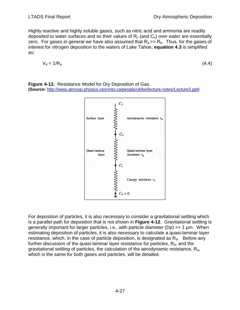
Estimation of Vd requires consideration of the controlling processes that comprise it. Vd is commonly estimated using a model of resistances or conductances analogous to electrical circuitry. For gases, the total resistance to transfer (Rtotal) is the sum of three basic resistances acting in series (see Figure 4-12 ). These are the aerodynamic resistance (Ra), the “quasi-laminar” boundary layer (or viscous sub-layer) resistance (Rb), and the surface (or vegetation canopy) resistance (Rc). Ra is the resistance to mixing through the boundary layer toward the surface by means of the dominant process, turbulent transport. A large value of Ra would indicate a relative lack of turbulence. The quasi-laminar layer resistance, Rb, is resistance to movement across the thin layer (0.1 – 1 mm) of air that is in direct contact with a surface and not moving with the mean flow of the wind. Through this thin layer, in the absence of turbulence, the primary transport process for gases is molecular diffusion. For gases the quasi-laminar layer resistance is designated as Rb. For particles the important transport processes in this layer are Brownian motion and inertial impaction). To differentiate from gases, the quasi-laminar layer resistance for particles is designated as Rd. Rc, the resistance of a compound to uptake by a surface, varies both with the surface and the chemical species or physical state (gas or particle). For gases the deposition velocity can be expressed as:
Vd = 1/(Ra + Rb + Rc) (4.3)
LTADS Final Report Dry Atmospheric Deposition
4-27
Highly reactive and highly soluble gases, such as nitric acid and ammonia are readily deposited to water surfaces and so their values of Rc (and Co) over water are essentially zero. For gases in general we have also assumed that Ra >> Rb. Thus, for the gases of interest for nitrogen deposition to the waters of Lake Tahoe, equation 4.3 is simplified as:
Vd = 1/Ra (4.4)
Figure 4-12. Resistance Model for Dry Deposition of Gas. (Source: http://www.atmosp.physics.utoronto.ca/people/ulrike/lecture-notes/Lecture3.ppt)
For deposition of particles, it is also necessary to consider a gravitational settling which is a parallel path for deposition that is not shown in Figure 4-12 . Gravitational settling is generally important for larger particles, i.e., with particle diameter (Dp) >> 1 µm. When estimating deposition of particles, it is also necessary to calculate a quasi-laminar layer resistance, which, in the case of particle deposition, is designated as Rd. Before any further discussion of the quasi-laminar layer resistance for particles, Rd, and the gravitational settling of particles, the calculation of the aerodynamic resistance, Ra, which is the same for both gases and particles, will be detailed.

LTADS Final Report Dry Atmospheric Deposition
4-28
4.3.1.1 Primary Calculation of Aerodynamic Resistance The aerodynamic resistance, Ra, is controlled by the level of atmospheric turbulence available to transport gases and particles in the air into close proximity to the surface. The subsections that follow describe methods for calculation, including for completeness, one that was not applied in these calculations. All require estimation of the Monin-Obhukov Length (L) scale, which is a stability parameter. Also discussed, in the final subsection, are caveats regarding estimation of Ra for the near shore zone during offshore flow. Common assumptions about the variation in wind speed with height through the surface layer may not hold at the measurement heights due to larger values of the aerodynamic roughness length (Z0) over land. A commonly used formulation for aerodynamic resistance assumes similarity between turbulent transport of chemical species and turbulent transport of momentum. That formulation is: Ra = U / (U*)
2, (4.5) where U is the wind speed and U* (pronounced Ustar) is the friction velocity. The friction velocity is a measure of the shearing stress of the wind on the surface below. It is defined as the square root of the surface shear stress divided by the density of air. Methods used to estimate U* are provided in the following sections. The wind speed is usually directly measured. Although friction velocity may be determined by direct measurement of momentum flux by the eddy covariance (EC) method, friction velocity is less exactly but commonly estimated from more routine meteorological measurements of wind speed and temperature at multiple heights. LTADS calculated the friction velocity and aerodynamic resistance using the formulation of Byun and Dennis (1995) adapted for use over water. The relationship of wind speed (Uz) to height above the surface (z) is the logarithmic profile adjusted for stability of the atmosphere as described by the Monin Obhukov Length scale (L). Their formulation depends on whether the atmosphere is stable or unstable, as indicated by the sign of L. For the stable atmosphere case, where L > 0 (based on Tair > Twater),
Uz = [(U*)/(k)] * [ln((z)/ Z0) + 4.7 * (z - Z0/L)], (4.6) where:
k = Von Karmen constant = 0.4 Z0 = aerodynamic roughness length U* = friction velocity. The square of the friction velocity equals the wind-induced shear stress at the surface divided by density of air.
For the unstable atmosphere case, where L < 0 (based on Tair < Twater), Uz = [(U*)/(k)] * [ln(numerator/denominator)], (4.7)
where: numerator = [(1 + 16 * z / |L|) – 1] ½ * [(1 + 16 * Z0 / |L|) + 1] ½ denominator = [(1 + 16 * z / |L|) + 1] ½ * [(1 + 16 * Z0 / |L|) - 1] ½

LTADS Final Report Dry Atmospheric Deposition
4-29
Thus, with thermally neutral atmospheric conditions, the wind speed is logarithmic with height and the terms that involve the Monin-Obhukov Length scale (L) modify the wind profile in response to the influences of non-neutral thermal stratification. A physical meaning for the Monin-Obhukov Length scale (L) is that it is proportional to the height in the surface layer at which the shear forces are first dominated by the buoyant forces. Shear forces generally produce turbulent kinetic energy (TKE) near the surface whereas buoyancy forces generally increase with height through the surface layer and commonly produce TKE due to convection or suppress TKE under stable conditions. Under convective conditions buoyant and shear production of TKE are approximately equal at a height of z = -0.5 L. The Monin-Obhukov length scale is defined in terms of the vertical fluxes of momentum and heat evaluated near the surface and is derived from a non-dimensional form of the turbulent kinetic energy equation. Appendix F and Stull (1988) among others discuss how L represents the relative importance of sources of TKE based on terms in the TKE equation. LTADS did not directly measure fluxes of momentum and heat flux; thus, to determine hourly values of L, a simple parameterization provided by Hanna et al. (1985) and used in the CALMET meteorological model (Scire et al., 2000a) for calculation of momentum flux over water, was employed.
L = (Ta + 273.16) [((0.75 + (0.067)(U10))/1000]3/2 / [(E2)(Ta – Tw)] (4.8) where:
Ta is the observed air temperature U10 is the wind speed extrapolated to 10 meters Tw is the observed water temperature E2 = 0.0051
Because the observed water temperature may be sensitive to the wind speed during that hour and to the depth of the observation, the sensitivity of the deposition estimates to an arbitrary bias in water temperature was investigated. With an arbitrary bias of 3 ºC (5.4 ºF) added to the observed water temperature for all hours, estimated annual dry deposition increased by about 7 to 16 percent. The increases varied between the pairs of air quality and meteorological monitoring sites used and differences in the estimates were generally largest for gases and fine particles. The sign of any actual bias in observed water temperature due to the effects of wind speed or measurement depth would depend largely on the sign of the net radiation at the water surface. Thus, the effects would tend to average out over diurnal cycles and across seasons and the net effect of bias in observed water temperatures should have minimal effect on the annual deposition estimates.
The formulation of aerodynamic roughness length (Z0) over water is from Hosker, (1974) and takes the following form. Z0 = (0.000002)(U10)
5/2 (4.9)

LTADS Final Report Dry Atmospheric Deposition
4-30
As discussed in Section 4.3.1.5, near the shoreline the value of Z0 also depends strongly upon wind direction and this was taken into account in the iterative solution. In the absence of resource intensive direct measurements of the friction velocity (U*), the value of U* can be calculated from the wind speeds and temperatures observed at two or more heights. By using an iterative method it is also possible, based on water temperature and meteorological observations at a single height, to calculate the values of friction velocity (U*), aerodynamic roughness length (Z0), and Monin-Obhukov Length scale (L). Multiple iterations are needed because of the interdependence of these variables. LTADS used an iterative solution in which Z0 and L were estimated using formulations that require input of an estimated wind speed at 10 meters (U10). For initial estimates of Z0 and L the wind speed at the instrument height was substituted for wind speed U10 in equations 4.8 and 4.9 . Successive estimates of U10 were made with equations 4.6 and 4.7 and Z0 and L were recalculated upon each new estimate of U10. Note that the equations 4.8 and 4.9 are specific to applications over water. From equations 4.5 and 4.6-4.7 the aerodynamic resistance, Ra, takes the following forms. For the stable atmosphere case, where L > 0 (based on Tair > Twater),
Ra = [1/(k * (U*))] * [ln(z/ Z0) + 4.7 * (z/L)], (4.10) For the unstable atmosphere case, L < 0 (based on Tair < Twater), Ra = [1/(k * (U*))] * [ln(numerator/denominator)], (4.11)
where: numerator = [(1 + 16 * z / |L|) – 1] ½ * [(1 + 16 * Z0 / |L|) + 1] ½ denominator = [(1 + 16 * z / |L|) + 1] ½ * [(1 + 16 * Z0 / |L|) - 1] ½
4.3.1.2 Aerodynamic Resistance from Bulk Estimate of Momentum Flux For comparison purposes, LTADS also estimated the aerodynamic resistance by applying a bulk coefficient method to calculate momentum flux and friction velocity and using the results in equation 4.5 . The CALMET model (Scire, et al., 2000) uses the same bulk coefficient method for calculating momentum flux over water. The friction velocity, U*, was calculated in m/s as by Garratt, et al. (1977):
U* = U10 (CUN) ½, (4.12)
where the bulk coefficient, CUN is given by:
CUN = (0.75 + 0.67 * U10 ) / 1000, (4.13) Ra is then calculated from equation 4.5 in units of s/m or in units of s/cm as
Ra = [(U10 ) / (U*)2 ] /100, (4.14)

LTADS Final Report Dry Atmospheric Deposition
4-31
The simple formulations for the aerodynamic resistance and the friction velocity provided by equations 4.12 – 4.14 do not address the effects of thermal stability or convection and, thus, the estimates they provide only reflect the effects of wind speed. Estimates of 1/ Ra, provided by the formulation of Byun and Dennis (described in the previous section), were compared the estimates provided by the bulk coefficient calculation. The comparison was restricted to estimates for the open water areas (more than 1 km offshore) because the bulk coefficient method in the form shown in equations 4.13 and 4.14 is only applicable to open water areas. The estimates from the formulation of Byun and Dennis averaged about one third higher with some variation due to differences in the wind speeds and stability between sites and seasons. Recall from equation 4.4 that for the gases of interest, the deposition velocity is predicted as 1/ Ra. The values for 1/Ra provided by the bulk coefficient method were merely used as a gross check on the estimates provided by the formulation of Byun and Dennis. They were not otherwise utilized in the estimates of annual deposition which are presented later in this chapter. Those estimates of dry deposition are based on the formulation of Byun and Dennis. In previously reported comparisons (ARB, January 2005), due to time constraints, the observed wind speeds were used directly in equations 4.13 and 4.14 without having been extrapolated to 10 meters. Since then, staff compared the results of the bulk calculation of aerodynamic resistance (equation 4.14 ) using the wind speed at the measurement height and also at the reference height of 10 meters and found that the change in results was minimal.
4.3.1.3 Potential Alternative Calculation of Aerodynamic Resistance Valigura (1995) modeled deposition of HNO3, making the common assumption that Ra >> Rb. He assumed similarity between turbulent transport of heat and chemical species for calculation of Ra. Heat flux was modeled by iterative solution of a surface energy balance. To verify the model, Valigura compared measured and modeled values of skin temperature and heat flux. The results were reported to be inconclusive and differences, between measured and modeled values, were attributed to a possible mismatch in scales of observations obtained with aircraft-based and boat-based instruments.
For completeness and comparison with the current results, it may be possible to make calculations by an adaptation of Valigura’s method. That would require information on the balance of net radiation based upon measurements or parameterizations suitable for the altitude of Lake Tahoe and availability of supporting meteorological data (e.g., cloud type and height). However, adequate data for verification of the modeling may not be available and this investigation could not be attempted within the timeframe available for releasing this final report. However, if this type of analysis were attempted in the future, observations of water skin temperature and incoming short- and long-wave radiation would be very useful for verification.

LTADS Final Report Dry Atmospheric Deposition
4-32
4.3.1.4 Potential for Independent Validation of Aerodynamic Resistance Estimates Because the aerodynamic resistance is defined by fluxes of heat and momentum, there is a potential for independent validation of estimates of aerodynamic resistance by comparing modeled fluxes with observed fluxes. Although not collected as part of LTADS, some eddy covariance measurements of momentum flux, heat flux, sensible heat flux, and friction velocity are available from experiments at Lake Tahoe and elsewhere. Use of these data would require quality assurance analyses first, but they could be used for an independent estimate of the uncertainty in the values of aerodynamic resistance that are predicted using the methods discussed above.
4.3.1.5 Caveats Regarding Roughness Length and Aerodynamic Resistance The formulations used here to estimate Ra assume a logarithmic wind profile (modified for the effects of stability). But the assumed form of the wind profile is not valid at heights of less than 50 times the aerodynamic roughness length (Brutsaert, W., 1982). The following paragraphs define the aerodynamic roughness length and describe its treatment in the calculations of aerodynamic resistance, particularly for situations with measurement heights or reference heights less than 50 times Z0.
The aerodynamic roughness length scale, Z0, represents the effects of surface roughness on the wind flow as that roughness affects the generation of shear induced turbulence. The aerodynamic roughness length is not equal to the height of individual roughness elements, but there is a one-to-one correspondence between these roughness elements and the aerodynamic roughness length. The amount of downwind turbulence generated by wind flow over a rough surface is a factor in determining the vertical profile of wind speed and the aerodynamic resistance, Ra. Z0 is used to represent this effect in the equations of the vertical profile of wind speed, momentum flux, and aerodynamic resistance. Particularly for larger values of Z0, the aerodynamic resistance and the deposition velocity are sensitive to Z0. (The zero plane displacement height, defined as the height at which the horizontal wind speed goes to zero, has been ignored in these calculations, but does not significantly affect the calculations.) Over open water, the shear force of the wind causes waves to develop and Z0 is commonly estimated as a function of either friction velocity or wind speed. Various formulations are available dating from the classical formulation by Charnock (1955) to the formulation used here (Hosker, 1974) that was presented as equation 4.9. This calculation of Z0 also applies near shore when the wind direction is onshore (from Lake toward land). When the wind direction is offshore (from land to water), there is advection of greater turbulence associated with greater surface roughness elements over land as was observed by Sun (2001) in coastal environments. The effect is to decrease aerodynamic resistance and increase deposition velocity in the near-shore zone when the wind is offshore. This effect is implemented by making separate calculations for offshore wind direction and onshore wind direction. During offshore flow, to represent

LTADS Final Report Dry Atmospheric Deposition
4-33
conditions at the shoreline (and at the piers where the meteorological measurements were made) the aerodynamic resistance is calculated using an aerodynamic roughness length of 1 meter to characterize the effects of the land area immediately upwind. This value of Z0, for offshore wind direction, in turn affects the calculation of the friction velocity and extrapolation of the wind speed to 10-meters above the surface. The result is to decrease Ra and increase deposition velocity. The advection of turbulence from over land is assumed to affect the aerodynamic resistance from the shoreline to a distance of 1 km offshore. The computations assume a linear decay of the near-shore Ra to the open-water Ra at a distance of 1 km offshore. Over open water and in the near-shore zone with onshore flow, the Z0 is sufficiently small, on the order of 0.0001 m, that the assumed form of the wind profile is reasonable at heights well below the heights of wind observations. However, with offshore winds, the larger surface roughness elements over land affect the flow over the near-shore waters increasing the aerodynamic roughness length to 1 or 2 meters, so that the assumption of a log wind profile is not satisfied near the surface. Even with a moderate assumption of Z0 = 1 m in the vicinity of the pier mounted meteorological instruments, the assumed form of a basically logarithmic wind profile is thus not theoretically valid at the measurement heights which are less than 10 meters. This constraint is widely ignored in the literature, largely because little error is introduced for most uses of the logarithmic profile. But this turns out not to be the case for the calculation of the aerodynamic resistance. The calculated values of Ra are inordinately sensitive to Z0 when Z0 is of the same order of magnitude as the observation height Z. For this situation the calculated values of Ra were unreasonably small and the resulting estimates of deposition velocity were unrealistically large. This was remedied by setting a lower limit of 1/6 s/cm for Ra for the “best” estimate of deposition rates which results in and upper limit of 6 cm/s for deposition velocity of gases. For the lower and upper limit estimates the limitations on 1/Ra were set at 3 and 10 cm/s respectively. Selection of these values were based on literature indicating the maximum observed deposition rates over water for a reactive soluble gas (SO2) were in the range of 3 to 4.5 cm/s and a desire, consistent with the LTADS purpose, to ensure that for the upper-limit estimate the deposition velocities and deposition rates would be sufficiently inclusive. Sehmel (1980), citing Whelpdale and Shaw (1974) and others, reports observed deposition velocities for SO2 to water surface ranging from 0.16 to 4 cm/s, with the range of values dependent on atmospheric stability. In the near-shore zone at Lake Tahoe offshore flow frequently consists of down-slope cold air drainage over a warmer water surface. Thus, near shore during nocturnal and early morning offshore flow periods in most seasons, thermal instability is the norm. Thus, buoyant forces are expected to generate turbulence in addition to any shear induced turbulence. However, with typically low wind speeds production of turbulence due to wind shear should be weak. Thus, the assumptions for aerodynamic resistance in the near-shore zone during offshore flow periods are expected to provide conservatively large deposition velocities. The lower limit of 1/6 s/cm for Ra and resulting upper limit deposition velocity of 6 cm/s for gases was invoked in the near-shore areas for most hours of offshore flow but was not invoked for mid-Lake areas or

LTADS Final Report Dry Atmospheric Deposition
4-34
near-shore areas during onshore flow. Thus, this limit is only applied in the near-shore region when larger values of Z0 were used during hours of offshore flow. The near-shore region affected by the upper limit on deposition velocity was estimated to extend 1 km from shore and to comprise 20 percent of the surface area of the Lake.
4.3.1.6 Quasi-laminar Layer Resistances (Rb) for Gases and (Rd) for particles Resistances Rb for gases and Rd for particles are their resistances to transport through the very thin (0.1 – 1 mm) viscous sub-layer at the surface. This layer is also referred to as the quasi-laminar layer (Hicks, 1982) or the laminar deposition layer (Scire et al., 2000a). Others have used the term viscous layer. The quasi-laminar resistance (Rb) for gases is differentiated from the quasi-laminar resistance for particles (Rd). Use of the term “quasi” can serve as a reminder that for rough surfaces a laminar layer may only be intermittently present and that the formulations for smooth surfaces and rough surfaces differ. Transport through this thin layer is by molecular diffusion for gases and by Brownian motion and impaction for particles. For gases, Rb is generally considered to be very small compared to Ra. However for estimating the deposition velocity of particles, Rd must be explicitly calculated. Because the quasi-laminar layer resistance for particles (Rd) and the particle gravitational settling velocity (Vg) require some of the same variables, the formulas for their calculation are grouped in Section 4.3.2.
4.3.1.7 Surface Resistance (Rc) The surface resistance of water is very small (effectively 0) for both particles and highly reactive or soluble gases such as nitric acid or ammonia. The relative contribution of nitrogen to the Lake by deposition of other non-soluble, non-reactive gaseous N species, such as NO2, is very small because Rc is a large limiting resistance and the deposition velocity is very small. Although LTADS is not estimating deposition over land surfaces, it may be of interest that for moderately reactive chemical species, such as ozone or NO2, the surface resistance, Rc, over land varies spatially with differences in land use and vegetation type and temporally with biophysical responses of vegetation to light, moisture, etc.
4.3.2 Deposition of Particles The equations for deposition of particles are similar in form to the equation for deposition of gases but differ in several particulars. For estimating deposition velocities for particles, gravitational settling velocity, Vg, must be considered in addition to the resistances discussed above and shown in Figure 4-12 for gases. Note that gravitational settling is an alternative and competing pathway. However, it is primarily important for deposition of larger (> 10 µm) particles. Although the quasi-laminar layer resistance for particles is analogous to that for gases, its formulation must differ to represent the different processes (Brownian motion and impaction) acting to transport particles (rather than gas molecules) across that layer. The primary mechanism is Brownian motion for fine particles, and impaction for larger particles (of Dp >>1 µm). The quasi-laminar layer resistance for particles, Rd, is greatest for particles in the size

LTADS Final Report Dry Atmospheric Deposition
4-35
range of Dp ~0.3-0.5 µm because the rates of Brownian diffusion and impaction for these particle sizes are both low. For this size range, Rd over water can be a primary constraint to deposition causing a minimum in Vd for accumulation mode particles. A representation of the effects of particle size on deposition velocity is shown in Figure 4-13.
4.3.2.1 Traditional Formulation of Particle Deposition Velocity In equations 4.1 - 4.4 and Figure 4-12 , we presented the general model for deposition of gases. The equations for deposition of particles are similar in form but add the effects of settling velocity of large particles as a competing pathway taking the form of either the commonly used equation 4.15 or the corrected equation 4.18 . The formulation of particle deposition given in equation 4.15 is common to many current air quality models (e.g., CALPUFF and ISCST3) was initially used by LTADS. Many authors, e.g., Slinn and Slinn (1980), Pleim et al. (1984), and Seinfeld and Pandis (1998) have presented this general form shown below.
Vd = Vg + [1/(Ra + Rd + Ra * Rd *Vg)] (4.15)
The gravitational settling velocity, Vg, is not simply additive because it is a parallel path in competition with the path shown in Figure 4-12 . The equations for the gravitational settling velocity, Vg, and quasi-laminar layer resistance, Rd, are given below along with additional variables used in their calculation. Note that the formulation for the aerodynamic resistance, Ra, is that of Byun and Dennis, which was presented previously and is applicable to either particles or gases.

LTADS Final Report Dry Atmospheric Deposition
4-36
Figure 4-13. Deposition Velocity is a Non-Linear Function of Particle Size. Source: http://www.atmosp.physics.utoronto.ca/people/ulrike/lecture-notes/Lecture3.ppt
Resistance is the inverse of conductance and is a means to quantify limitations of a particular conductance mode. Movement of particles across the quasi-laminar layer is by Brownian motion and inertial impaction. Thus, the quasi-laminar layer resistance describes to what extent transfer of particles across the layer by Brownian motion and inertial impaction limits the rate of deposition. The quasi-laminar resistance for particles (Rd) is analogous to but differentiated from the quasi-laminar layer resistance for gases (Rb) which expresses the extent to which conductance of gas molecules across the quasi-laminar layer by molecular diffusion is a rate limiting step for deposition of gases. Rd = (1/( U*)) / (Sc)-2/3 + 10-3/St, (4.16)
where: Sc = Schmidt number = Va / Db, where:
Va = viscosity of air = 0.15 cm2/s Db = Brownian diffusivity (cm/s) = 8.09 * (Ta + 273.16) * 10-10 * Scf/diam_pm, where: Scf = Cunningham slip correction factor
= 1 + (2 * (x2) * (a1 + a2 * exp(-a3 * diam_pm/x2)) / (diam_pm * 0.0001),
where: x2 = 0.0000065

LTADS Final Report Dry Atmospheric Deposition
4-37
a1 = 1.257 a2 = 0.4 a3 = 0.000055 diam_pm = measured, or assumed, diameter of particle
St = Stokes number = (Vg/ag) * (U*)2 / Va, where:
ag = acceleration due to gravity (981 cm/s2) The formulation presented here for quasi-laminar boundary layer resistance is strictly speaking only applicable to aerodynamically smooth surfaces, although this distinction is frequently ignored in the literature. However, the distinction between smooth and rough formulations is not critical to the LTADS estimates of deposition. The differences in resistance are significant only for fine particles which make up a minor fraction of the deposited particle mass. Also, for most hours over Lake Tahoe, the wind speeds are sufficiently low that the water surface is aerodynamically smooth. The frequency distribution of wind speeds presented in Table 4-2 and discussed in Section 4.2.1 suggests that the lake surface is aerodynamically rough for only a few percent of the hours, in transition from smooth to rough for about one-fourth of the hours, and aerodynamically smooth for over two-thirds of the hours. The gravitational settling velocity, Vg, was introduced previously. It is primarily dependent of particle size and density. In units of (cm/s) it is calculated as:
Vg = [(ρp - ρa) * ag * [diam_pm]2 c2] * Scf / (18* Va), (4.17) where:
ρp = density of particle; value input (~1-3 g/cm3) ρa = density of air (g/cm3)
= 0.012 *[(Ta + 273.16)/273.16] * (Pa / 1000), where: Pa = atmospheric pressure (mb)
c2 = 0.00000001 cm2/mm2
4.3.2.2 Corrected Formulation of Particle Deposition Velocity Although equation 4.15 is still very widely applied, Venkatram and Pleim (1999) showed that it violates the fundamental physical constraint of mass conservation and derived a corrected formulation that satisfies that constraint.
Vd = Vg/[1-e-Vg(Ra +Rd +Rc)] (4.18)
Substitution of equation 4.18 for equation 4.15 brings a small reduction in estimated deposition velocities. The reductions in annual deposition velocity vary mainly with particle size and also vary slightly with the seasonal and site specific meteorological conditions. Annual deposition velocities for fine (<2.5 µm) and large (>10 µm) particles were only reduced by about 1 to 6 percent. Predicted deposition velocities for coarse particles (2.5 < dp < 10 µm) generally decreased by between 10 and 15 percent with

LTADS Final Report Dry Atmospheric Deposition
4-38
use of equation 4.13 . The percent reduction in estimated deposition velocity as a function of particle size is shown in Figure 4-14 . In contrast to previous reports and memos, the deposition rates for particles reported here are based upon equation 4.18 . By use of the corrected formula (equation 4.18 in place of 4.15) estimates of deposition velocity for coarse particles are reduced by about 10 to 15 percent, and estimates of the deposition of fine and large particles are reduced by less than 10 percent. This caused a modest reduction in estimates of deposition amounts of phosphorus and particles. However, there was little effect on the estimates of nitrogen deposition because the deposition of aerosol nitrogen (nitrate and ammonium) is dwarfed by deposition of gaseous ammonia and nitric acid.
Figure 4-14. Percent change in annual average deposition velocity by particle size for mid-Lake areas in response to substitution of equation 4.18 (Venkatram and Pleim, 1999) for equation 4.15 (Pliem, et al., 1984; Seinfeld and Pandis, 1998).
Changes in calculated deposition velocity varied slightly due to differences in meteorological conditions at U.S. Coast Guard Pier, TDR1 buoy, and Tahoe Vista pier.
4.3.2.3 Effects of Hygroscopic Particle Growth The potential effects of growth of particle size by uptake of water vapor are not quantified in the deposition rates presented here. The deposition of particles in general, and phosphorus-containing particles in particular, could be increased somewhat by hygroscopic growth but that effect is not expected to be large. First, the particles that
Percent Change of Deposition Velocity (Midlake)vs. Particle Diameter
-18%
-16%
-14%
-12%
-10%
-8%
-6%
-4%
-2%
0%0 10 20 30 40 50 60 70
Particle Diameter (microns)
Cha
nge
(New
-Old
)
USCG_LF
TDR1_SW
TV_TB

LTADS Final Report Dry Atmospheric Deposition
4-39
contain phosphorus are not necessarily hygroscopic. Second, the amount of growth before deposition occurs may be minimal. Early modeling of particle growth (Williams, 1982) assumed equilibrium between water vapor and aerosols. However, Zufall et al. (1998) concluded that particles larger than 0.1 µm do not reach equilibrium before depositing and showed that models assuming equilibrium can overestimate the effects of hygroscopic growth on deposition by as much as a factor of 5. Hygroscopic particle growth may affect deposition rates positively or negatively in amounts that depend on the environmental conditions and the chemical composition and initial size of the particles. Using alternative models that do not assume equilibrium, Pryor, et al. (2000) indicated hygroscopic growth may increase the deposition rate significantly for highly hygroscopic particles in the size range of Dp ~ 0.3-10 µm, but the particles observed in LTADS are primarily comprised of less hygroscopic constituents.. The size of NH4NO3 aerosol is likely Dp ~ 0.3-6 µm but NH4NO3 is only expected to contribute a very minor amount of the N load compared to gaseous HNO3 and NH3. For Dp < 0.3 µm and moderate wind speeds (U<10 m/s), particle growth is expected to decrease Brownian diffusion, thus increasing Rd and thereby decreasing Vd. For Dp > 10 µm the effect of hygroscopic growth is to increase impaction and Vg but the relative change in deposition velocity is less. At higher wind speeds, the viscous layer is thinner and inertial impaction acts more effectively so that particles deposit more quickly and the effects of particle growth are minimal.
4.3.2.4 Effects of Spray The estimated annual deposition rates presented in this report are based upon hourly concentrations and deposition velocities calculated without explicit consideration of the effects of spray. The discussion which follows illustrates that the effects of spray on the annual deposition rates at Tahoe must be minor. The main points that are pertinent and developed below are: 1) dry deposition over water is enhanced for specific particle sizes when strong winds generate breaking waves and spray, 2) wind speeds sufficient to substantially affect deposition rates through the generation of breaking waves and spray occur less than six percent of hours on an annual basis at Lake Tahoe, 3) a substantial portion of modeled increases in deposition velocity were associated with hygroscopic growth, 4) the presence of spray did not appreciably increase the modeled deposition velocity of particles larger than 3 or 4 microns, and 5) during high winds atmospheric concentrations will generally be at a minimum, due to enhanced mixing and dilution. Pryor and Barthelmie (2000) indicate that wind blown spray associated with breaking waves and bubble bursting have the potential to increase particle deposition by three processes. Firstly, ejection and deposition of droplets may induce turbulence in the laminar surface layer. Secondly, as they fall, droplets may sweep in-situ gases and particles towards the surface. Finally, as particles are transported through the near-surface layer they will encounter higher humidity levels when spray is present and if the particles are hygroscopic they will absorb water and grow in size (affecting their diffusivity). Pryor and Bartholemie explicitly modeled these three processes and their predicted effects on deposition velocities for hygroscopic particles (NO4NO3) of various sizes and with various wind speeds.

LTADS Final Report Dry Atmospheric Deposition
4-40
They reported that with wind speeds of 5 m/s bubble bursting and spray increased modeled deposition rates by up to ten percent for small (< 3 or 4 µm) particles but deposition rates of larger (> 4 µm) particles were not appreciably affected by spray. They report that these modeling results were consistent with results of wind tunnel studies of deposition over water (Larsen et al., 1995) which showed that increasing simulated area of white cap cover from 0 to 25 percent increased average deposition velocities by less than 30 percent. With higher (10 and 15 m/s) wind speeds, the deposition velocities modeled by Pryor and Barthelmie for small (< 4 µm) hygroscopic particles increased by factors of 1.5 and 2 respectively but did not appreciably increase deposition rates for larger (> 4 µm) particles. Although deposition velocities for particles smaller than 4 µm could be significantly increased (e.g., by a factor of two) during hours with such high winds this is only a very small fraction of the total hours and about one half or less of the total particle mass. Frequency distributions of wind speed and direction were reported in Tables 4-2 and 4-3 as meteorological context for understanding patterns of deposition at Lake Tahoe. Note that wind speeds of 7-10 (and > 10 m/s) were only observed during 4 (and 2) percent of hours at the windiest site, buoy TDR2. Thus, the effect of spray on annual deposition rates is probably less than 2 percent even if there were no correlation between wind speed and concentrations. However, we know that higher wind speeds will generally result in significantly increased mixing and substantially lower concentrations compared to the annual average. Thus, although the effect of spray on deposition rates for small particles during specific hours can be significant, the effects of spray are expected to increase estimated annual deposition rates at Lake Tahoe by less than one percent. Thus, mechanistic modeling or explicit calculations of the effects of spray on deposition rates for individual hours would be an inappropriate use of resources within the goals and framework of LTADS.
4.4 Short- term Targeted Studies of PM Distribution The discussion in section 4.3 explains how particle size influences deposition. Because the LTADS baseline monitoring was limited in spatial resolution and was limited to three gross size ranges (<2. 5 µm, 2.5-10 µm, >10 µm), additional information on size distributions and their spatial variations is desirable to confirm that deposition calculations based on the simplified LTADS size data would reasonably represent the deposition environment at Lake Tahoe. This section describes the salient findings of a series of experiments conducted during LTADS using optical particle counters to characterize the temporal and spatial variation of particle size distributions.
4.4.1 Overview of Particle Count Experiments The overall goal was to understand how concentrations and particle size distributions might differ with location and time (compared to measurements at the LTADS sites) and to better understand how those gradients might affect the deposition estimates.
4.4.1.1 Program Goals The particle count experiments addressed these areas of concern:

LTADS Final Report Dry Atmospheric Deposition
4-41
• Spatial variation among monitoring environments (e.g. urban vs. rural). • Spatial variation between lakeshore and mid-lake areas • Spatial variation near roadways and monitoring sites due to dilution and
deposition of roadway emissions • Temporal variation due to shifts in wind direction.
Due to limitations of time and funding, these experiments were largely exploratory, with only enough data collected in each experiment to permit evaluation of general structure and trends. The data presented here are strongest when viewed qualitatively, showing how particle concentrations and size distributions vary at Lake Tahoe. Although the sampling periods were chosen to represent conditions "typical" of the Tahoe basin, the actual particle concentrations measured in these experiments may not be representative of long term conditions. The particle size count "bins" (0.5-1, 1 - 2.5, 2.5 – 5, 5 - 10, 10 - 25, and 25+ µm) span the ranges of interest for lake clarity, from the particles that scatter light in the lake (0.5 - 2.5 µm) to large soil particles which can deliver significant amounts of mineral nutrients and support algal growth. Particles less than 0.5 µm were not counted, but these particles do not effectively scatter light and do not contribute significant mass. The LTADS filter-based measurements do include the fraction of combustion-derived and secondary particles smaller than 0.5 µm; since the deposition calculations are based on the filter data, their absence in the count data is not carried over to the deposition estimates.
4.4.1.2 Particle Counter Calibration and Validation of Data The principal instrumentation used in the dust experiments was a set of Climet CI-500 optical particle counters. These counters draw a stream of air through an optical chamber where, one-at-a-time, particles in the air stream pass through the beam of a solid-state laser. Light scattered by a particle is sensed photoelectrically, with the strength of the scattering converted into particle size based on scattering cross-section, and the number of particles in each size "bin" is recorded over a standard sampling period (for LTADS, typically one or twenty minutes). There is a maximum count rate, beyond which multiple particles are sensed together (causing mis-sizing), but concentrations observed in the Tahoe region never exceeded the count-rate capability of the instruments. These instruments are calibrated at the factory, and cannot be adjusted by the user. Validation of calibration was determined by side-by-side testing of multiple instruments before and after each field experiment. An example is shown as Figure 4-15 . Repeated intercomparisons showed minimal drift over the life of the LTADS field program. After each experiment, counts from instruments showing statistically significant bias in any size bin relative to CI-500 #105 were adjusted to eliminate that bias in final particle counter data.

LTADS Final Report Dry Atmospheric Deposition
4-42
The relationship between counts and mass was investigated by comparing count-estimated hourly aerosol mass with hourly BAM data for a week at the SOLA monitoring site (Figure 4-16 ). Aerosol volume was estimated by assuming that all particles in each size bin were spheres with a diameter equal to the geometric mean of the maximum and minimum size for the bin. Volume was converted to mass by assuming a particle density of 1 for all particles less than 2.5 µm, 2.5 for all particles over 10 µm, and intermediate values for particles between these two ranges (Table 4-4 ). These densities imply an increasing geological contribution for larger particle size, with the density of quartz (2.5) representing geological materials. Fine organic particles from combustion are assumed to be dominated by organics with a density near 1 and nitrates and sulfates are assumed to have a similar density due to their association with water. Although the BAM derived mass values were not expected to be reliable for individual hours the time series of mass from the two methods are similar and the scatter plot shows an r2 of 0.4. Thus it appears that the particle counts can provide a useful semi-quantitative indication of particle mass. The count-based mass estimates do not include any particles smaller than .5 µm but this mass is not significant.

LTADS Final Report Dry Atmospheric Deposition
4-43
Figure 4-15. Comparison of data from between two collocated CI-500 samplers.
Table 4-4. Assumed densities of particles by size bin. These densities were utilized to generate count-based estimates of mass, for comparison with BAM TSP observations of mass (see Figure 4-16).
Particle Size (µm) Assumed Density (g/cc) 0.5 - 1 11 - 2.5 12.5 - 5 1.55 - 10 2
10 - 25 2.5> 25 2.5
101 102 103 104 105 1062 34 2 34 2 34 2 34 2 34
CI-500 #105
101
102
103
104
105
106
235
235
235
235
235
CI-
500
#106
0.5 - 1.0 um1.0 - 2.5 um2.5 - 5 um5 - 10 um10 - 25 um

LTADS Final Report Dry Atmospheric Deposition
4-44
Figure 4-16. Comparison of Size-Resolved CI-500 (#105) Interpreted Aerosol Mass with Hourly TSP BAM Data at SOLA.
4.4.2 Spatial Variation among Terrestrial Monitorin g Environments Since land use in the LTADS study area ranges from urban to wilderness, comparisons were run among three sites - the urban SOLA site, the upland BLIS IMPROVE site, and a remote, unpopulated site at about the same elevation but outside the Tahoe Basin (Burnside Lake in the Hope Valley region, 24 km south of SOLA).
4.4.2.1 Remote Rural Sites The Hope Valley area has minimal population, and Burnside Lake site is about 6 km from the nearest settlement or paved road. The nearest particle source was a small campground about 0.25 km from the measurement site. The rural sample within the Tahoe Basin was taken at the BLIS IMPROVE site, an unpopulated area on the west side of the basin about 200 m above the lake. The particle size distributions obtained were taken the morning after a rain event and are generally representative of "clean" conditions in the region (Figure 4-17 ). The vertical scale dM/dD is the change in particle mass per change in particle diameter, thus it is a measure of relative mass within size fractions.
0
10
20
30
40
50
60
TS
P (
µg/m
3 )
9/4/
2003
12:
00:0
0 AM
9/5/
2003
12:
00:0
0 AM
9/6/
2003
12:
00:0
0 AM
9/7/
2003
12:
00:0
0 AM
9/8/
2003
12:
00:0
0 AM
9/9/
2003
12:
00:0
0 AM
START HOUR
1-HR PARTICLE COUNT TSP 1-HR BAM TSP
0 10 20 30 40 50
PARTICLE COUNT TSP (µg/m3)
0
10
20
30
40
50
60
BA
M T
SP
(µg
/m3 )
TSPBAM = (.99±.04) TSPCOUNT; R2 = .41

LTADS Final Report Dry Atmospheric Deposition
4-45
Figure 4-17. Particle size distributions at remote rural sites in Hope Valley (Burnside Lake) and Tahoe Basin (BLIS) on morning of June 26, 2003.
Vertical bars are 1-σ range for each size bin. Steps in cumulative mass plots denote widths of size bins.
The mean (±1σ) TSP (Total Suspended Particulate) concentration at Burnside Lake was 23±12 µg/m3 (the large variability suggests possible influence by our vehicle travel to the site); TSP at BLIS for the same period was 16±3 µg/m3. The cumulative mass curves show that both sites were dominated by larger particles; fines (<2.5 µm) were less than 5 percent of the estimated mass, while large particles (>10 µm) were nearly 2/3 of the total. Given the wide variability (denoted by the vertical bars) and the overall low aerosol loading, these sites can be considered comparable. The shapes of these particle size distributions show the multi-modal nature of particles. The larger sizes (>2.5 µm) are composed of mechanically generated material (primarily soil "dust"), while the fines (<2.5 µm) are dominated by chemically generated materials (combustion products and secondary aerosols formed in the atmosphere from gaseous precursors).
1 100.8 0.9 2 3 4 5 6 7 8 9 20 30 40
D um
0.00
0.21
0.42
0.63
0.84
1.05
1.26
1.47
1.68
dM /
dD
ug /
m3
/ um
RURAL PARTICLE SIZE DISTRIBUTIONS 6/24-26/03
0.0
0.1
0.2
0.3
0.4
0.5
0.6
0.7
0.8
0.9
1.0
CU
MU
LAT
IVE
FR
AC
TIO
N
BLIS SIZE DISTRIBUTIONBLIS CUMULATIVE MASSHOPE VALLEY SIZE DISTRIBUTIONHOPE VALLEY CUMULATIVE MASS
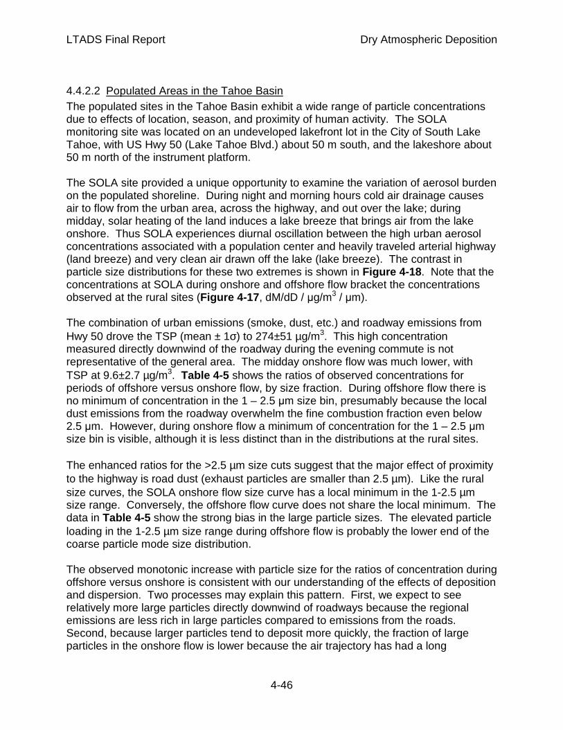
LTADS Final Report Dry Atmospheric Deposition
4-46
4.4.2.2 Populated Areas in the Tahoe Basin The populated sites in the Tahoe Basin exhibit a wide range of particle concentrations due to effects of location, season, and proximity of human activity. The SOLA monitoring site was located on an undeveloped lakefront lot in the City of South Lake Tahoe, with US Hwy 50 (Lake Tahoe Blvd.) about 50 m south, and the lakeshore about 50 m north of the instrument platform. The SOLA site provided a unique opportunity to examine the variation of aerosol burden on the populated shoreline. During night and morning hours cold air drainage causes air to flow from the urban area, across the highway, and out over the lake; during midday, solar heating of the land induces a lake breeze that brings air from the lake onshore. Thus SOLA experiences diurnal oscillation between the high urban aerosol concentrations associated with a population center and heavily traveled arterial highway (land breeze) and very clean air drawn off the lake (lake breeze). The contrast in particle size distributions for these two extremes is shown in Figure 4-18 . Note that the concentrations at SOLA during onshore and offshore flow bracket the concentrations observed at the rural sites (Figure 4-17 , dM/dD / µg/m3 / µm). The combination of urban emissions (smoke, dust, etc.) and roadway emissions from Hwy 50 drove the TSP (mean ± 1σ) to 274±51 µg/m3. This high concentration measured directly downwind of the roadway during the evening commute is not representative of the general area. The midday onshore flow was much lower, with TSP at 9.6±2.7 µg/m3. Table 4-5 shows the ratios of observed concentrations for periods of offshore versus onshore flow, by size fraction. During offshore flow there is no minimum of concentration in the 1 – 2.5 µm size bin, presumably because the local dust emissions from the roadway overwhelm the fine combustion fraction even below 2.5 µm. However, during onshore flow a minimum of concentration for the 1 – 2.5 µm size bin is visible, although it is less distinct than in the distributions at the rural sites. The enhanced ratios for the >2.5 µm size cuts suggest that the major effect of proximity to the highway is road dust (exhaust particles are smaller than 2.5 µm). Like the rural size curves, the SOLA onshore flow size curve has a local minimum in the 1-2.5 µm size range. Conversely, the offshore flow curve does not share the local minimum. The data in Table 4-5 show the strong bias in the large particle sizes. The elevated particle loading in the 1-2.5 µm size range during offshore flow is probably the lower end of the coarse particle mode size distribution. The observed monotonic increase with particle size for the ratios of concentration during offshore versus onshore is consistent with our understanding of the effects of deposition and dispersion. Two processes may explain this pattern. First, we expect to see relatively more large particles directly downwind of roadways because the regional emissions are less rich in large particles compared to emissions from the roads. Second, because larger particles tend to deposit more quickly, the fraction of large particles in the onshore flow is lower because the air trajectory has had a long

LTADS Final Report Dry Atmospheric Deposition
4-47
residence time over the lake, and is not dominated by the very local emissions, and thus contains a lower fraction of short-lived (larger) particles. Data discussed in the next section indicate that both processes contribute to the observed difference.
4.4.3 Spatial Variation between Lakeshore and mid-l ake Areas The strong difference between the composition of air under different flow regimes observed at SOLA (see previous section) suggests that air flowing from land out onto the lake is not simply diluted, but undergoes transformation by selective deposition of terrestrial pollutants and mixing with regional "background" air. This pattern suggests that there is a zone of terrestrial influence near shore, which grades outward to a well-mixed mid-lake environment. In order to evaluate the extent of land-lake interaction a series of experiments were conducted using instruments mounted on the U.C. Davis research vessel RV Frantz. The basic experimental design was to sample mid-lake air and shore-zone air by running in open water and cruising the shoreline during evening and morning hours when downslope air drainage drives offshore flow. The pollutant measurements taken on the boat included NOy recorded continuously (a few seconds time resolution) and a CI-500 particle counter collecting particle size data with a resolution of 1 minute. The NOy is interpreted as a tracer for NOx-producing combustion (primarily motor vehicles), fine particles are interpreted as combustion (i.e. " smoke"), and coarse particles are interpreted as road dust. Cruising at about 4 knots (0.5 m / sec) produced transect data with spatial resolution on the order of 120 m. Sampling under stable meteorological conditions during downslope flow, the RV Frantz night-morning data focus on the strong downslope flow regimes, and represent the peak conditions for terrestrial effects on the lake. Limited data taken during well mixed periods show that the shore - mid-lake contrast is much weaker at midday or when regional winds mix air throughout the Tahoe Basin. The evening and morning courses were very similar, with each consisting of an outbound leg from Tahoe City crossing open waters toward the north east shore near Incline Village and a return leg following close to the north shore. The morning outbound leg differed from the evening outbound leg in that it passed farther south of Stateline Point, and ended a little farther south near the east shore.

LTADS Final Report Dry Atmospheric Deposition
4-48
Figure 4-18. Extreme results in the diurnal aerosol cycle at SOLA. The difference in TSP concentration is a factor approximately 30:1, necessitating the logarithmic scale in the plot. The shapes of the distributions indicate a bias toward large particles during offshore flow (see Table 4-5).
Table 4-5. Ratio of mean offshore to mean onshore size-resolved and total aerosol concentrations for the data from Figure 4-18.
SIZE_BIN OFFSHORE / ONSHORE0.5 - 1 um 8.21 - 2.5 um 11.32.5 - 5 um 20.25 - 10 um 29.8
10 - 25 um 33.9>25 um 31.9PM25 10.8PM10 26.7TSP 25.2
COARSE 29.7LARGE PM 27.0
1 108 9 2 3 4 5 6 7 8 9 2 3 4
D µm
0.1
1
10
6789
2
3
4
5678
2
3
4
56789
2
3
4
δM /
δD µ
g/m
3/µ
m
Beach Near SOLA
3/11/2004
0.0
0.1
0.2
0.3
0.4
0.5
0.6
0.7
0.8
0.9
1.0
CU
MU
LAT
IVE
MA
SS
FR
AC
TIO
N
SIZE DISTRIBUTION - ONSHORE FLOW (3-5 pm) SIZE DISTRIBUTION - OFFSHORE FLOW (6-8 pm) CUMULATIVE FRACTION - 3-5 pmCUMULATIVE FRACTION - 6-8 pm
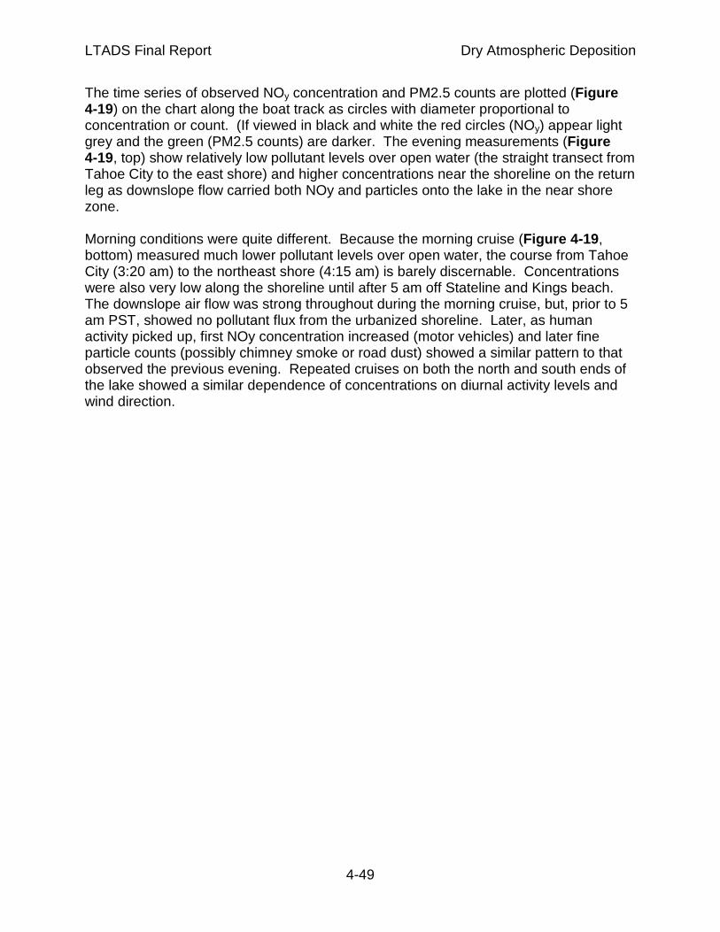
LTADS Final Report Dry Atmospheric Deposition
4-49
The time series of observed NOy concentration and PM2.5 counts are plotted (Figure 4-19) on the chart along the boat track as circles with diameter proportional to concentration or count. (If viewed in black and white the red circles (NOy) appear light grey and the green (PM2.5 counts) are darker. The evening measurements (Figure 4-19, top) show relatively low pollutant levels over open water (the straight transect from Tahoe City to the east shore) and higher concentrations near the shoreline on the return leg as downslope flow carried both NOy and particles onto the lake in the near shore zone. Morning conditions were quite different. Because the morning cruise (Figure 4-19 , bottom) measured much lower pollutant levels over open water, the course from Tahoe City (3:20 am) to the northeast shore (4:15 am) is barely discernable. Concentrations were also very low along the shoreline until after 5 am off Stateline and Kings beach. The downslope air flow was strong throughout during the morning cruise, but, prior to 5 am PST, showed no pollutant flux from the urbanized shoreline. Later, as human activity picked up, first NOy concentration increased (motor vehicles) and later fine particle counts (possibly chimney smoke or road dust) showed a similar pattern to that observed the previous evening. Repeated cruises on both the north and south ends of the lake showed a similar dependence of concentrations on diurnal activity levels and wind direction.

LTADS Final Report Dry Atmospheric Deposition
4-50
Figure 4-19. Night and morning patterns of pollution, on north end of Lake Tahoe.
Figure 4-20 shows particle size data from a morning cruise on the south end of Lake Tahoe. In that cruise three distinct regimes were observed: air drainage from the SE shore (Zephyr Cove to Tahoe Keys) showed strong pollutant flux; air drainage from the largely unpopulated shoreline between Camp Richardson and Emerald Bay lacked strong pollutant signatures; and air encountered traversing the lake from Emerald Bay back to Zephyr Cove showed evidence of dilute accumulated pollution.

LTADS Final Report Dry Atmospheric Deposition
4-51
Figure 4-20. Particle size distributions observed during a morning cruise on the south end of Lake Tahoe. Strong pollutant flux was observed from the South Lake Tahoe area, while drainage air along the unpopulated shoreline was cleaner than that at mid-lake.
The particle size distribution from the "clean" shoreline approximates the "background" as measured at the remote sites (Figure 4-17 ), but the urban shore zone concentrations are much lower than the offshore flow observed at SOLA. This discrepancy suggests that there is strong dilution from shoreline to our monitoring path (approximately 0.3 km from the shoreline along most of the developed shoreline). The next section addresses this question.
4.4.4 Dilution and Deposition of Roadway Emissions Because the SOLA site data represents both the well-mixed lake environment (during onshore flow) and the strong local effect of Hwy 50 traffic and other urban emissions (during offshore flow) it is desirable to understand the local particle concentration gradients. Because human activity and development is generally near the shoreline and emissions from roadways may impact several of the LTADS monitoring sites we
1 100.8 0.9 2 3 4 5 6 7 8 9 20 30 40
D µm
0
1
2
3
4
5
6
7
δM /
δD µ
g / m
3 / µm
SOUTH SHORE ZONE - MORNING CRUISE - 8/19/03
UNPOPULATED SHORELINEOPEN WATERURBAN SHORELIINE

LTADS Final Report Dry Atmospheric Deposition
4-52
made measurements to better understand the gradients between the roads and the shoreline. The roads appeared to be a major source of particles in the Tahoe Basin, but, as expected, within a short distance downwind the observed concentrations decreased and size distributions changed significantly compared to those measured near the roadside. During downslope flow on the evening of March 11, 2004, three optical particle counters were operated near the SOLA site at distances of 6, 16, and 100 m from the nearest traffic lane of Highway 50. Estimated mass concentrations, calculated from the particle counts, declined significantly with downwind distance (Figure 4-21 ). The observed decrease of concentration with downwind distance is further characterized by fitting power functions of the form C=C0 e
-K(x) to the data, where C is concentration at distance x downwind, C0 is concentration (extrapolated) at the nearest traffic lane, and K is the “depletion coefficient” for the selected particle size class. A constant depletion coefficient implies an equal fractional decline in concentration per unit distance of transit downwind from the road. However, the observed decline is due to the combined effects of deposition and dispersion and their relative influences will change with distance. For the purpose of the following analysis we assumed the particle dispersion is effectively size-independent over the horizontal scale of this experiment (about 100 m). In general, for the different size fractions any differences in upwind concentration or vertical profiles of concentration would cause the ground level concentrations to decline at different rates with downwind distance (because the same vertical mixing would incorporate different aloft concentrations into the plume). However, to the contrary, we assumed that over this distance the local emissions of particles from the roadway overwhelmed the background particle concentrations in all size fractions. To investigate the roles of dispersion and deposition we compared the depletion coefficients for the different size fractions as calculated from the observed particle counts. Our general understanding of deposition (see Fig. 4-13 ) suggests that the loss of fine particles (~1 µm) over such a short transit should be negligible. The smallest depletion coefficient (for particles of 0.5-1 or 1-2.5 µm diameter) was attributed entirely to dispersion and was assumed to represent the rate of dispersion for all size fractions. Thus, for each size fraction, subtracting this dispersion coefficient from the depletion coefficient provided a “deposition” coefficient. For each size fraction this deposition coefficient was used to calculate the fraction of particles that would remain in the atmosphere at the SOLA site and at the beach (50 and 100 m from the road). Table 4-6 shows the results of such a treatment for morning and evening experiments near SOLA. Although the conditions (traffic, temperature, humidity and wind speeds) differed between the two experiments, both were under down-slope flow conditions and the patterns of concentration were similar. Similar fractions of particles were predicted to remain in the atmosphere and the variation in ratios of predicted atmospheric survival of PM at the beach compared to at SOLA (“beach/SOLA ratio”) differed between size fractions in a similar manner. The 0.5 – 1 and 1 – 2.5 µm fractions appear to have

LTADS Final Report Dry Atmospheric Deposition
4-53
similar rates of depletion, the depletion is greater for the coarse particles (2.5 – 5 and 5 -10 µm), and depletion is much greater for particles larger than 10 µm. We expect that the local roadway emissions of both coarse and large particles dominate concentrations downwind and that for these size fractions any effects of possible differences in upwind concentrations or vertical profiles would be minimal. Thus, the difference in depletion for coarse and large particles should be a measure of their loss by deposition over this short distance. On the other hand, there is a greater potential for upwind particle concentrations to influence the apparent rate of depletion for the fine particles, so conclusions about the relative losses for fine versus coarse particles are less certain.
Figure 4-21. Change in particle concentrations observed at, and fitted power functions for, the area downwind of Highway 50 at SOLA on the evening of March 11, 2004. Dotted lines are 95% confidence bounds for the fits.
0 20 40 60 80 100DISTANCE m
0
1
2
3
4
µg m
3
0.5 - 1.0 µm
0 20 40 60 80 100DISTANCE m
0
2
4
6
8
10
12
µg m
3
1.0 - 2.5 µm
0 20 40 60 80 100DISTANCE m
020406080
100120140160180
µg m
3
2.5 - 5.0 µm
0 20 40 60 80 100DISTANCE m
0
100
200
300
400
500
600
µg m
3
5 - 10 µm
0 20 40 60 80 100DISTANCE m
0200400600800
100012001400
16001800
µg m
3
10 - 25 µm
0 20 40 60 80 100DISTANCE m
0
100
200
300
400
500
600
µg m
3
> 25 µm

LTADS Final Report Dry Atmospheric Deposition
4-54
Table 4-6. Computation of size-resolved particle loss between SOLA and the lakeshore for dispersion experiments on afternoon of March 11 and morning of March 12, 2004.
These data, taken together with the findings of the near-shore boat sampling discussed in Section 4.5.3 indicate that downslope winds deliver concentrated particle plumes to the lake from the heavily developed urban and residential portions of the lake shore, and that these plumes diminish in intensity fairly quickly with increasing distance from the source. Although there are no simultaneous off-shore size-resolved data to compare with these experiments, a rough sense of the scale of off-shore transport can be found by applying the concentrations and apparent rate of reduction from these experiments to the concentrations observed on the lake under similar meteorological conditions (Figures 4-19 and 4-20 ). Concentrations observed in the urban shore zone would be reached about 250 m offshore, and concentrations near those measured in open water would be reached about 500 m from shore. Although highly uncertain due to the mismatched data, this calculation suggests that the shore zone effect is limited to a few hundred meters to 1 km, and shows consistency between the roadside and on-lake results.
4.4.5 Estimated Particle Number and Deposited Fract ion In addition to providing nutrients for algae that reduce lake clarity, atmospheric deposition also adds inert (non-soluble) particles to the lake. These inert particles scatter light within the water column with an optical efficiency that is strongly dependent on their size and chemical composition. The numbers of these inert particles within the aerosol mass is not well known, but LTADS obtained some particle count data during short-term monitoring. The particle count information, when combined with particle chemical data from the LTADS and IMPROVE filter records, can be used to generate a rough estimate of the optical efficiency characteristics of deposited particles. Count and
STAGETOTAL
REDUCTION COEFF
DISPERSION COEFF
DEPOSITION COEFF
SURVIVING FRACTION AT SOLA (50 m)
SURVIVING FRACTION AT
BEACH (100 m)BEACH / SOLA
RATIO UNCERTAINTY
MAR 11 - PM
0.5 - 1 um -0.171 -0.127 -0.044 0.843 0.818 0.97 3%1 - 2.5 um -0.127 -0.127 0.000 1.000 1.000 1.00 1%2.5 - 5 um -0.286 -0.127 -0.158 0.538 0.482 0.90 7%5 - 10 um -0.464 -0.127 -0.337 0.268 0.212 0.79 3%
10 - 25 um -1.122 -0.127 -0.995 0.020 0.010 0.50 1%>25 um -1.027 -0.127 -0.900 0.030 0.016 0.54 6%
MAR 12 - AM
0.5 - 1 um -0.124 -0.124 0.000 1.000 1.000 1.00 2%1 - 2.5 um -0.165 -0.124 -0.042 0.850 0.826 0.97 0%2.5 - 5 um -0.269 -0.124 -0.145 0.567 0.513 0.90 6%5 - 10 um -0.416 -0.124 -0.292 0.318 0.260 0.82 3%
10 - 25 um -0.916 -0.124 -0.792 0.045 0.026 0.58 1%>25 um -0.916 -0.124 -0.792 0.045 0.026 0.58 5%

LTADS Final Report Dry Atmospheric Deposition
4-55
mass data averaged over a week at SOLA are shown in Figure 4-22 . The left vertical scale, dN/dD, describes the change in particle number (N) per change in particle diameter (D), indicating relative numbers of particles by size bins of particle diameter. In this example, near and downwind of highway 50 at the SOLA site in South Lake Tahoe the fine fraction (D < 2.5 µm) contained over 95% of the particle numbers but less than 10% of the mass. The coarse fraction contained a few percent of the particle count and about 45% of the mass. Large particles (> 10 µm) comprised about one percent of the particle number and about 50% of the total mass. Figure 4-22. Mean particle number and cumulative mass and number distributions at SOLA 9/2-9/2003. Arrows denote filter sample size ranges in the LTADS measurements. Fines dominate in numbers; large particles dominate in mass.
1 100.7 0.80.9 2 3 4 5 6 7 8 9 20 30 40 50
D µm
1
10
100
1000
10000
100000
1e+006
1e+007
δN /
δD
PM2.5 "COARSE" "LARGE"
SOLA 9/2-9/2003
0.0
0.1
0.2
0.3
0.4
0.5
0.6
0.7
0.8
0.9
1.0
CU
MU
LAT
IVE
FR
AC
TIO
N
dN/dDCUMULATIVE MASSCUMULATIVE NUMBER

LTADS Final Report Dry Atmospheric Deposition
4-56
The size ranges of concern for light scattering by inert particles in the lake fall in the PM2.5 fraction. Within that fraction, there are three general classes of chemical materials based on their effect on lake turbidity:
1. soluble species (e.g. sulfates and nitrates) that dissolve into the lake water and have no residual optical effect;
2. organic materials which, although largely insoluble, have refractive indices near that of water, and thus are optically unimportant; and
3. inert materials (e.g. soot and soil minerals) that persist within the water column after deposition and contribute to the turbidity of the lake.
Computing the inert fraction of deposited particle numbers requires first converting particle mass as measured with the filters to estimated particle numbers, then allocating the numbers to the three particle types listed above. The first five panels of Figure 4-23 illustrate the relationship between observed particle counts and particle mass estimated from those count observations. For the particle size categories spanning a relatively small range of particle diameters, mass and particle counts are closely related. For fine or large particles, or even for coarse particles the observed particle mass appears to provide a reasonably consistent estimate of particle numbers. However, if fine and coarse are combined and examined together as PM10, or, especially if large particles are also included (as in the definition of TSP), then there is very little relationship between particle mass and numbers. The final panel in Figure 4-23 compares the scatter of 1-hour BAM TSP measured mass (µg/m3) versus total particle counts. Because there is such a large range of counts between the 0.5-1 µm and 1-2.5 µm size bins, the chemical allocation of PM2.5 is subdivided based on size distributions for "typical" aerosols to estimate where each chemical type lies in the size-number distribution. The allocation of chemical species for LTADS is based in part on limited size-resolved chemical data available from Mt. Lassen (Figure 4-24 ). Although Lassen is a more remote site it provides size resolved and chemically speciated data not otherwise available in the Sierra Nevada at a similar elevation and distance from the Pacific. Based on location Lassen is subject to similar meteorological regimes and potential transport from populated areas in coastal and valley areas to the west and from Asia. By that reasoning we expect a similar chemical speciation at Lassen despite a somewhat more aged air mass, less urban influence, and lower concentrations at Lassen. An observed strong similarity between Lassen air quality and that in less-developed areas of the Tahoe basin (e.g. Bliss State Park) means that, lacking Tahoe specific data, Lassen is a reasonable analog for typical, basin-wide conditions. Moreover, size distributions by species should be similar because the origins of the materials play a large role in their particle sizes - soil dust is dominated by mechanically produced particles, thus it will tend to large particle sizes; combustion products are produced chemically and tend to smaller sizes.
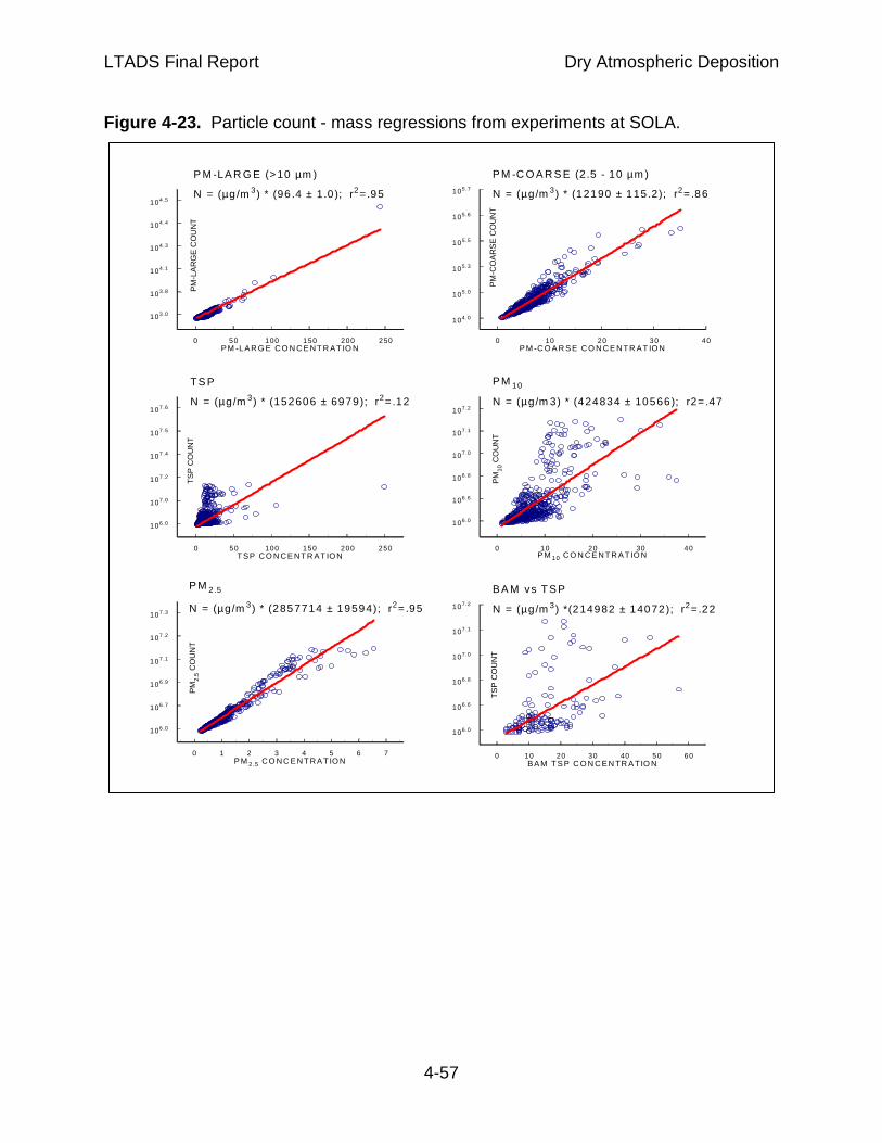
LTADS Final Report Dry Atmospheric Deposition
4-57
Figure 4-23. Particle count - mass regressions from experiments at SOLA.
0 50 100 150 200 250PM -LAR G E C O N C E N T R AT IO N
103.0
103.8
104.1
104.3
104.4
104.5P
M-L
AR
GE
CO
UN
T
P M -LA R G E (>10 µm )
N = (µg/m 3 ) * (96 .4 ± 1.0 ); r2=.95
0 10 20 30 40P M -C O A R SE C O N C E N T R AT IO N
104.0
105.0
105.3
105.5
105.6
105.7
PM
-CO
AR
SE
CO
UN
T
P M -C O A R S E (2.5 - 10 µm )
N = (µg/m 3 ) * (12190 ± 115.2); r2=.86
0 50 100 150 200 250T SP C O N C E N T R AT IO N
106.0
107.0
107.2
107.4
107.5
107.6
TS
P C
OU
NT
TS P
N = (µg/m 3 ) * (152606 ± 6979); r2=.12
0 10 20 30 40P M 10 C O N C E N T R AT IO N
106.0
106.6
106.8
107.0
107.1
107.2
PM
10 C
OU
NT
P M 10
N = (µg/m 3) * (424834 ± 10566); r2= .47
0 1 2 3 4 5 6 7P M 2 .5 C O N C E N T R A T IO N
106.0
106.7
106.9
107.1
107.2
107.3
PM
2.5 C
OU
NT
P M 2.5
N = (µg/m 3 ) * (2857714 ± 19594); r2=.95
0 10 20 30 40 50 60BA M T S P C O N C EN TR A TIO N
106.0
106.6
106.8
107.0
107.1
107.2
TS
P C
OU
NT
B A M vs T S P
N = (µg/m 3 ) *(214982 ± 14072); r2=.22

LTADS Final Report Dry Atmospheric Deposition
4-58
Figure 4-24. Size distributions and mass fractions of various elements at Mt. Lassen.
Solid line = mass fraction, dashed line = cumulative fraction. S represents soluble species; Zn and K inert combustion products; Si, Al, and Fe represent inert soil components. Vertical lines mark limits of the 0.5 -1 µm and 1 - 2.5 µm size ranges.
Using a combination of the regressions of PM2.5 particle counts versus mass (Figure 4-23) and inferences drawn from the Mt. Lassen data (Figure 4-24 ) a species allocation scheme was developed for the LTADS PM2.5 data. The results of applying this scheme to SOLA data are shown in Table 4-7 .

LTADS Final Report Dry Atmospheric Deposition
4-59
Table 4-7. Allocation of particle types to seasonal data from SOLA.
The table shows that the particles greater than 1 µm constitute less than 10 percent of the PM2.5 count, with over 90 percent below that size. The table also shows that the relative composition of PM2.5 varies, with inert particles a fairly constant fraction (33-39 percent), while solubles vary seasonally, from a low near 10 percent in winter to more than double (24 percent) in summer. Organic particles also show significant seasonality, varying between a winter peak of over half (56 percent) to a summer minimum (37 percent). The last columns in Table 4-7 show the concentration model converted into particle counts. The optical implications of these calculations are that strongly scattering fine inert particles constitute about 30 percent of PM2.5 particles, regardless of season, while most of the seasonal variation is in the optically weak organic and soluble particles. These calculations suggest that rough estimation of the inert particle deposition load can be done by simple linear adjustment of the estimated particle number based on the PM2.5 regression in Figure 4-24 .
91.2% 8.8%
SOLA ANNUAL MEAN TYPE 0.5 - 1.0 um 1.0 - 2.5 um all PM2.5 0.5-1 um COUNT 1 - 2.5 um COUNTSOIL 1122 INERT 10.2% 26.1% 36.4% 2360787 581300 31%EC 1726 SOLUBLE 9.2% 7.3% 16.5% 2126856 161464 24%OC 2955 OM 15.6% 31.6% 47.2% 3585128 703299 45%SO4 574NO3_ 389MF 8841 PERCENT 35.0% 65.0% 100.0% 8072770 1446063
SOLA APR-OCTSOIL 1166 INERT 10.0% 29.0% 39.0% 1861900 523776 31%EC 1258 SOLUBLE 12.2% 9.6% 21.8% 2283354 173345 32%OC 1952 OM 12.9% 26.3% 39.2% 2419717 474679 37%SO4 711NO3_ 294MF 7173 35.1% 64.9% 100.0% 6564971 1171800
SOLA MAY-SEPSOIL 1120 INERT 9.7% 28.9% 38.7% 1735421 499949 30%EC 1138 SOLUBLE 13.4% 10.5% 23.9% 2392770 181652 35%OC 1749 OM 12.4% 25.1% 37.4% 2208371 433219 35%SO4 754NO3_ 279MF 6859 35.5% 64.5% 100.0% 6336562 1114819
SOLA NOV-MARSOIL 1040 INERT 10.6% 23.0% 33.6% 3345836 705868 31%EC 2594 SOLUBLE 6.1% 4.8% 10.8% 1919790 145745 16%OC 4812 OM 18.3% 37.3% 55.6% 5817624 1141250 53%SO4 321NO3_ 565MF 12168 35.0% 65.0% 100.0% 11083250 1992863
TYPICAL COUNT %FRACTION OF PM2.5
PM2.5 ng/m3 COUNT
FRACTION

LTADS Final Report Dry Atmospheric Deposition
4-60
4.5 Key Assumptions and Resultant Bias Identified in this section are key assumptions used in the estimation of deposition velocities and, subsequently, pollutant deposition. They are approximately ordered by the magnitude of the bias they may introduce into the estimates of deposition. Some assumptions clearly will introduce a positive bias. This was intentional so that the contribution of atmospheric deposition in the TMDL would not be underestimated.
4.5.1 Assumptions Likely to Introduce the Largest B ias The assumption that concentrations of PM measured over land (at Sandy Way in SLT, Lake Forest on the northwest shore, and Thunderbird on the east shore) are also representative of concentrations over mid-Lake areas would likely introduce a very significant positive bias in estimated deposition rates for PM because the urban measurement sites are significantly impacted by local PM emission sources. Based on the brief experiments described in Section 4.4 and expectations regarding patterns of deposition and dispersion, significant decreases in downwind PM concentrations are likely over some areas of the Lake. Nevertheless, such estimates are useful because they provide a reference and upper bound on the annual dry deposition. Thus they are presented for reference in Appendix L. Peer reviewers commented that this conservative assumption reduced the utility of the estimates. We agree and in particular were concerned that comparisons of estimates of dry deposition and estimates of other inputs to the Lake would be difficult because of the bias included in that previous estimate. To provide a more realistic estimate of deposition, the measured concentrations of PM in the urban areas were assumed to be depleted by a modest amount over the Lake. For several reasons the nitrogen concentrations were not assumed to be depleted. Compared to PM, nitrogen species (dominated by ammonia and nitric acid) are more regionally mixed and the nitric acid is formed in the atmosphere rather than directly emitted. Because the ammonia gas and nitric acid gas appear to be mixed through deeper layers, it is expected that vertical mixing over the Lake will tend to refresh surface concentrations of those species over the Lake. The vertical mixing is generally enhanced during hours of offshore flow because at those times the Lake is usually warmer than the air flowing onto it. Similarly, because ammonia and nitric acid are more regionally dispersed than the PM, horizontal dispersion downwind of the urban area monitoring sites is much less of an issue. Thus, nitrogen species concentrations measured at the urban sites are expected to be relatively similar to those on the Lake. The deposition estimates provided here assume a modest depletion in concentrations of PM and phosphorus over the Lake compared to concentrations observed at the urban monitoring sites (Sandy Way and Lake Forest). For estimating the depletion of concentration the observations at Thunderbird were utilized as an indicator of concentrations on the Lake. The Thunderbird site is located far from busy local roadways and experiences onshore flow for many hours of the day. In contrast the

LTADS Final Report Dry Atmospheric Deposition
4-61
urban sites (Sandy Way and Lake Forest) are relatively close to emission sources and are subject to some urban influences regardless of wind direction. Depletion of PM concentrations was assumed for the north and south Lake quadrants only. For the north quadrant the concentration of each size fraction was reduced from the Lake Forest concentration by 25% of the difference between the Lake Forest and Thunderbird concentrations. The calculation of concentration for the south quadrant was analogous, but used PM concentrations from Sandy Way instead of from Lake Forest. The reduction in PM concentration was calculated independently for each of the three size fractions. As a result, the reductions in concentration were greatest for the large particles and least for the fine particles, reflecting the fact that the observed PM_large concentrations were much lower at the Thunderbird site compared to the urban sites. Differences were much less for the PM2.5 concentrations. The validity of these assumptions concerning spatial and temporal variations in particle mass concentrations and particle size distributions over the Lake can be partially evaluated against the particle counts obtained during the short term targeted studies (Section 4.4). Although those are of limited duration and based upon particle counts instead of measured mass, those studies do support the expected decrease in concentration out over the Lake. However, more quantitative extrapolations from this data are not warranted because those studies are temporally and spatially limited, and represent only snap shots of conditions during a few seasons.
4.5.2 Assumptions Likely to Introduce Moderate Posi tive Bias The assumptions concerning the spatial variations of concentration are thought to be the largest source of uncertainty in the deposition estimates. Relatively modest bias may be introduced by the additional assumptions listed below. • A modest overestimation of dry deposition may result from calculating dry deposition
as occurring during all periods, including those with precipitation. Thus, a potential positive bias is included in the estimates of dry deposition by over-counting hours of dry deposition. During 2003, trace (or more) precipitation was measured at Incline Creek for 6% of hours (503) and 25% of days (92). However, this overestimation is moderated by the manner concentrations were treated. Average concentrations reported for each season were based upon all available two-week data, including periods of precipitation with presumably lower concentrations.
• The distributions of particle sizes within each of the three measured PM size
categories (or bins) were not known. Assumed characteristic particle diameters were utilized for calculation of lower, central, and upper bound estimates of deposition velocity. For this purpose, the assumed particle diameter used to represent the rate of mass deposition for a size bin should be skewed toward the upper bound of the bin; first, because the larger particles contain a disproportionately large fraction of that bin’s mass and, second, because the deposition velocity generally increases with particle size (especially within the coarse and large particles categories). For the lower and upper bound estimates, extreme

LTADS Final Report Dry Atmospheric Deposition
4-62
particle diameters were chosen to ensure the appropriate bias in the calculated mass deposition rates for each bin. For the central estimates the assumed particle diameter for PM_large is expected to provide a substantial positive bias and the assumed diameter for PM_coarse is expected to be approximately neutral with respect to any bias. The assumed particle diameters for each size fraction are listed in Table 4-8 for the lower, central, and upper estimates.
The characteristic diameters assumed for the upper estimate very obviously overstate the size of PM_fine and PM_coarse and based on the particle count observations also overstate the size of PM_large. Clearly, PM-fine must include particles smaller than 2.5 µm and the assumption of 2.5 µm as the characteristic size must overestimate the size. Similarly for PM_coarse (2.5 µm < PM diameter < 10 µm) an assumed diameter of 10 µm must overestimate the characteristic size and thus the deposition velocity of PM-coarse. For PM_large (TSP – PM10), a characteristic diameter of 25 µm was assumed for the upper estimate. While there is no upper limit defined on the diameter of TSP or PM_large, the available data suggests that 25 µm is an overestimate of the characteristic particle size of PM_large, and thus will overestimate the deposition velocity for PM-large. Although larger particle sizes have been observed in urban areas of southern California by Lu, et al. (2003), the available LTADS data suggest that particles larger than 25 µm contribute a very small fraction of the mass of PM_large over Lake Tahoe. This conclusion is based both on the size resolved optical particle counts and on comparison of mass in PM_coarse versus PM_large from the TWS data. Thus, there is reasonable certainty that the assignment of 25 µm as the characteristic size for large particles is sufficiently conservative to represent the worst case condition at the shoreline of the Lake. Applying these same particle sizes for calculations at mid-Lake should be yet more conservative as an upper bound of deposition to the Lake.

LTADS Final Report Dry Atmospheric Deposition
4-63
Table 4-8. Assumptions regarding characteristic particle sizes and maximum allowable aerodynamic conductance.
Assumed Diameter for Particle Size Fraction (µm) Type of Estimate Fine
(PM2.5) Coarse
(PM10 – PM2.5) Large
(TSP – PM10)
“Cap” on 1/Ra (cm/s) (max aerodynamic
conductance)
Lower 1 2.5 10 3
Central 2 8 20 6
Upper 2.5 10 25 10
4.5.3 Assumptions Expected to Introduce a Smaller P ositive Bias Several assumptions are expected to cause a small positive bias in the estimated deposition rates. These biases are thought to be insignificant compared to other uncertainties.
• Deposition velocities of the gases HNO3 and NH3 were approximated as the inverse of the aerodynamic resistance Ra (assumed Ra >> Rb and Rc ~ 0). This is a standard assumption for deposition of very reactive or soluble gases over water (e.g., Valigura, 1995) but may produce a small positive bias in deposition velocity when Ra is very small.
• As discussed previously, small values of aerodynamic resistance calculated in the near-shore zone during offshore flow are known to be unrealistic and thus were not used in calculation of the deposition estimates. The assumption of a logarithmic wind profile (modified by stability effects) is valid at heights above 50 times the aerodynamic roughness length scale (Z0) but not for heights that are of the same order as Z0. Thus, for the near-shore zone during offshore winds it was necessary to set a maximum value for the inverse of aerodynamic resistance. Maximum values were assigned as 3, 6, and 10 cm/s for the lower bound, central, and upper bound estimates. These were used as the maximum deposition velocity for the gases (ammonia and nitric acid) and were also used in calculation of the deposition velocity for particles. The assumption of a 6 cm/s cap on 1/Ra for the central estimate case is rather generous maximum and is likely to result in a positive bias in deposition velocities of gases and particles for some periods in the near-shore zone. But note that it is only applied to a limited area of the Lake, and only during offshore winds, so the effect on average deposition rates to the Lake is expected to be small. The cap on 1/Ra (10 cm/s) used for the upper limit estimate was chosen as the largest value found in the literature for any modeling of gaseous deposition and it is likely more than double the actual maximum deposition based on observed rates for SO2 to water surfaces (Whelpdale and Shaw, 1974; Sehmel, 1980). The cap of 10 cm/s is expected to cause a positive bias in the estimates of deposition velocity for gaseous species, PM2.5 and to a lesser extent for PM_coarse but will have little effect on deposition estimates for PM_large.

LTADS Final Report Dry Atmospheric Deposition
4-64
• Increased turbulence due to roughness over land (assumed to be 1 m) was assumed to be advected to 1 kilometer offshore. The deposition velocity in this near-shore zone was calculated as the average of the over-water and near-shore deposition velocities. Calculation of deposition velocity assumed Z0 of 1 m at the shoreline and Z0 as a function of wind speed over open water. This is the arithmetic equivalent of a linear decay of the shoreline deposition velocity to the lower open water deposition velocity at a distance of 1 km offshore. Thus, for estimation of Ra near the shoreline during periods of offshore winds, an appropriately higher estimate of deposition velocity (than would be provided by the standard over-water formulations) was provided by adjusting Z0 to appropriate values for forested areas. However, the use a Z0 of 1 m caused the maximum deposition velocity to be invoked for the near-shore zone. This may result in some over estimation of deposition in this limited area.
• The calculated effects of atmospheric stability on turbulence and deposition
velocity were based on the observed hourly air and water temperatures. Implicit is an assumption that the temperature at the air-water interface equals the measured water temperature (at 2 cm depth). If winds are calm this assumption is likely to overestimate the temperature at the water interface at night and underestimate it during the day. Because calms are more frequent at night the overall bias would be a small overestimation of surface temperature and a bias toward overstating instability. This very small effect would cause a very slight overstating of the deposition velocities.
4.5.4 Assumptions Presumed to be Approximately Bias Neutral The following assumptions were made as part of the analysis and are intended to support reasonable estimates of the rate of deposition. Though they may introduce a bias, the direction (sign) is not readily apparent.
• Neglecting the effects of particle growth may introduce a small negative bias in total particle mass deposition. For large and very small particles (< 0.5 µm), hygroscopic increase in particle size over the Lake would increase deposition velocities, so neglect of this particle growth may under estimate deposition rates. However, for the minor fraction of particles in the 0.5 – 1 µm size range, deposition velocity would be decreased with an increase in particle size. For LTADS, a small negative bias is expected because most of the observed mass is in the size ranges for which deposition velocities are increased with particle diameter.
• Neglecting the effects of breaking waves and spray underestimates annual
deposition rates for particles at Lake Tahoe by less than one percent. See Section 4.3.2.4 for the background information and observations that support this quantification.
• Aerodynamic roughness length, Z0, over open water was calculated based upon
wind speed as shown in equation 4.9 . This is expected to be bias neutral.

LTADS Final Report Dry Atmospheric Deposition
4-65
4.6 Variations in Deposition Velocity The deposition velocities calculated from the meteorological data in this analysis exhibited significant temporal variation as well as spatial variation between near-shore and open-water areas. The significant temporal variation in calculated deposition velocities was associated mainly with the daily variation in wind speed and direction. In contrast, relatively small differences were found between the averaged deposition velocities calculated from the meteorological data of the different sites.
4.6.1 Temporal Variations in Deposition Velocity Figures 4-25 through 4-27 illustrate the diurnal variations in deposition velocities based on the meteorological data from specific sites. The deposition velocities are averaged by hour of day across a seasonal period to provide a 24-hour representation of the diurnal course of deposition velocity. The averaging masks day-to-day differences in meteorology, highlighting the effects of the slope flows and land-Lake breezes that tend to repeat at similar times each day. Deposition velocities shown are examples based on meteorological data from a few specific sites. The complete list of sites included the U.S. Coast Guard pier on the northwest shore (about 3 km northeast of Tahoe City), Tahoe Vista pier on the north shore west of Incline Village, Cave Rock boat launch on the east shore, Timber Cove pier in the City of South Lake Tahoe, Sunnyside pier on the west shore (about 3 km south of Tahoe City), and TDR1 and TDR2 buoys (respectively located approximately about 3 km east of Meeks and Emerald Bays). The estimates of deposition velocity for soluble and reactive gases (shown in Figures 4-25 and 4-26 ) are directly dependent on meteorological conditions because they are estimated as the inverse of the aerodynamic resistance. Deposition velocities for open water areas (and for the near-shore zone during onshore flow) are shown in Figure 4-25 and are based on meteorological data from the Coast Guard and Timber Cove piers. The estimates for the mid-Lake open water areas are independent of wind direction. Their daily variation is due primarily to changes in wind speed and secondarily to changes in the air-water temperature difference. The summer average of hourly deposition velocity for gases at the U.S. Coast Guard pier is less than 0.2 cm/s for two hours between sunrise and mid morning. In the spring the hourly average peaks at about 0.7 cm/s in late afternoon when the wind speed typically is highest. The range of variation can be much greater on a daily basis than is apparent in the averages. Deposition velocities predicted for the shore zone, seasonally averaged by hour of day, are illustrated in Figure 4-26 along with the same mid-lake deposition velocities as were shown in Figure 4-25 . The large variations in the shoreline deposition velocities are the result of the changes in wind direction and associated assignments of Z0. The diurnal variation in the seasonally averaged near-shore deposition velocity mainly reflects the relative frequency of onshore versus offshore flow by hour of day. The upper curves (near-shore deposition velocity) dip toward the lower curves (mid-lake deposition velocity) for hours with offshore flow. Recall that for individual hours of onshore flow the shoreline and mid-lake deposition velocities are equal by definition. In contrast, for
LTADS Final Report Dry Atmospheric Deposition
4-66
hours of offshore flow, due to sensitivity of the aerodynamic resistance to the larger roughness length assumed over land, the deposition velocity at the shoreline is generally set to the maximum allowed value (which was a cap of 6 cm/s for the central estimate shown here). Thus the seasonally averaged deposition velocity at the shoreline approaches 6 cm/s during hours that wind direction is generally offshore and approaches the smaller mid-Lake value during hours that the wind is generally onshore. These figures illustrate that the deposition velocities of gases for the near shore zone are sensitive to both the cap that is assumed for the maximum deposition velocity and the fraction of time when the wind direction is offshore. However these values are applied over a relatively small fraction of the Lake. For the calculation of deposition rates, the average of the shoreline and mid-lake deposition velocities is applied to the near-shore zone defined as the waters within 1 km of shore and constituting 20 percent of the area of the Lake. This is the arithmetic equivalent of assuming a linear decay of the deposition velocity, from the shoreline value to mid-Lake value at a distance of 1 km from the shore. Deposition velocities for particles, estimated for the near shore and mid-lake areas, are shown in Figures 4-27 . For estimation of the particle deposition, seasonal deposition velocities were calculated for each hour of the day just as was done for the gases (shown in Figures 4-25 and 4-26 ). However, to simplify Figure 4-27 , to highlight the dependence of deposition velocity on particle size, and to illustrate the differences between near-shore and mid-lake deposition velocities, seasonal values are not plotted. Instead, the plotted values for each site are the average by hour of day for the entire year. For these plots, a maximum value of 6 cm/s was assumed for 1/Ra and particle diameters were assumed to be 2, 8, and 20 µm, corresponding to the central estimate assumptions. With the scale necessary to accommodate the larger shoreline deposition velocities, the diurnal variation in mid-lake deposition velocities is less noticeable. However, the annual average of the mid-lake deposition velocity varies by about a factor of 3 with time of day for 2 µm particles. For the mid-lake area, the estimated deposition velocity of an 8 µm particle is several times greater than that of a 2 µm particle, and similarly the deposition velocity of a 20 µm particle is about 5 times larger than that of an 8 µm particle. The annual curves are smoothed by the seasonal progression in the times of sun rise and sun set and the changes in sun angle that power the upslope-downslope and lake-land breezes. However, the daily and seasonal changes in air-water temperature difference have sufficient effect on the local winds that the patterns of their influence are apparent in the diurnal variation of the estimated deposition velocities even after averaging on an annual basis. It is clear that the estimate of deposition velocity at the shoreline for each particle size is driven mainly by the wind direction and the assumed capping value for 1/Ra. Note that the upper limit of the seasonally averaged estimates of deposition velocity at the

LTADS Final Report Dry Atmospheric Deposition
4-67
shoreline is set by the particle size and the assumed capping value of 6 cm/s for 1/Ra, which is typically invoked during offshore flow. The lower limit of deposition velocity in the near shore area occurs during hours of onshore flow when it is equal to the deposition velocity calculated for open water areas. The seasonally averaged shoreline deposition velocity approaches these limits during hours of the day when the wind direction is fairly consistently either offshore or onshore. The similarity in daily patterns of deposition velocities calculated from meteorological observations at the U. S. Coast Guard and Sunnyside piers on the north and west shores is striking (Figure 4-27 ). These similarities evidence the significant influence of the locally generated upslope/downslope and onshore/offshore wind patterns. The small differences between the two sites in estimates of near shore deposition velocities are mainly due to differences in the persistence of offshore flow. It is apparent that for the near shore zone during hours with offshore winds the relative change in estimated deposition velocity with increasing particle size is smaller than for open water areas. This shows the influence of the large value assumed for 1/Ra (6 cm/s) compared to a much smaller value calculated for open water areas. The sensitivity of the aerodynamic resistance and deposition velocity to the aerodynamic roughness length is quite evident.

LTADS Final Report Dry Atmospheric Deposition
4-68
Figure 4-25. Seasonally averaged hourly deposition velocities for soluble or reactive gases by hour of day over open waters of the mid Lake.
Station name is source of meteorological observations.
Seasonal Hourly Deposition Velocities for Gases, Mi d-Lake Only(U.S. Coast Guard Pier)
0
0.1
0.2
0.3
0.4
0.5
0.6
0.7
0.8
1 2 3 4 5 6 7 8 9 10 11 12 13 14 15 16 17 18 19 20 21 22 23 24
Hour
Dep
ositi
on V
eloc
ity (
cm/s
)
Spring (Mid-Lake)
Summer (Mid-Lake)
Fall (Mid-Lake)
Winter (Mid-Lake)
Seasonal Hourly Deposition Velocities for Gases, Mi d-Lake Only(Timber Cove Pier)
0
0.1
0.2
0.3
0.4
0.5
0.6
0.7
0.8
1 2 3 4 5 6 7 8 9 10 11 12 13 14 15 16 17 18 19 20 21 22 23 24
Hour
Dep
ositi
on V
eloc
ity (
cm/s
)
Summer (Mid-Lake)
Fall (Mid-Lake)
Winter (Mid-Lake)

LTADS Final Report Dry Atmospheric Deposition
4-69
Figure 4-26. Seasonally averaged hourly deposition velocities for soluble or reactive gases by hour of day near the shoreline (upper curves) and over open mid-lake waters (lower curves).
Seasonal Hourly Deposition Velocities for Gases(U.S. Coast Guard Pier)
0
1
2
3
4
5
6
7
1 2 3 4 5 6 7 8 9 10 11 12 13 14 15 16 17 18 19 20 21 22 23 24
Hour
Dep
ositi
on V
eloc
ity (
cm/s
) Spring (Mid-Lake)
Summer (Mid-Lake)
Fall (Mid-Lake)
Winter (Mid-Lake)
Spring (Near Shore)
Summer (Near Shore)
Fall (Near Shore)
Winter (Near Shore)
Seasonal Hourly Deposition Velocities for Gases
(Timber Cove Pier)
0
1
2
3
4
5
6
7
1 2 3 4 5 6 7 8 9 10 11 12 13 14 15 16 17 18 19 20 21 22 23 24 Hour
Deposition Velocity (cm/s)
Summer (Mid-Lake) Fall (Mid-Lake) Winter (Mid-Lake) Summer (Near Shore) Fall (Near Shore) Winter (Near Shore)

LTADS Final Report Dry Atmospheric Deposition
4-70
Seasonal Hourly Deposition Velocities for Gases(Timber Cove Pier)
0
1
2
3
4
5
6
7
1 2 3 4 5 6 7 8 9 10 11 12 13 14 15 16 17 18 19 20 21 22 23 24
Hour
Dep
ositi
on V
eloc
ity (
cm/s
)
Summer (Mid-Lake)
Fall (Mid-Lake)
Winter (Mid-Lake)
Summer (Near Shore)
Fall (Near Shore)
Winter (Near Shore)

LTADS Final Report Dry Atmospheric Deposition
4-71
Figure 4-27. Annual averages of estimated hourly deposition velocities by hour of day, for particles of diameter 2, 8, and 20 µm on based on meteorology from U.S. Coast Guard and Sunnyside piers.
Annual Hourly Deposition Velocity for PM(U.S. Coast Guard Pier)
0
0.5
1
1.5
2
2.5
3
3.5
1 2 3 4 5 6 7 8 9 10 11 12 13 14 15 16 17 18 19 20 21 22 23 24
Hour
Dep
ositi
on V
eloc
ity, V
d (c
m/s
)
PM2 (Near Shore)
PM8 (Near Shore)
PM20 (Near Shore)
PM2 (Mid-Lake)
PM8 (Mid-Lake)
PM20 (Mid-Lake)
Annual Hourly Deposition Velocity for PM(Sunnyside Pier)
0
0.5
1
1.5
2
2.5
3
3.5
1 2 3 4 5 6 7 8 9 10 11 12 13 14 15 16 17 18 19 20 21 22 23 24
Hour
Dep
ositi
on V
eloc
ity, V
d (c
m/s
)
PM2 (Near Shore)
PM8 (Near Shore)
PM20 (Near Shore)
PM2 (Mid-Lake)
PM8 (Mid-Lake)
PM20 (Mid-Lake)

LTADS Final Report Dry Atmospheric Deposition
4-72
Table 4-9 displays estimates of the annual averaged deposition velocities for three sites. Deposition velocities for gases are followed by deposition velocities for characteristic particle sizes grouped according to the assumptions for the lower bound (1, 5, 15 µm), best (2, 8, 20 µm), and upper bound (2.5, 10, 25 µm) estimates. Estimates are shown for the weighted average of near-shore and mid-lake areas, “composite”, and for these areas individually. The composite deposition velocity for the Lake as a whole is simply the weighted average of the near-shore and mid-lake areas (20 and 80 percent respectively). The lower deposition velocities for mid-lake areas are presumed to be the more reliable numbers. The larger deposition velocities for the near-shore zone are a consequence of the conservative capping values (of 3, 6, and 10 cm/s for 1/Ra). Notice that the relative differences in deposition velocity, between near-shore and mid-lake zones, are greater for the gases and fine particles than for large particles. Seasonal averages are calculated based upon the hours in each three month season for which data is reported. The U.S. Coast Guard pier site operated in all four seasons, however, Buoy TDR2 did not report data for any of the winter months and Timber Cove reported no data for the spring months. Thus differences in wind speeds and estimated deposition velocities between SE Buoy TDR2 and Timber Cove may be due in part to seasonal differences in data recovery.
Table 4-9. Comparison of annual average deposition velocities estimated based upon meteorological observations from three sites (with the assumption that 1/ Ra is capped at a maximum of 6 cm/s).
Differences in wind speeds and estimated deposition velocities between SE Buoy TDR2 and Timber Cove may be due in part to seasonal differences in data recovery at these sites.
Sites US Coast Guard Pier SE Buoy, TDR2 Timber CoveGas Characteristic Wind Deposition Velocities (cm/s) Wind Deposition Velocities (cm/s) Wind Deposition Velocities (cm/s)or Particle Speed Speed Speed
PM-size Diameter (m/s) Composite Near-shore Mid-Lake (m/s) Composite Near-shore Mid-Lake (m/s) Composite Near-shore Mid-LakeGases N/A 2.9 0.8 2.1 0.5 2.9 0.8 1.9 0.5 3.1 0.8 2.2 0.4
PM-Fine 1.0 0.3 1.1 0.1 0.2 0.8 0.1 0.2 0.8 0.1PM-Coarse 5.0 0.3 1.1 0.2 0.3 0.9 0.2 0.3 0.9 0.2PM-Large 15.0 0.9 1.6 0.7 0.9 1.4 0.7 0.9 1.4 0.7
PM-Fine 2.0 0.3 1.1 0.1 0.3 0.9 0.1 0.2 0.8 0.1PM-Coarse 8.0 0.5 1.2 0.3 0.4 1.0 0.3 0.4 1.0 0.3PM-Large 20.0 1.4 2.1 1.2 1.4 1.9 1.3 1.4 1.8 1.2
PM-Fine 2.5 0.3 1.1 0.1 0.3 0.9 0.1 0.2 0.8 0.1PM-Coarse 10.0 0.6 1.3 0.4 0.5 1.1 0.4 0.5 1.0 0.4PM-Large 25.0 2.1 2.7 1.9 2.0 2.5 1.9 2.0 2.5 1.9

LTADS Final Report Dry Atmospheric Deposition
4-73
4.7 Calculated Dry Deposition The deposition rates, calculated as described in the previous sections, are presented and examined in this section. To summarize, the Lake was modeled as having four quadrants. Seasonal average concentrations of nitrogen species, phosphorus and PM mass were constructed from the TWS observations at representative sites in three quadrants and were estimated for a fourth quadrant based upon ratios of concentrations observed with shorter duration samples and at monitoring sites with the TWS. Diurnal variation in particle concentrations as averaged on a seasonal basis were inferred from observations of three particle size fractions obtained from BAMs collocated with the TWS. The seasonal diurnal concentrations were multiplied by a seasonally averaged diurnal deposition velocity based on data from a nearby meteorological site. For more conservative estimates of dry deposition (in the previous draft report and Appendix L), concentrations measured on land were assumed to be representative of both the near shore and open water areas of the Lake. Although this is a conservative approximation, recall that the TWS integrates over periods of both offshore flow when concentrations were relatively high and onshore flow when the concentrations were typically lower. The estimates of deposition presented here are less conservative but more realistic. We agreed with reviewer comments that the assumption of no depletion for PM and phosphorus would make those estimates overly conservative and reduce their utility for comparison with estimates of other types of inputs to the Lake. Thus we have assumed modest decreases in concentrations of PM and phosphorus (but not nitrogen) over the Lake compared to the concentrations measured on land. The assumed reductions were selected based on the results of the short term monitoring (Section 4.4) and the factors discussed in Section 4.5.1. On the other hand, nitrogen concentrations were assumed not to decrease over the Lake. The nitric acid and ammonia which dominate the total nitrogen deposition appear to be relatively well distributed vertically so that vertical mixing over the Lake would refresh surface concentrations. This is the case for several reasons. The time scales necessary for chemical conversion of the directly emitted NO and NO2 into nitric acid would allow extensive mixing and thereby cause local horizontal and vertical gradients in concentrations to be relatively small. Ammonia gas also appears to be well distributed in the vertical.
4.7.1 Estimates of Annual Dry Deposition to the Lak e Lower, central, and upper estimates of dry deposition provided here all assume the same modest reduction in PM and phosphorus concentrations on the urban zones of the Lake relative to the measured concentrations at the urban monitoring sites. The differences between the lower, central, and upper estimates are based on the following factors.
LTADS Final Report Dry Atmospheric Deposition
4-74
For estimates of dry deposition of gases (nitric acid and ammonia) only the assumed caps on 1/Ra cause variation between the lower, central and upper estimates. The assumptions influencing deposition of particles include the assumed cap for 1/Ra and the assumed particle sizes for calculation of deposition velocities for each of the three measured particle size fractions. The range of assumed maximum values capping 1/Ra primarily affects the estimates of dry deposition of the gases nitric acid and ammonia, and to a lesser extent the deposition velocity for fine particles. The assumed cap values have relatively little effect on deposition velocity for large particles. The estimates for deposition of phosphorus are influenced by the assumptions that influence the PM deposition estimates and also by assumptions about the distribution of phosphorus between size fractions. However, the assumed total concentration of phosphorus (40 ng/m3) was the same for the lower, central, and upper estimates. Although the same total concentration of phosphorus (40 ng/m3) was assumed for the lower, central, and upper estimates, differences were assumed in how the phosphorus was apportioned between particle size fractions and in the characteristic diameters for those size fractions). For the lower estimate, the phosphorus was assumed to be mainly in the fine fraction, with 32 ng P/m3 in PM2.5 and 8 ng P/m3 in PM_coarse, This distribution is unlikely because phosphorus appears to be mainly of geological origin, not combustion, and thus it is more probably mainly in the coarse and large fractions. Accordingly, for the central estimate the phosphorus was assumed to be distributed 20, 60, and 20 percent between the three size fractions, i.e., with 8, 24 and 8 ng of P/m3 in PM2.5, PM_coarse, and PM_large. For the upper limit estimate the same distribution between size fractions was assumed as for the central estimate, but with larger characteristic diameters. As it was assumed that PM concentrations in each size fraction were decreased in the north and south urban quadrants, by a modest percent compared to the observed concentrations at Lake Forest and Sandy Way, so also were phosphorus concentrations assigned to each of the same size fractions assumed to be reduced by the same factors in those two quadrants. Tables 4-10, 4-11, and 4-12 show the lower, central, and upper estimates of seasonal and annual dry deposition in metric tons. The three estimates assume the same modest decrease in PM and phosphorus concentrations for the urban zones of the Lake. The nitrogen deposition estimates assume no decrease over the Lake relative to concentrations at the monitoring sites. Note that the expected accuracy of the estimates is not supportive of more than one significant figure; non-significant figures are included to allow the reader to compare the effects of the underlying assumptions (lower, central, and upper) upon the resulting estimates of dry deposition. The estimates of annual dry deposition for total nitrogen range from 70 to 170 metric tons, with a central estimate of about 120 metric tons (MT). Estimates of annual PM mass deposition range from less than 400 to 900 MT, with a central estimate of 600 MT. The lower estimate of annual phosphorus deposition (less than 1 metric ton) assumes a phosphorus concentration of 40 nanograms/m3 for all quadrants and hours but assigns it (80%) to fine particles with a characteristic diameter of 1 µm and 20% to particles with a characteristic diameter of 5 µm. The decrease in phosphorus concentration in each

LTADS Final Report Dry Atmospheric Deposition
4-75
size fraction is the same relative change as assumed for the PM fractions (for the urban quadrants). The central and upper bound estimates for dry deposition of phosphorus range from 2 to 3.6 metric tons. Both assumed phosphorus concentrations of 40 ng/m3 assigned 80% and 20% to the coarse and large fractions. For the central estimate reasonable values of characteristic diameters were assumed for each PM size fraction. For the upper estimate larger characteristic diameters were assumed. Similarly, for the upper bound estimate an extreme value was assumed for the cap on 1/Ra. Although Tables 4-10, 4-11, and 4-12 present useful estimates for deposition of PM for the Lake a whole, the assumption that phosphorus concentrations remain constant at 40 ng P/m3 in the east and west quadrants but decrease offshore in the north and south quadrants is not as satisfactory. On the other hand, a lower but still reasonable alternative estimate of phosphorus deposition is also possible (but not included in the tables and not carried forward as an official estimate). The alternative assumption is that the phosphorus concentrations are best scaled directly from the PM concentrations in each size fraction. From the mix of emission sources at Tahoe, the estimated phosphorus contents of PM2.5, PM_coarse, and PM_large were estimated to be 0.07, 0.17, and 0.19 percent respectively. Applying these values for phosphorus content and the estimated PM deposition in each size fraction lowers estimates of phosphorus deposition by a factor of two and provides a closer link to the PM mass observations. This calculation provides a central estimate of annual dry deposition of phosphorus in the amount of 1 metric ton and an upper estimate of 1.5 metric ton. Thus, it is our expectation that the true value for annual phosphorus deposition is less than 2 metric tons.

LTADS Final Report Dry Atmospheric Deposition
4-76
Table 4-10. Lower bound estimates with modest depletion of mid-lake phosphorus and PM concentrations. Gaseous nitrogen (GN), aerosol nitrogen (AN), total nitrogen (TN = GN +AN), aerosol phosphorus (AP), and mass from all sizes of PM. N species concentrations were assumed to be depleted at mid Lake relative to land observations. Assumes CAP on 1/Ra is 3 cm/s, particle deposition velocities are based on assumed diameters of 1, 5 and 15 microns for PM2.5, PM_coarse, and PM_large. Assumes a phosphorus concentration of 40 ng/m3 (mostly in the fine fraction, with 32 ng/m3 in PM2.5, 8 ng/m3 in PM_coarse, and none in PM_large). Concentrations of phosphorus, PM2.5, PM_coarse and PM_large in the north (and south) quadrants were assumed to be equal to the concentrations observed at LF (or SW for the south quadrant) less 25 percent of the difference between LF and TB (or SW and TB) concentrations.
1_5_15 Season HNO3 NH3 GN NH4 NO3 AN TN AP PM2.5 PMcrs PMlrg Mass
Spring 0.4 2.5 2.9 0.2 0.3 0.5 3.4 0.05 3 11 24 37Summer 0.7 4.2 4.9 0.0 0.4 0.4 5.3 0.04 4 8 30 42Fall 1.1 5.5 6.7 0.2 0.2 0.4 7.1 0.04 4 10 22 36Winter 0.4 4.4 4.8 0.1 0.0 0.2 5.0 0.04 4 11 9 24Annual 2.6 17 19 0.6 0.9 1.5 21 0.16 15 39 85 140Spring 1.3 5.3 6.6 0.3 0.3 0.6 7.2 0.05 5 10 16 31Summer 1.7 6.3 7.9 0.4 0.6 1.0 8.9 0.04 5 7 28 40Fall 2.6 9.0 11.6 0.3 0.4 0.6 12.3 0.05 8 10 16 34Winter 2.6 6.1 8.7 0.2 0.2 0.4 9.1 0.04 9 14 39 61Annual 8.1 27 35 1.1 1.5 2.6 37 0.18 26 40 100 170Spring 0.3 0.6 0.8 1.0 0.5 1.4 2.3 0.05 2 3 3 7Summer 0.5 1.1 1.7 0.9 0.5 1.5 3.2 0.04 2 3 3 9Fall 0.5 1.4 1.9 0.7 0.4 1.1 3.0 0.04 2 3 2 7Winter 0.4 0.5 1.0 0.3 0.2 0.5 1.4 0.05 2 1 2 6Annual 1.8 3.6 5.4 2.8 1.6 4.5 9.9 0.18 9 10 10 29Spring 0.3 0.3 0.5 0.3 0.1 0.5 1.0 0.03 1 2 1 5Summer 0.4 0.9 1.3 0.5 0.3 0.7 2.0 0.03 2 3 3 7Fall 0.5 1.4 1.9 0.3 0.2 0.5 2.4 0.04 2 2 2 7Winter 0.3 0.4 0.7 0.1 0.1 0.2 1.0 0.04 1 1 2 5Annual 1.5 3.0 4.5 1.2 0.7 1.9 6.4 0.14 6 8 9 23Spring 2.2 8.7 11 1.8 1.2 2.9 14 0.18 10 25 45 80Summer 3.3 13 16 1.8 1.7 3.6 19 0.14 13 21 64 98Fall 4.8 17 22 1.5 1.2 2.7 25 0.16 16 25 43 84Winter 3.7 12 15 0.7 0.6 1.3 16 0.17 16 26 53 95Annual 14 50 64 6 5 10 74 0.66 56 100 200 360
SS-BL
All Lake
USCG-LF
TC-SW
CR-TB

LTADS Final Report Dry Atmospheric Deposition
4-77
Table 4-11. Central estimates of seasonal and annual dry deposition to Lake Tahoe (metric tons/year) with modest depletion of concentrations of PM and phosphorus over the Lake.
Gaseous nitrogen (GN), aerosol nitrogen (AN), total nitrogen (TN = GN + AN), aerosol phosphorus (AP), and mass of all sizes of PM. Assumes CAP on 1/Ra is 6 cm/s, particle deposition velocities are based on assumed diameters of 2, 8, and 20 microns for PM2.5, PM_coarse, and PM_large. Assumes a phosphorus concentration of 40 ng/m3, distributed between PM2.5, PM_coarse, and PM_large with 8, 24, and 8 ng of P/m3 respectively.
2_8_20 Season HNO3 NH3 GN NH4 NO3 AN TN AP PM2.5 PMcrs PMlrg MassSpring 0.6 3.7 4.2 0.3 0.4 0.7 5.0 0.13 3 17 42 62Summer 1.0 6.4 7.4 0.1 0.6 0.7 8.1 0.12 4 14 53 72Fall 1.7 8.3 10 0.3 0.4 0.7 11 0.13 4 17 39 60Winter 0.6 6.8 7.3 0.2 0.1 0.3 7.6 0.12 4 18 17 39Annual 3.9 25 29 1.0 1.5 2.5 31 0.50 16 67 150 230Spring 1.9 7.8 9.7 0.5 0.5 1.0 11 0.13 5 16 29 49Summer 2.5 9.5 12 0.6 1.0 1.6 14 0.13 6 12 49 67Fall 4.0 14 18 0.5 0.6 1.1 19 0.13 9 16 28 52Winter 4.0 9.4 13 0.3 0.4 0.6 14 0.12 9 21 68 98Annual 12.3 40 53 1.8 2.5 4.3 57 0.51 28 65 170 270Spring 0.4 0.8 1.3 1.6 0.8 2.4 3.7 0.16 2 5 5 12Summer 0.9 1.9 2.7 1.7 0.9 2.6 5.3 0.15 3 7 5 15Fall 0.9 2.2 3.1 1.1 0.8 1.9 5.0 0.15 3 5 4 12Winter 0.7 0.8 1.5 0 0.4 0.8 2.3 0.16 2 2 4 9Annual 2.8 5.8 8.6 4.9 2.8 7.7 16 0.62 9 19 18 47Spring 0.4 0.5 0.9 0.6 0.2 0.8 1.7 0.15 1 4 3 8Summer 0.7 1.6 2.3 0.8 0.5 1.3 3.6 0.15 2 6 5 14Fall 0.9 2.3 3.1 0.6 0.4 0.9 4.1 0.15 2 5 4 11Winter 0.5 0.7 1.2 0.2 0.2 0.4 1.6 0.15 1 2 4 7Annual 2.5 5.0 7.5 2.2 1.2 3.4 11 0.59 7 18 16 40Spring 3.3 13 16 3.0 2.0 5.0 21 0.57 11 42 78 130Summer 5.0 19 24 3.2 3.0 6.2 31 0.55 15 40 110 170Fall 7.4 26 34 2.5 2.1 4.6 38 0.56 17 43 75 140Winter 5.8 18 23 1.1 1.0 2.1 26 0.56 17 44 92 150Annual 22 76 98 10 8 18 116 2.2 60 170 360 590
SS-BL
All Lake
USCG-LF
TC-SW
CR-TB

LTADS Final Report Dry Atmospheric Deposition
4-78
Table 4-12. Upper bound estimates, with modest depletion of phosphorus and PM concentrations over the Lake.
2.5_10_25 Season HNO3 NH3 GN NH4 NO3 AN TN AP PM2.5 PMcrs PMlrg MassSpring 0.8 5.1 6.0 0.5 0.6 1.1 7.1 0.19 3 24 65 91Summer 1.4 9.3 11 0.1 1.0 1.1 12 0.19 5 21 82 110Fall 2.5 12 14 0.5 0.5 1.0 15 0.19 4 24 60 89Winter 0.8 9.9 11 0.4 0.1 0.5 11 0.18 4 27 26 57Annual 5.6 36 42 1.5 2.2 3.7 45 0.74 16 95 230 340Spring 2.6 11 14 0.7 0.7 1.5 15 0.19 5 22 45 71Summer 3.5 14 17 0.9 1.5 2.5 20 0.19 6 18 76 100Fall 5.8 20 25 0.7 0.9 1.6 27 0.19 9 22 44 75Winter 5.9 14 20 0.4 0.5 1.0 21 0.18 9 30 110 140Annual 18 58 76 2.7 3.7 6.5 82 0.75 29 91 270 390Spring 0.6 1.2 1.8 2.5 1.2 3.7 5.5 0.24 2 7 8 17Summer 1.3 2.8 4.1 2.6 1.4 4.0 8.1 0.23 3 10 8 21Fall 1.3 3.3 4.6 1.7 1.1 2.9 7.5 0.23 3 8 6 17Winter 1.0 1.2 2.2 0.6 0.6 1.2 3.4 0.18 2 3 6 12Annual 4.2 8.6 13 7.4 4.3 11.7 25 0.87 10 28 28 67Spring 0.7 0.7 1.4 0.9 0.4 1.3 2.6 0.23 1 6 4 12Summer 1.1 2.5 3.6 1.3 0.7 2.0 5.6 0.22 2 10 8 21Fall 1.3 3.5 4.8 0.9 0.6 1.4 6.2 0.23 2 8 6 16Winter 0.8 1.0 1.9 0.3 0.3 0.6 2.4 0.17 2 3 6 11Annual 3.9 7.7 12 3.3 1.9 5.3 17 0.85 7 27 25 59Spring 4.7 18 23 4.6 3.0 7.5 30 0.84 11 58 120 190Summer 7.3 28 35 4.9 4.6 9.5 45 0.83 16 59 180 250Fall 11 38 49 3.8 3.2 6.9 56 0.83 18 61 120 200Winter 8.5 26 34 1.7 1.5 3.2 38 0.72 17 63 140 220Annual 31 110 140 15 12 27 170 3.2 63 240 560 860
SS-BL
All Lake
USCG-LF
TC-SW
CR-TB
LTADS Final Report Dry Atmospheric Deposition
4-79
4.7.2 Seasonal and Spatial Variations in Deposition Rates Figure 4-28 illustrates the seasonal estimates for dry deposition of total nitrogen by Lake quadrant and chemical species, for the central estimate case (as in Table 4-11 ). It is clear that the estimate of total nitrogen deposition is dominated contributions from the south and north shores, primarily in the form of ammonia gas and secondarily in the form of nitric acid. Similarly, Figure 4-29 illustrates the fraction of particle mass estimated to be deposited in each of the size fractions, for the central estimate assumptions. The deposition of large particles dominates the estimate of total dry deposition of PM. The differences in observed concentrations used to represent the different quadrants were related to the densities of population and human activity in those regions but were also modified by relative proximity of activity to the sampling site. In particular, recall that Thunderbird was much farther from roadways than were the north and south quadrant sites. The amount by which concentrations differ between the lakeshore and mid-lake and the uncertainty that difference introduces into the deposition estimates have not been quantified. The methods used are expected to provide conservative results. Decay in concentration with distance downwind is greater when the observed concentration is near a source, usually a heavily travel road, as was the case for Lake Forest, SOLA, and Sandy Way (but not Thunderbird). In the case of a line source such as a highway with steady winds, horizontal dispersion may be unimportant. However, the effect of vertical dispersion in decreasing surface concentrations with increasing distance immediately downwind from the road may be very large (because the initial vertical dispersion by mechanical mixing at the road is typically relatively shallow). Thus, small differences in conditions during an observation period would result in quite different results. The actual decay in concentration with distance from shore will depend on the deposition velocity, depth of mixing, and concentrations in and above the mixed depth and will also be affected by any change in depth of vertical mixing on land or with increasing distance downwind over the Lake. Clearly, the number of variables involved and the difficulty of resolving spatial variations in mixing depth over the water provide challenges to predicting the variation in concentration with distance from shore. Some understanding of spatial variations in ambient particle concentrations was obtained from examination of spatial and temporal variations in observed particle counts in Section 4.4. Examining these limited observations of particle count may be more instructive than inferring possible spatial variation of concentrations from a first principles analysis or modeling without sufficient input data to adequately constrain the results. However, care must be taken in the interpretation of the observations because the processes involved in creating spatial variations in concentration over the Lake include the combined effects of source strength, deposition, horizontal and vertical dispersion, and growth of the mixing depth, with none fully quantified. Thus, the observed concentrations at a point in time should not be over-interpreted, particularly in the absence of ancillary measurements to describe the processes at work in modifying the concentrations.

LTADS Final Report Dry Atmospheric Deposition
4-80
The vertical extent of mixing will generally differ greatly over the Lake from that over land and those differences will vary with season and time of day. It is possible to make bounding calculations regarding differences between mid-lake and shoreline mass concentrations and deposition rates, but consulting the observed spatial and temporal variations in particle counts and associated estimates of mass concentrations are likely more useful to understanding and refining estimates of deposition.
4.7.3 Diurnal Variation in Deposition Rates Diurnal variation in annual deposition rates for gaseous ammonia and nitric acid and PM2.5 mass are illustrated in Figures 4-30 and 4-31 . Clearly differences are associated with choice of a site to provide meteorological data for calculation of deposition velocity. However, these differences are illustrative both of the temporal variations in deposition rates and of uncertainty contained in the estimates. The sites chosen to supply the meteorological data for calculation of the deposition velocity for each quadrant were those thought to provide the most representative observations for the quadrant and the most complete data recovery. The estimated deposition velocities and deposition rates were compared using alternative choices of sites, and estimated deposition rates were similar, except for the cases of sites with limited sampling duration or data recovery.
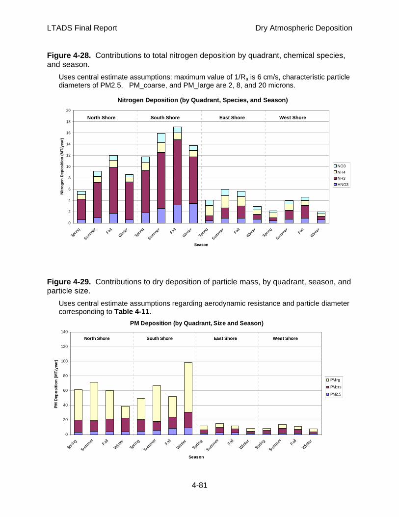
LTADS Final Report Dry Atmospheric Deposition
4-81
Figure 4-28. Contributions to total nitrogen deposition by quadrant, chemical species, and season.
Uses central estimate assumptions: maximum value of 1/Ra is 6 cm/s, characteristic particle diameters of PM2.5, PM_coarse, and PM_large are 2, 8, and 20 microns.
Figure 4-29. Contributions to dry deposition of particle mass, by quadrant, season, and particle size.
Uses central estimate assumptions regarding aerodynamic resistance and particle diameter corresponding to Table 4-11 .
Nitrogen Deposition (by Quadrant, Species, and Seas on)
0
2
4
6
8
10
12
14
16
18
20
Spring
Summer Fall
Wint
er
Spring
Summer Fall
Wint
er
Spring
Summer Fall
Wint
er
Spring
Summer Fall
Wint
er
Season
Nitr
ogen
Dep
ositi
on (
MT
/yea
r)
NO3
NH4
NH3
HNO3
North Shore South Shore East Shore West Shore
PM Deposition (by Quadrant, Size and Season)
0
20
40
60
80
100
120
140
Sprin
g
Summer
Fall
Wint
er
Sprin
g
Summer
Fall
Wint
er
Sprin
g
Summer
Fall
Wint
er
Sprin
g
Summer
Fall
Wint
er
Season
PM
Dep
ositi
on (
MT
/yea
r)
PMlrg
PMcrs
PM2.5
North Shore South Shore East Shore West Shore

LTADS Final Report Dry Atmospheric Deposition
4-82
Figure 4-30. Diurnal variation in relative deposition rates of ammonia and nitric acid gas.
Time series are labeled as paired air quality and meteorological monitoring sites. All values are based upon the central estimate assumptions. Units are (ng-N/ m3)x(cm/s).
Deposition Rate of N as NH3(Annual Average, by Site Pair)
0
200
400
600
800
1000
1200
1400
1600
0 1 2 3 4 5 6 7 8 9 10 11 12 13 14 15 16 17 18 19 20 21 22 23
Hour
N a
s N
H3
(ng-
N/m
³)x(
cm/s
)
TB_CR
BL_SS
LF_USCG
SW_TC
Deposition Rate of N as HNO3(Annual Average by Sites Pairs)
0
100
200
300
400
500
600
700
800
0 1 2 3 4 5 6 7 8 9 10 11 12 13 14 15 16 17 18 19 20 21 22 23
Hour
N a
s H
NO
3 (n
g-N
/m³)
x(cm
/s)
TB_CR
BL_SS
LF_USCG
SW_TC

LTADS Final Report Dry Atmospheric Deposition
4-83
Figure 4-31. Comparison of diurnal variation in estimated mass deposition of PM2.5, PM_coarse, and PM_large for various pairs of air quality and meteorological monitoring sites.
All values are based on the central estimate assumptions. Units are [(ng/m3)x(cm/s)]. Note, vertical scale is expanded for coarse and large fractions compared to fine fraction.
Deposition Rate of Mass (PM2.5)(Annual Average, by Site Pair)
0
200
400
600
800
1000
1200
1400
1600
1800
2000
0 1 2 3 4 5 6 7 8 9 10 11 12 13 14 15 16 17 18 19 20 21 22 23
Hour
Mas
s (n
g/m
³)x(
cm/s
)
TB_CR
BL_SS
LF_USCG
SW_TC

LTADS Final Report Dry Atmospheric Deposition
4-84
Figure 4-31 continued.
Deposition Rate of Mass (PMlrg)(Annual Average, by Site Pair)
0
1000
2000
3000
4000
5000
6000
7000
8000
9000
10000
0 1 2 3 4 5 6 7 8 9 10 11 12 13 14 15 16 17 18 19 20 21 22 23
Hour
Mas
s (n
g/m
³)x(
cm/s
)
TB_CR
BL_SS
LF_USCG
SW_TC
Deposition Rate of Mass (PMcrs)(Annual Average, by Site Pair)
0
1000
2000
3000
4000
5000
6000
7000
8000
9000
10000
0 1 2 3 4 5 6 7 8 9 10 11 12 13 14 15 16 17 18 19 20 21 22 23
Hour
Mas
s (n
g/m
³)x(
cm/s
)
TB_CR
BL_SS
LF_USCG
SW_TC

LTADS Final Report Dry Atmospheric Deposition
4-85
4.8 Summary This chapter has presented the methodology used to calculate seasonal and annual dry deposition to Lake Tahoe, the assumptions used, and ranges of estimated annual dry deposition of nitrogen, phosphorus, and PM mass to the surface of Lake Tahoe. Estimates were based on the ambient concentrations and meteorology observed during LTADS. Due to difficulties in monitoring low concentrations of phosphorus, a representative concentration was assumed to be 40 ng P/m3 for shore and near-shore areas. We assumed a modest decrease of phosphorus and PM (but not nitrogen) concentrations over the Lake for the north and south quadrants. Annual dry deposition of nitrogenous species was estimated to be between 70 and 170 metric tons, with a central estimate of 120 metric tons assuming no decrease in concentrations of nitrogen species on the Lake compared to the monitoring sites. Assuming modest depletion of phosphorus concentrations analogous to those reductions assumed for PM provided estimates for annual dry deposition that ranged from 0.6 to 3 metric tons, with a central estimate of 2.2 metric tons of phosphorus. The estimates of annual PM deposition ranged from 360 to 900 metric tons, with a central estimate of 600 metric tons. An alternative estimate of phosphorus deposition, lower by a factor of two, would be predicted by scaling phosphorus deposition to the estimates for dry deposition of PM using a predicted percent phosphorus in each size fraction of PM. Emission inventory information for the types of sources at Lake Tahoe predicts phosphorus concentrations of 0.07, 0.17, and 0.19 percent in PM2.5, PM_coarse, and PM_large. Using this scaling strategy and the same modest depletion of PM concentrations in the south and north quadrants (as were used for the estimates in Tables 4-10, 4-11, and 4-12 ), results in annual estimates of phosphorus deposition of 0.6 to 1.5 metric tons, with a central estimate of 1 metric ton. This report assumes the values provided in Tables 4-10, 4-11, and 4-12 as the lower bound, central, and upper bound estimates of dry deposition. The next chapter will use a conceptual model, seasonal air quality concentrations from the TWS network and the number of hours when precipitation fell to develop physically reasonable wet deposition estimates. Those estimates of wet deposition will then be combined with the estimates of dry deposition found in Tables 4-10, 4-11, and 4-12 to estimate total atmospheric deposition loads to Lake Tahoe during LTADS.
LTADS Final Report Dry Atmospheric Deposition
4-86
4.9 References Air Resources Board (2005), “Lake Tahoe Atmospheric Deposition Study Interim Report,” ARB Research Division Reports, Cal/EPA 1001 I Street, Sacramento, California 95814. Barthelmie R.J. and S.C. Pryor (2003), “Can satellite sampling of offshore wind speeds realistically represent wind speed distributions?” Journal of Applied Meteorology, 42, 83-94. Brook, J.R., L. Zhang, F. Di-Giovanni, and J. Padro (1999), “Description and evaluation of a model of deposition velocities for routine estimates of air pollutant dry deposition: I Model development,” Atmospheric Environment. 33: 5037-5051. Brook, J.R., L. Zhang, Y.F. Li, and D. Johnson (1999) “Description and evaluation of a model of deposition velocities for routine estimates of air pollutant dry deposition: II Review of past measurements and model results.” Atmospheric Environment. 33: 5053-5070. Brutsaert, W. (1982) "Evaporation into the Atmosphere: Theory, History and Applications " Boston: D. Reidel. (Russian translation: Ispareniye v atmosferu. Leningrad, U.S.S.R.: Gidrometeoizdat. 1985). Byun, D.W. and Dennis (1995), “Design artifacts in Eulerian air quality models: Evaluation of the effects of layer thickness and vertical profile correction on surface ozone concentrations.” Atmospheric Environment, 29, No. 1, 105-126. Charnock, H. (1955), “Wind stress on a water surface,” Quart. J. Roy. Meteor. Soc., 81, 639–640. Garratt, J.R. (1977), “Review of drag coefficients over oceans and continents,” Mon. Weather Rev., 105, 915–929. Giorgi, F. (1986) “A particle dry-deposition parameterization scheme for use in tracer transport models.” J. Geophys. Res., 91, 9794–9806. Giorgi, F. and Chameides, W.L. (2003), Journal of Geophysical Research Atmosphere, 91, 14367+. Hanna, S.R., L.L. Schulman, R.J. Paine, J.E. Pleim, and M. Baer (1985), “Development and evaluation of the offshore and coastal dispersion model” J. Air Poll. Contr. Assoc., 35, 1039-1047. Hicks, B.B. (1982), “Critical assessment document on acid deposition,” ATDL Contrib. File No. 81/24, Atmospheric Turbulence and Diffusion Laboratory, Oak Ridge, TN.

LTADS Final Report Dry Atmospheric Deposition
4-87
Hosker, R.P., Jr., (1974) “A comparison of estimation procedures for over-water plume dispersion.” Presented at the Symposium of Atmospheric Diffusion and Air Pollution, Santa Barbara, California, September 9-13, 1974. Conference Proceedings, 281-288. Larsen, S.E., J.B. Edson, P. Hummelshøj, N.O. Jensen, G. de Leeuw, and P.G. Mestayer (1995), “Dry deposition of particles to ocean surfaces, “ Ophelia, 42, 193–204. Lu R., R.P. Turco, K. Stolzenbach, et al. (2003), “Dry deposition of airborne trace metals on the Los Angeles Basin and adjacent coastal waters,” Journal of Geophysical Research Atmosphere, 108 (D2): 4074-4074. Pleim, J., A. Venkatram and R. Yamartino (1984), “ADOM/TADAP model development program. Volume 4. The dry deposition module,” Ontario Ministry of the Environment, Rexdale, Ontario. Pryor S.C. and Sorensen L.L. (2000), “Nitric acid-sea salt reactions: Implications for nitrogen deposition to water surfaces,” Journal of Applied Meteorology, 39 No. 5, 725-731. Pryor S.C. and Barthelmie R.J. (2003), “Long term variability of flow over the Baltic,” International Journal of Climatology, 23, 271-289. Scire, J.S., F.R. Robe, M.E. Fernau, R.J. Yamartino, (2000), “A User’s Guide for the CALMET Meteorological Model,Version 5,” Earth Tech, Inc., Concord, MA. pp. 332. Scire, J., D.G. Strimaitis, R.J. Yamartino (2000a), ”A User’s Guide for the CALPUFF Dispersion Model (Version 5),“ Earth Tech, Inc., Concord, Massachusetts. pp. 521. Sehmel, G.A., (1980) “Particle and Gas Dry Deposition: A Review” Atmospheric Environment, 14, 983-1011. Seinfeld, J.H., and S.N. Pandis, (1998), “Atmospheric Chemistry and Physics: From Air Pollution to Climate Change”, John Wiley & Sons, Inc., NY. Slinn, S.A. and W.G.N. Slinn (1980), “Predictions for particle deposition and natural waters,“ Atmospheric Environment, 14, 1013-1016. Smith R.I., D. Fowler, M.A. Sutton, C. Flechard, and M. Coyle (2000), “Regional estimation of pollutant gas deposition in the UK: model description, sensitivity analyses and outputs,” Atmospheric Environment, 34, 3757-3777. Stull, R.B. (1988), “An Introduction to Boundary Layer Meteorology”, Kluwer Academic Publishers, Dordrecht, Boston, London. Sun, J. and co-authors (1997), “Lake induced atmospheric circulation (s) during BOREAS,” Journal of Geophysical Research Atmosphere 102, 29, 155-166.

LTADS Final Report Dry Atmospheric Deposition
4-88
Sun JL, D. Vandemark, L. Mahrt, et al. (2001), “Momentum transfer over the coastal zone,” Journal of Geophysical Research Atmosphere, 106 (D12): 12437-12448. Venkatram, A. and J. Pleim (1999), “The electrical analogy does not apply to modeling dry deposition of particles,” Atmospheric Environment, 33, 3075-3076. Valigura, R.A. (1995), “Iterative bulk exchange model for estimating air-water transfer of HNO3” Journal of Geophysical Research Atmosphere, 100, 26045-26050. Wesley M.L. and B.B. Hicks (2000), “A review of the current status of knowledge on dry deposition,” Atmospheric Environment, 34, 2261-2282. Whelpdale, D.M. and R.W. Shaw (1974), Sulfur dioxide removal by turbulent transfer over grass, snow, and water surfaces. Tellus, 26, 1(2), 196-204. Williams, R.M. (1982), “A Model for Dry Deposition of Particles to Natural Water Surfaces,” Atmospheric Environment, 16, No. 8, 1933-1938. Zufall, M.J., C.I. Davidson, P.F. Caffrey, et al. (1998), “Airborne concentrations and dry deposition fluxes of particulate species to surrogate surfaces deployed in Southern Lake Michigan,“ Environmental Science and Technology, 32 (11), 1623-1628.