4 exploration informed search and - uni...

In which we see how information about the state space can prevent algorithms from blundering about in the dark.

:

Chapter 3 showed that uninformed search strategies can find solutions to problems by systematically generating new states and testing them against the goal. Unfortunately, these strategies are incredibly inefficient in most cases. This chapter shows how an informed search strategy-one that uses problem-specific knowledge-can find solutions more efficiently. Section 4.1 describes informed versions of the algorithms in Chapter 3, and Section 4.2 explains how the necessary problem-specific information can be obtained. Sections 4.3 and 4.4 cover algorithms that perform purely local search in the state space, evaluating and modifying one or more current states rather than systematically exploring paths from an initial state. These algorithms are suitable for problems in which the path cost is irrelevant and all that matters is the solution state itself. The family of local-search algorithms includes methods inspired by statistical physics (simulated annealing) and evolutionary biology (genetic algorithms). Finally, Section 4.5 investigates online search, in which the agent is faced with a state space that is completely unknown.

INFORMED SEARCH AND 4 EXPLORATION

INFORMED SEARCH This section shows how an informed search strategy--one that uses problem-specific knowledge beyond the definition of the problem itself-can find solutions more efficiently than an uninformed strategy.

BEST-FIRST SEARCH The general approach we will consider is called best-first search. Best-first search is an instance of the general TREE-SEARCH or GRAPH-SEARCH algorithm in which a node is

EVALUATION FUNCTION selected for expansion based on an evaluation function, f (n) . Traditionally, the node with

the lowest evaluation is selected for expansion, because the evaluation measures distance to the goal. Best-first search can be implemented within our general search framework via a priority queue, a data structure that will maintain the fringe in ascending order of f -values.

The name "best-first search7' is a venerable but inaccurate one. After all, if we could really expand the best node first, it would not be a search at all; it would be a straight march to

Section 4.1. Informed (Heuristic) Search Strategies 95

the goal. All we can do is choose the node that appears to be best according to the evaluation function. If the evaluation function is exactly accurate, then this will indeed ble the best node; in reality, the evaluation function will sometimes be off, and can lead the search astray. Nevertheless, we will stick with the name "best-first search," because "seemingly-best-first search" is a little awkward.

There is a whole family of BEST-FIRST-SEARCH algorithms with different evaluation HEURISTIC FUNCTION functions.' A key component of these algorithms is a heuristic f ~ n c t i o n , ~ denoted h(n):

h(n) = estimated cost of the cheapest path from node n to a goal node.

For example, in Romania, one might estimate the cost of the cheapest path from Arad to Bucharest via the straight-line distance from Arad to Bucharest.

Heuristic functions are the most common form in which additional knowledge of the problem is imparted to the search algorithm. We will study heuristics in more depth in Sec- tion 4.2. For now, we will consider them to be arbitrary problem-specific functions, with one constraint: if n is a goal node, then h(n) = 0. The remainder of this section covers two ways to use heuristic information to guide search.

Greedy best-first search

Greedy best-first search3 tries to expand the node that is closest to the goal, on the: grounds SEARCH

that this is likely to lead to a solution quickly. Thus, it evaluates nodes by using just the heuristic function: f ( n ) = h(n).

Let us see how this works for route-finding problems in Romania, using the straight- line distance heuristic, which we will call hsLD. If the goal is Bucharest, we will need to DlSTANCli

know the straight-line distances to Bucharest, which are shown in Figure 4.1. For example, hsLD(In(Arad)) = 366. Notice that the values of hsLD cannot be computed from the problem description itself. Moreover, it takes a certain amount of experience to know that hSLD is correlated with actual road distances and is, therefore, a useful heuristic.

Arad 366 Mehadia 24 1 Bucharest 0 Neamt 234 Craiova 160 Oradea 380 Drobeta 242 Pitesti 100 Eforie 161 Rimnicu Vilcea 193 Fagaras 176 Sibiu 253 Giurgiu 77 Timisoara 329 Hirsova 151 Urziceni 80 Iasi 226 Vaslui 199 Lugoj 244 Zerind 374

Figure 4.1 Values of ~SLD-straight-line distances to B u c h a r e s t .

Exercise 4.3 asks you to show that this family includes several familiar uninformed algorithms. "heuristic function h(n) takes a node as input, but it depends only on the state at that node.

Our first edition called this greedy search; other authors have called it best-first search. Our mare general usage of the latter tern follows Pearl (1984).

96 Chapter 4. Informed Search and Exploration

(a) The initial state

(c) After expanding Sibiu

d& <&$&

(d) After expanding Fagaras

253 0

Figure 4.2 Stages in a greedy best-first search for Bucharest using the straight-line distance heuristic hsto. Nodes are labeled with their h-values.

Figure 4.2 shows the progress of a greedy best-first search using hsLD to find a path from Arad to Bucharest. The first node to be expanded from Arad will be Sibiu, because it is closer to Bucharest than either Zerind or Timisoara. The next node to be expanded will be Fagaras, because it is closest. Fagaras in turn generates Bucharest, which is the goal. For this particular problem, greedy best-first search using hsLD finds a solution without ever expanding a node that is not on the solution path; hence, its search cost is minimal. It is not optimal, however: the path via Sibiu and Fagaras to Bucharest is 32 kilometers longer than the path through Rimnicu Vilcea and Pitesti. This shows why the algorithm is called "greedy2'-at each step it tries to get as close to the goal as it can.

Minimizing h(n) is susceptible to false starts. Consider the problem of getting from Iasi to Fagaras. The heuristic suggests that Neamt be expanded first, because it is closest


to Fagaras, but it is a dead end. The solution is to go first to Vaslui-a step that is actually farther from the goal according to the heuristic-and then to continue to Urziceni, Bucharest, and Fagaras. In this case, then, the heuristic causes unnecessary nodes to be expanded. Fur- thermore, if we are not careful to detect repeated states, the solution will never be found-the search will oscillate between Neamt and Iasi.

Greedy best-first search resembles depth-first search in the way it prefers to follow a single path all the way to the goal, but will back up when it hits a dead end. It suffers from the same defects as depth-first search-it is not optimal, and it is incomplete (becixuse it can start down an infinite path and never return to try other possibilities). The worst-case time and space complexity is O(bm), where m is the maximum depth of the search space. With a good heuristic function, however, the complexity can be reduced substantially. Tlie amount of the reduction depends on the particular problem and on the quality of the heuristic.

A* search: Minimizing the total estimated solution cost

A* SEARCH The most widely-known form of best-first search is called A* search (pronounced "A-star search"). It evaluates nodes by combining g(n), the cost to reach the node, and h(n.), the cost to get from the node to the goal:

Since g(n) gives the path cost from the start node to node n , and h(n) is the estirnated cost of the cheapest path from n to the goal, we have

f (n) = estimated cost of the cheapest solution through n

Thus, if we are trying to find the cheapest solution, a reasonable thing to try first is the node with the lowest value of g(n) + h(n) . It turns out that this strategy is more than just reasonable: provided that the heuristic function h(n) satisfies certain conditions, K search is both complete and optimal.

The optimality of A* is straightforward to analyze if it is used with TREE-SEARCH. ADMISSIBLE HEURISTIC In this case, A* is optimal if h(n) is an admissible heuristic-that is, provided that h(n)

never overestimates the cost to reach the goal. Admissible heuristics are by nature optimistic, because they think the cost of solving the problem is less than it actually is. Since g(n) is the exact cost to reach n, we have as immediate consequence that f ( n ) never overestimates the true cost of a solution through n.

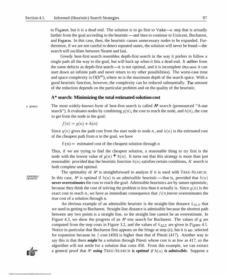
An obvious example of an admissible heuristic is the straight-line distance hsLD that we used in getting to Bucharest. Straight-line distance is admissible because the shortest path between any two points is a straight line, so the straight line cannot be an overestimate. In Figure 4.3, we show the progress of an A* tree search for Bucharest. The values of g are computed from the step costs in Figure 3.2, and the values of hsLD are given in Figure 4.1. Notice in particular that Bucharest first appears on the fringe at step (e), but it is noit selected for expansion because its f -cost (450) is higher than that of Pitesti (417). Another way to say this is that there might be a solution through Pitesti whose cost is as low as 417, so the algorithm will not settle for a solution that costs 450. From this example, we can extract a general proof that A* using TREE-SEARCH is optimal if h(n) is admissible. Suppose a


(a) The initial state 366=0+366

(b) After expanding Arad

393=140+253

(c) After expanding Sibiu

646=280+366 415=239+176 671=291+380 413=220+193

(d) After expanding Rimnicu Vilce

526=366+160 417=317+100 553=300+253

(e) After expanding Fagaras

591=338+253 450=450+0 526=366+160 417=317+100 553=300+253

(f) After expanding Pitesti

418=418+0 615=455+160 607=414+193

Figure 4.3 Stages in an A* search for Bucharest. Nodes are labeled with f = g + h. The h values are the straight-line distances to Bucharest taken from Figure 4.1.


suboptimal goal node G2 appears on the fringe, and let the cost of the optimal soluti~on be C*. Then, because G2 is suboptimal and because h(G2) = 0 (true for any goal node), vie know

f (G2) = g(G2) + h(G2) = g(G2) > C* . Now consider a fringe node n that is on an optimal solution path-for example, Pitesti in the example of the preceding paragraph. (There must always be such a node if a solution exists.) If h(n) does not overestimate the cost of completing the solution path, then we know that

f (n) = g(n) + h(n) 5 C* . Now we have shown that f (n) 5 C* < f (G2), so G2 will not be expanded anti A* must return an optimal solution.

If we use the GRAPH-SEARCH algorithm of Figure 3.19 instead of TREE-SEARCH, then this proof breaks down. Suboptimal solutions can be returned because GRAPH-SEARCH

can discard the optimal path to a repeated state if it is not the first one generated. (See Exercise 4.4.) There are two ways to fix this problem. The first solution is to extend GRAPH-SEARCH so that it discards the more expensive of any two paths found to the same node. (See the discussion in Section 3.5.) The extra bookkeeping is messy, but it does guarantee optimality. The second solution is to ensure that the optimal path to any repeated state is always the first one followed-as is the case with uniform-cost search. This property holds if

CONSISTENCY we impose an extra requirement on h(n), namely the requirement of consistency (also called MONOTONICIN monotonicity). A heuristic h(n) is consistent if, for every node n and every successor n' of

n generated by any action a, the estimated cost of reaching the goal from n is no greater than the step cost of getting to n' plus the estimated cost of reaching the goal from n':

h(n) 5 c(n, a, n') t h(nf) . TRlANGLli INEQUALIN This is a form of the general triangle inequality, which stipulates that each side of ;I triangle

cannot be longer than the sum of the other two sides. Here, the triangle is formed by n, n', and the goal closest to n. It is fairly easy to show (Exercise 4.7) that every consistent heuristic is also admissible. The most important consequence of consistency is the following: A* using GRAPH-SEARCH is optimal $h(n) is consistent.

Although consistency is a stricter requirement than admissibility, one has to wlork quite hard to concoct heuristics that are admissible but not consistent. All the admissible heuristics we discuss in this chapter are also consistent. Consider, for example, hsLD. We know that Ithe general triangle inequality is satisfied when each side is measured by the straight-line distance, and that the straight-line distance between n and n' is no greater than c(n, a, n'). IHence, hsLD is a consistent heuristic.

Another important consequence of consistency is the following: Zf h(n) is consistent, then the values off (n) along any path are nondecueasing. The proof follows directly from the definition of consistency. Suppose n' is a successor of n; then g(n') = g(n) + c(n, a , n') for some a, and we have

f ( n f ) = g(nf) + h(nf) = g(n) + c(n, a , n') + h(nf) 2 g(n) + h(n) = f (n) . It follows that the sequence of nodes expanded by A* using GRAPH-SEARCH is in nondecreasing order of f (n). Hence, the first goal node selected for expansion must be an optimal solution, since all later nodes will be at least as expensive.


Figure 4.4 Map of Romania showing contours at f = 380, f = 400 and f = 420, with Arad as the start state. Nodes inside a given contour have f -costs less than or equal to the contour value.

The fact that f -costs are nondecreasing along any path also means that we can draw CONTOURS contours in the state space, just like the contours in a topographic map. Figure 4.4 shows an

example. Inside the contour labeled 400, all nodes have f (n) less than or equal to 400, and so on. Then, because A* expands the fringe node of lowest f -cost, we can see that an A* search fans out from the start node, adding nodes in concentric bands of increasing f -cost.

With uniform-cost search (A* search using h(n) = O), the bands will be "circular" around the start state. With more accurate heuristics, the bands will stretch toward the goal state and become more narrowly focused around the optimal path. If C* is the cost of the optimal solution path, then we can say the following:

A* expands all nodes with f (n) < C*. A* might then expand some of the nodes right on the "goal contour" (where f (n) = C*) before selecting a goal node.

Intuitively, it is obvious that the first solution found must be an optimal one, because goal nodes in all subsequent contours will have higher f -cost, and thus higher g-cost (because all goal nodes have h(n) = 0). Intuitively, it is also obvious that A* search is complete. As we add bands of increasing f , we must eventually reach a band where f is equal to the cost of the path to a goal state.4

Notice that A* expands no nodes with f (n) > C*-for example, Timisoara is not expanded in Figure 4.3 even though it is a child of the root. We say that the subtree below

PRUNING Timisoara is pruned; because hsLD is admissible, the algorithm can safely ignore this subtree

* Completeness requires that there be only finitely many nodes with cost less than or equal to C*, a condition that is true if all step costs exceed some finite t and if b is finite.


while still guaranteeing optimality. The concept of pruning-eliminating possibilities from consideration without having to examine them-is important for many areas of AI.

One final observation is that among optimal algorithms of this type-algorithms that extend search paths from the root-A* is optimally efficient for any given heuristic function. That is, no other optimal algorithm is guaranteed to expand fewer nodes than A* (except possibly through tie-breaking among nodes with f (n) = C*). This is because any algorithm that does not expand all nodes with f (n) < C* runs the risk of missing the optimal solution.

That A* search is complete, optimal, and optimally efficient among all such algorithms is rather satisfying. Unfortunately, it does not mean that A* is the answer to all our searching needs. The catch is that, for most problems, the number of nodes within the goal contour search space is still exponential in the length of the solution. Although the proof of the result is beyond the scope of this book, it has been shown that exponential growth will occur unless the error in the heuristic function grows no faster than the logarithm of the actual path cost. In mathematical notation, the condition for subexponential growth is that

where h* (n) is the true cost of getting from n to the goal. For almost all heuristics in practical use, the error is at least proportional to the path cost, and the resulting exponential growth eventually overtakes any computer. For this reason, it is often impractical to insist on finding an optimal solution. One can use variants of A* that find suboptimal solutions quickly, or one can sometimes design heuristics that are more accurate, but not strictly admissible. In any case, the use of a good heuristic still provides enormolus savings compared to the use of an uninformed search. In Section 4.2, we will look at the question of designing good heuristics.

Computation time is not, however, A*'s main drawback. Because it keeps all generated nodes in memory (as do all GRAPH-SEARCH algorithms), A* usually runs out of space long before it runs out of time. For this reason, A* is not practical for many large-scale problems. Recently developed algorithms have overcome the space problem without sacrificing optimality or completeness, at a small cost in execution time. These are discussed next.

Memory-bounded heuristic search

The simples1 way to reduce memory requirements for A" is to adapt the idea of iterative deepening to the heuristic search context, resulting in the iterative-deepening A" (IDA*) algorithm. The main difference between IDA* and standard iterative deepening is that the cutoff used is the f -cost (g + h) rather than the depth; at each iteration, the cutoff value is the smallest f -cost of any node that exceeded the cutoff on the previous iteration. IDA* is practical for many problems with unit step costs and avoids the substantial overhead associated with keeping a sorted queue of nodes. Unfortunately, it suffers from the same difficulties with real- valued costs as does the iterative version of uniform-cost search described in Exercise 3.11. This section briefly examines two more recent memory-bounded algorithms, called RBFS and MA*.

RECURSIVE BEST-FIRST SEARCH Recursive best-first search (RBFS) is a simple recursive algorithm that attempts to

mimic the operation of standard best-first search, but using only linear space. The algorithm is shown in Figure 4.5. Its structure is similar to that of a recursive depth-first search, but rather


function RECURSIVE-BE~T-FIR~T-SEARCH(~~O~~~~) returns a solution, or failure RBFS(problem, MAKE-NoDE(INITIAL-STATE[~~O~~~~]), oo)

function RBFS(problem, node, f-limit) returns a solution, or failure and a new f -cost limit if GoAL-TEsT[~~o~~~~](STATE[~O~~]) then return node successors +- E X P A N D ( ~ O ~ ~ , problem) ' if successors is empty then return failure, oo for each s in successors do

f [sl +max(g(s ) + h(s ) , f [nodel) repeat

best +the lowest f -value node in successors i f f [best] > f-limit then return failure, f [best] alternative +- the second-lowest f -value among successors result, f [best] + RBFS(problem, best,min( f-limit, alternative)) if result # failure then return result

Figure 4.5 The algorithm for recursive best-first search. 1 than continuing indefinitely down the current path, it keeps track of the f-value of the best alternative path available from any ancestor of the current node. If the current node exceeds this limit, the recursion unwinds back to the alternative path. As the recursion unwinds, RBFS replaces the f -value of each node along the path with the best f -value of its children. In this way, RBFS remembers the f -value of the best leaf in the forgotten subtree and can therefore decide whether it's worth reexpanding the subtree at some later time. Figure 4.6 shows how RBFS reaches Bucharest.

RBFS is somewhat more efficient than IDA*, but still suffers from excessive node regeneration. In the example in Figure 4.6, RBFS first follows the path via Rimnicu Vilcea, then "changes its mind" and tries Fagaras, and then changes its mind back again. These mind changes occur because every time the current best path is extended, there is a good chance that its f -value will increase-h is usually less optimistic for nodes closer to the goal. When this happens, particularly in large search spaces, the second-best path might become the best path, so the search has to backtrack to follow it. Each mind change corresponds to an iteration of IDA*, and could require many reexpansions of forgotten nodes to recreate the best path and extend it one more node.

Like A*, RBFS is an optimal algorithm if the heuristic function h(n) is admissible. Its space complexity is linear in the depth of the deepest optimal solution, but its time complexity is rather difficult to characterize: it depends both on the accuracy of the heuristic function and on how often the best path changes as nodes are expanded. Both IDA* and RBFS are subject to the potentially exponential increase in complexity associated with searching on graphs (see Section 3.5), because they cannot check for repeated states other than those on the current path. Thus, they may explore the same state many times.

IDA* and RBFS suffer from using too little memory. Between iterations, IDA* retains only a single number: the current f -cost limit. RBFS retains more information in memory,


MA'

SMA'

(a) After expanding Arad, Sibiu, and Rimnicu Vilcea

(a) After expandi and Rimnicu Vilcea

(b) After unwinding back to Sibiu and expanding Fagaras

(c) After switching back to Rimnicu Vilcea and expanding Pitesti

9

(c) After switching back to Rimnicu Vilcea and expanding Pitesti

Figure 4.6 Stages in an RBFS search for the shortest route to Bucharest. The f-limit value for each recursive call is shown on top of each current node. (a) The path via Rimnicu Vilcea is followed until the current best leaf (Pitesti) has a value that is worse than the best alternative path (Fagaras). (b) The recursion unwinds and the best leaf value of the forgotten subtree (417) is backed up to Rimnicu Vilcea; then Fagaras is expanded, revealing a best leaf value of 450. (c) The recursion unwinds and the best leaf value of the forgotten subtree (450) is backed up to Fagaras; then Rirnnicu Vilcea is expanded. This time, because the best alternative path (through Timisoara) costs at least 447, the expansion continues to Bucharest.

J

but it uses only linear space: even if more memory were available, RBFS has no way to make use of it.

It seems sensible, therefore, to use all available memory. Two algorithms that do this are MA* (memory-bounded A*) and SMA* (simplified MA*). We will describe SMA*, which

1 04 Chapter 4. Informed Search and Exploration

is-well-simpler. SMA* proceeds just like A*, expanding the best leaf until memory is full. At this point, it cannot add a new node to the search tree without dropping an old one. SMA* always drops the worst leaf node-the one with the highest f-value. Like RBFS, SMA* then backs up the value of the forgotten node to its parent. In this way, the ancestor of a forgotten subtree knows the quality of the best path in that subtree. With this information, SMA* regenerates the subtree only when all otherpaths have been shown to look worse than the path it has forgotten. Another way of saying this is that, if all the descendants of a node n are forgotten, then we will not know which way to go from n, but we will still have an idea of how worthwhile it is to go anywhere from n.

The complete algorithm is too complicated to reproduce here,5 but there is one subtlety worth mentioning. We said that SMA* expands the best leaf and deletes the worst leaf. What if all the leaf nodes have the same f -value? Then the algorithm might select the same node for deletion and expansion. SMA* solves this problem by expanding the newest best leaf and deleting the oldest worst leaf. These can be the same node only if there is only one leaf; in that case, the current search tree must be a single path from root to leaf that fills all of memory. If the leaf is not a goal node, then even if it is on an optimal solution path, that solution is not reachable with the available memory. Therefore, the node can be discarded exactly as if it had no successors.

SMA* is complete if there is any reachable solution-that is, if d, the depth of the shallowest goal node, is less than the memory size (expressed in nodes). It is optimal if any optimal solution is reachable; otherwise it returns the best reachable solution. In practical terms, SMA* might well be the best general-purpose algorithm for finding optimal solutions, particularly when the state space is a graph, step costs are not uniform, and node generation is expensive compared to the additional overhead of maintaining the open and closed lists.

On very hard problems, however, it will often be the case that SMA* is forced to switch back and forth continually between a set of candidate solution paths, only a small subset of

THRASHING which can fit in memory. (This resembles the problem of thrashing in disk paging systems.) Then the extra time required for repeated regeneration of the same nodes means that problems that would be practically solvable by A*, given unlimited memory, become intractable for SMA*. That is to say, memory limitations can make a problem intractable from the point of view of computation time. Although there is no theory to explain the tradeoff between time and memory, it seems that this is an inescapable problem. The only way out is to drop the optimality requirement.

Learning to search better

We have presented several fixed strategies-breadth-first, greedy best-first, and so on-that have been designed by computer scientists. Could an agent learn how to search better? The answer is yes, and the method rests on an important concept called the metalevel state space. SPACE

Each state in a metalevel state space captures the internal (computational) state of a program STATE that is searching in an object-level state space such as Romania. For example, the internal SPACE

state of the A* algorithm consists of the current search tree. Each action in the metalevel state

A rough sketch appeared in the first edition of this book.

Section 4.2. Heuristic Functions 105

space is a computation step that alters the internal state; for example, each computation step in A* expands a leaf node and adds its successors to the tree. Thus, Figure 4.3, which shows a sequence of larger and larger search trees, can be seten as depicting a path in the metalevel state space where each state on the path is an object-level search tree.

Now, the path in Figure 4.3 has five steps, including one step, the expansion of Fagaras, that is not especially helpful. For harder problems, th~ere will be many such missteps, and a metalevel learning algorithm can learn from these experiences to avoid exploring unpromis- ing subtrees. The techniques used for this kind of learning are described in Chapter 21. The goal of leaning is to minimize the total cost of problem solving, trading off computational expense and path cost.

In this section, we will look at heuristics for the 8-puzzle, in order to shed light on the nature of heuristics in general.

The 8-puzzle was one of the earliest heuristic search problems. As mentioned in Sec- tion 3.2, the object of the puzzle is to slide the tiles horizontally or vertically into the empty space until the configuration matches the goal configuration (Figure 4.7).

Start State Goal State

Figure 4.7 A typical instance of the 8-puzzle. The s~olution p- is 26 steps long.

The average solution cost for a randomly generated %-puzzle instance is about 22 steps. The branching factor is about 3. (When the empty tile is in the middle, there are four possible moves; when it is in a corner there are two; and when it is along an edge there are three.) This means that an exhaustive search to depth 22 would look at about 322 = 3.1 x lo1' states. By keeping track of repeated states, we could cut this down by a factor of about 170,000, because there are only 9!/2 = 181,440 distinct states that are reachable. (See Exercise 3.4.) This is a manageable number, but the corresponding number for the 15-puzzle is roughly 1013, so the next order of business is to find a good heuristic function. If we want to find the shortest solutions by using #, we need a heuristic function that never overestimates the number of steps to the goal. There is a long history of such heuristics for the 15-puzzle; here are two commonly-used candidates:


MANHATTAN DISTANCE

hl = the number of misplaced tiles. For Figure 4.7, all of the eight tiles are out of position, so the start state would have hl = 8. hl is an admissible heuristic, because it is clear that any tile that is out of place must be moved at least once.

h2 = the sum of the distances of the tiles from their goal positions. Because tiles cannot move along diagonals, the distance we will count is the sum of the horizontal and vertical distances. This is sometimes called the city block distance or Manhattan distance. h2 is also admissible, because all any move can do is move one tile one step closer to the goal. Tiles 1 to 8 in the start state give a Manhattan distance of

h 2 = 3 + l + 2 + 2 + 2 + 3 + 3 + 2 = 1 8 .

As we would hope, neither of these overestimates the true solution cost, which is 26.

The effect of heuristic accuracy on performance EFFECTIVE FACTOR One way to characterize the quality of a heuristic is the effective branching factor b*. If the

total number of nodes generated by A* for a particular problem is N, and the solution depth is d, then b* is the branching factor that a uniform tree of depth d would have to have in order to contain N + 1 nodes. Thus,

N + 1 = 1 + b* + (b*)2 + . . . + ( b * ) d .

For example, if A* finds a solution at depth 5 using 52 nodes, then the effective branching factor is 1.92. The effective branching factor can vary across problem instances, but usually it is fairly constant for sufficiently hard problems. Therefore, experimental measurements of b* on a small set of problems can provide a good guide to the heuristic's overall usefulness. A well-designed heuristic would have a value of b* close to 1, allowing fairly large problems to be solved.

To test the heuristic functions hl and ha, we generated 1200 random problems with solution lengths from 2 to 24 (100 for each even number) and solved them with iterative deepening search and with A* tree search using both hl and h2. Figure 4.8 gives the average number of nodes generated by each strategy and the effective branching factor. The results suggest that h2 is better than hl, and is far better than using iterative deepening search. On our solutions with length 14, A* with hz is 30,000 times more efficient than uninformed iterative deepening search.

One might ask whether h2 is always better than hl. The answer is yes. It is easy to see from the definitions of the two heuristics that, for any node n, h2(n) 2 hl (n). We thus say

DOMINATION that hZ dominates hl. Domination translates directly into efficiency: A* using h2 will never expand more nodes than A* using hl (except possibly for some nodes with f (n) = C*). The argument is simple. Recall the observation on page 100 that every node with f (n) < C* will surely be expanded. This is the same as saying that every node with h(n) < C* - g(n) will surely be expanded. But because ha is at least as big as hl for all nodes, every node that is surely expanded by A* search with ha will also surely be expanded with hl, and hl might also cause other nodes to be expanded as well. Hence, it is always better to use a heuristic function with higher values, provided it does not overestimate and that the computation time for the heuristic is not too large.


Inventing admissible heuristic functions

d

2 4 6 8

10 12 14

We have seen that both hl (misplaced tiles) and 1~~ (Manhattan distance) are fairly good heuristics for the 8-puzzle and that hz is better. How might one have come up with h2? Is it possible for a computer to invent such a heuristic mechanically?

hl and hz are estimates of the remaining path length[ for the 8-puzzle, but they are also perfectly accurate path lengths for simpl.$ed versions of the puzzle. If the rules of the puzzle were changed so that a tile could move anywhere, instead of just to the adjacent empty square, then hl would give the exact number of steps in the shortest solution. Similarly, if a tile could move one square in any direction, even onto an occupied square, then h2 would give the exact number of steps in the shortest solution. A pro~blem with fewer restrictions on

RELAXED PROBLEM the actions is called a relaxed problem. The cost of an optimal solution to a relaxedproblem is an admissible heuristic for the original problem. The heuristic is admissible because the optimal solution in the original problem is, by defj~nition, also a solution in the relaxed problem and therefore must be at least as expensive as the optimal solution in the relaxed problem. Because the derived heuristic is an exact cost for the relaxed problem, it must obey the triangle inequality and is therefore consistent (see page 99).

If a problem definition is written down in a formal1 language, it is possible to construct relaxed problems a~tornat ical l~ .~ For example, if the 8-puzzle actions are described as

A tile can move from square A to square B if A is horizontally or vertically adjacent to B an(d B is blank,

In Chapters 8 and 11, we will describe formal languages suitable for this task; with formal descriptions that can be manipulated, the construction of relaxed problems can be automated. For now, we will use English.

Search Cost

1 ;;:: 1 ;:: 1 ,I - 7276 676 18094 1219 -

- 39135 1641 -

IDS

10 112 680

6384 47127

3644035 -

Effective Branching Factor

Figure 4.8 Comparison of the search costs and effective branching factors for the ITERATI VE-DEEPENING-SEARCH and A* algorithms ,with hl , h2. Data are averaged over 100 instances of the &puzzle, for various solution lengths.

IDS

2.45 2.87 ;!.73 2.80 2+.79 2.78 -

1.45 1.46 1.47 1.48 1.48

A*(hl)

6 13 20 39 93

227 539

1.25 1.26 1.27 1.28 1.26

A*(h2)

6 12 18 25 39 73

113

A*(hl)

1.79 1.48 1.34 1.33 1.38 1.42 1.44

A*(ha)

1.79 1.45 1.30 1.24 1.22 1.24 1.23


we can generate three relaxed problems by removing one or both of the conditions:

(a) A tile can move from square A to square B if A is adjacent to B. (b) A tile can move from square A to square B if B is blank. (c) A tile can move from square A to square B.

From (a), we can derive hz (Manhattan distance). The reasoning is that h2 would be the proper score if we moved each tile in turn to its destination. The heuristic derived from (b) is discussed in Exercise 4.9. From (c), we can derive hl (misplaced tiles), because it would be the proper score if tiles could move to their intended destination in one step. Notice that it is crucial that the relaxed problems generated by this technique can be solved essentially without search, because the relaxed rules allow the problem to be decomposed into eight independent subproblems. If the relaxed problem is hard to solve, then the values of the corresponding heuristic will be expensive to ~ b t a i n . ~

A program called ABSOLVER can generate heuristics automatically from problem definitions, using the "relaxed problem" method and various other techniques (Prieditis, 1993). ABSOLVER generated a new heuristic for the 8-puzzle better than any preexisting heuristic and found the first useful heuristic for the famous Rubik's cube puzzle.

One problem with generating new heuristic functions is that one often fails to get one "clearly best" heuristic. If a collection of admissible heuristics hl . . . h, is available for a problem, and none of them dominates any of the others, which should we choose? As it turns out, we need not make a choice. We can have the best of all worlds, by defining

h(n) = max{hl (n), . . . , h,(n) ) .

This composite heuristic uses whichever function is most accurate on the node in question. Because the component heuristics are admissible, h is admissible; it is also easy to prove that h is consistent. Furthermore, h dominates all of its component heuristics.

SUBPROBLEM Admissible heuristics can also be derived from the solution cost of a subproblem of a given problem. For example, Figure 4.9 shows a subproblem of the 8-puzzle instance in Figure 4.7. The subproblem involves getting tiles 1, 2, 3, 4 into their correct positions. Clearly, the cost of the optimal solution of this subproblem is a lower bound on the cost of the complete problem. It turns out to be substantially more accurate than Manhattan distance in some cases.

PAUERN DATABASES The idea behind pattern databases is to store these exact solution costs for every possible subproblem instance-in our example, every possible configuration of the four tiles and the blank. (Notice that the locations of the other four tiles are irrelevant for the purposes of solving the subproblem, but moves of those tiles do count towards the cost.) Then, we compute an admissible heuristic hDB for each complete state encountered during a search simply by looking up the corresponding subproblem configuration in the database. The database itself is constructed by searching backwards froin the goal state and recording the cost of each new pattern encountered; the expense of this search is amortized over many subsequent problem instances.

Note that a perfect heuristic can be obtained simply by allowing h to run a full breadth-first search "on the sly." Thus, there is a tradeoff between accuracy and computation time for heuristic functions.


Start State Goal State

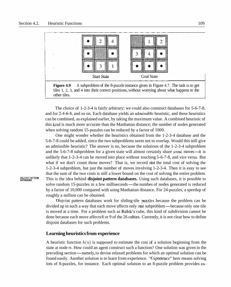
Figure 4.9 A subproblem of the 8-puzzle instance given in Figure 4.7. The task is to get tiles 1, 2, 3, and 4 into their correct positions, without worrying about what happens to the other tiles.

The choice of 1-2-3-4 is fairly arbitrary; we could also construct databases for 5-6-7-8, and for 2-4-64, and so on. Each database yields an admissible heuristic, and these heuristics can be combined, as explained earlier, by taking the maximum value. A combined heuristic of this lund is much more accurate than the Manhattan distance; the number of nodes generated when solving random 15-puzzles can be reduced by a factor of 1000.

One might wonder whether the heuristics obtained from the 1-2-3-4 database and the 5-6-7-8 could be added, since the two subproblems seem not to overlap. Would this still give an admissible heuristic? The answer is no, because the solutions of the 1-2-3-4 subproblem and the 5-6-7-8 subproblem for a given state will almost certainly share some moves-it is unlikely that 1-2-3-4 can be moved into place without touching 5-6-7-8, and vice versa. But what if we don't count those moves? That is, we record niot the total cost of solving the 1-2-3-4 subproblem, but just the number of moves involving 1-2-3-4. Then it is easy to see that the sum of the two costs is still a lower bound on the cost of solving the entire problem. This is the idea behind disjoint pattern databases. Using such databases, it is possible to DATABASES

solve random 15-puzzles in a few milliseconds-the numbes of nodes generated is reduced by a factor of 10,000 compared with using Manhattan distance. For 24-puzzles, a speedup of roughly a million can be obtained.

Disjoint pattern databases work for sliding-tile ]puzzles because the problem can be divided up in such a way that each move affects only onie subproblem-because only one tile is moved at a time. For a problem such as Rubik's cube, this kind of subdivision cannot be done because each move affects 8 or 9 of the 26 cubies. Currently, it is not clear how to define disjoint databases for such problems.

Learning heuristics from experience

A heuristic function h(n) is supposed to estimate the cost of a solution beginning from the state at node n. How could an agent construct such a function? One solution was given in the preceding section-namely, to devise relaxed problems for which an optimal solution can be found easily. Another solution is to learn from experience. "E.xperience" here means solving lots of 8-puzzles, for instance. Each optimal solution to an 8-puzzle problem provides ex-


amples from which h(n) can be learned. Each example consists of a state from the solution path and the actual cost of the solution from that point. From these examples, an inductive learning algorithm can be used to construct a function h(n) that can (with luck) predict solution costs for other states that arise during search. Techniques for doing just this using neural nets, decision trees, and other methods are demonstrated in Chapter 18. (The reinforcement learning methods described in Chapter 21 are also applicable.)

FEATURES Inductive learning methods work best when supplied with features of a state that are relevant to its evaluation, rather than with just the raw state description. For example, the feature "number of misplaced tiles" might be helpful in predicting the actual distance of a state from the goal. Let's call this feature XI (n). We could take 100 randomly generated 8-puzzle configurations and gather statistics on their actual solution costs. We might find that when XI (n) is 5, the average solution cost is around 14, and so on. Given these data, the value of XI can be used to predict h(n). Of course, we can use several features. A second feature xz(n) might be "number of pairs of adjacent tiles that are also adjacent in the goal state." How should XI (n) and xa(n) be combined to predict h(n)? A common approach is to use a linear combination:

h(n) = clx~(n) + c2x~(n) .

The constants cl and ca are adjusted to give the best fit to the actual data on solution costs. Presumably, cl should be positive and c2 should be negative.

4.3 LOCAL SEARCH ALGORITHMS AND OPTIMIZATION PROBLEMS

The search algorithms that we have seen so far are designed to explore search spaces systematically. This systematicity is achieved by keeping one or more paths in memory and by recording which alternatives have been explored at each point along the path and which have not. When a goal is found, the path to that goal also constitutes a solution to the problem.

In many problems, however, the path to the goal is irrelevant. For example, in the 8- queens problem (see page 66), what matters is the final configuration of queens, not the order in which they are added. This class of problems includes many important applications such as integrated-circuit design, factory-floor layout, job-shop scheduling, automatic programming, telecommunications network optimization, vehicle routing, and portfolio management.

If the path to the goal does not matter, we might consider a different class of algo- LOCALSEARCH rithms, ones that do not worry about paths at all. Local search algorithms operate using CURRENTSTATE a single current state (rather than multiple paths) and generally move only to neighbors

of that state. Typically, the paths followed by the search are not retained. Although local search algorithms are not systematic, they have two key advantages: (1) they use very little memory-usually a constant amount; and (2) they can often find reasonable solutions in large or infinite (continuous) state spaces for which systematic algorithms are unsuitable.

In addition to finding goals, local search algorithms are useful for solving pure op- OPTIMIZATION PROBLEMS timization problems, in which the aim is to find the best state according to an objective OBJECTIVE FUNCTION function. Many optimization problems do not fit the "standard" search mode1 introduced in

Section 4.3. Local Search Algorithms and Optimization Problems 111

Chapter 3. For example, nature provides an objectiv~e function-reproductive fitness-that Darwinian evolution could be seen as attempting to optimize, but there is no "goal test" and no "path cost" for this problem.

To understand local search, we will find it very useful to consider the state space land- STATE SPACE LANDSCAPE scape (as in Figure 4.10). A landscape has both "localtion" (defined by the state) and "eleva-

tion" (defined by the value of the heuristic cost function or objective function). If elevation GLOBALMINIMUM corresponds to cost, then the aim is to find the lowest valley-a global minimum; if eleva-

tion corresponds to an objective function, then the aim is to find the highest peak-a global GLOBALMAXIMUM maximum,. (You can convert from one to the other just by inserting a minus sign.) Local

search algorithms explore this landscape. A complete, local search algorithm always finds a goal if one exists; an optimal algorithm always finds a, global minimum/maximum.

maximum

I I b state space current

state

Figure 4.10 A one-dimensional state space landscape in which elevation corresponds to the objective function. The aim is to find the global maximum. Hill-climbing search modifies

I the current state to try to improve it, as shown by the an-ow. The various topographic features are defined in the text.

Hill-climbing search

HILL-CLIMBING The hill-climbing search algorithm is shown in Figure 4.1 1. It is simply a loop that continually moves in the direction of increasing value-that is, uphill. It terminates when it reaches a "peak" where no neighbor has a higher value. The algorithm does not maintain a search tree, so the current node data structure need only record the state and its objective function value. Hill-climbing does not look ahead beyond the immediate neighbors of the current state. This resembles trying to find the top of Mount Everest in a thick fog while suffering from amnesia.

To illustrate hill-climbing, we will use the 8-queens problem introduced on page 66. Local-search algorithms typically use a complete-state formulation, where each state has 8 queens on the board, one per column. The successor function returns all possible states generated by moving a single queen to another square in the same column (so each state has


function H I L L - C L I M B I N G ( ~ ~ ~ ~ ~ ~ ~ ) returns a state that is a local maximum inputs: problem, a problem local variables: current, a node

neighbor, a node

current +- MAKE-NODE(INITIAL-STATE[~~O~~~~]) loop do

neighbor +- a highest-valued successor of curren.t if VA~uE[neighbor] < VALUE[current] then return S ~ ~ ~ ~ [ c u r r e n t ] current t neighbor

Figure 4.11 The hill-climbing search algorithm (steepest ascent version), which is the most basic local search technique. At each step the current node is replaced by the best neighbor; in this version, that means the neighbor with the highest VALUE, but if a heuristic cost estimate h is used, we would find the neighbor with the lowest h.

(a) (b)

Figure 4.12 (a) An 8-queens state with heuristic cost estimate h = 17, showing the value of h for each possible successor obtained by moving a queen within its column. The best moves are marked. (b) A local minimum in the 8-queens state space; the state has h = 1 but every successor has a higher cost.

8 x 7 = 56 successors). The heuristic cost function h is the number of pairs of queens that are attacking each other, either directly or indirectly. The global minimum of this function is zero, which occurs only at perfect solutions. Figure 4.12(a) shows a state with h = 17. The figure also shows the values of all its successors, with the best successors having h = 12. Hill-climbing algorithms typically choose randomly among the set of best successors, if there is more than one.


GREEDY LOCAL SEARCH Hill climbing is sometimes called greedy local s'earch because it grabs a good neighbor

state without thinking ahead about where to go next. Althou~gh greed is considered one of the seven deadly sins, it turns out that greedy algorithms often perform quite well. Hill climbing often makes very rapid progress towards a solution, be'cause it is usually quite easy to improve a bad state. For example, from the state in Figure 4.12(a), it takes just five steps to reach the state in Figure 4.12(b), which has h = 1 and is very nearly a solution. Unfortunately, hill climbing often gets stuck for the following reasons:

SHOULDER

0 Local maxima: a local maximum is a peak that is higher than each of its neighboring states, but lower than the global maximum. H[ill-climbing algorithms that reach the vicinity of a local maximum will be drawn upwards towards the peak, but will then be stuck with nowhere else to go. Figure 4.10 illusfrates the problem schematically. More concretely, the state in Figure 4.12(b) is in fact a local maximum (i.e., a local minimum for the cost h); every move of a single queen makes the situation worse.

0 Ridges: a ridge is shown in Figure 4.13. Ridges result in a sequence of local maxima that is very difficult for greedy algorithms to navigate.

0 Plateaux: a plateau is an area of the state space landscape where the evaluation function is flat. It can be a flat local maximum, from which no uphill exit exists, or a shoulder, from which it is possible to make progress. (See Figure 4.10.) A hill-climbing search might be unable to find its way off the plateau.

In each case, the algorithm reaches a point at which no progress is being made. Starting from a randomly generated %queens state, steepest-ascent hill climbing gets stuck 86% of the time, solving only 14% of problem instances. It works quickly, taking just 4 steps on average when it succeeds and 3 when it gets stuck-not bad for a state space with 88 "N 17 million states.

The algorithm in Figure 4.11 halts if it reaches a plateau where the best successor has the same value as the current state. Might it not be a good idea to keep going-to allow a

SIDEWAYSMOVE sideways move in the hope that the plateau is really a shoulder, as shown in Figure 4. lo? The answer is usually yes, but we must take care. If we always allow sideways moves when there are no uphill moves, an infinite loop will occur whenlever the algorithm reaches a flat local maximum that is not a shoulder. One common solution is to put a limit on the number of consecutive sidleways moves allowed. For example, we could allow up to, say, 100 consecutive sideways moves in the %queens problem. This raises the percentage of problem instances solved by hill-climbing from 14% to 94%. Success comes at a cost: the algorithm averages roughly 21 steps for each successful instance and 64 for each failure.

STOCHASTIC HILL CLIMBING Many variants of hill-climbing have been invented. Stochastic hill climbing chooses at

random from among the uphill moves; the probability of selection can vary with the steepness of the uphK1 move. This usually converges more slowly than steepest ascent, but in some

FIRS~CHOIcEH'LL CLIMBING state landscapes it finds better solutions. First-choice hill climbing implements stochastic hill climbing by generating successors randomly until one is generated that is better than the current state. This is a good strategy when a state has many (e.g., thousands) of successors. Exercise 4.16 asks you to investigate.

The hill-climbing algorithms described so far are incomplete-they often fail to find a goal when one exists because they can get stuck on local maxima. Random-restart hill


Figure 4.13 Illustration of why ridges cause difficulties for hill-climbing. The grid of states (dark circles) is superimposed on a ridge rising from left to right, creating a sequence of local maxima that are not directly connected to each other. From each local maximum, all the available actions point downhill.

climbing adopts the well known adage, "If at first you don't succeed, try, try again." It conducts a series of hill-climbing searches from randomly generated initial state^,^ stopping when a goal is found. It is complete with probability approaching 1, for the trivial reason that it will eventually generate a goal state as the initial state. If each hill-climbing search has a probability p of success, then the expected number of restarts required is l i p . For 8-queens instances with no sideways moves allowed, p x 0.14, so we need roughly 7 iterations to find a goal (6 failures and 1 success). The expected number of steps is the cost of one successful iteration plus ( 1 -p ) /p times the cost of failure, or roughly 22 steps. When we allow sideways moves, 1i0.94 % 1.06 iterations are needed on average and ( 1 x 21)+(0.06/0.94) x 64 x 25 steps. For 8-queens, then, random-restart hill climbing is very effective indeed. Even for three million queens, the approach can find solutions in under a m i n ~ t e . ~

The success of hill climbing depends very much on the shape of the state-space landscape: if there are few local maxima and plateaux, random-restart hill climbing will find a good solution very quickly. On the other hand, many real problems have a landscape that looks more like a family of porcupines on a flat floor, with miniature porcupines living on the tip of each porcupine needle, ad injinitum. NP-hard problems typically have an exponential number of local maxima to get stuck on. Despite this, a reasonably good local maximum can often be found after a small number of restarts.

Generating a random state from an implicitly specified state space can be a hard problem in itself. Luby et al. (1993) prove that it is best, in some cases, to restart a randomized search algorithm after a particular,

fixed amount of time and that this can be much more efficient than letting each search continue indefinitely. Disallowing or limiting the number of sideways moves is an example of this.


Simulated annealing search

A hill-climbing algorithm that never makes "downhill" moves towards states with lower value (or higher cost) is guaranteed to be incomplete, because it can get stuck on a local maximum. In contrast, a purely random walk-that is, moving to a successor chosen uniformly at random from the set of successors-is complete, but extremely inefficient. Therefore, it seems reasonable to try to combine hill climbing with a random walk in some way that yields both

SlMUlATED ANNEALING efficiency and completeness. Simulated annealing is such an algorithm. In metallurgy, an-

nealing is the process used to temper or harden metals and glass by heating them to a high temperature and then gradually cooling them, thus alllowing the material to coalesce into a low-energy crystalline state. To understand simulated annealing, let's switch our point of

GRADIENTDESCENT view from hill climbing to gradient descent (i.e., minimizing cost) and imagine the task of getting a ping-pong ball into the deepest crevice in a bumpy surface. If we just let the ball roll, it will come to rest at a local minimum. If we shake the surface, we can bounce the ball out of the local minimum. The trick is to shake just hard enough to bounce the ball out of local minima, but not hard enough to dislodge it from the global minimum. The simulated- annealing solution is to start by shaking hard (i.e., at a high temperature) and then gradually reduce the intensity of the shaking (i.e., lower the temperature).

The innermost loop of the simulated-annealing algorithm (Figure 4.14) is quite similar to hill climbing. Instead of picking the best move, however, it picks a random move. If the move improves the situation, it is always accepted. Otherwise, the algorithm accepts the move with some probability less than 1. The probability decreases exponentially with the "badness7' of the move-the amount A E by which the evaluation is worsened. The probability also decreases as the "temperature" T goes down: " bad moves are more likely to be allowed at the start when temperature is high, and they become more unlikely as T decreases. One can prove that if the schedule lowers T slowly enough, the algorithm will find a global optimum with probability approaching 1.

Simulated annealing was first used extensively to solve VLSl layout problems in the early 1980s. It has been applied widely to factory scheduling and other large-scale optimization tasks. In Exercise 4.16, you are asked to compare its performance to that of random- restart hill climbing on the n-queens puzzle.

Local beam search

Keeping just one node in memory might seem to be an extreme reaction to the problem of LOCAL BEAM SEARCH memory limitations. The local beam search algorithmlo keeps track of k states rather than

just one. It begins with k randomly generated states. At each step, all the successors of all k states are generated. If any one is a goal, the algorithm halts. Otherwise, it selects the k best successors from the complete list and repeats.

At first sight, a local beam search with k states imight seem to be nothing more than running k random restarts in parallel instead of in sequence. In fact, the two algorithms are quite different. In a random-restart search, each search process runs independently of

lo Local beam search is an adaptation of beam search, which is a path-based algorithm.


function S I M U L A T E D - A N N E A L I N G ( ~ ~ ~ ~ ~ ~ ~ , schedule) returns a solution state inputs: problem, a problem

schedule, a mapping from time to "temperature" local variables: current, a node

next, a node T , a "temperature" controlling the probability of downward steps

current + MAKE-NoDE(INITIAL-STATE[~~~~~~~]) for t+ l tooodo

T + schedule[t] if T = 0 then return current next t a randomly selected successor of current AE + V A L U E [ ~ ~ X ~ ] - VALU~[current] if AE > 0 then current +- next else current + next only with probability eAEIT

I Figure 4.14 The simulated annealing search algorithm, a version of stochastic hill climb- / ( ing where some downhill moves are allowed. Downhill moves are accepted readily early in 1

the annealing schedule and then less often as time goes on. The schedule input determines the value of T as a function of time.

the others. In a local beam search, useful information is passed among the k parallel search threads. For example, if one state generates several good successors and the other k - 1 states all generate bad successors, then the effect is that the first state says to the others, "Come over here, the grass is greener!" The algorithm quickly abandons unfruitful searches and moves its resources to where the most progress is being made.

In its simplest form, local beam search can suffer from a lack of diversity among the k states-they can quickly become concentrated in a small region of the state space, making the search little more than an expensive version of hill climbing. A variant called stochastic

sToCHAsTICBEAM SEARCH beam search, analogous to stochastic hill climbing, helps to alleviate this problem. Instead of choosing the best k from the the pool of candidate successors, stochastic beam search chooses k successors at random, with the probability of choosing a given successor being an increasing function of its value. Stochastic beam search bears some resemblance to the process of natural selection, whereby the "successors" (offspring) of a "state" (organism) populate the next generation according to its "value" (fitness).

Genetic algorithms

GENETIC ALGORITHM

A genetic algorithm (or GA) is a variant of stochastic beam search in which successor states

are generated by combining two parent states, rather than by modifying a single state. The analogy to natural selection is the same as in stochastic beam search, except now we are dealing with sexual rather than asexual reproduction.

Like beam search, GAS begin with a set of k randomly generated states, called the POPULATION population. Each state, or individual, is represented as a string over a finite alphabet-most


(a) (b) (c) (4 (el Initial Population Fitness Function Selection Crossover Mutation

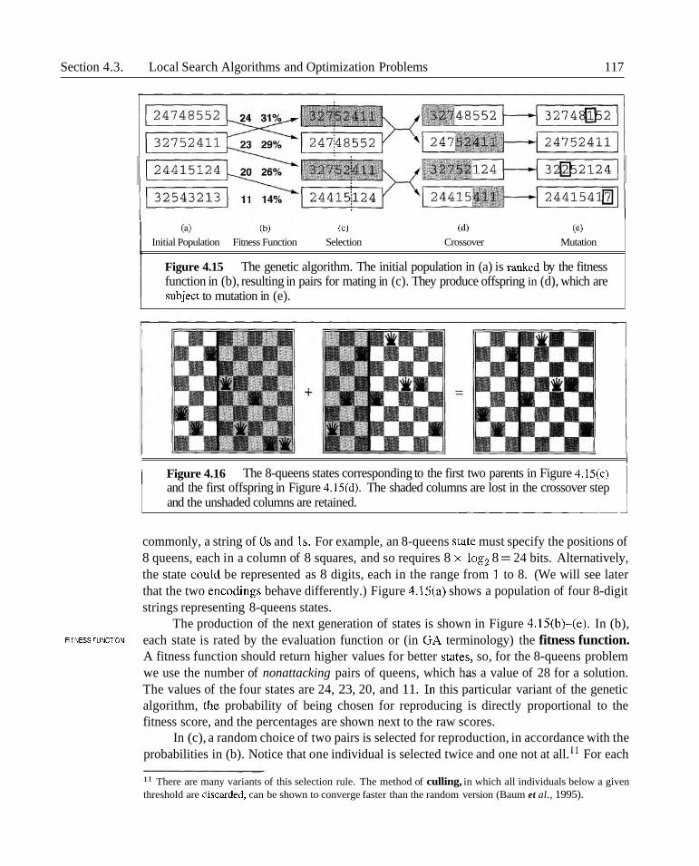
Figure 4.15 The genetic algorithm. The initial population in (a) is raiked by the fitness function in (b), resulting in pairs for mating in (c). They produce offspring in (d), which are subject to mutation in (e).

/ Figure 4.16 The 8-queens states corresponding to the first two parents in Figure 4.15(c) I and the first offspring in Figure 4.15(d). The shaded columns are lost in the crossover step and the unshaded columns are retained.

commonly, a string of 0s and 1s. For example, an 8-queens state must specify the positions of 8 queens, each in a column of 8 squares, and so requires 8 x logz 8 = 24 bits. Alternatively, the state clould be represented as 8 digits, each in the range from 1 to 8. (We will see later that the two encoding behave differently.) Figure 4.15(a) shows a population of four 8-digit strings representing 8-queens states.

The production of the next generation of states is shown in Figure 4.15(b)-(e). In (b), FITNESSFUNCTION each state is rated by the evaluation function or (in C;A terminology) the fitness function.

A fitness function should return higher values for better states, so, for the 8-queens problem we use the number of nonattacking pairs of queens, which has a value of 28 for a solution. The values of the four states are 24, 23, 20, and 11. Iin this particular variant of the genetic algorithm, ithe probability of being chosen for reproducing is directly proportional to the fitness score, and the percentages are shown next to the raw scores.

In (c), a random choice of two pairs is selected for reproduction, in accordance with the probabilities in (b). Notice that one individual is selected twice and one not at all. 'l For each

l1 There are many variants of this selection rule. The method of culling, in which all individuals below a given threshold are dliscarded, can be shown to converge faster than the random version (Baum et al., 1995).


CROSSOVER pair to be mated, a crossover point is randomly chosen from the positions in the string. In Figure 4.15 the crossover points are after the third digit in the first pair and after the fifth digit in the second pair. l2

In (d), the offspring themselves are created by crossing over the parent strings at the crossover point. For example, the first child of the first pair gets the first three digits from the first parent and the remaining digits from the second parent, whereas the second child gets the first three digits from the second parent and the rest from the first parent. The %queens states involved in this reproduction step are shown in Figure 4.16. The example illustrates the fact that, when two parent states are quite different, the crossover operation can produce a state that is a long way from either parent state. It is often the case that the population is quite diverse early on in the process, so crossover (like simulated annealing) frequently takes large steps in the state space early in the search process and smaller steps later on when most individuals are quite similar.

MUTATION Finally, in (e), each location is subject to random mutation with a small independent probability. One digit was mutated in the first, third, and fourth offspring. In the 8-queens problem, this corresponds to choosing a queen at random and moving it to a random square in its column. Figure 4.17 describes an algorithm that implements all these steps.

Like stochastic beam search, genetic algorithms combine an uphill tendency with random exploration and exchange of information among parallel search threads. The primary advantage, if any, of genetic algorithms comes from the crossover operation. Yet it can be shown mathematically that, if the positions of the genetic code is permuted initially in a random order, crossover conveys no advantage. Intuitively, the advantage comes from the ability of crossover to combine large blocks of letters that have evolved independently to perform useful functions, thus raising the level of granularity at which the search operates. For example, it could be that putting the first three queens in positions 2, 4, and 6 (where they do not attack each other) constitutes a useful block that can be combined with other blocks to construct a solution.

SCHEMA The theory of genetic algorithms explains how this works using the idea of a schema, which is a substring in which some of the positions can be left unspecified. For example, the schema 246""""" describes all 8-queens states in which the first three queens are in positions 2, 4, and 6 respectively. Strings that match the schema (such as 24613578) are called instances of the schema. It can be shown that, if the average fitness of the instances of a schema is above the mean, then the number of instances of the schema within the population will grow over time. Clearly, this effect is unlikely to be significant if adjacent bits are totally unrelated to each other, because then there will be few contiguous blocks that provide a consistent benefit. Genetic algorithms work best when schemas correspond to meaningful components of a solution. For example, if the string is a representation of an antenna, then the schemas may represent components of the antenna, such as reflectors and deflectors. A good component is likely to be good in a variety of different designs. This suggests that successful use of genetic algorithms requires careful engineering of the representation.

l2 It is here that the encoding matters. If a 24-bit encoding is used instead of 8 digits, then the crossover point has a 213 chance of being in the middle of a digit, which results in an essentially arbitrary mutation of that digit.

Section 4.4. Local Search in Continuous Spaces 119

function ~~ENETIC-ALGORITHM(~O~U~U~~O~, FITNESS-FN) returns an individual inputs: population, a set of individuals

FITNESS-FN, a function that measures the fitn'ess of an individual

repeat new-population t empty set loop for i from 1 to S~zE(popu~a t ion) do

x t R ~ ~ ~ o ~ - S ~ ~ ~ c ~ ~ o ~ ( p o p u l a t i o n , FITNESS-FN) y +- R A N D ~ M - ~ E L E C T I ~ N ( ~ ~ ~ U ~ ~ ~ ~ ~ ~ , FITNESS-FN) child +- REPRODUCE(X, y) if (small random probability) then child t M~rT~TE(chi1d) add child to new-population

population c new-popu2ation until some individual is fit enough, or enough time has elapsed return the best individual in population, according to FITNESS-FN

function REPRODUCE(X, y) returns an individual inputs: x , y, parent individuals

n t LENGTH($) c c random number from 1 to n return A P P E N D ( ~ U B S T R I N G ( X , 1 , c), SUBSTRING(^, c + 1, n ) )

Figure 4.17 A genetic algorithm. The algorithm is; the same as the one diagrammed in Figure 4.15, with one variation: in this more popular version, each mating of two parents produces only one offspring, not two.

In practice, genetic algorithms have had a widespread impact on optimization problems, such as circuit layout and job-shop scheduling. At present, it is not clear whether the appeal of genetic algorithms arises from their performance or from their aesthetically pleasing origins in the theory of evolution. Much work remains to be done to identify the conditions under which genetic algorithms perform well.

In Chapter 2, we explained the distinction between discrete and continuous environments, pointing out that most real-world environments are co~itinuous. Yet none of the algorithms we have described can handle continuous state spaces-the successor function would in most cases return infinitely many states! This section provides a very brief introduction to some local search techniques for finding optimal solutions in continuous spaces. The literature on this topic is vast; many of the basic techniques originated in the 17th century, after the development of calculus by Newton and ~e ibn iz . ' ~ We will find uses for these techniques at

l3 A basic knowledge of multivariate calculus and vector arithmetic is useful when one is reading this section.


EVOLUTION AND SEARCH

The theory of evolution was developed in Charles Darwin's On the Origin of Species by Means of Natural Selection (1859). The central idea is simple: variations (known as mutations) occur in reproduction and will be preserved in succes- sive generations approximately in proportion to their effect on reproductive fitness.

Darwin's theory was developed with no knowledge of how the traits of organisms can be inherited and modified. The probabilistic laws governing these pro- cesses were first identified by Gregor Mendel (1866), a monk who experimented with sweet peas using what he called artificial fertilization. Much later, Watson and Crick (1953) identified the structure of the DNA molecule and its alphabet, AGTC (adenine, guanine, thymine, cytosine). In the standard model, variation occurs both by point mutations in the letter sequence and by "crossover" (in which the DNA of an offspring is generated by combining long sections of DNA from each parent).

The analogy to local search algorithms has already been described; the princi- pal difference between stochastic beam search and evolution is the use of sexual reproduction, wherein successors are generated from multiple organisms rather than just one. The actual mechanisms of evolution are, however, far richer than most genetic algorithms allow. For example, mutations can involve reversals, duplica- tions, and movement of large chunks of DNA; some viruses borrow DNA from one organism and insert it in another; and there are transposable genes that do nothing but copy themselves many thousands of times within the genome. There are even genes that poison cells from potential mates that do not carry the gene, thereby increasing their chances of replication. Most important is the fact that the genes themselves encode the mechanisms whereby the genome is reproduced and trans- lated into an organism. In genetic algorithms, those mechanisms are a separate program that is not represented within the strings being manipulated.

Darwinian evolution might well seem to be an inefficient mechanism, having generated blindly some or so organisms without improving its search heuristics one iota. Fifty years before Darwin, however, the otherwise great French natu- ralist Jean Lamarck (1809) proposed a theory of evolution whereby traits acquired by adaptation during an organism's lifetime would be passed on to its offspring. Such a process would be effective, but does not seem to occur in nature. Much later, James Baldwin (1 896) proposed a superficially similar theory: that behavior learned during an organism's lifetime could accelerate the rate of evolution. Unlike Lamarck's, Baldwin's theory is entirely consistent with Darwinian evolution, because it relies on selection pressures operating on individuals that have found local optima among the set of possible behaviors allowed by their genetic makeup. Mod- ern computer simulations confirm that the "Baldwin effect" is real, provided that "ordinary" evolution can create organisms whose internal performance measure is somehow correlated with actual fitness.

Section 4.4. Local Search in Continuous Spaces 121

several places in the book, including the chapters on learning, vision, and robotics. In short, anything th~at deals with the real world.

Let us begin with an example. Suppose we want to place three new airports anywhere in Romania, such that the sum of squared distances from each city on the map (Figure 3.2) to its nearest airport is minimized. Then the state space i~s defined by the coordinates of the airports: (xl, yl), (x2, y2), and (x3, y3). This is a six-dimensional space; we also say that states ,we defined by six variables. (In general, states are defined by an n-dimensional vector of variables, x.) Moving around in this space corresponds to moving one or more of the airports on the map. The objective function f (xl , yl , x:~, yz, 2 3 , ys) is relatively easy to compute for any particular state once we compute the closest cities, but rather tricky to write down in general.

One way to avoid continuous problems is simply to discretize the neighborhood of each state. For example, we can move only one airport at a time in either the x or y direction by a fixed amount f 6. With 6 variables, this gives 12 possible successors for each state. We can then apply any of the local search algorithms described previously. One can also apply stochastic hill climbing and simulated annealing directly, without discretizing the space. These algorithms choose successors randomly, which can be done by generating random vec- tors of length 6.

GRADIENT There are many methods that attempt to use the gradient of the landscape to find a maximum. The gradient of the objective function is a vector V f that gives the magnitude and direction of the steepest slope. For our problem, we have

In some cases, we can find a maximum by solving the equation V f = 0. (This could be done, for example, if we were placing just one airport; the solution is the arithmetic mean of all the cities' coordinates.) In many cases, however, this equation cannot be solved in closed form. For example, with three airports, the expression for the gradient depends on what cities are closest to each airport in the current state. This means we can compute the gradient locally but not globally. Even so, we can still perform steepest-ascent hill climbing by updating the current state via the formula

where a is a small constant. In other cases, the obje'ctive function might not be available in a differentiable form at all-for example, the value of a particular set of airport locations may be determined by running some large-scale ecoinomic simulation package. In those

EMPIRICAL GRADIENT cases, a so-,called empirical gradient can be determined by evaluating the response to small

increments and decrements in each coordinate. Empirical gradient search is the same as steepest-ascent hill climbing in a discretized version of the state space.

Hidden beneath the phrase "a is a small consta.n.t9' lies a huge variety of methods for adjusting a . The basic problem is that, if a is too small, too many steps are needed; if a

LINE SEARCH is too large, the search could overshoot the maximum. The technique of line search tries to overcome this dilemma by extending the current gradient direction-usually by repeatedly doubling a-until f starts to decrease again. The point at which this occurs becomes the new


current state. There are several schools of thought about how the new direction should be chosen at this point.

NEWON-RAPHSON For many problems, the most effective algorithm is the venerable Newton-Raphson method (Newton, 1671; Raphson, 1690). This is a general technique for finding roots of functions-that is, solving equations of the form g(x) = 0. It works by computing a new estimate for the root x according to Newton's formula

To find a maximum or minimum of f, we need to find x such that the gradient is zero (i.e., Of(x) = 0). Thus g(x) in Newton's formula becomes V f (x), and the update equation can be written in matrix-vector form as

x +- x - H,'(x)v f (x) , HESSIAN where Hj(x) is the Hessian matrix of second derivatives, whose elements Hij are given

by a2 f /axiaxj. Since the Hessian has n2 entries, Newton-Raphson becomes expensive in high-dimensional spaces, and many approximations have been developed.

Local search methods suffer from local maxima, ridges, and plateaux in continuous state spaces just as much as in discrete spaces. Random restarts and simulated annealing can be used and are often helpful. High-dimensional continuous spaces are, however, big places in which it is easy to get lost.

CONSTRAINED OPTIMIZATION A final topic with which a passing acquaintance is useful is constrained optimization.

An optimization problem is constrained if solutions must satisfy some hard constraints on the values of each variable. For example, in our airport-siting problem, we might constrain sites to be inside Romania and on dry land (rather than in the middle of lakes). The difficulty of constrained optimization problems depends on the nature of the constraints and the objec-

LINEAR tive function. The best-known category is that of linear programming problems, in which constraints must be linear inequalities forming a convex region and the objective function is also linear. Linear programming problems can be solved in time polynomial in the number of variables. Problems with different types of constraints and objective functions have also been studied-quadratic programming, second-order conic programming, and so on.

4.5 ONLINE SEARCH AGENTS AND UNKNOWN ENVIRONMENTS

OFFLINESEARCH SO far we have concentrated on agents that use offline search algorithms. They compute a complete solution before setting foot in the real world (see Figure 3. I), and then execute the

ONLINE SEARCH solution without recourse to their percepts. In contrast, an online search14 agent operates by interleaving computation and action: first it takes an action, then it observes the environment and computes the next action. Online search is a good idea in dynamic or semidynamic domains-domains where there is a penalty for sitting around and computing too long. On- line search is an even better idea for stochastic domains. In general, an offline search would - -

l4 The term "online" is commonly used in computer science to refer to algorithms that must process input data as they are received, rather than waiting for the entire input data set to become available.

Section 4.5. Online Search Agents and Unknown Environments 123

have to come up with an exponentially large continger~cy plan that considers all possible hap- penings, while an online search need only consider what actually does happen. For example, a chess playing agent is well-advised to make its first move long before it has figured out the complete course of the game.

Online search is a necessary idea for an exploratiorn problem, where the states and actions are unknown to the agent. An agent in this state of Ignorance must use its actions as experiments to determine what to do next, and hence must interleave computation and action.

The canonical example of online search is a robot that is placed in a new building and must explore it to build a map that it can use for getting froin A to B. Methods for escaping from labyrinths-required knowledge for aspiring heroes of antiquity-are also examples of online search algorithms. Spatial exploration is not tlhe only form of exploration, however. Consider a newborn baby: it has many possible actions, but knows the outcomes of none of them, and it has experienced only a few of the possib~le states that it can reach. The baby's gradual discovery of how the world works is, in part, am online search process.

Online search problems

An online search problem can be solved only by an agent executing actions, rather than by a purely computational process. We will assume that the agent knows just the following:

ACTIONS(S), which returns a list of actions allowed in state s ; The step-cost function c(s , a , sl)-note that this cannot be used until the agent knows that sf is the outcome; and GOAL-TEST(S).

Note in particular that the agent cannot access the successors of a state except by actually trying all the actions in that state. For example, in the maze problem shown in Figure 4.18, the agent does not know that going Up from ( 1 , l ) leads to (1,2); nor, having done that, does it know that going Down will take it back to (1,l). This degree of ignorance can be reduced in some applications-for example, a robot explorer might know how its movement actions work and be ignorant only of the locations of obstacles.

We wrll assume that the agent can always recognize a state that it has visited before, and we will assume that the actions are deterministic. (These last two assumptions are relaxed in Chapter 17.) Finally, the agent might have access to an ,sdmissible heuristic function h(s) that estimates the distance from the current state to a goal state. For example, in Figure 4.18, the agent might know the location of the goal and be able to use the Manhattan distance heuristic.

Typically, the agent's objective is to reach a goal state while minimizing cost. (Another possible objective is simply to explore the entire environment.) The cost is the total path cost of the path that the agent actually travels. It is common to compare this cost with the path cost of the path the agent would follow if it knew the search space in advance-that is, the actual shortest path (or shortest complete exploration). In the language of online algorithms,

COMPETITIVE RATIO this is called the competitive ratio; we would like it to be as small as possible. Although this sounds like a reasonable request, it is easy to see that the best achievable

competitive ratio is infinite in some cases. For example,, if some actions are irreversible, the online search might accidentally reach a dead-end state from which no goal state is reachable.


1 2 3

Figure 4.18 A simpIe maze problem. The agent starts at S and must reach G, but knows nothing of the environment.

(a> (b)

Figure 4.19 (a) Two state spaces that might lead an online search agent into a dead end. Any given agent will fail in at least one of these spaces. (b) A two-dimensional environment that can cause an online search agent to follow an arbitrarily inefficient route to the goal. Whichever choice the agent makes, the adversary blocks that route with another long, thin wall, so that the path followed is much longer than the best possible path.

Perhaps you find the term "accidentally" unconvincing-after all, there might be an algorithm that happens not to take the dead-end path as it explores. Our claim, to be more precise, is that no algorithm can avoid dead ends in all state spaces. Consider the two dead-end state spaces in Figure 4.19(a). To an online search algorithm that has visited states S and A, the two state spaces look identical, so it must make the same decision in both. Therefore, it will fail in

ADVERSARY ARGUMENT one of them. This is an example of an adversary argument-we can imagine an adversary

that constructs the state space while the agent explores it and can put the goals and dead ends wherever it likes.


Dead ends are a real difficulty for robot exploration--staircases, ramps, cliffs, and all kinds of natural terrain present opportunities for irreversible actions. To make progress, we

SAFELY EXPLORABLE will simply assume that the state space is safely explorable-that is, some goal state is reachable from every reachable state. State spaces with reversible actions, such as mazes and 8-puzzles, can be viewed as undirected graphs and are clearly safely explorable.

Even in safely explorable environments, no bounded competitive ratio can be guaranteed if there are paths of unbounded cost. This is easy to show in environments with irreversible actions, but in fact it remains true for the reversible case as well, as Figure 4.19(b) shows. For this reason, it is common to describe the performance of online search algorithms in terms of the size of the entire state space rather than just the depth of the shallowest goal.

Online search agents

After each action, an online agent receives a percept telling it what state it has reached; from this information, it can augment its map of the environment. The current map is used to decide where to go next. This interleaving of planning and action means that online search algorithms are quite different from the offline search algorithms we have seen previously. For example, offline algorithms such as A* have the ability to expand a node in one part of the space and then immediately expand a node in ainother part of the space, because node expansion involves simulated rather than real actions. An online algorithm, on the other hand, can expand only a node that it physically occupies. To avoicl traveling all the way across the tree to expand the next node, it seems better to expand nodes in a local order. Depth-first search has exactly this property, because (except when backtracking) the next node expanded is a child of the previous node expanded.

An online depth-first search agent is shown in Figure 4.20. This agent stores its map in a table, result[a, s], that records the state resulting from executing action a in state s. Whenever an action from the current state has not been explored, the agent tries that action. The difficulty comes when the agent has tried all the actions in a state. In offline depth-first search, the state is simply dropped from the queue; in an online search, the agent has to backtrack physically. In depth-first search, this means going back to the state from which the agent entered the current state most recently. That is achieved by keeping a table that lists, for each state, the predecessor states to which the agent has riot yet backtracked. If the agent has run out of states to which it can backtrack, then its search is complete.

We recommend that the reader trace through the progress of ONLINE-DFS-AGENT

when applied to the maze given in Figure 4.18. It is fairly easy to see that the agent will, in the worst case, end up traversing every link in the state space exactly twice. For exploration, this is optimal; for finding a goal, on the other hand, the agent's competitive ratio could be arbitrarily bad if it goes off on a long excursion when there is a goal right next to the initial state. An online variant of iterative deepening solves this problem; for an environment that is a uniform tree, the competitive ratio of such an agent is a small constant.

Because of its method of backtracking, ONLINE-DFS-AGENT works only in state spaces where the actions are reversible. There are slightly more complex algorithms that work in general state spaces, but no such algorithm has a bounded competitive ratio.


function ONLINE-DFS-AGENT(S' ) returns an action inputs: s', a percept that identifies the current state static: result, a table, indexed by action and state, initially empty

unexplored, a table that lists, for each visited state, the actions not yet tried un.backtracked, a table that lists, for each visited state, the backtracks not yet tried s , a , the previous state and action, initially null

if GOAL-TEST(S') then return stop if s' is a new state then unexp1ored[s1] t ACTIONS(S ' ) if s is not null then do

result[a, s] +- s' add s to the front of unbacktracked[sl]

if unexplored[s

f

] is empty then if unbacktracked[s

f

] is empty then return stop else a +- an action b such that result[b, s

f

] = P~~(unbacktracked[s '] ) else a t Po~(unezplored[s']) s c s ' return a

Figure 4.20 An online search agent that uses depth-first exploration. The agent is applicable only in bidirected search spaces.

Online local search

Like depth-first search, hill-climbing search has the property of locality in its node expan- sions. In fact, because it keeps just one current state in memory, hill-climbing search is already an online search algorithm! Unfortunately, it is not very useful in its simplest form because it leaves the agent sitting at local maxima with nowhere to go. Moreover, random restarts cannot be used, because the agent cannot transport itself to a new state.

RANDOM WALK Instead of random restarts, one might consider using a random walk to explore the environment. A random walk simply selects at random one of the available actions from the current state; preference can be given to actions that have not yet been tried. It is easy to prove that a random walk will eventually find a goal or complete its exploration, provided that the space is finite.15 On the other hand, the process can be very slow. Figure 4.21 shows an environment in which a random walk will take exponentially many steps to find the goal, because, at each step, backward progress is twice as likely as forward progress. The example is contrived, of course, but there are many real-world state spaces whose topology causes these kinds of "traps" for random walks.

Augmenting hill climbing with memory rather than randomness turns out to be a more effective approach. The basic idea is to store a "current best estimate" H ( s ) of the cost to reach the goal from each state that has been visited. H ( s ) starts out being just the heuristic

l5 The infinite case is much more tricky. Random walks are complete on infinite one-dimensional and two dimensional grids, but not on three-dimensional grids! In the latter case, the probability that the walk ever returns to the starting point is only about 0.3405. (See Hughes, 1995, for a general introduction.)


S c G c v Figure 4.21 An environment in which a random walk will take exponentially many steps to find the goal.

estimate h ( s ) and is updated as the agent gains experience in the state space. Figure 4.22 shows a simple example in a one-dimensional state space. In (a), the agent seems to be stuck in a flat local minimum at the shaded state. Rather than staying where it is, the agent should follow what seems to be the best path to the goal based on the current cost estimates for its neighbors. The estimated cost to reach the goal through a neighbor s

f

is the cost to get to s

f

plus the estimated cost to get to a goal from there-that is, c(s , a, s

f

) + H ( s t ) . In the example, there are two actions with estimated costs 1 + 9 and 1 + 2, so it seems best to move right. Now, it is clear that the cost estimate of 2 for the shaded state was overly optimistic. Since the best move cost 1 and led to a state that is at least 2 steps from a goal, the shaded state must be at least 3 steps from a goal, so its H should be updated accordingly, as shown in Figure 4.22(b). Continuing this process, the agent will move back and forth twice more, updating H each time and "flattening out" the local minimum until it escapes to the right.

LRTA' An agent implementing this scheme, which is callled learning real-time A* (LRTA*), is shown in Figure 4.23. Like ONLINE-DFS-AGENT, it builds a map of the environment using the result table. It updates the cost estimate for the state it has just left and then chooses the "apparently best" move according to its current cost estimates. One important detail is that actions that have not yet been tried in a state s are always assumed to lead immediately to the

tirC:Ml$DER goal with the least possible cost, namely h ( s ) . This optimism under uncertainty encourages the agent to explore new, possibly promising paths.

An LRTA* agent is guaranteed to find a goal in any finite, safely explorable environment. Unlike A*, however, it is not complete for infinite state spaces--there are cases where it can be led infinitely astray. It can explore an environment of n states in O(n2) steps in the worst case, but often does much better. The LRTA* agent is just one of a large family of online agents that can be defined by specifying the action selection rule and the update rule in different ways. We will disc,uss this family, which was developed originally for stochastic environments, in Chapter 21.

Learning in online search

The initial ignorance of online search agents provides several opportunities for learning. First, the agents learn a "map" of the environment-more precisely, the outcome of each action in each state-simply by recording each of their experiences. (Notice that the assumption of deterministic environments means that one experience is enough for each action.) Second, the local search agents acquire more accurate estimates of the value of each state by using local updating mles, as in LRTA*. In Chapter 21 we will see that these updates eventually

128 Chapter 4. Informed Search and Exploration -- - -

Figure 4.22 Five iterations of LRTA* on a one-dimensional state space. Each state is labeled with H ( s ) , the current cost estimate to reach a goal, and each arc is labeled with its

1 step cost. The shaded state marks the location of the agent, and the updated values at each 1 iteration are circled.

function LRTA*-AGENT(S') returns an action inputs: st, a percept that identifies the current state static: result, a table, indexed by action and state, initially empty

H , a table of cost estimates indexed by state, initially empty s, a, the previous state and action, initially null

if GOAL-TEST(S') then return stop if s' is a new state (not in H ) then H[st] t h(st) unless s is null

result[a, s] +- st

H[s] t min LRTA*-COST(& b, result[b, s] , H ) b~ ACTIONS(S)

a t an action b in ACTIONS(S') that minimizes LRTA*-COST(S', b, result[b, s t] , H ) s t s t return a

function LRTA*-Cos~(s , a, s', H ) returns a cost estimate if st is undefined then return h ( s ) else return c(s, a, st) + H[st]

Figure 4.23 LRTA*-AGENT selects an action according to the values of neighboring states, which are updated as the agent moves about the state space.

Section 4.6. Summary 129

converge to exact values for every state, provided that the agent explores the state space in the right way. Once exact values are known, optimal decisi~ons can be taken simply by moving to the highest-valued successor-that is, pure hill climbing is then an optimal strategy.

If you followed our suggestion to trace the behavior of ONLINE-DFS- AGENT in the environment of Figure 4.18, you will have noticed that the agent is not very bright. For example, after it has seen that the Up action goes from (1,l) to (1,2), the agent still has no idea that the Down action goes back to (1,1), or that rthe Ujq action also goes from (2,l) to (2,2), from (2,2) to (2,3), and so on. In general, we would like the agent to learn that Up increases the y-coordinate unless there is a wall in the way, that Down reduces it, and so on. For this to happen, we need two things. First, we need a formal and explicitly manipulable representation for these kinds of general rules; so far, cve have hidden the information inside the black box called the successor function. Part I11 is devoted to this issue. Second, we need algorithms that can construct suitable general rules from the specific observations made by the agent. These are covered in Chapter 18.

This chapter has examined the application of heurist~ics to reduce search costs. We have looked at a number of algorithms that use heuristics and found that optimality comes at a stiff price in terns of search cost, even with good heuristics.

Best-first search is just GRAPH-SEARCH where the minimum-cost unexpanded nodes (according to some measure) are selected for expansion. Best-first algorithms typically use a heuristic function h(n) that estimates the cost of a solution from n.

0 Greedy best-first search expands nodes with minimal h(n). It is not optimal, but is often efficient.

A* search expands nodes with minimal f (n) = g(n) + h(n). A* is complete and optimal, provided that we guarantee that h(n) is admjssible (for TREE-SEARCH) or consistent (for GRAPH-SEARCH). The space complexity of A* is still prohibitive.

0 The performance of heuristic search algorithms dlepencls on the quality of the heuristic function. Good heuristics can sometimes be constructed by relaxing the problem definition, by precomputing solution costs for subproblems in a pattern database, or by learning from experience with the problem class.

RBFS and SMA* are robust, optimal search algorithms that use limited amounts of memory; given enough time, they can solve problems that A* cannot solve because it runs out of memory.

Local search methods such as hill climbing operate on complete-state formulations, keeping only a small number of nodes in memory. Several stochastic algorithms have been developed, including simulated annealing, which returns optimal solutions when given an appropriate cooling schedule. Many locall search methods can also be used to solve problems in continuous spaces.


A genetic algorithm is a stochastic hill-climbing search in which a large population of states is maintained. New states are generated by mutation and by crossover, which combines pairs of states from the population. Exploration problems arise when the agent has no idea about the states and actions of its environment. For safely explorable environments, online search agents can build a map and find a goal if one exists. Updating heuristic estimates from experience provides an effective method to escape from local minima.

BIBLIOGRAPHICAL AND HISTORICAL NOTES

The use of heuristic information in problem solving appears in an early paper by Simon and Newel1 (1958), but the phrase "heuristic search" and the use of heuristic functions that estimate the distance to the goal came somewhat later (Newell and Ernst, 1965; Lin, 1965). Doran and Michie (1966) conducted extensive experimental studies of heuristic search as applied to a number of problems, especially the 8-puzzle and the 15-puzzle. Although Doran and Michie carried out theoretical analyses of path length and "penetrance" (the ratio of path length to the total number of nodes examined so far) in heuristic search, they appear to have ignored the information provided by current path length. The A* algorithm, incorporating the current path length into heuristic search, was developed by Hart, Nilsson, and Raphael (1968), with some later corrections (Hart et al., 1972). Dechter and Pearl (1985) demonstrated the optimal efficiency of A*.

The original A* paper introduced the consistency condition on heuristic functions. The monotone condition was introduced by Pohl(1977) as a simpler replacement, but Pearl (1984) showed that the two were equivalent. A number of algorithms predating A* used the equivalent of open and closed lists; these include breadth-first, depth-first, and uniform-cost search (Bellman, 1957; Dijkstra, 1959). Bellman's work in particular showed the importance of additive path costs in simplifying optimization algorithms.

Pohl (1970, 1977) pioneered the study of the relationship between the error in heuristic functions and the time complexity of A*. The proof that A* runs in linear time if the error in the heuristic function is bounded by a constant can be found in Pohl (1977) and in Gaschnig (1979). Pearl (1984) strengthened this result to allow a logarithmic growth in the error. The "effective branching factor" measure of the efficiency of heuristic search was proposed by Nilsson (197 1).

There are many variations on the A* algorithm. Pohl(1973) proposed the use of dynamic weighting, which uses a weighted sum f,(n) = wgg(n) + whh(n) of the current path length and the heuristic function as an evaluation function, rather than the simple sum f (n) = g(n) + h(n ) used in A*. The weights wg and wh are adjusted dynamically as the search progresses. Pohl's algorithm can be shown to be E-admissible-that is, guaranteed to find solutions within a factor 1 + E of the optimal solution-where E is a parameter supplied to the algorithm. The same property is exhibited by the AT algorithm (Pearl, 1984), which can select any node from the fringe provided its f -cost is within a factor 1 + E of the lowest- f -cost fringe node. The selection can be done so as to minimize search cost.


A* arid other state-space search algorithms are closely related to the branch-and-bound techniques that are widely used in operations research (Lawler and Wood, 1966). The relationships between state-space search and branch-and-bound have been investigated in depth (Kumar and Kanal, 1983; Nau et al., 1984; Kuimar er al., 1988). Martelli and Monta- nari (1978) demonstrate a connection between dynamic programming (see Chapter 17) and certain types of state-space search. Kumar and Kanal (1988) attempt a "grand unification" of heuristic search, dynamic programming, and branch-and-bound techniques under the name of CDP-the "composite decision process."

Because computers in the late 1950s and early 1960s had at most a few thousand words of main memory, mernory-bounded heuristic search was an early research topic. The Graph Traverser (Doran and Michie, 1966), one of the earliest search programs, commits to an operator after searching best first up to the memory limit. IDA* (Korf, 1985a, 1985b) was the first widely used optimal, memory-bounded, heuristic search algorithm, and a large number of variants have been developed. An analysis of the efficiency of IDA* and of its difficulties with real-valued heuristics appears in Patrick et al. (1992).

RBFS (Korf, 1991, 1993) is actually somewhat more complicated than the algorithm shown in Figure 4.5, which is closer to an independently developed algorithm called iterative expansion, or IE (Russell, 1992). RBFS uses a lower bound as well as the upper bound; the two algoritl~ms behave identically with admissible heuristics, but RBFS expands nodes in best-first order even with an inadmissible heuristic. The idea of keeping track of the best alternative path appeared earlier in Bratko's (1986) elegant Yrolog implementation of and in the DTA* algorithm (Russell and Wefald, 1991). The latter work also discusses metalevel state spaces and metalevel learning.

The MA* algorithm appeared in Chakrabarti et 01. (1989). SMA*, or Simplified Mx, emerged from an attempt: to implement MA* as a comparison algorithm for IE (Russell, 1992). Kaindl and Khorsand (1994) have applied SMA* to produce a bidirectional search algorithm that is substantially faster than previous algorithms. Ko~f and Zhang (2000) describe a divide- and-conqueiW approach, and Zhou and Hansen (2002) i~ntroduce memory-bounded A* graph search. Korf (1995) surveys memory-bounded search techniques.

The idea that admissible heuristics can be derived by problem relaxation appears in the seminal paper by Held and Karp (1970), who used the the minimum-spanning-tree heuristic to solve the TSP. (See Exercise 4.8.)

The automation of the relaxation process was implemented successfully by Priedi- tis (1993), building on earlier work with Mostow (Mostow and Prieditis, 1989). The use of pattern databases to derive admissible heuristics is due to Gasser (1995) and Culberson and Schaeffer (1998); disjoint pattern datlabases are described by Korf and Felner (2002). The probabilistic interpretation of heuristics was investigated in depth by Pearl (1984) and Hansson and Mayer (1989).

By far the most comprehensive source on heuristics and heuristic search algorithms is Pearl's (1984) Heuristics text. This book provides especially good coverage of the wide variety of offshoots and variations of A*, including rigorous proofs of their formal properties. Kana1 and Kumar (1988) present an anthology of important articles on heuristic search. New results on search algorithms appear regularly in the journal Art$cial Intelligence.


Local-search techniques have a long history in mathematics and computer science. In- deed, the Newton-Raphson method (Newton, 1671; Raphson, 1690) can be seen as a very efficient local-search method for continuous spaces in which gradient information is available. Brent (1973) is a classic reference for optimization algorithms that do not require such information. Beam search, which we have presented as a local-search algorithm, originated as a bounded-width variant of dynamic programming for speech recognition in the HARPY

system (Lowerre, 1976). A related algorithm is analyzed in depth by Pearl (1984, Ch. 5). The topic of local search has been reinvigorated in recent years by surprisingly good

results for large constraint satisfaction problems such as n-queens (Minton et al., 1992) and logical reasoning (Selman et al., 1992) and by the incorporation of randomness, multiple simultaneous searches, and other improvements. This renaissance of what Christos Papadi- mitriou has called "New Age" algorithms has also sparked increased interest among theoretical computer scientists (Koutsoupias and Papadimitriou, 1992; Aldous and Vazirani, 1994).

TABU SEARCH In the field of operations research, a variant of hill climbing called tabu search has gained popularity (Glover, 1989; Glover and Laguna, 1997). Drawing on models of limited short- term memory in humans, this algorithm maintains a tabu list of k previously visited states that cannot be revisited; as well as improving efficiency when searching graphs, this can allow the algorithm to escape from some local minima. Another useful improvement on hill climbing is the STAGE algorithm (Boyan and Moore, 1998). The idea is to use the local maxima found by random-restart hill climbing to get an idea of the overall shape of the landscape. The algorithm fits a smooth surface to the set of local maxima and then calculates the global maximum of that surface analytically. This becomes the new restart point. The algorithm has been shown to work in practice on hard problems. (Gomes et al., 1998) showed that the run time distributions of systematic backtracking algorithms often have a heavy-tailed

HEAVY-TAILED olsTRleUrloN distribution, which means that the probability of a very long run time is more than would be predicted if the run times were normally distributed. This provides a theoretical justification for random restarts.

Simulated annealing was first described by arkpatrick et al. (1983), who borrowed directly from the Metropolis algorithm (which is used to simulate complex systems in physics (Metropolis et al., 1953) and was supposedly invented at a Los Alamos dinner party). Simulated annealing is now a field in itself, with hundreds of papers published every year.

Finding optimal solutions in continuous spaces is the subject matter of several fields, including optimization theory, optimal control theory, and the calculus of variations. Suitable (and practical) entry points are provided by Press et al. (2002) and Bishop (1995). Linear programming (LP) was one of the first applications of computers; the simplex algorithm (Wood and Dantzig, 1949; Dantzig, 1949) is still used despite worst-case exponential complexity. Karmarkar (1984) developed a practical polynomial-time algorithm for LP.

Work by Sewall Wright (1931) on the concept of a fitness landscape was an important precursor to the development of genetic algorithms. In the 1950s, several statisticians, including Box (1957) and Friedman (1959), used evolutionary techniques for optimization

EVOLUTION STRATEGIES

problems, but it wasn't until Rechenberg (1965, 1973) introduced evolution strategies to solve optimization problems for airfoils that the approach gained popularity. In the 1960s and 1970s, John Holland (1975) championed genetic algorithms, both as a useful tool and


as a method to expand our understanding of adaptation, biological or otherwise (Holland, ARTIFICIALLIFE 1995). The artificial life movement (Langton, 1995) takes this idea one step further, view-

ing the products of genetic algorithms as organisms rather than solutions to problems. Work in this field by Hinton and Nowlan (1987) and Ackley and Littman (1991) has done much to clarify the implications of the Baldwin effect. For general background on evolution, we strongly recommend Smith and Szathmhry (1999).

Most comparisons of genetic algorithms to other approaches (especially stochastic hill- climbing) have found that the genetic algorithms are slower to converge (O'Reilly and Op- pacher, 1994; Mitchell et al., 1996; Juels and Wattenberg, 1996; Baluja, 1997). Such findings are not universally popular within the GA communit:y, but recent attempts within that com- munity to understand population-based search as an approximate form of Bayesian learning (see Chapter 20) might help to close the gap between Ithe field and its critics (Pelikan et al., 1999). The theory of quadratic dynamical systems may also explain the performance of GAS (Rabani et aZ., 1998). See Lohn et al. (2001) for an example of GAS applied to antenna design, and Larrafiaga et al. (1999) for an application to the traveling salesperson problem.

GENETIC PROGRAMMING The field of genetic programming is closely related to genetic algorithms. The princi-

pal difference is that the representations that are mutated and combined are programs rather than bit strings. The programs are represented in the form of expression trees; the expressions can be in a standard language such as Lisp or can be specialty designed to represent circuits, robot controllers, and so on. Crossover involves splicing together subtrees rather than sub- strings. This form of mutation guarantees that the offspring are well-formed expressions, which would not be the case if programs were manipulated as strings.

Recent interest in genetic programming was spurred by John Koza's work (Koza, 1992, 1994), but it goes back at least to early experiments with machine code by Friedberg (1958) and with finite-state automata by Fogel et al. (1966). As with genetic algorithms, there is debate about the effectiveness of the technique. Koza et al. (1999) describe a variety of experiments on the automated design of circuit devices using genetic programming.

The journals Evolutionary Conzputation and IEEE Tran,sactions on Evolutionary Com- putation cover genetic algorithms and genetic progranlmning; articles are also found in Com- plex Systems, Adaptive Behavior, and Art$cial L$e. 'The main conferences are the Inter- national Conference on Genetic Algorithms and the Conference on Genetic Programming, recently merged to form the Genetic and Evolutionary Computation Conference. The texts by Melanie Mitchell (1996) and David Fogel (2000) give good overviews of the field.

Algorithms for exploring unknown state spaces have been of interest for many centuries. Depth-first search in a maze can be implemented by keeping one's left hand on the wall; loops can be avoided by marlung each junction. Depth-first search fails with irreversible actions; the

EULERIANGRAPHS more general problem of exploring of Eulerian graphs (i.e., graphs in which each node has equal numbers of incoming and outgoing edges) was solved by an algorithm due to Hierholzer (1873). The first thorough algorithmic study of the exploration problem for arbitrary graphs was carried out by Deng and Papadimitriou (1990), who developed a completely general algorithm, but showed that no bounded competitive ratilo is possible for exploring a general graph. Papadimitriou and Yannakalus (1991) examined the question of finding paths to a goal in geometric path-planning environments (where all actions are reversible). They showed that


a small competitive ratio is achievable with square obstacles, but with general rectangular obstacles no bounded ratio can be achieved. (See Figure 4.19.)

The LRTA* algorithm was developed by Korf (1990) as part of an investigation into REAL-TIMESEARCH real-time search for environments in which the agent must act after searching for only a

fixed amount of time (a much more common situation in two-player games). LRTA* is in fact a special case of reinforcement learning algorithms for stochastic environments (Barto et al., 1995). Its policy of optimism under uncertainty-always head for the closest unvisited state--can result in an exploration pattern that is less efficient in the uninformed case than simple depth-first search (Koenig, 2000). Dasgupta et al. (1994) show that online iterative deepening search is optimally efficient for finding a goal in a uniform tree with no heuristic information. Several informed variants on the LRTA* theme have been developed with different methods for searching and updating within the known portion of the graph (Pemberton and Korf, 1992). As yet, there is no good understanding of how to find goals with optimal efficiency when using heuristic information.

PARALLEL SEARCH The topic of parallel search algorithms was not covered in the chapter, partly because it requires a lengthy discussion of parallel computer architectures. Parallel search is becoming an important topic in both A1 and theoretical computer science. A brief introduction to the A1 literature can be found in Mahanti and Daniels (1993).

4.1 Trace the operation of A* search applied to the problem of getting to Bucharest from Lugoj using the straight-line distance heuristic. That is, show the sequence of nodes that the algorithm will consider and the f , g, and h score for each node.

4.2 The heuristic path algorithm is a best-first search in which the objective function is f ( n ) = (2 - w)g(n) + wh(n). For what values of w is this algorithm guaranteed to be optimal? (You may assume that h is admissible.) What kind of search does this perform when w = O? When w = l? When w = 2?

4.3 Prove each of the following statements:

a. Breadth-first search is a special case of uniform-cost search.

b. Breadth-first search, depth-first search, and uniform-cost search are special cases of best-first search.

c. Uniform-cost search is a special case of A* search.

1-p 4.4 Devise a state space in which A* using GRAPH-SEARCH returns a suboptimal solution with an h(n) function that is admissible but inconsistent.

4.5 We saw on page 96 that the straight-line distance heuristic leads greedy best-first search astray on the problem of going from Iasi to Fagaras. However, the heuristic is perfect on the opposite problem: going from Fagaras to Iasi. Are there problems for which the heuristic is misleading in both directions?


4.6 Invent a heuristic function for the 8-puzzle that sometirnes overestimates, and show how it can lead to a suboptimal solution on a particular problem. (You can use a computer to help if you want.) Prove that, if h never overestimates by more than c, A* using h returns a solution whose cost exceeds that of the optimal solution by no more than c.

4.7 Prove that if a heuristic is consistent, it must be admissible. Construct an admissible heuristic that is not consistent.

4.8 The traveling salesperson problem (TSP) can be solved via the minimum spanning tree (MST) heuristic, which is used to estimate the cost of completing a tour, given that a partial tour has already been constructed. The MST cost of a set of cities is the smallest sum of the link costs of any tree that connects all the cities.

a. Show how this heuristic can be derived from a relaxed version of the TSP.

b. Show that the MST heuristic dominates straight-:line distance.

c. Write a problem generator for instances of the TSP where cities are represented by random points in the unit square.

d. Find an efficient algorithm in the literature for constructing the MST, and use it with an admissible search algorithm to solve instances of the TSP.

4.9 On page 108, we defined the relaxation of the &-puzzle in which a tile can move from square A to square B if B is blank. The exact solution of this problem defines Gaschnig's heuristic (Gaschnig, 1979). Explain why Gaschnig's heuristic is at least as accurate as hl (misplaced tiles), and show cases where it is more accurate than both hl and h2 (Manhattan distance). Can you suggest a way to calculate Gaschnig's heuristic efficiently?

1-ia 4.10 We gave two simple heuristics for the 8-puzzle:: Manhattan distance and misplaced tiles. Several heuristics in the literature purport to improve on this-see, for example, Nils- son (1971), Mostow and Prieditis (1989), and Hansson et al. (1992). Test these claims by implementing the heuristics and comparing the perform;znce of the resulting algorithms.

4.11 Give the name of the algorithm that results from each of the following special cases:

a. Local beam search with k = 1.

b. Local beam search with one initial state and no limit on the number of states retained.

c. Simulated annealing with T = 0 at all times (and omitting the termination test).

d. Genetic algorithm with population size N = 1.

4.12 Sometimes there is no good evaluation function for a problem, but there is a good comparison method: a way to tell whether one node is better than another, without assigning numerical values to either. Show that this is enough to do a best-first search. Is there an analog of A*?

4.13 Relate the time complexity of LRTA* to its space complexity.

4.14 Suppose that an agent is in a 3 x 3 maze environment like the one shown in Fig- ure 4.18. The agent knows that its initial location is (1,1)1, that the goal is at (3 ,3) , and that the


four actions Up, Down, Left, Right have their usual effects unless blocked by a wall. The agent does not know where the internal walls are. In any given state, the agent perceives the set of legal actions; it can also tell whether the state is one it has visited before or a new state.

a. Explain how this online search problem can be viewed as an offline search in belief state space, where the initial belief state includes all possible environment configurations. How large is the initial belief state? How large is the space of belief states?

b. How many distinct percepts are possible in the initial state?

c. Describe the first few branches of a contingency plan for this problem. How large (roughly) is the complete plan?

Notice that this contingency plan is a solution for every possible environment fitting the given description. Therefore, interleaving of search and execution is not strictly necessary even in unknown environments.

\@i@Ep 4.15 In this exercise, we will explore the use of local search methods to solve TSPs of the type defined in Exercise 4.8.

a. Devise a hill-climbing approach to solve TSPs. Compare the results with optimal solutions obtained via the A* algorithm with the MST heuristic (Exercise 4.8).

b. Devise a genetic algorithm approach to the traveling salesperson problem. Compare results to the other approaches. You may want to consult Larraiiaga et al. (1999) for some suggestions for representations.

1giSjqF 4.16 Generate a large number of 8-puzzle and 8-queens instances and solve them (where possible) by hill climbing (steepest-ascent and first-choice variants), hill climbing with random restart, and simulated annealing. Measure the search cost and percentage of solved problems and graph these against the optimal solution cost. Comment on your results.

\ m p 4.17 In this exercise, we will examine hill climbing in the context of robot navigation, using the environment in Figure 3.22 as an example.

a. Repeat Exercise 3.16 using hill climbing. Does your agent ever get stuck in a local minimum? Is it possible for it to get stuck with convex obstacles?

b. Construct a nonconvex polygonal environment in which the agent gets stuck.

c. Modify the hill-climbing algorithm so that, instead of doing a depth-1 search to decide where to go next, it does a depth-k search. It should find the best k-step path and do one step along it, and then repeat the process.

d. Is there some k for which the new algorithm is guaranteed to escape from local minima?

e. Explain how LRTA* enables the agent to escape from local minima in this case.

I(gggiEp 4.18 Compare the performance of A* and RBFS on a set of randomly generated problems in the 8-puzzle (with Manhattan distance) and TSP (with MST-see Exercise 4.8) domains. Discuss your results. What happens to the performance of RBFS when a small random number is added to the heuristic values in the 8-puzzle domain?

4 exploration informed search and - uni...

Documents