4 grid generation - missouri s&tweb.mst.edu/~norbert/ge5471/assignments/assign 1 - flac...

GRID GENERATION 4 - 1

4 GRID GENERATION

4.1 General Comments

Unlike many modeling programs based on the finite element method, FLAC organizes its zones (or“elements”) in a row-and-column fashion, like a crossword puzzle. We refer to a particular zoneby a pair of numbers (its row and column numbers) rather than by an arbitrary ID number, as infinite element programs. Although the numbering scheme resembles that of a crossword puzzle,the physical shape of a FLAC grid need not be rectangular: the rows and columns can be distortedso that the boundary fits some given shape; holes can be made in the grid; and separate grids can bestuck together to create more complicated bodies. Furthermore, the zones can vary in size across agrid. This section describes the various ways in which FLAC grids can be made to fit the physicalshapes that are to be modeled.

When fairly simple shapes are to be modeled, FLAC ’s grid scheme is very easy to use and interpret.For one thing, printed output (such as a list of zone stresses) is arranged on the page in a way thatcorresponds closely with positions in physical space. In contrast, finite element output is arrangedarbitrarily. The advantages tend to vanish, however, as the objects to be modeled become morecomplicated. Some degree of skill is needed to set up complex grids.

With any numerical method, the accuracy of the results depends on the grid used to represent thephysical system. In general, finer meshes (more zones per unit length) lead to more accurate results.Furthermore, the aspect ratio (ratio of height to width of a zone) also affects accuracy. When creatinggrids with FLAC, it should be kept in mind that the greatest accuracy is obtained for a model withequal, square zones. If the model must contain different zone sizes, then a gradual variation insize should be used for maximum accuracy; this factor is important enough that a special option isprovided in the GENERATE command whereby zone sizes can be arranged to increase or decreaseby a constant ratio along any grid line. As a general rule, the aspect ratio of a zone should be keptas close to unity as possible: anything above 5:1 is potentially inaccurate. Section 3.2 in the User’sGuide provides some guidelines for choosing zone sizes and shapes, and some justification for therules just given. The purpose of this section is to show the reader what tools are available for gridgeneration, and how to use them effectively.

The discussion and examples provided in this section use the command-line approach to data inputto FLAC. You are encouraged to work through the examples in this section to become familiar withthe principles used for grid generation in FLAC.*

* The data files in this chapter are all created in a text editor. The files are stored in the directory“ITASCA\FLAC600\Theory\4-Grid” with the extension “.DAT.” A project file is also providedfor each example. In order to run an example and compare the results to plots in this chapter, open aproject file in the GIIC by clicking on the File / Open Project menu item and selecting the projectfile name (with extension “.PRJ”). Click on the Project Options icon at the top of the Project TreeRecord, select Rebuild unsaved states, and the example data file will be run and plots created.

FLAC Version 6.0

4 - 2 Theory and Background

Creation of grids, especially for complex model shapes, is greatly assisted by the graphical interface(the GIIC – see Section 2.2.1 in the User’s Guide and the FLAC-GIIC Reference volume). Allthe operations described in this section can be achieved via the GIIC. In addition, a grid libraryis provided; it contains grid objects commonly used in geomechanics: dam, retaining wall, tunnel,etc. The library objects are a useful starting point to construct a model.

A “virtual-grid” generation mode is also provided in the GIIC to facilitate grid creation. SeeSection 1.2.1 in the FLAC-GIIC Reference for a description of the virtual-grid mode of gridgeneration.

FLAC Version 6.0


4.2 Generation of Simple Shapes

The GRID command is of the form

grid p,q

It produces a grid of square zones, with p-zones in the x-direction and q-zones in the y-direction.The intersections of mesh lines are called gridpoints. By default, the x-coordinates of the gridpointsare 0, 1, . . . , p, and the y-coordinates are 0, 1, . . . , q. Note that there are (p + 1) vertical mesh linesand (q + 1) horizontal mesh lines.

In order to stretch, shrink or shift the grid in the x- or y-directions, the initialization command,INITIAL, can be used to modify the coordinates, using the parameters mul or add. The input line

ini x mul 2

multiplies all x-coordinates by a factor of two. The input line

ini x add 10

shifts the whole grid by 10 units in the x-direction. Combinations of these operations can be enteredon a single line. For example, the input line

ini x mul 2, y mul 2, x add 10

will enlarge the existing grid by a factor of two, and then shift it ten units in the x-direction. Notethat negative multiplication factors should not be used on coordinates because the “sense” of thegrid will be reversed, causing negative zone areas. This will trigger an error message later on, whena STEP command is given.

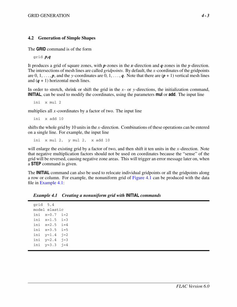
The INITIAL command can also be used to relocate individual gridpoints or all the gridpoints alonga row or column. For example, the nonuniform grid of Figure 4.1 can be produced with the datafile in Example 4.1:

Example 4.1 Creating a nonuniform grid with INITIAL commands

grid 5,4model elasticini x=0.7 i=2ini x=1.5 i=3ini x=2.5 i=4ini x=3.5 i=5ini y=1.4 j=2ini y=2.4 j=3ini y=3.3 j=4

FLAC Version 6.0


Figure 4.1 Nonuniform grid, using INITIAL commands

The command

initial x=0.7 i=2

sets all x-coordinates on the vertical grid line i=2 equal to 0.7 units. Similarly, the command

initial y=2.4 j=3

sets all y-coordinates on the horizontal grid line j = 3 equal to 2.4 units. Note that the commandMODEL elastic is not necessary for the process of changing coordinates, but it is given in order torender the grid visible when it is plotted via a PLOT grid command. If no model is specified, a“null” model, which plots as an empty space, is assumed.

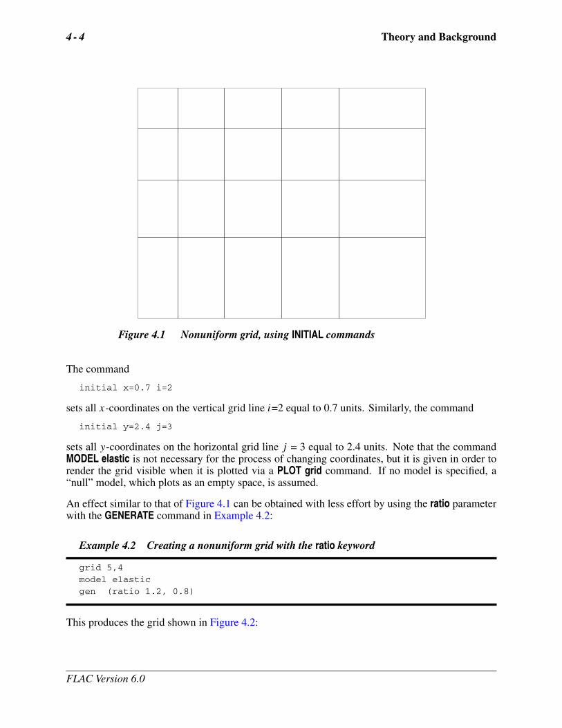
An effect similar to that of Figure 4.1 can be obtained with less effort by using the ratio parameterwith the GENERATE command in Example 4.2:

Example 4.2 Creating a nonuniform grid with the ratio keyword

grid 5,4model elasticgen (ratio 1.2, 0.8)

This produces the grid shown in Figure 4.2:

FLAC Version 6.0


Figure 4.2 Nonuniform grid, using the ratio keyword with the GENERATEcommand

In this grid, the widths of successive zones in the x-direction are increased by a factor of 1.2, andthe heights of successive zones in the y-direction are increased by a factor of 0.8 (i.e., decreased).On the matter of syntax, the brackets enclosing the ratio keyword and its parameters are optional:they are simply included for cosmetic reasons (see Section 1.1.1 in the Command Reference).

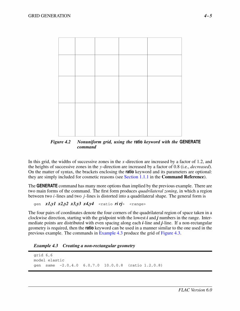
The GENERATE command has many more options than implied by the previous example. There aretwo main forms of the command. The first form produces quadrilateral zoning, in which a regionbetween two i-lines and two j -lines is distorted into a quadrilateral shape. The general form is

gen x1,y1 x2,y2 x3,y3 x4,y4 <ratio ri rj> <range>

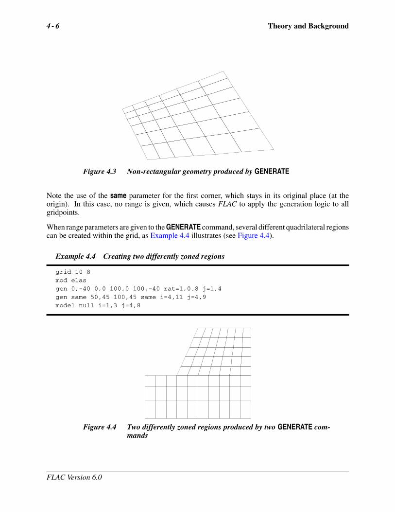
The four pairs of coordinates denote the four corners of the quadrilateral region of space taken in aclockwise direction, starting with the gridpoint with the lowest i and j numbers in the range. Inter-mediate points are distributed with even spacing along each i-line and j-line. If a non-rectangulargeometry is required, then the ratio keyword can be used in a manner similar to the one used in theprevious example. The commands in Example 4.3 produce the grid of Figure 4.3.

Example 4.3 Creating a non-rectangular geometry

grid 6,6model elasticgen same -2.0,4.0 6.0,7.0 10.0,0.8 (ratio 1.2,0.8)

FLAC Version 6.0


Figure 4.3 Non-rectangular geometry produced by GENERATE

Note the use of the same parameter for the first corner, which stays in its original place (at theorigin). In this case, no range is given, which causes FLAC to apply the generation logic to allgridpoints.

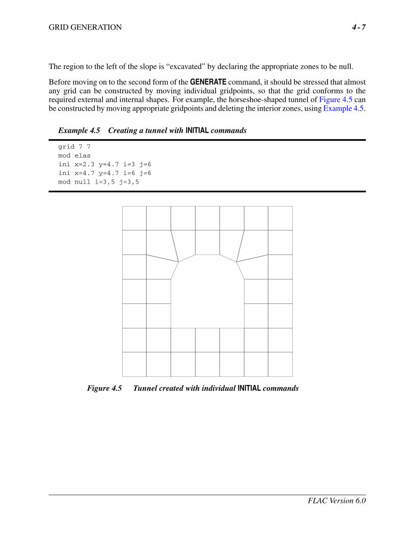
When range parameters are given to the GENERATE command, several different quadrilateral regionscan be created within the grid, as Example 4.4 illustrates (see Figure 4.4).

Example 4.4 Creating two differently zoned regions

grid 10 8mod elasgen 0,-40 0,0 100,0 100,-40 rat=1,0.8 j=1,4gen same 50,45 100,45 same i=4,11 j=4,9model null i=1,3 j=4,8

Figure 4.4 Two differently zoned regions produced by two GENERATE com-mands

FLAC Version 6.0


The region to the left of the slope is “excavated” by declaring the appropriate zones to be null.

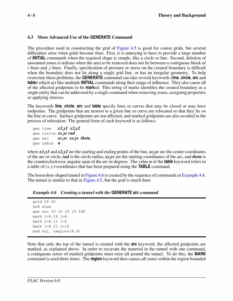
Before moving on to the second form of the GENERATE command, it should be stressed that almostany grid can be constructed by moving individual gridpoints, so that the grid conforms to therequired external and internal shapes. For example, the horseshoe-shaped tunnel of Figure 4.5 canbe constructed by moving appropriate gridpoints and deleting the interior zones, using Example 4.5.

Example 4.5 Creating a tunnel with INITIAL commands

grid 7 7mod elasini x=2.3 y=4.7 i=3 j=6ini x=4.7 y=4.7 i=6 j=6mod null i=3,5 j=3,5

Figure 4.5 Tunnel created with individual INITIAL commands

FLAC Version 6.0


4.3 More Advanced Use of the GENERATE Command

The procedure used in constructing the grid of Figure 4.5 is good for coarse grids, but severaldifficulties arise when grids become finer. First, it is annoying to have to provide a large numberof INITIAL commands when the required shape is simple, like a circle or line. Second, deletion ofunwanted zones is tedious when the area to be removed does not lie between a contiguous block ofi-lines and j -lines. Finally, specification of pressure or stress on the created boundary is difficultwhen the boundary does not lie along a single grid line, or has an irregular geometry. To helpovercome these problems, the GENERATE command can take several keywords (line, circle, arc andtable) which act like multiple INITIAL commands along their range of influence. They also cause allof the affected gridpoints to be marked. This string of marks identifies the created boundary as asingle entity that can be addressed by a single command when removing zones, assigning propertiesor applying stresses.

The keywords line, circle, arc and table specify lines or curves that may be closed or may haveendpoints. The gridpoints that are nearest to a given line or curve are relocated so that they lie onthe line or curve. Surface gridpoints are not affected, and marked gridpoints are also avoided in theprocess of relocation. The general form of each keyword is as follows:

gen line x1,y1 x2,y2gen circle xc,yc radgen arc xc,yc xs,ys thetagen table n

where x1,y1 and x2,y2 are the starting and ending points of the line, xc,yc are the center coordinatesof the arc or circle, rad is the circle radius, xs,ys are the starting coordinates of the arc, and theta isthe counterclockwise angular span of the arc in degrees. The value n of the table keyword refers toa table of (x,y)-coordinates that has been prepared using the TABLE command.

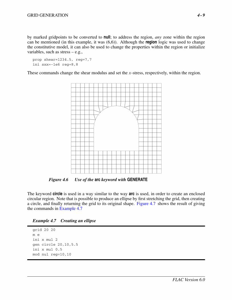
The horseshoe-shaped tunnel in Figure 4.6 is created by the sequence of commands in Example 4.6.The tunnel is similar to that in Figure 4.5, but the grid is much finer.

Example 4.6 Creating a tunnel with the GENERATE arc command

grid 20 20mod elasgen arc 10 10 15 10 180mark i=6,16 j=6mark j=6,11 i=6mark j=6,11 i=16mod nul, region=(6,6)

Note that only the top of the tunnel is created with the arc keyword; the affected gridpoints aremarked, as explained above. In order to excavate the material in the tunnel with one command,a contiguous series of marked gridpoints must exist all around the tunnel. To do this, the MARKcommand is used three times. The region keyword then causes all zones within the region bounded

FLAC Version 6.0


by marked gridpoints to be converted to null; to address the region, any zone within the regioncan be mentioned (in this example, it was (6,6)). Although the region logic was used to changethe constitutive model, it can also be used to change the properties within the region or initializevariables, such as stress – e.g.,

prop shear=1234.5, reg=7,7ini sxx=-1e6 reg=8,8

These commands change the shear modulus and set the x-stress, respectively, within the region.

Figure 4.6 Use of the arc keyword with GENERATE

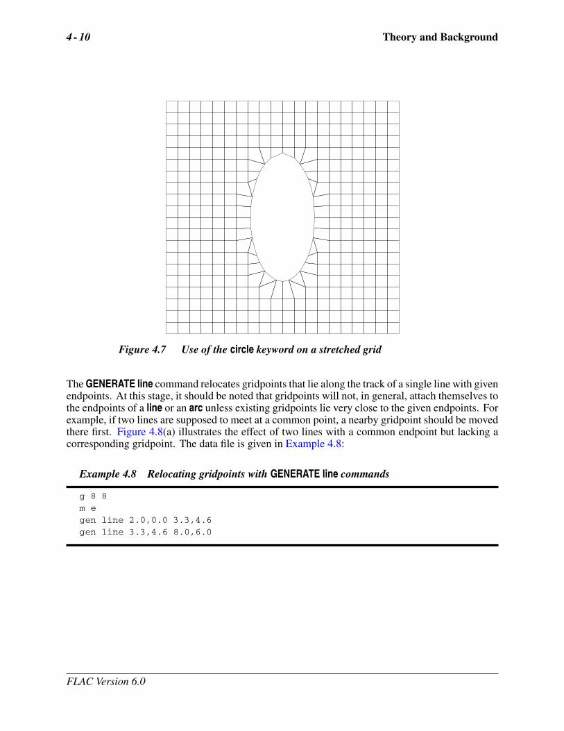
The keyword circle is used in a way similar to the way arc is used, in order to create an enclosedcircular region. Note that is possible to produce an ellipse by first stretching the grid, then creatinga circle, and finally returning the grid to its original shape. Figure 4.7 shows the result of givingthe commands in Example 4.7

Example 4.7 Creating an ellipse

grid 20 20m eini x mul 2gen circle 20,10,5.5ini x mul 0.5mod nul reg=10,10

FLAC Version 6.0


Figure 4.7 Use of the circle keyword on a stretched grid

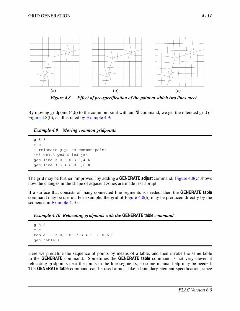
The GENERATE line command relocates gridpoints that lie along the track of a single line with givenendpoints. At this stage, it should be noted that gridpoints will not, in general, attach themselves tothe endpoints of a line or an arc unless existing gridpoints lie very close to the given endpoints. Forexample, if two lines are supposed to meet at a common point, a nearby gridpoint should be movedthere first. Figure 4.8(a) illustrates the effect of two lines with a common endpoint but lacking acorresponding gridpoint. The data file is given in Example 4.8:

Example 4.8 Relocating gridpoints with GENERATE line commands

g 8 8m egen line 2.0,0.0 3.3,4.6gen line 3.3,4.6 8.0,6.0

FLAC Version 6.0


(a) (b) (c)

Figure 4.8 Effect of pre-specification of the point at which two lines meet

By moving gridpoint (4,6) to the common point with an INI command, we get the intended grid ofFigure 4.8(b), as illustrated by Example 4.9:

Example 4.9 Moving common gridpoints

g 8 8m e; relocate g.p. to common pointini x=3.3 y=4.6 i=4 j=6gen line 2.0,0.0 3.3,4.6gen line 3.3,4.6 8.0,6.0

The grid may be further “improved” by adding a GENERATE adjust command. Figure 4.8(c) showshow the changes in the shape of adjacent zones are made less abrupt.

If a surface that consists of many connected line segments is needed, then the GENERATE tablecommand may be useful. For example, the grid of Figure 4.8(b) may be produced directly by thesequence in Example 4.10:

Example 4.10 Relocating gridpoints with the GENERATE table command

g 8 8m etable 1 2.0,0.0 3.3,4.6 8.0,6.0gen table 1

Here we predefine the sequence of points by means of a table, and then invoke the same tablein the GENERATE command. Sometimes the GENERATE table command is not very clever atrelocating gridpoints near the joints in the line segments, so some manual help may be needed.The GENERATE table command can be used almost like a boundary element specification, since

FLAC Version 6.0


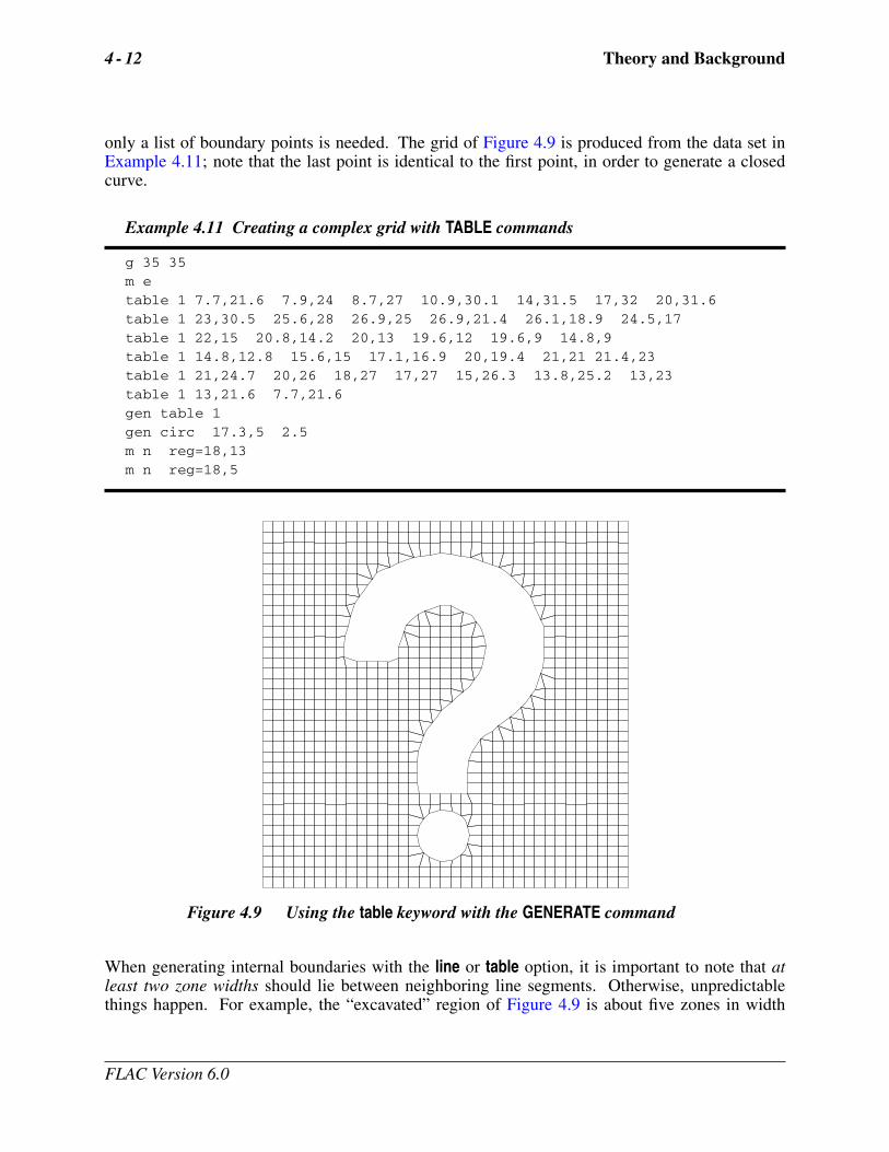
only a list of boundary points is needed. The grid of Figure 4.9 is produced from the data set inExample 4.11; note that the last point is identical to the first point, in order to generate a closedcurve.

Example 4.11 Creating a complex grid with TABLE commands

g 35 35m etable 1 7.7,21.6 7.9,24 8.7,27 10.9,30.1 14,31.5 17,32 20,31.6table 1 23,30.5 25.6,28 26.9,25 26.9,21.4 26.1,18.9 24.5,17table 1 22,15 20.8,14.2 20,13 19.6,12 19.6,9 14.8,9table 1 14.8,12.8 15.6,15 17.1,16.9 20,19.4 21,21 21.4,23table 1 21,24.7 20,26 18,27 17,27 15,26.3 13.8,25.2 13,23table 1 13,21.6 7.7,21.6gen table 1gen circ 17.3,5 2.5m n reg=18,13m n reg=18,5

Figure 4.9 Using the table keyword with the GENERATE command

When generating internal boundaries with the line or table option, it is important to note that atleast two zone widths should lie between neighboring line segments. Otherwise, unpredictablethings happen. For example, the “excavated” region of Figure 4.9 is about five zones in width

FLAC Version 6.0


– the generation process is well-behaved. If it is necessary to have very thin gaps between linesof relocated gridpoints, then it is advisable to zone up this region by hand, and do the rest withseveral applications of the GENERATE command. There are some geometries that just cannot beconstructed with an array of quadrilaterals when the required detail is fine enough. The questionto be asked is “Is the detail really necessary to the overall problem?”

The automatic generation scheme is not foolproof: there are some circumstances in which theresulting grid is not what was intended. In general, the boundary generators should only be usedwhen many gridpoints lie along the desired boundary; the scheme is not appropriate for relocatingonly two or three gridpoints at a time. In this case, the points should be moved individually by usingINITIAL x, y commands, as described previously. Even when most of the gridpoints on a surface arerelocated satisfactorily by the automatic generator, the two endpoints may have to be adjusted “byhand” with the INITIAL command, especially if they lie on an outer boundary. This is the case inthe next section, which is concerned with accommodating interfaces in a grid.

FLAC Version 6.0


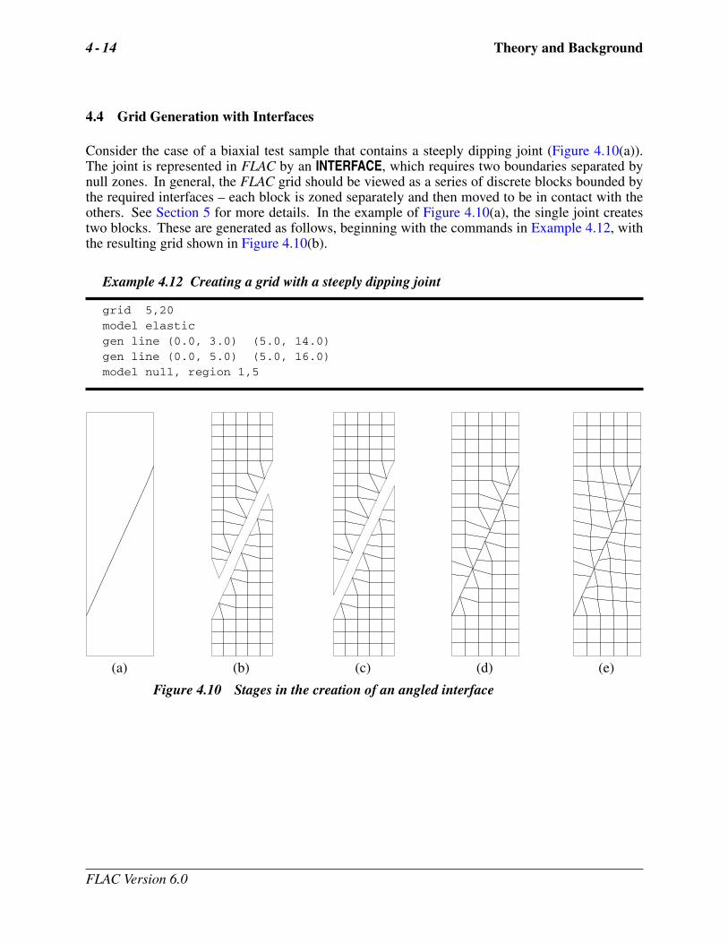
4.4 Grid Generation with Interfaces

Consider the case of a biaxial test sample that contains a steeply dipping joint (Figure 4.10(a)).The joint is represented in FLAC by an INTERFACE, which requires two boundaries separated bynull zones. In general, the FLAC grid should be viewed as a series of discrete blocks bounded bythe required interfaces – each block is zoned separately and then moved to be in contact with theothers. See Section 5 for more details. In the example of Figure 4.10(a), the single joint createstwo blocks. These are generated as follows, beginning with the commands in Example 4.12, withthe resulting grid shown in Figure 4.10(b).

Example 4.12 Creating a grid with a steeply dipping joint

grid 5,20model elasticgen line (0.0, 3.0) (5.0, 14.0)gen line (0.0, 5.0) (5.0, 16.0)model null, region 1,5

(a) (b) (c) (d) (e)

Figure 4.10 Stages in the creation of an angled interface

FLAC Version 6.0


The two badly placed endpoints can be moved, with the commands in Example 4.13, to producethe grid in Figure 4.10(c).

Example 4.13 Adjusting gridpoints along the joint

ini x=5.0 y=14.0 (i=6, j=14)ini x=0.0 y=5.0 (i=1, j=8)

Finally, the top block is moved down to meet the bottom block, and the two blocks are “joined” byan interface using the commands in Example 4.14 (see Figure 4.10(d)).

Example 4.14 Joining the two blocks

ini y (add) -2.0 i=1,2 j=8,21ini y (add) -2.0 i=3 j=10,21ini y (add) -2.0 i=4 j=13,21ini y (add) -2.0 i=5 j=15,21ini y (add) -2.0 i=6 j=16,21interface 1, ASIDE from 1,4 to 6,14 BSIDE from 1,8 to 6,17

The adjust operation is then applied to the central part of the interface example; the ends are leftalone by MARKing the appropriate gridpoints, using the commands in Example 4.15. (Recall thatmarked gridpoints are ignored by the GENERATE command.)

Example 4.15 Final adjustment to the grid

mark j=1,4mark j=17,21gen adjust

Figure 4.10(e) illustrates the result of this operation. When several interfaces are needed, thefollowing procedure should be followed. First, determine the number and shape of discrete blocksthat are bounded by the set of joints. Second, allocate part of the FLAC grid to each of the blocks,making sure that there is a buffer strip of at least one zone in width between blocks. Then, generatethe required geometry for each block separately. Finally, move the blocks together if this has notalready been done in the generation phase. This process is explained more fully in Section 5.3.

FLAC Version 6.0


4.5 Using Several Sub-Grids Attached Together

Quite complex shapes can be created by attaching several sub-grids together with the ATTACHcommand. Before attempting to do this, make a plan of the way the sub-grids are to be extractedfrom the initial grid provided by the GRID command. The procedure is like cutting rectangles ofpaper from a large sheet and then arranging them together in a different way. Each sub-grid must notshare gridpoints with any other sub-grid (i.e., there must be a “buffer region” at least one zone widebetween neighboring sub-grids). Once the sub-grids have been mapped out, they can be deformed,relocated and attached to other sub-grids.

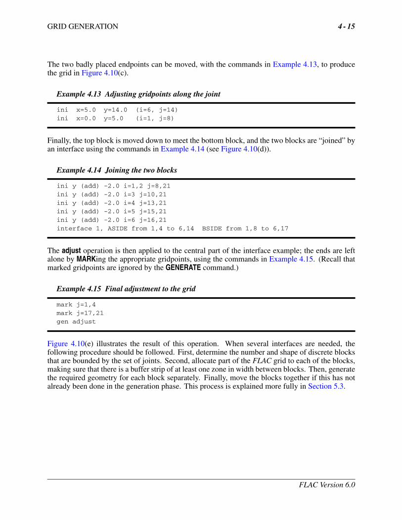
A good use of the ATTACH logic is to provide a well-graded boundary region around a finelyzoned central region of interest. The input sequence in Example 4.16 produces the grid shown inFigure 4.11.

Example 4.16 Creating a graded grid

grid 52,10model elas i=1,40 j=1,8model elas i=42,51 j=1,10gen 0,0 40,40 60,40 100,0 rat 1,0.83 i=1,11 j=1,9gen s s 60,60 100,100 rat 1,0.83 i=11,21 j=1,9gen s s 40,60 0,100 rat 1,0.83 i=21,31 j=1,9gen s s 40,40 0,0 rat 1,0.83 i=31,41 j=1,9attach aside from 1,1 to 1,9 bside from 41,1 to 41,9gen 40,40 40,60 60,60 60,40 i=42,52 j=1,11attach aside from 1,9 to 11,9 bside from 42,1 to 52,1attach aside from 12,9 to 41,9 bside (long) from 52,2 to 42,1

Figure 4.11 Graded grid produced with the ATTACH command

In this case, a 40 × 80 strip of zones is wrapped around the central region by means of fourGENERATE commands. The “tail” of the strip is then attached to the “head.” The strip is alsoattached to the central block at all points on the inner surface of the strip.

FLAC Version 6.0


Two sub-grids may be attached together even if the number of gridpoints on the opposing boundarypaths are not equal. However, the number of segments on one side must be an integral multipleof the number of segments on the other. The term “segment” here denotes the chord joining twoadjacent gridpoints on a boundary. For example, there may be 3 segments (4 gridpoints) on thefirst side and 6 segments (7 gridpoints) on the second side. In this case, the first, third, fifth andseventh gridpoints on the second side will be attached perfectly to their counterparts on the firstside. The remaining gridpoints on the second side are “slaved” to the two nearest perfectly attachedgridpoints on the same boundary, using linear weighting for forces and velocities. In the generalcase, every Nth gridpoint is attached perfectly to its opposing counterpart, where N is the integralratio of segments between the two sides.

Two boundaries may be attached in this way even if the opposing gridpoints are not at the samelocation, but a warning message will be issued for each pair that does not coincide. In this case, theslaved gridpoints still function as described above, but the weighting factors will be derived fromthe slave’s projection onto the chord joining the two nearest perfectly attached gridpoints. Greatcare should be taken when setting up attached boundaries in which the gridpoint spacing varies;a plot or printout should always be made to verify that the attachment has been done as intended.The command PRINT attach lists both perfectly attached groups and slaved gridpoints. The PLOTattach command only indicates perfectly attached gridpoints.

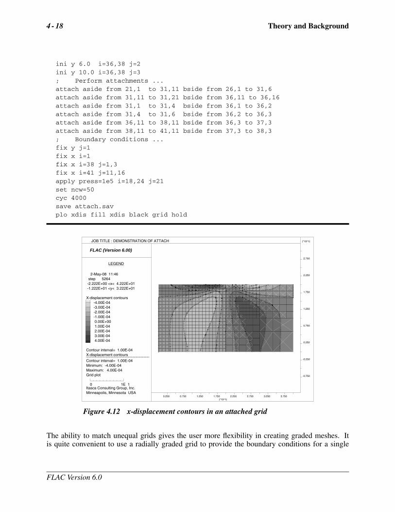
Example 4.17 illustrates the use of the ATTACH command when joining boundary paths with unequalnumbers of gridpoints. The example is unrealistic, but it serves to illustrate how a complicated seriesof connections can be made. In particular, the attachment of the lower, right-hand sub-grid illustratesthat two or more ATTACH commands may be needed if the integral ratio varies along a boundarypath that is to be attached. In this case, part of the boundary has a two-to-one ratio and the remainderhas a three-to-one ratio. Thus, two ATTACH commands are needed, even though the two opposingsub-grid boundaries are contiguous. After stepping, the results exhibit reasonable symmetry (seeFigure 4.12), which illustrates that coarse grids are adequate for regions that are remote from strainconcentrations.

Example 4.17 Demonstration of generalized ATTACH

; Note that the example is contrived, for illustration onlygrid 40,20model elas i=1,20 j=1,20 ; Create large regionmodel elas i=21,30 j=11,20model elas i=26,30 j=1,5 ; Create 1st medium-size regionmodel elas i=36,40 j=11,15 ; Create 2nd medium-size regionmodel elas i=36,37 j=1,2 ; Create small regionprop dens 2000 shear 1e8 bulk 2e8 ; (disregard warning messages!); Move regions to correct places ...ini x mul 2 y mul 2 x add -30 i=26,31 j=1,6ini x mul 2 y mul 2 x add -40 y add -10 i=36,41 j=11,16ini x 30.0 i=36 j=1,3ini x 34.0 i=37 j=1,3ini x 40.0 i=38 j=1,3

FLAC Version 6.0


ini y 6.0 i=36,38 j=2ini y 10.0 i=36,38 j=3; Perform attachments ...attach aside from 21,1 to 31,11 bside from 26,1 to 31,6attach aside from 31,11 to 31,21 bside from 36,11 to 36,16attach aside from 31,1 to 31,4 bside from 36,1 to 36,2attach aside from 31,4 to 31,6 bside from 36,2 to 36,3attach aside from 36,11 to 38,11 bside from 36,3 to 37,3attach aside from 38,11 to 41,11 bside from 37,3 to 38,3; Boundary conditions ...fix y j=1fix x i=1fix x i=38 j=1,3fix x i=41 j=11,16apply press=1e5 i=18,24 j=21set ncw=50cyc 4000save attach.savplo xdis fill xdis black grid hold

FLAC (Version 6.00)

LEGEND

2-May-08 11:46 step 5264 -2.222E+00 <x< 4.222E+01 -1.222E+01 <y< 3.222E+01

X-displacement contours -4.00E-04 -3.00E-04 -2.00E-04 -1.00E-04 0.00E+00 1.00E-04 2.00E-04 3.00E-04 4.00E-04

Contour interval= 1.00E-04X-displacement contours

Contour interval= 1.00E-04Minimum: -4.00E-04Maximum: 4.00E-04Grid plot

0 1E 1

-0.750

-0.250

0.250

0.750

1.250

1.750

2.250

2.750

(*10^1)

0.250 0.750 1.250 1.750 2.250 2.750 3.250 3.750(*10^1)

JOB TITLE : DEMONSTRATION OF ATTACH

Itasca Consulting Group, Inc. Minneapolis, Minnesota USA

Figure 4.12 x-displacement contours in an attached grid

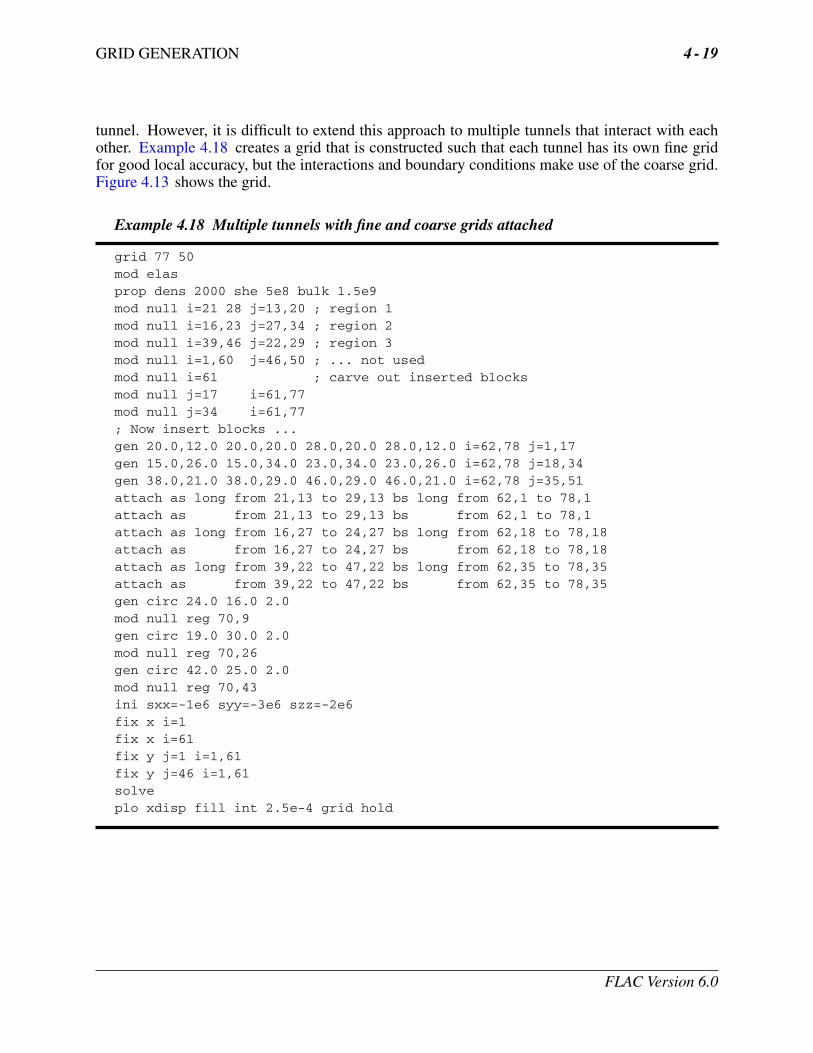
The ability to match unequal grids gives the user more flexibility in creating graded meshes. Itis quite convenient to use a radially graded grid to provide the boundary conditions for a single

FLAC Version 6.0


tunnel. However, it is difficult to extend this approach to multiple tunnels that interact with eachother. Example 4.18 creates a grid that is constructed such that each tunnel has its own fine gridfor good local accuracy, but the interactions and boundary conditions make use of the coarse grid.Figure 4.13 shows the grid.

Example 4.18 Multiple tunnels with fine and coarse grids attached

grid 77 50mod elasprop dens 2000 she 5e8 bulk 1.5e9mod null i=21 28 j=13,20 ; region 1mod null i=16,23 j=27,34 ; region 2mod null i=39,46 j=22,29 ; region 3mod null i=1,60 j=46,50 ; ... not usedmod null i=61 ; carve out inserted blocksmod null j=17 i=61,77mod null j=34 i=61,77; Now insert blocks ...gen 20.0,12.0 20.0,20.0 28.0,20.0 28.0,12.0 i=62,78 j=1,17gen 15.0,26.0 15.0,34.0 23.0,34.0 23.0,26.0 i=62,78 j=18,34gen 38.0,21.0 38.0,29.0 46.0,29.0 46.0,21.0 i=62,78 j=35,51attach as long from 21,13 to 29,13 bs long from 62,1 to 78,1attach as from 21,13 to 29,13 bs from 62,1 to 78,1attach as long from 16,27 to 24,27 bs long from 62,18 to 78,18attach as from 16,27 to 24,27 bs from 62,18 to 78,18attach as long from 39,22 to 47,22 bs long from 62,35 to 78,35attach as from 39,22 to 47,22 bs from 62,35 to 78,35gen circ 24.0 16.0 2.0mod null reg 70,9gen circ 19.0 30.0 2.0mod null reg 70,26gen circ 42.0 25.0 2.0mod null reg 70,43ini sxx=-1e6 syy=-3e6 szz=-2e6fix x i=1fix x i=61fix y j=1 i=1,61fix y j=46 i=1,61solveplo xdisp fill int 2.5e-4 grid hold

FLAC Version 6.0


FLAC (Version 6.00)

LEGEND

2-May-08 11:46 step 1556 -3.333E+00 <x< 6.333E+01 -1.083E+01 <y< 5.583E+01

Grid plot

0 2E 1

-0.500

0.500

1.500

2.500

3.500

4.500

(*10^1)

0.500 1.500 2.500 3.500 4.500 5.500(*10^1)

JOB TITLE : MULTIPLE TUNNELS WITH FINE AND COARSE GRIDS ATTACHED


Figure 4.13 Multiple tunnels with fine and coarse grids attached

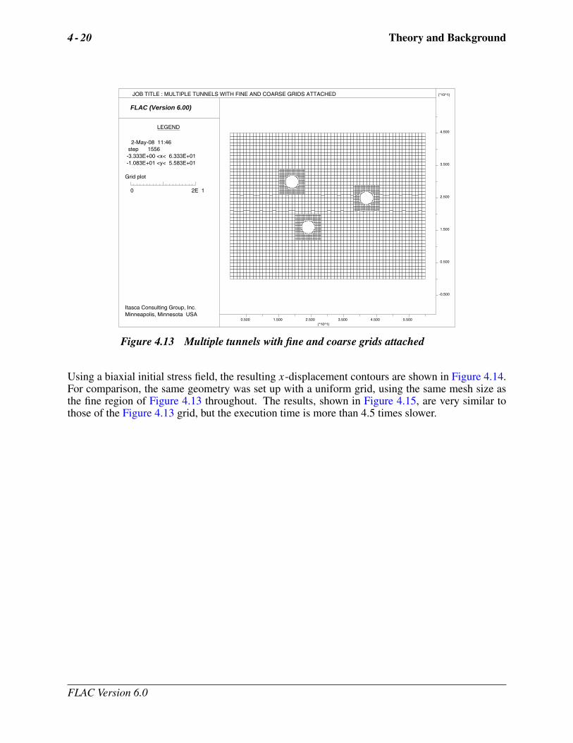
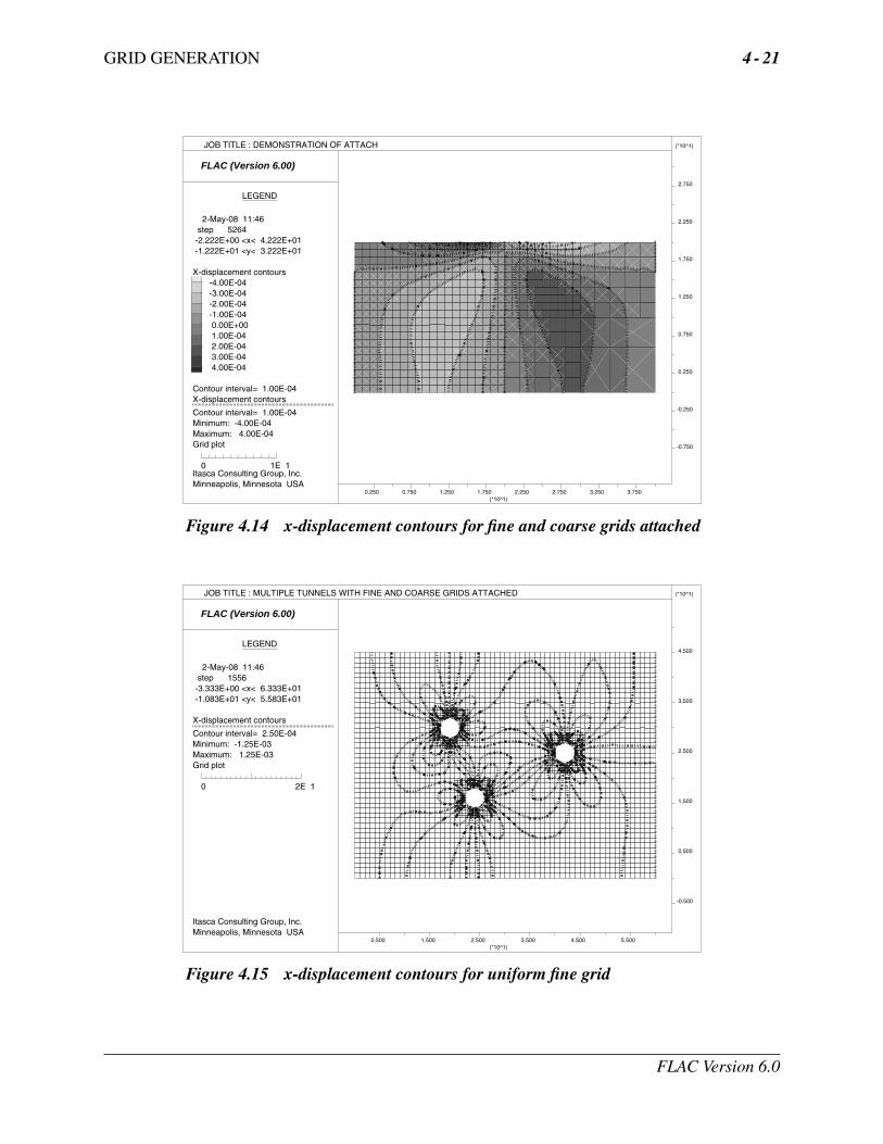
Using a biaxial initial stress field, the resulting x-displacement contours are shown in Figure 4.14.For comparison, the same geometry was set up with a uniform grid, using the same mesh size asthe fine region of Figure 4.13 throughout. The results, shown in Figure 4.15, are very similar tothose of the Figure 4.13 grid, but the execution time is more than 4.5 times slower.

FLAC Version 6.0


FLAC (Version 6.00)

LEGEND

2-May-08 11:46 step 5264 -2.222E+00 <x< 4.222E+01 -1.222E+01 <y< 3.222E+01

X-displacement contours -4.00E-04 -3.00E-04 -2.00E-04 -1.00E-04 0.00E+00 1.00E-04 2.00E-04 3.00E-04 4.00E-04

Contour interval= 1.00E-04X-displacement contours


0 1E 1

-0.750

-0.250

0.250

0.750

1.250

1.750

2.250

2.750

(*10^1)

0.250 0.750 1.250 1.750 2.250 2.750 3.250 3.750(*10^1)

JOB TITLE : DEMONSTRATION OF ATTACH


Figure 4.14 x-displacement contours for fine and coarse grids attached

FLAC (Version 6.00)

LEGEND

2-May-08 11:46 step 1556 -3.333E+00 <x< 6.333E+01 -1.083E+01 <y< 5.583E+01

X-displacement contours


0 2E 1

-0.500

0.500

1.500

2.500

3.500

4.500

(*10^1)

0.500 1.500 2.500 3.500 4.500 5.500(*10^1)

JOB TITLE : MULTIPLE TUNNELS WITH FINE AND COARSE GRIDS ATTACHED


Figure 4.15 x-displacement contours for uniform fine grid

FLAC Version 6.0


It is not meaningful to apply velocity boundary conditions or fix conditions to slaved gridpoints,because such gridpoints are controlled by their nearest attached neighbors. However, forces maybe applied to slaved gridpoints.

If all zones surrounding an attached gridpoint (slaved or not) are set to the null model, the attachcondition will still persist, even though such gridpoints will not participate in calculations. However,if real models are restored to the null zones, the previous attach conditions will be reactivated. Thereis no way to “unattach” gridpoints.

FLAC Version 6.0


4.6 Special-Purpose Grid Generation

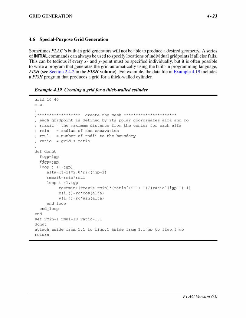
Sometimes FLAC ’s built-in grid generators will not be able to produce a desired geometry. A seriesof INITIAL commands can always be used to specify locations of individual gridpoints if all else fails.This can be tedious if every x- and y-point must be specified individually, but it is often possibleto write a program that generates the grid automatically using the built-in programming language,FISH (see Section 2.4.2 in the FISH volume). For example, the data file in Example 4.19 includesa FISH program that produces a grid for a thick-walled cylinder.

Example 4.19 Creating a grid for a thick-walled cylinder

grid 10 40m e;;****************** create the mesh **********************; each gridpoint is defined by its polar coordinates alfa and ro; rmaxit = the maximum distance from the center for each alfa; rmin = radius of the excavation; rmul = number of radii to the boundary; ratio = grid’s ratio;def donut

figp=igpfjgp=jgploop j (1,jgp)

alfa=(j-1)*2.0*pi/(jgp-1)rmaxit=rmin*rmulloop i (1,igp)

ro=rmin+(rmaxit-rmin)*(ratioˆ(i-1)-1)/(ratioˆ(igp-1)-1)x(i,j)=ro*cos(alfa)y(i,j)=ro*sin(alfa)

end_loopend_loop

endset rmin=1 rmul=10 ratio=1.1donutattach aside from 1,1 to figp,1 bside from 1,fjgp to figp,fjgpreturn

FLAC Version 6.0


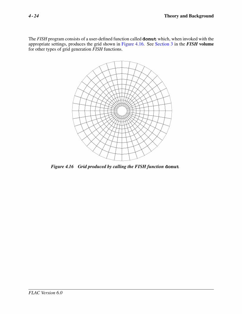
The FISH program consists of a user-defined function called donutwhich, when invoked with theappropriate settings, produces the grid shown in Figure 4.16. See Section 3 in the FISH volumefor other types of grid generation FISH functions.

Figure 4.16 Grid produced by calling the FISH function donut

FLAC Version 6.0

4 grid generation - missouri s&tweb.mst.edu/~norbert/ge5471/assignments/assign 1 - flac...

Documents