4.2 drawbacks of round robin scheduling...
TRANSCRIPT

Proposed Algorithm 1
The performance of the Round Robin Scheduling Algorithm relies on the size of the time
quantum. At one extreme, if the time quantum is extremely large, cause less response
time and it is similar to FCFS. If the time quantum is extremely small this causes too
many context switches and lowers the CPU efficiency. In this research I present a
solution to the disadvantages of Round Robin Scheduling Algorithm by make the
operating systems adjusting the process according to the burst time of the prevailed set of
processes in the FIFO queue based on priority.
Figure 4-1 Round Robin Processing
4.2 Drawbacks of Round Robin Scheduling Algorithm
Round Robin Scheduling Algorithm has many disadvantages are as following:
A. Higher Average Waiting Time

Proposed Algorithm 2
In round robin architecture the process spends the time in the ready queue for the waiting
of processor for implementation is known as waiting time and the time the process
completes. So, completing the process Round Robin Scheduling Algorithm produces
higher average waiting time which is the main disadvantage.
B. Low Throughput
Throughput is explained as number of process completed per time unit. If round robin is
executed in circular way then more context switches occur so throughput will be low
which leads to overall degradation of system performance. If the various context switches
is low then the throughput will be high. Context switch and throughput are inversely
proportional to each other.
C. Context Switch
When the time slice of the task finishes and the task is still executing on the processor the
scheduler forcibly preempts the tasks on the processor and stores the task context in stack
or registers and allots the processor to the next task in the ready queue. First of all the
processor save the state of process and implements next running process. When process
implement completely the processor continue execution of resumed process. This action
which is performed by the scheduler is known as context switch. Context switch leads to
the wastage of time, memory and leads to scheduler overhead.
D. High Response Time
Response time is the time from the submission of a request to the processor until the first
response is made that means when the task is submitted until the first response is
received. In general the round robin made larger response time which is the drawback
because system performance will be degraded. For the achieving high performance the
response time will be small.
E. Very High Turnaround Time
Turnaround time mentions to the total time between submission of a process and its
completion Round Robin scheduling algorithm also makes higher turnaround time which
is also drawback. For improving system performance we attaines lower turnaround time.

Proposed Algorithm 3
4.3 Adaptive Round Robin Scheduling Algorithms
4.3.1 Introduction to Adaptive RR
The Adaptive Round Robin (ARR) Scheduling Algorithm focuses on the demerits of
Simple Round Robin Algorithm which gives equal portion of time to all the processes
(processes are scheduled in first come first serve manner) because of all the demerits in
round robin algorithm is not efficient for processes with smaller CPU burst. This result
shows to the increase in waiting time and response time of processes which decrease the
system throughput. The Adaptive RR algorithm suspends the drawbacks of a simple
round robin algorithm in by scheduling of processes based on the CPU execution time.
The allotted processor used to reduce the burden of the main processor is assigned
processes according to the priority basis; the smaller CPU burst of the process, higher the
priority. The Adaptive RR Scheduling Algorithm resolves the problem of higher average
waiting time, turnaround time, and more context switches thereby improving the system
performance. The throughput mainly relies on the number of context switches; if context
switches decreased then throughput automatically improve.
4.3.2 Smart Time Slice for Adaptive RR
The Adaptive RR algorithm suspends the defects of Simple Round Robin (RR)
Scheduling Algorithm in Operating System by introducing a concept known as smart
time slice which depends on three aspects they are priority, average CPU burst or mid
process CPU burst, and context switch avoidance time. The Adaptive RR Scheduling
algorithm permits the user is to assign priority to the system based on execution time or
burst time. The calculated smart time slice will be founded on all CPU burst of new
running processes. The smart time slice calculated according to the processes burst time;
if the number of process are allotted into the ready queue are in odd manner the smart
time slice will be the mid process burst time else the number of processes are even in
ready queue the smart time slice is average of all processes burst time is allotted to the
processes.
Smart Time Slice = Mid Process Burst Time (If number of processes are odd

Proposed Algorithm 4
OR
Smart Time Slice = Average Burst Time (If number of processes are even)
Then processes are implementing according to the smart time slice and give superior
result comparison to existing Simple Round Robin Scheduling Algorithm and can be
executed in operating system.
Figure 4-2 Adaptive RR Architecture
4.4 Adaptive RR Pseudo Code
1. First of all examine ready queue is empty
2. When ready queue is vacant then all the processes are assigned into the ready
queue.
3. All the processes are sorted in increasing order that means smaller burst time
process get higher priority and larger burst time process get lower priority.
4. While (ready queue!= NULL)
5. Compute Smart Time Slice:
If (Number of process%2= = 0)
STS = average CPU burst time of all processes
Else

Proposed Algorithm 5
STS = mid process burst time
6. Allocate smart time slice to the ith process:
Pi STS
i=i+1
7. If ( i< Number of process) then go to step 6.
8. If a new process is arrived modernize the ready queue, go to step 2.
9. End of While
10. Compute average waiting time, turnaround time, context switches.
11. End

Proposed Algorithm 6
4.4.1 Flowchart for Adaptive RR
Figure 4-3 Flowchart for Adaptive Round Robin
4.4.2 Practical Implementation
Assumptions

Proposed Algorithm 7
1. The system should be unprocessed
2. The numbers of processes are unconventional
3. Smart Time Slice is deliberated form the number of processes and their burst time.
All the parameters like number of processes, their respective burst time and
arrival time should be priori known
4. All the processes are CPU bound
5. No Processes are I/O bound
4.4.3 Experimental work
Adaptive RR Algorithm consists of several input and output parameters like:
Input parameters
1. Number of process
2. CPU burst time
3. Arrival Time
4. Smart Time Slice
5. Priority
Output Parameters
1. Average Waiting Time
2. Average Turnaround Time
3. Number of context switches
4.4.4 Performance Metrics
1. Average Waiting Time: For better presentation on proposed algorithm, the
average waiting time should be small comparison to simple RR.

Proposed Algorithm 8
2. Average Turnaround Time: For better presentation on proposed algorithm, the
average turnaround time should be small comparison to simple RR.
3. Context Switches: For good presentation on proposed algorithm, the number of
context switches should be minimum comparison to simple RR.
4.4.5 Data Set
1. In first three cases I am appraising the data sets as the odd number of processes
with burst time in increasing, decreasing and random order. The arrival time for
every processes is zero.
2. Again in next three cases comprising even number of processes with burst time in
increasing, decreasing and random order. The arrival time for all processes is zero.
4.4.6 Research Practice with Expected Outcomes
To assess the performance of Adaptive RR algorithm, we have taken a set of processes in
different cases. Here for simplicity, we have taken 5 or 4 processes. The algorithm
performs effectively even if it used with a very large number of processes. In each case,
we have contrasted the experimental results of Adaptive algorithm with the Simple
Round Robin Scheduling Algorithm with fixed time quantum Q. Here we have supposed
a constant time quantum Q for simple RR and compare with Adaptive RR. In our
calculation I have varied the smart time slice which is rely on the number of processes.
The smart time slice can be calculated according to proposed plan.
Case 1:
We sort five processes arriving at time = 0, with increasing burst time (P1 = 10, P2 =20,
P3 = 30, P4 = 40, P5= 50) with time quantum =10 as shown in Table 4.1. The Table 4.2
shows the output using RR algorithm and Adaptive RR algorithm. Figure 4.4 and Figure
4.5 shows Gantt chart for both the algorithms simple RR and Adaptive RR respectively.
Table 4-1 Example of RR and ARR
Process Arrival Time (ms) Burst Time (ms)
P1 0 10

Proposed Algorithm 9
P2 0 20
P3 0 30
P4 0 40
P5 0 50
0 10 20 30 40 50 60 70 80 90 100 111 120 130 140 150
Figure 4-4 Gantt chart for Simple RR
Number of Context Switches = 14
Waiting time of P1 = 0
Waiting time of P2 = 40
Waiting time of P3 = 70
Waiting time of P4 = 90
Waiting time of P5 = 100
Average Waiting Time = [(P1+P2+P3+P4+P5)]/5
= (0+40+70+90+100)/5
= 300/5
= 60 ms
Turnaround Time for P1 = 10
Turnaround Time for P2 = 60
Turnaround Time for P3 = 100
Turnaround Time for P4 = 130
P
1
P
2
P
3P4
P
5
P
2
P
3
P
4
P
5P3
P
4
P
5
P
4
P
5P5

Proposed Algorithm 10
Turnaround Time for P5 = 150
Average Turnaround Time = [(P1+P2+P3+P4+P5)]/5
= (10+60+100+130+150)/5
= 450/5
= 90 ms
According to our proposed Algorithm
First of all we sort the processes in ready queue according their given burst time in
increasing order that is P1=10, P2=20, P3=30, P4=40 and P5=50 and after that we choose
the time quantum according Adaptive RR algorithm, the time quantum is the mid process
burst time if the given processes are odd, that is 30.The Gantt chart for Adaptive RR
P1 P2 P3 P4 P5 P4 P5
0 10 30 60 90 120 130 150
Figure 4-5 Gantt chart for Adaptive RR
Number of Context Switches = 6
Waiting time of P1 = 0
Waiting time of P2 = 10
Waiting time of P3 = 30
Waiting time of P4 = 90
Waiting time of P5 = 100
Average Waiting Time = [(P1+P2+P3+P4+P5)]/5
= (0+10+30+90+100)/5
= 230/5 ms
= 46 ms

Proposed Algorithm 11
Turnaround Time for P1 = 10
Turnaround Time for P2 = 30
Turnaround Time for P3 = 60
Turnaround Time for P4 = 130
Turnaround Time for P5 = 150
Average Turnaround Time = (P1+P2+P3+P4+P5)/5
= (10+30+60+130+150)/5
= 380/5
= 76 m
Table 4-2 Comparison of Simple RR and Adaptive RR
Algorithm
Time
Quantu
m
C
S
Average
WT
Average
TAT
Through
Put
Simple RR 10 14 60 90 Low
Adaptive RR 45 6 46 76High
Case 2:
We suppose five processes arriving at time = 0, with increasing burst time (P1 =13, P2
=35, P3 = 46, P4 = 63, P5= 97) with time quantum = 25 as shown in Table 4.3. The Table
4.4 shows the output using RR algorithm and Adaptive RR algorithm. Figure4.6 and
Figure 4.7 shows Gantt chart for both the algorithms respectively.
Table 4-3 Example 2 of RR and ARR
Process Arrival Time (ms) Burst Time (ms)
P1 0 13
P2 0 35

Proposed Algorithm 12
P3 0 46
P4 0 63
P5 0 97
P1 P2 P3 P4 P5 P2 P3 P4 P5 P4 P5 P5
0 13 38 63 88 113 123 144 169 194 207 232 254
Figure 4-6 Gantt chart for simple RR
Number of context switches = 11
Waiting time of P1 = 0
Waiting time of P2 = 88
Waiting time of P3 = 98
Waiting time of P4 = 144
Waiting time of P5 = 157
Average Waiting Time = [(P1+P2+P3+P4+P5)]/5
= [(0+88+98+144+157)]/5
= (487)/5
= 97.4 ms
Turnaround Time for P1 = 13
Turnaround Time for P2 = 123
Turnaround Time for P3 = 144
Turnaround Time for P4 = 207
Turnaround Time for P5 = 254
Average Turnaround Time = [(P1+P2+P3+P4+P5)]/5
= [(13+123+144+232+304)]/5
= 741/5
= 148.2 ms
According our proposed mechanism

Proposed Algorithm 13
First of all we sort the processes in ready queue according their given burst time in
increasing order that is P1 =13, P2 =35, P3 = 46, P4 = 63, P5= 97and after that we choose
the time quantum according Adaptive RR algorithm, the time quantum is the mid process
burst time if the given processes are odd, that is 46.The Gantt chart for Adaptive RR
P1 P2 P3 P4 P5 P4 P5 P5
0 13 48 94 140 186 203 249 254
Figure 4-6 Gantt chart for Adaptive RR
Number of context switches =7
Waiting time of P1 = 0
Waiting time of P2 = 13
Waiting time of P3 = 48
Waiting time of P4 = 140
Waiting time of P5 = 157
Average Waiting Time = [(P1+P2+P3+P4+P5)]/5
= [(0+13+48+140+157)]/5
= (358)/5
= 71.6 ms
Turnaround Time for P1 = 13
Turnaround Time for P2 = 48
Turnaround Time for P3 = 94
Turnaround Time for P4 = 203
Turnaround Time for P5 = 254
Average Turnaround Time = [(P1+P2+P3+P4+P5)]/5
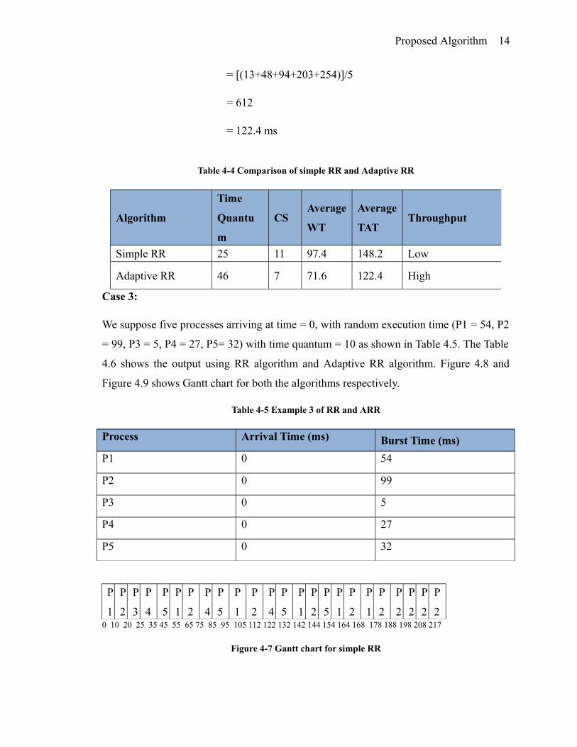
Proposed Algorithm 14
= [(13+48+94+203+254)]/5
= 612
= 122.4 ms
Table 4-4 Comparison of simple RR and Adaptive RR
Case 3:
We suppose five processes arriving at time = 0, with random execution time (P1 = 54, P2
= 99, P3 = 5, P4 = 27, P5= 32) with time quantum = 10 as shown in Table 4.5. The Table
4.6 shows the output using RR algorithm and Adaptive RR algorithm. Figure 4.8 and
Figure 4.9 shows Gantt chart for both the algorithms respectively.
Table 4-5 Example 3 of RR and ARR
Process Arrival Time (ms) Burst Time (ms)
P1 0 54
P2 0 99
P3 0 5
P4 0 27
P5 0 32
P
1
P
2
P
3
P
4
P
5
P
1
P
2
P
4
P
5
P
1
P
2
P
4
P
5
P
1
P
2
P
5
P
1
P
2
P
1
P
2
P
2
P
2
P
2
P
20 10 20 25 35 45 55 65 75 85 95 105 112 122 132 142 144 154 164 168 178 188 198 208 217
Figure 4-7 Gantt chart for simple RR
Algorithm
Time
Quantu
m
CSAverage
WT
Average
TATThroughput
Simple RR 25 11 97.4 148.2 Low
Adaptive RR 46 7 71.6 122.4 High

Proposed Algorithm 15
Number of context switches = 23
Waiting time of P1 = 114
Waiting time of P2 = 118
Waiting time of P3 = 20
Waiting time of P4 = 85
Waiting time of P5 = 112
Average Waiting Time = [(P1+P2+P3+P4+P5)]/5
= [(114+118+20+85+112)]/5
= (449)/5
= 89.8 ms
Turnaround Time for P1 = 168
Turnaround Time for P2 = 217
Turnaround Time for P3 = 25
Turnaround Time for P4 = 112
Turnaround Time for P5 = 144
Average Turnaround Time = [(P1+P2+P3+P4+P5)]/5
= [(168+217+25+122+144)]/5
= 666
= 133.2 ms
According our proposed mechanism
First of all we sort the processes in ready queue according their given burst time in
increasing order that is P3=5, P4= 27, P5=32, P1=54 and P2=99 and after that we choose
the time quantum according Adaptive RR algorithm, the time quantum is the mid process
burst time if the given processes are odd, that is 32.The Gantt chart for Adaptive RR
P3 P4 P5 P1 P2 P1 P2 P2 P2
0 5 32 64 96 128 150 182 214 217
Figure 4-8 Gantt chart for Adaptive RR
Number of context switches = 8

Proposed Algorithm 16
Waiting time of P1 = 96
Waiting time of P2 = 118
Waiting time of P3 = 0
Waiting time of P4 = 5
Waiting time of P5 = 32
Average Waiting Time = [(P1+P2+P3+P4+P5)]/5
= [(96+118+0+5+32)]/5
= 251
= 50.2 ms
Turnaround Time for P1 = 150
Turnaround Time for P2 = 217
Turnaround Time for P3 = 5
Turnaround Time for P4 = 32
Turnaround Time for P5 = 64
Average Turnaround Time = [(P1+P2+P3+P4+P5)]/5
= [(150+217+5+32+64)]/5
= 93.6 ms
Table 4-6 Comparison of simple RR and Adaptive RR
AlgorithmTime
QuantumCS Average WT Average TAT Throughput
Simple RR 26 23 89.8 133.2 Low
Adaptive
RR35 8 50.2 93.6 High

Proposed Algorithm 17
Case 4:
We suppose five processes arriving at time = 0, with increasing burst time (P1 = 14, P2
=34, P3 = 45, P4 = 62, P5= 77) with time quantum =25 as shown in Table 4.7. The Table
4.8 shows the output using RR algorithm and Adaptive RR algorithm. Figure 4.10 and
Figure 4.11 shows Gantt chart for both the algorithms simple RR and Adaptive RR
respectively.
Table 4-7 Example 1of RR and ARR
Process Arrival Time (ms) Burst Time (ms)
P1 0 14
P2 0 34
P3 0 45
P4 0 62
P5 0 77
P1 P2 P3 P4 P5 P2 P3 P4 P5 P4 P5 P5
0 14 39 64 89 114 123 143 168 193 205 230 232
Figure 4-9 Gantt chart for Simple RR
Number of Context Switches = 11
Waiting time of P1 = 0
Waiting time of P2 = 89
Waiting time of P3 = 98
Waiting time of P4 = 143
Waiting time of P5 = 155
Average Waiting Time = [(P1+P2+P3+P4+P5)]/5
= (0+89+98+143+155)/5
= 486/5
= 97 ms

Proposed Algorithm 18
Turnaround Time for P1 = 14
Turnaround Time for P2 = 123
Turnaround Time for P3 = 143
Turnaround Time for P4 = 205
Turnaround Time for P5 = 232
Average Turnaround Time = [(P1+P2+P3+P4+P5)]/5
= (14+123+143+205+232)/5
= 717/5
= 143.4 ms
According our proposed mechanism
First of all we sort the processes in ready queue according their given burst time in
increasing order that is P1=14, P2=34, P3=45, P4=62 and P5=77 and after that we choose
the time quantum according Adaptive RR algorithm, the time quantum is the mid process
burst time if the given processes are odd, that is 45.The Gantt chart for Adaptive RR
P1 P2 P3 P4 P5 P4 P5
0 14 48 93 138 183 200 232
Figure 4-10 Gantt chart for Adaptive RR
Number of Context Switches = 6
Waiting time of P1 = 0
Waiting time of P2 = 14
Waiting time of P3 = 48
Waiting time of P4 = 138
Waiting time of P5 = 155
Average Waiting Time = [(P1+P2+P3+P4+P5)]/5
= (0+14+48+138+155)/5
= 71 ms
Turnaround Time for P1 = 14
Turnaround Time for P2 = 48

Proposed Algorithm 19
Turnaround Time for P3 = 93
Turnaround Time for P4 = 200
Turnaround Time for P5 = 232
Average Turnaround Time = (P1+P2+P3+P4+P5)/5
= (14+48+93+200+232)/5
= 587/5
= 117.4 ms
Table 4-8 Comparison of Simple RR and Adaptive RR
AlgorithmTime
QuantumCS Average WT Average TAT Throughput
Simple RR 25 11 97 143.4 Low
Adaptive
RR45 6 71 117.4 High
Case 5:
We suppose five processes arriving at time = 0, with decreasing burst time (P1 = 83, P2
=54, P3 = 30, P4 = 19, P5= 8) with time quantum = 26 as shown in Table 4.9. The Table
4.10 shows the output using RR algorithm and Adaptive RR algorithm. Figure 4.12 and
Figure 4.13 shows Gantt chart for both the algorithms respectively.
Table 4-9 Example 2 of RR and ARR
Process Arrival Time (ms) Burst Time (ms)
P1 0 83
P2 0 54
P3 0 30
P4 0 19
P5 0 8
P1 P2 P3 P4 P5 P1 P2 P3 P1 P2 P1
0 26 52 78 97 105 131 157 161 187 189 194

Proposed Algorithm 20
Figure 4-11 Gantt chart for simple RR
Number of context switches = 10
Waiting time of P1 = 111
Waiting time of P2 = 135
Waiting time of P3 = 131
Waiting time of P4 = 78
Waiting time of P5 = 97
Average Waiting Time = [(P1+P2+P3+P4+P5)]/5
= [(111+135+131+78+97)]/5
= (552)/5
= 110.4 ms
Turnaround Time for P1 = 194
Turnaround Time for P2 = 189
Turnaround Time for P3 = 161
Turnaround Time for P4 = 97
Turnaround Time for P5 = 105
Average Turnaround Time = [(P1+P2+P3+P4+P5)]/5
= [(194+189+161+97+105)]/5
= 746/5
= 149.2 ms
According our proposed mechanism
First of all I sort the processes in ready queue according their given burst time in
increasing order that is P5=8, P4=19, P3=30, P2=54 and P5=83 and after that I choosing
the time quantum according Adaptive RR algorithm, the time quantum is the mid process
burst time if the given processes are odd, that is 30.The Gantt chart for Adaptive RR
P5 P4 P3 P2 P1 P2 P1 P1
0 8 27 57 87 117 141 171 194
Figure 4-12 Gantt chart for Adaptive RR
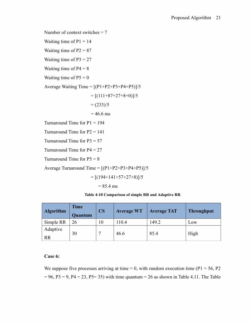
Proposed Algorithm 21
Number of context switches = 7
Waiting time of P1 = 14
Waiting time of P2 = 87
Waiting time of P3 = 27
Waiting time of P4 = 8
Waiting time of P5 = 0
Average Waiting Time = [(P1+P2+P3+P4+P5)]/5
= [(111+87+27+8+0)]/5
= (233)/5
= 46.6 ms
Turnaround Time for P1 = 194
Turnaround Time for P2 = 141
Turnaround Time for P3 = 57
Turnaround Time for P4 = 27
Turnaround Time for P5 = 8
Average Turnaround Time = [(P1+P2+P3+P4+P5)]/5
= [(194+141+57+27+8)]/5
= 85.4 ms
Table 4-10 Comparison of simple RR and Adaptive RR
AlgorithmTime
QuantumCS Average WT Average TAT Throughput
Simple RR 26 10 110.4 149.2 Low
Adaptive
RR30 7 46.6 85.4 High
Case 6:
We suppose five processes arriving at time = 0, with random execution time (P1 = 56, P2
= 96, P3 = 9, P4 = 23, P5= 35) with time quantum = 26 as shown in Table 4.11. The Table

Proposed Algorithm 22
4.12 shows the output using RR algorithm and Adaptive RR algorithm. Figure 4.14 and
Figure 4.15 shows Gantt chart for both the algorithms respectively.
Table 4-11 Example 6 of RR and ARR
Process Arrival Time (ms) Burst Time (ms)
P1 0 56
P2 0 96
P3 0 9
P4 0 23
P5 0 35
P1 P2 P3 P4 P5 P1 P2 P3 P1 P2 P20 26 52 61 84 110 136 162 171 175 201 219
Figure 4-13 Gantt chart for simple RR
Number of context switches = 10
Waiting time of P1 = 119
Waiting time of P2 = 123
Waiting time of P3 = 52
Waiting time of P4 = 61
Waiting time of P5 = 136
Average Waiting Time = [(P1+P2+P3+P4+P5)]/5
= [(119+123+52+61+136)]/5
= (491)/5
= 98.2 ms
Turnaround Time for P1 = 175
Turnaround Time for P2 = 219
Turnaround Time for P3 = 61
Turnaround Time for P4 = 84
Turnaround Time for P5 = 171

Proposed Algorithm 23
Average Turnaround Time = [(P1+P2+P3+P4+P5)]/5
= [(175+219+61+84+171)]/5
= 142 ms
According our proposed mechanism:
First of all we sort the processes in ready queue according their given burst time in
increasing order that is P3=9, P4= 23, P5=35, P1=56 and P2=96 and after that we select
the time quantum according Adaptive RR algorithm, the time quantum is the mid process
burst time if the given processes are odd, that is 35.The Gantt chart for Adaptive RR
P3 P4 P5 P1 P2 P1 P2 P2
0 9 32 67 102 137 158 193 219
Figure 4-14 Gantt chart for Adaptive RR
Number of context switches =7
Waiting time of P1 = 102
Waiting time of P2 = 123
Waiting time of P3 = 0
Waiting time of P4 = 9
Waiting time of P5 = 32
Average Waiting Time = [(P1+P2+P3+P4+P5)]/5
= [(102+123+0+9+32)]/5
= 53.2 ms
Turnaround Time for P1 = 158
Turnaround Time for P2 = 219
Turnaround Time for P3 = 9
Turnaround Time for P4 = 32
Turnaround Time for P5 = 67
Average Turnaround Time = [(P1+P2+P3+P4+P5)]/5
= [(158+219+9+32+67)]/5
= 97 ms

Proposed Algorithm 24
Table 4-12 Comparison of simple RR and Adaptive RR
AlgorithmTime
QuantumCS Average WT Average TAT Throughput
Simple RR 26 10 98.2 142 Low
Adaptive
RR35 7 53.2 97 High
Case 7:
We suppose four processes arriving at time = 0, with increasing burst time (P1 = 20, P2
=31, P3 = 43, P4 = 55) with time quantum =26 as shown in Table 4.13. The Table 4.14
shows the output using RR algorithm and Adaptive RR algorithm. Figure 4.16 and Figure
4.17 shows Gantt chart for both the algorithms respectively.
Table 4-13 Example 7 of RR and ARR
Process Arrival Time (ms) Burst Time (ms)
P1
P2
P3
P4
0
0
0
0
20
31
43
55
P1 P2 P3 P4 P2 P3 P4 P4
0 20 46 72 98 103 120 146 149
Figure 4-15 Gantt chart for Simple RR
Number of Context Switches = 6
Waiting time of P1 = 0
Waiting time of P2 = 72
Waiting time of P3 = 77
Waiting time of P4 = 94
Average Waiting Time = [(P1+P2+P3+P4)]/4

Proposed Algorithm 25
= (0+72+77+120)/4
= 243/4
= 60.75 ms
Turnaround Time for P1 = 20
Turnaround Time for P2 = 103
Turnaround Time for P3 = 120
Turnaround Time for P4 = 14
Average Turnaround Time = [(P1+P2+P3+P4)]/4
= (20+103+120+149)/4
= 392/4
= 98 ms
According Adaptive RR mechanism:
First of all we sort the processes in ready queue according their given burst time in
increasing order that is P1=20, P2=31, P3=43 and P4=55 and after that we choose the
time quantum according Adaptive RR Algorithm, the time quantum is the average
processes burst time if the given processes are even, that is 37.The Gantt chart for
Adaptive RR
P1 P2 P3 P4 P3 P4
0 20 51 88 125 131 149
Figure 4-16 Gantt chart for Adaptive RR
Number of Context Switches = 5
Waiting time of P1 = 0
Waiting time of P2 = 20
Waiting time of P3 = 88
Waiting time of P4 = 94
Average Waiting Time = [(P1+P2+P3+P4)]/4
= (0+20+88+94)/4
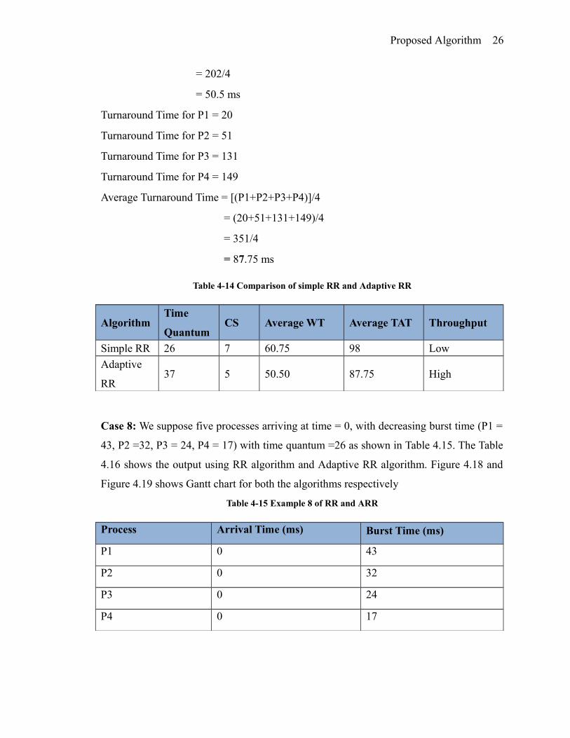
Proposed Algorithm 26
= 202/4
= 50.5 ms
Turnaround Time for P1 = 20
Turnaround Time for P2 = 51
Turnaround Time for P3 = 131
Turnaround Time for P4 = 149
Average Turnaround Time = [(P1+P2+P3+P4)]/4
= (20+51+131+149)/4
= 351/4
= 87.75 ms
Table 4-14 Comparison of simple RR and Adaptive RR
AlgorithmTime
QuantumCS Average WT Average TAT Throughput
Simple RR 26 7 60.75 98 Low
Adaptive
RR37 5 50.50 87.75 High
Case 8: We suppose five processes arriving at time = 0, with decreasing burst time (P1 =
43, P2 =32, P3 = 24, P4 = 17) with time quantum =26 as shown in Table 4.15. The Table
4.16 shows the output using RR algorithm and Adaptive RR algorithm. Figure 4.18 and
Figure 4.19 shows Gantt chart for both the algorithms respectively
Table 4-15 Example 8 of RR and ARR
Process Arrival Time (ms) Burst Time (ms)
P1 0 43
P2 0 32
P3 0 24
P4 0 17

Proposed Algorithm 27
P1 P2 P3 P4 P1 P2
0 26 52 76 93 110 116
Figure 4-17 Gantt chart for Simple RR
Number of Context Switches = 5
Waiting time of P1 = 67
Waiting time of P2 = 84
Waiting time of P3 = 52
Waiting time of P4 = 76
Average Waiting Time = [(P1+P2+P3+P4)]/4
= (67+84+52+76)/4
= 279/4
= 69.75 ms
Turnaround Time for P1 = 110
Turnaround Time for P2 = 116
Turnaround Time for P3 = 76
Turnaround Time for P4 = 93
Average Turnaround Time = [(P1+P2+P3+P4)]/4
= (110+116+76+93)/4
= 395/4
= 98.75 ms
According Adaptive RR mechanism:
First of all we sort the processes in ready queue according their given burst time in
increasing order that is P4=17, P3=24, P2=32 and P1=43 and after that we choose the
time quantum according Adaptive RR algorithm, the time quantum is the average
processes burst time if the given processes are even, that is 29.The Gantt chart for
Adaptive RR
P4 P3 P2 P1 P2 P1

Proposed Algorithm 28
0 17 41 70 99 102 116
Figure 4-18 Gantt chart for Adaptive RR
Number of Context Switches = 5
Waiting time of P1 = 73
Waiting time of P2 = 70
Waiting time of P3 = 17
Waiting time of P4 = 0
Average Waiting Time = [(P1+P2+P3+P4)]/4
= (73+70+17+0)/4
= 160/4
= 40 ms
Turnaround Time for P1 = 106
Turnaround Time for P2 = 102
Turnaround Time for P3 = 41
Turnaround Time for P4 = 17
Average Turnaround Time = [(P1+P2+P3+P4)]/4
= (106+102+41+17)/4
= 276/4
= 69 ms
Table 4-16 Comparison of simple RR and Adaptive RR
Algorith
m
Time
Quantum
CS Average WT Average TAT Throughput
Simple RR 26 5 69.75 98.75 Low
Adaptive
RR
29 5 40 69 High
Case 9:
We suppose four processes arriving at time = 0, with random burst time (P1 = 20, P2 =32,
P3 = 9, P4 = 19) with time quantum =16 as shown in Table 4.17. The Table 4.18 shows

Proposed Algorithm 29
the output using RR algorithm and Adaptive R algorithm. Figure 4.20 and Figure 4.21
shows Gantt chart for both the algorithms respectively.
Table 4-17 Example 6 of RR and ARR
Process Arrival Time (ms) Burst Time (ms)
P1 0 20
P2 0 32
P3 0 9
P4 0 19
P1 P2 P3 P4 P1 P2 P4
0 16 32 41 57 61 77 80
Figure 4-19 Gantt chart for Simple RR
Number of Context Switches = 6
Waiting time of P1 = 41
Waiting time of P2 = 45
Waiting time of P3 = 32
Waiting time of P4 = 61
Average Waiting Time = [(P1+P2+P3+P4)]/4
= (41+45+32+61)/4
= 179/4
= 44.75 ms
Turnaround Time for P1 = 61
Turnaround Time for P2 = 77
Turnaround Time for P3 = 41
Turnaround Time for P4 = 80
Average Turnaround Time = [(P1+P2+P3+P4)]/4
= (61+77+41+80)/4
= 259/4

Proposed Algorithm 30
= 64.75 ms
According Adaptive RR mechanism
First of all we order the processes in ready queue according their given burst time in
increasing order that is P3=9, P4=19, P1=20 and P2=32 and after that we choose the time
quantum according Adaptive RR algorithm, the time quantum is the average processes
burst time if the provided processes are even, that is 20.The Gantt chart for Adaptive RR
P3 P4 P1 P2 P2
0 9 28 48 68 80
Figure 4-20 Gantt chart for Adaptive RR
Number of Context Switches = 4
Waiting time of P1 = 28
Waiting time of P2 = 48
Waiting time of P3 = 0
Waiting time of P4 = 9
Average Waiting Time = [(P1+P2+P3+P4)]/4
= (28+48+0+9)/4
= 85/4
= 21.25 ms
Turnaround Time for P1 = 48
Turnaround Time for P2 = 80
Turnaround Time for P3 = 9
Turnaround Time for P4 = 28
Average Turnaround Time = [(P1+P2+P3+P4)]/4
= (48+80+9+0)/4
= 165/4

Proposed Algorithm 31
= 41.25 ms
Table 4-18 Comparison of simple RR and Adaptive RR
Algorith
m
Time
QuantumCS Average WT Average TAT Throughput
Simple RR 16 6 44.75 64.7 Low
Adaptive
RR20 3 21.25 41.25 High
Case 10:
We suppose five processes arriving at time = 0, with random burst time (P1 = 24, P2 =36,
P3 = 3, P4 = 3 and P5=10) with time quantum =4 as shown in Table 4.19. The Table 4.20
shows the output using RR algorithm and Adaptive RR algorithm. Figure 4.22 and Figure
4.23 shows Gantt chart for both the algorithms respectively.
Table 4-19 Example 10 of RR and ARR
Process Arrival Time (ms) Burst Time (ms)
P1 0 24
P2 0 36
P3 0 3
P4 0 3
P5 0 10
P
1
P
2
P
3
P
4
P
5
P
1
P
2
p
5
P
1
P
2
P
5
P
1
P2 P
1
P2 P1 P2 P2 P2 P
20 4 8 11 14 18 22 26 30 34 38 40 44 48 52 56 60 64 68 72 76
Figure 4-21 Gantt chart for Simple RR
Number of Context Switches = 19
Waiting time of P1 = 36
Waiting time of P2 = 40

Proposed Algorithm 32
Waiting time of P3 = 8
Waiting time of P4 = 11
Waiting time of P5 =30
Average Waiting Time = [(P1+P2+P3+P4+P5)]/5
= (36+40+8+11+30)/5
= 125/5
= 25 ms
Turnaround Time for P1 = 60
Turnaround Time for P2 = 76
Turnaround Time for P3 = 11
Turnaround Time for P4 = 14
Turnaround Time for P5 = 40
Average Turnaround Time = [(P1+P2+P3+P4+P5)]/5
= (60+76+11+14+40)/5
= 201/5
= 40.2 ms
According Adaptive RR mechanism:
First of all we order the processes in ready queue according their given burst time in
increasing order that is P3=3, P4=3, P5=10 ,P1=24and P2=36 and after that we selecting
the time quantum according Adaptive RR algorithm, the time quantum is the mid
processes burst time if the given processes are odd, that is 10.The Gantt chart for
Adaptive RR
P3 P4 P5 P1 P2 P1 P2 P1 P2 P2
0 3 6 16 26 36 46 56 60 70 76
Figure 4-22 Gantt chart for Adaptive RR
Number of Context Switches = 9
Waiting time of P1 = 36

Proposed Algorithm 33
Waiting time of P2 = 40
Waiting time of P3 = 0
Waiting time of P4 = 3
Waiting time of P5 = 6
Average Waiting Time = [(P1+P2+P3+P4+p5)]/5
= (36+40+0+3+6)/5
= 85/5
= 17 ms
Turnaround Time for P1 = 60
Turnaround Time for P2 = 76
Turnaround Time for P3 = 3
Turnaround Time for P4 = 6
Turnaround Time for P5 = 16
Average Turnaround Time = [(P1+P2+P3+P4+P5)]/5
= (60+76+3+6+16)/5
= 161/5
= 32.2 ms
Table 4-20 Comparison of simple RR and Adaptive RR
Algorith
m
Time
QuantumCS
Average
WTAverage TAT Throughput
Simple RR 4 19 25 40.2 Low
Adaptive
RR10 9 17 32.2 High