422 final project

Factors that Influence the U.S Imports of Goods from Japan

Fanyu Guo, Kaidi Meng and Dayi Fang

November 14, 2013

Abstract

The United States is the world’s largest importer that mainly imports industrial machinery and equipment, capital goods,

consumer goods and automotive supplies. Analyzing the factors related to the U.S. imports assists predicting the import

values for the next business cycle and helps solve the balance deficit problem. By reviewing literatures on exchange rate

effects on U.S imports, U.S.- Japan economic relations and how imports support U.S jobs gave us a general background

related to the factors that affecting the U.S. imports from Japan. We defined five variables in a time-series model and ran

a multiple regression to examine each variable’s significance. We used time series component such as the effects of

trends, seasonality, broken trend and cycles. In addition, we incorporated functional forms related to cycles, AR models,

ACFs/PACFs, and ADL models. Analyzing the factors that determines the United States’ imports in goods from Japan

could show a general idea of the complicated economic market. At last, we came up with a relatively good model to

predict future values for the U.S. imports of good from Japan.

KEY WORDS: U.S IMPORTS, JAPAN, EXCHANGE RATE, MUTIPLE REGRESSION,

PREDICT, TIME-SERIES MODEL

1

I. Introduction

United States is the world’s largest importer that mainly imports industrial machinery and

equipment (USD 731 billion), capital goods (USD 548 billion), consumer goods (USD 517 billion)

and automotive supplies (USD 297 billions)(US Economy). The U.S. Census Bureau reported that

from 1992 to 2013, the average of United States imports is 136,257.7 USD Million reaching an all

time high of 234,295.0 USD Million in March of 2012 and a record low of 52,277.0 USD Million in

January of 1992(Trading Economics 2013). Main imports countries are: China (18 percent of total

imports), European Union (16 percent), Canada (14 percent), Mexico (12 percent) and Japan (6

percent). Japanese Prime Minister Shinzo Abe’s “Abenomics” strategy made Japan’s currency

dropped below 90 Yen to USD to benefit Japan’s export-reliant economy.

In this research paper, we want to find out the factors that influence the United States

imports of good from Japan. Since U.S. has a huge value of imports, which may cause

unemployment, decrease in long-term trade competitiveness and lowers consumer confidence. Our

dependent variable is U.S. Imports of Goods from Japan (IMPJP), Customs Basis and our

independent variables are U.S. Imports of Goods from Canada, Customs Basis (IMPCA), U.S.

Imports of Goods from China, Mainland, Customs Basis (IMPCH), S&P 500 Stock Price Index

(SP500) and Japan / U.S. Foreign Exchange Rate (DEXJPUS). Furthermore, we introduce time

series component related to the effects of trends, seasonality, broken trend, cycles and lags, and with

the support of functional forms related to cycles, AR models, ACFs/ PACFs, and ADL models. In

our final regression model, we find that the U.S. imports of goods from Japan is affected by log of

the U.S. imports of goods from China, log of the U.S. imports of goods from Canada, and the

Exchange rate between U.S. dollars and Japanese. The U.S. balance of trade is facing a huge deficit

for more than 10 years and this number is rising annually. As a result, we come up with a relatively

good model for predicting future values for U.S. imports of goods from Japan. By analyzing these

2

factors, we could show the U.S. government the variables that are significantly affecting U.S.

imports to improve the U.S. balance of trade that can increase employment rate and boost business

confidence. Furthermore, our model can help firms that import goods to the U.S. to forecast and

come up with optimal decisions, which may maximize their revenue and prevent significant losses.

II. Literature Review

In Jabara`s (2009) research, he tried to develop a relationship between exchange-rate and

import prices by using an economic concept “exchange-rate pass-through.” The methodology is

similar as our methodology, analyze and set up equations from the data related to the concepts.

There are three major data: the prices in the domestic market of the importing country, the price of

the same goods in exporting country, and the exchange rates between the importing and exporting

countries. As the conclusion, the author successfully examined why the change in dollar value results

in a low pass-through to U.S. Import prices.

What we are interested in this paper is that the percentage change in price of import goods

also affects the import quantity, which is discussed and developed in our group paper about the

factors affect U.S. Imports from Japan. Through the paper review we can enforce our variable

selection that the exchange rate of Yen and Dollar should be considered as an affecting factor of U.S.

imports from Japan.

As the two major countries among the world`s largest economic powers, U.S. and Japan

account for more than 30% of world domestic product in 2012. In Cooper`s (2013) research paper,

the author discussed three major concerns: the overall U.S. - Japan economic trends, the bilateral

relations and policies, and the prospects to deepen the economic ties. Although the author does not

use regression function to demonstrate the economic relationship between U.S. and Japan, we could

find the data analysis and the method of setting up questions of the topic, which are very helpful for

3

building our own research paper. This research paper helps us to set up our original idea of choosing

Japan and U.S. as the main topic of our research paper, and leads us the way to analyze the

relationships and the policies by using regression function and the comparison method towards

other major economic powers (China, Canada) in the world.

The research paper written by Espinoza, Miller and Scissors (2012) helps us to develop our

idea of whether U.S. job market is affected by the imports amount and how the market is affected.

The authors used the data of total imports amount and unemployment rate to develop their view

point that imports contribute to job creation on a large scale instead of decrease the working

opportunities in U.S.

The methodology used by them is similar as the methodology we used in our group paper:

use comparison method of different major countries U.S. imports from to explore the relationship

between the given data and the dependent variable. We also find that the paper is very helpful to our

project that the paper guilds us the way to use our predicted value to solve the real-world problem

which is the ultimate purpose of our group project. Since U.S. imports from Japan is only a number

we could predict by using Stata, there is no meaning behind the value. Our job is to apply this

mathematical value to the real-world economy and analyze it with different background knowledge

to predict the changes will happen.

III. Data Description

We include five variables in this time-series model research: the dollar value (in millions) of

U.S. Imports of Goods from Japan, dollar value (in millions) of U.S. Imports of Goods from

Canada, the dollar values (in millions) of U.S. Imports of Goods from China, dollar value of S&P

500 Stock Price Index as an indicator of the U.S economy, and Japan / U.S. foreign exchange rate.

4

Table 1: Variable Definitions

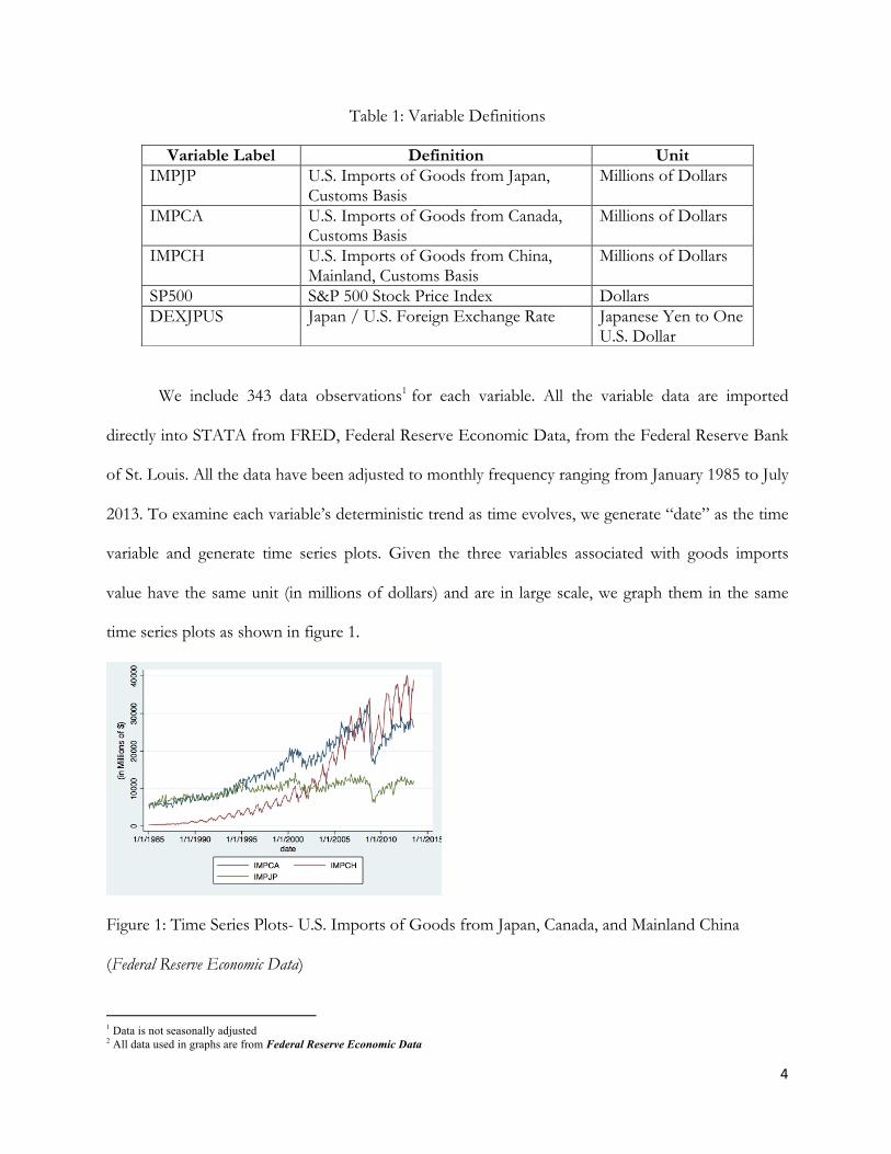
We include 343 data observations1 for each variable. All the variable data are imported

directly into STATA from FRED, Federal Reserve Economic Data, from the Federal Reserve Bank

of St. Louis. All the data have been adjusted to monthly frequency ranging from January 1985 to July

2013. To examine each variable’s deterministic trend as time evolves, we generate “date” as the time

variable and generate time series plots. Given the three variables associated with goods imports

value have the same unit (in millions of dollars) and are in large scale, we graph them in the same

time series plots as shown in figure 1.

Figure 1: Time Series Plots- U.S. Imports of Goods from Japan, Canada, and Mainland China

(Federal Reserve Economic Data)

1 Data is not seasonally adjusted 2 All data used in graphs are from Federal Reserve Economic Data

Variable Label Definition Unit IMPJP U.S. Imports of Goods from Japan,

Customs Basis Millions of Dollars

IMPCA U.S. Imports of Goods from Canada, Customs Basis

Millions of Dollars

IMPCH U.S. Imports of Goods from China, Mainland, Customs Basis

Millions of Dollars

SP500 S&P 500 Stock Price Index Dollars DEXJPUS Japan / U.S. Foreign Exchange Rate Japanese Yen to One

U.S. Dollar

5

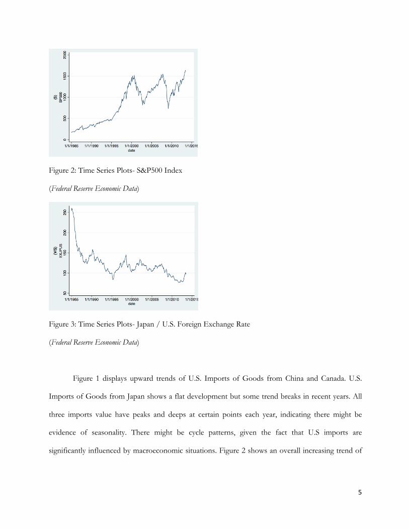
Figure 2: Time Series Plots- S&P500 Index


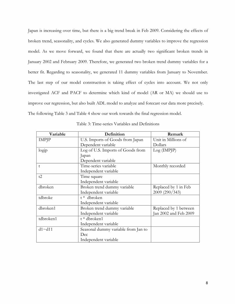
Figure 3: Time Series Plots- Japan / U.S. Foreign Exchange Rate


Figure 1 displays upward trends of U.S. Imports of Goods from China and Canada. U.S.

Imports of Goods from Japan shows a flat development but some trend breaks in recent years. All

three imports value have peaks and deeps at certain points each year, indicating there might be

evidence of seasonality. There might be cycle patterns, given the fact that U.S imports are

significantly influenced by macroeconomic situations. Figure 2 shows an overall increasing trend of

6

S&P 500 Index and two drastic value drops in year 2002 and 2009. Figure 3 shows that the exchange

rate decreases with cycle patterns over time.

To visualize U.S. Imports of Goods from Japan’s relationships with U.S. Imports of Goods

from Canada, U.S. Imports of Goods from Mainland China, S&P 500 Stock Price Index and Japan /

U.S. Foreign Exchange Rate, we generated scatterplots to study the pattern and trend. Based on the

graph shapes, we can use logistic regression for future analysis when including explanatory variables.

Figure 42: IMPJP’s relationship with IMPCA Figure 52: IMPJP’s relationship with IMPCH

Figure 62: IMPJP’s relationship with EXJPUS Figure 73: IMPJP’s relationship with SP500

2 All data used in graphs are from Federal Reserve Economic Data

7

IV. Methodology and Empirical Results

i) Simple Regression Model

Table 2: Variable Definitions

In order to study factors that have main impacts on U.S. Imports of Goods from Japan, we use

IMPJP (U.S. Imports of Goods from Japan) as the dependent variable, and IMPCA (U.S. Imports of

Goods from Canada), IMPCH (U.S. Imports of Goods from China), SP500 (S&P 500 Stock Price

Index), DEXJPUS (Japan / U.S. Foreign Exchange Rate) as independent variables.

• Linear regression equation:

(1)

• Logistic regression equation:

(2)

For future improvements, we can make variations on the logistic regression model by

changing different combinations of variables in log format or use the quadratic regression model to

find the best fit regression equation.

ii) Time-series Regression Model

In order to find the best-fit time-series regression model of U.S. Imports of Goods from

Japan, we generated a new time variable “t” to analyze monthly change of the imports value relative

to time. Because values of U.S. Imports of Goods from Japan are in large scale, we adjusted this

dependent variable to log form in the regression model. The trend of U.S. Imports of Goods from

Variable Label Definition Unit IMPJP U.S. Imports of Goods from Japan,

Customs Basis Millions of Dollars

IMPCA U.S. Imports of Goods from Canada, Customs Basis

Millions of Dollars

IMPCH U.S. Imports of Goods from China, Mainland, Customs Basis

Millions of Dollars

SP500 S&P 500 Stock Price Index Dollars DEXJPUS Japan / U.S. Foreign Exchange Rate Japanese Yen to One

U.S. Dollar

8

Japan is increasing over time, but there is a big trend break in Feb 2009. Considering the effects of

broken trend, seasonality, and cycles. We also generated dummy variables to improve the regression

model. As we move forward, we found that there are actually two significant broken trends in

January 2002 and February 2009. Therefore, we generated two broken trend dummy variables for a

better fit. Regarding to seasonality, we generated 11 dummy variables from January to November.

The last step of our model construction is taking effect of cycles into account. We not only

investigated ACF and PACF to determine which kind of model (AR or MA) we should use to

improve our regression, but also built ADL model to analyze and forecast our data more precisely.

The following Table 3 and Table 4 show our work towards the final regression model.

Table 3: Time-series Variables and Definitions

Variable Definition Remark IMPJP U.S. Imports of Goods from Japan

Dependent variable Unit in Millions of Dollars

logjp Log of U.S. Imports of Goods from Japan Dependent variable

Log (IMPJP)

t Time-series variable Independent variable

Monthly recorded

t2 Time square Independent variable

dbroken Broken trend dummy variable Independent variable

Replaced by 1 in Feb 2009 (290/343)

tdbroke t * dbroken Independent variable

dbroken1 Broken trend dummy variable Independent variable

Replaced by 1 between Jan 2002 and Feb 2009

tdbroken1 t * dbroken1 Independent variable

d1~d11 Seasonal dummy variable from Jan to Dec Independent variable

9

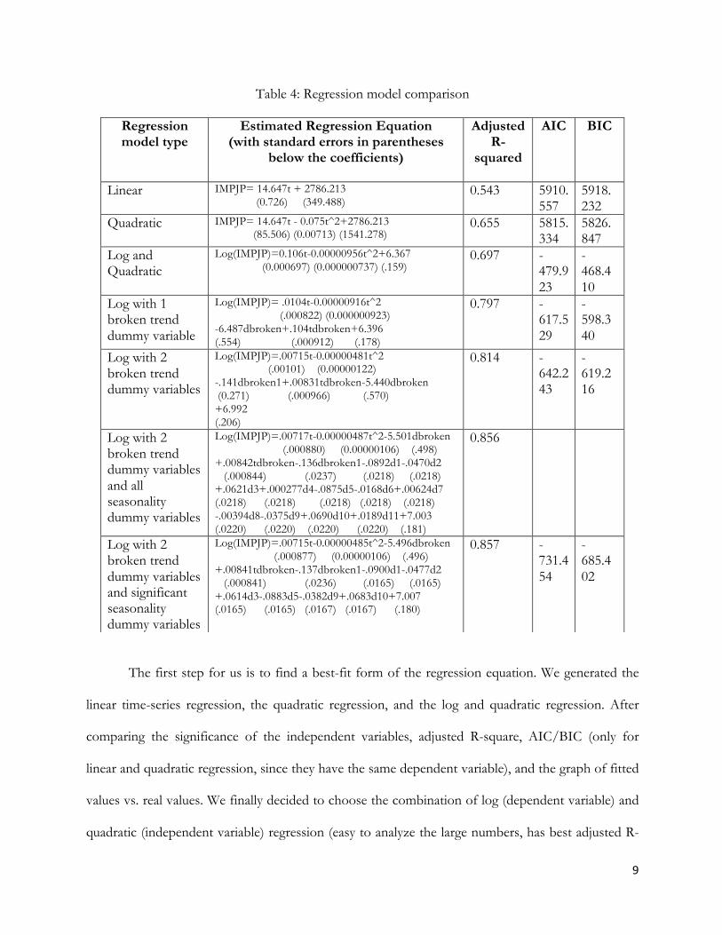
Table 4: Regression model comparison

The first step for us is to find a best-fit form of the regression equation. We generated the

linear time-series regression, the quadratic regression, and the log and quadratic regression. After

comparing the significance of the independent variables, adjusted R-square, AIC/BIC (only for

linear and quadratic regression, since they have the same dependent variable), and the graph of fitted

values vs. real values. We finally decided to choose the combination of log (dependent variable) and

quadratic (independent variable) regression (easy to analyze the large numbers, has best adjusted R-

Regression model type

Estimated Regression Equation (with standard errors in parentheses

below the coefficients)

Adjusted R-

squared

AIC

BIC

Linear IMPJP= 14.647t + 2786.213 (0.726) (349.488)

0.543 5910.557

5918.232

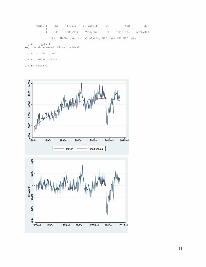
Quadratic IMPJP= 14.647t - 0.075t^2+2786.213 (85.506) (0.00713) (1541.278)

0.655 5815.334

5826.847

Log and Quadratic

Log(IMPJP)=0.106t-0.00000956t^2+6.367 (0.000697) (0.000000737) (.159)

0.697 -479.923

-468.410

Log with 1 broken trend dummy variable

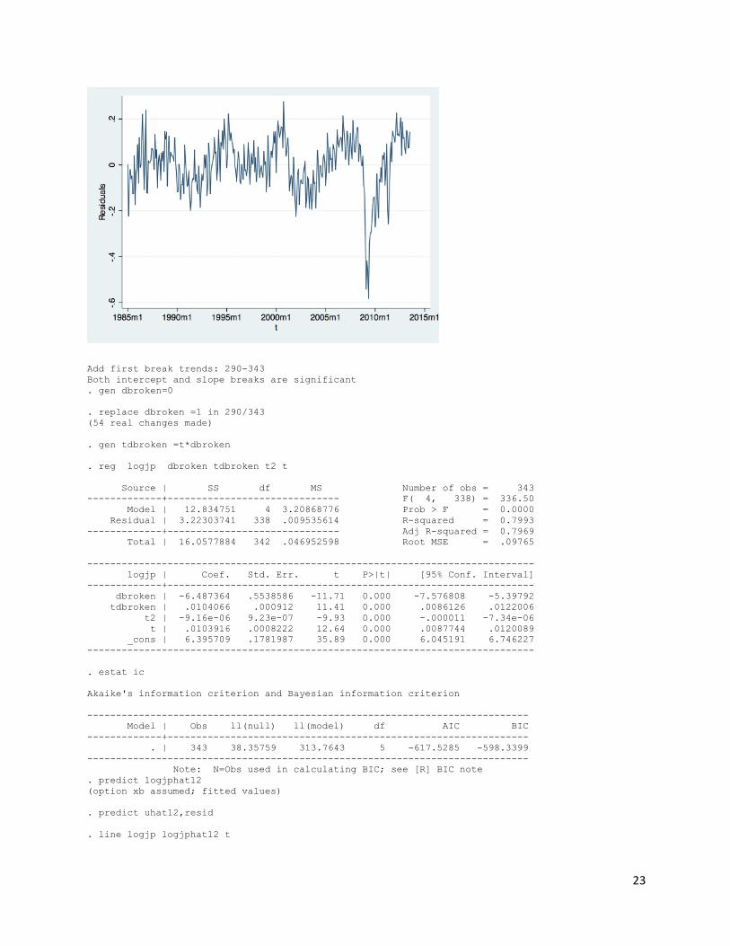
Log(IMPJP)= .0104t-0.00000916t^2 (.000822) (0.000000923) -6.487dbroken+.104tdbroken+6.396 (.554) (.000912) (.178)

0.797 -617.529

-598.340

Log with 2 broken trend dummy variables

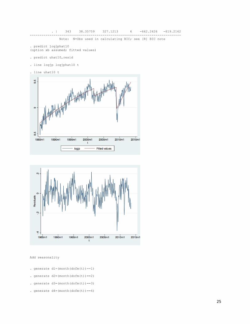
Log(IMPJP)=.00715t-0.00000481t^2 (.00101) (0.00000122) -.141dbroken1+.00831tdbroken-5.440dbroken (0.271) (.000966) (.570) +6.992 (.206)

0.814 -642.243

-619.216

Log with 2 broken trend dummy variables and all seasonality dummy variables

Log(IMPJP)=.00717t-0.00000487t^2-5.501dbroken (.000880) (0.00000106) (.498) +.00842tdbroken-.136dbroken1-.0892d1-.0470d2 (.000844) (.0237) (.0218) (.0218) +.0621d3+.000277d4-.0875d5-.0168d6+.00624d7 (.0218) (.0218) (.0218) (.0218) (.0218) -.00394d8-.0375d9+.0690d10+.0189d11+7.003 (.0220) (.0220) (.0220) (.0220) (.181)

0.856

Log with 2 broken trend dummy variables and significant seasonality dummy variables

Log(IMPJP)=.00715t-0.00000485t^2-5.496dbroken (.000877) (0.00000106) (.496) +.00841tdbroken-.137dbroken1-.0900d1-.0477d2 (.000841) (.0236) (.0165) (.0165) +.0614d3-.0883d5-.0382d9+.0683d10+7.007 (.0165) (.0165) (.0167) (.0167) (.180)

0.857 -731.454

-685.402

10

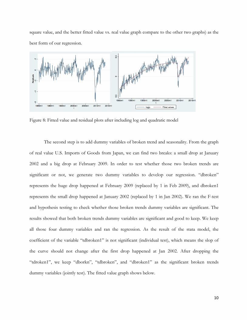
square value, and the better fitted value vs. real value graph compare to the other two graphs) as the

best form of our regression.

Figure 8: Fitted value and residual plots after including log and quadratic model

The second step is to add dummy variables of broken trend and seasonality. From the graph

of real value U.S. Imports of Goods from Japan, we can find two breaks: a small drop at January

2002 and a big drop at February 2009. In order to test whether those two broken trends are

significant or not, we generate two dummy variables to develop our regression. “dbroken”

represents the huge drop happened at February 2009 (replaced by 1 in Feb 2009), and dbroken1

represents the small drop happened at January 2002 (replaced by 1 in Jan 2002). We ran the F-test

and hypothesis testing to check whether those broken trends dummy variables are significant. The

results showed that both broken trends dummy variables are significant and good to keep. We keep

all those four dummy variables and ran the regression. As the result of the stata model, the

coefficient of the variable “tdbroken1” is not significant (individual test), which means the slop of

the curve should not change after the first drop happened at Jan 2002. After dropping the

“tdroken1”, we keep “dborkn”, “tdbroken”, and “dbroken1” as the significant broken trends

dummy variables (jointly test). The fitted value graph shows below.

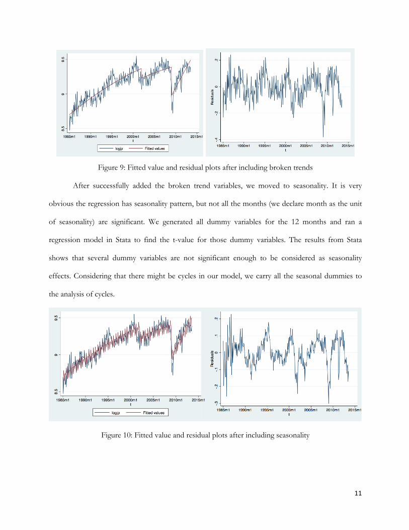
11

Figure 9: Fitted value and residual plots after including broken trends

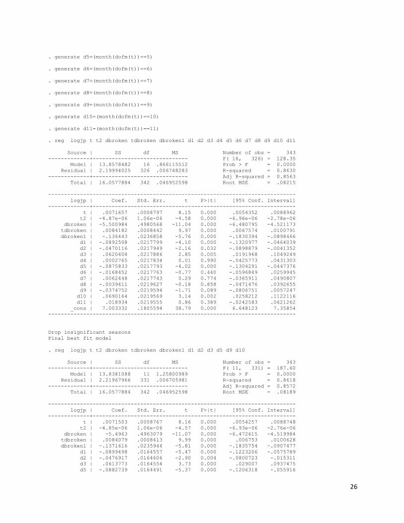
After successfully added the broken trend variables, we moved to seasonality. It is very

obvious the regression has seasonality pattern, but not all the months (we declare month as the unit

of seasonality) are significant. We generated all dummy variables for the 12 months and ran a

regression model in Stata to find the t-value for those dummy variables. The results from Stata

shows that several dummy variables are not significant enough to be considered as seasonality

effects. Considering that there might be cycles in our model, we carry all the seasonal dummies to

the analysis of cycles.

Figure 10: Fitted value and residual plots after including seasonality

12

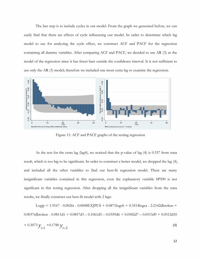
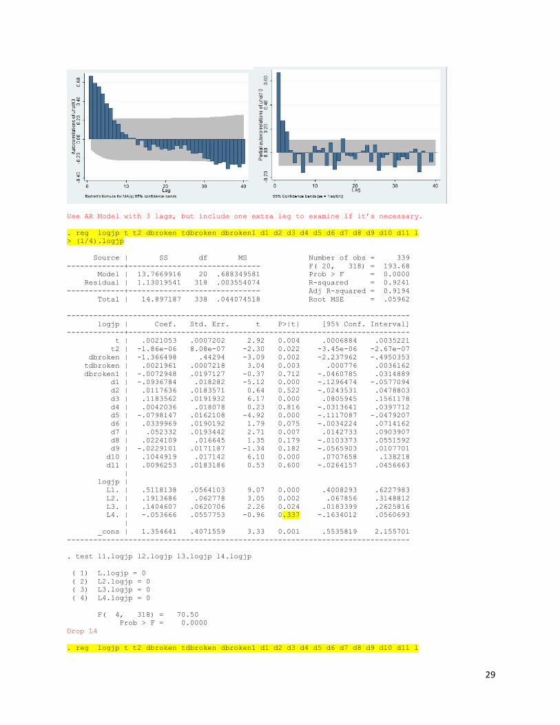
The last step is to include cycles in our model. From the graph we generated before, we can

easily find that there are effects of cycle influencing our model. In order to determine which lag

model to use for analyzing the cycle effect, we construct ACF and PACF for the regression

containing all dummy variables. After comparing ACF and PACF, we decided to use AR (3) as the

model of the regression since it has fewer bars outside the confidence interval. It is not sufficient to

use only the AR (3) model; therefore we included one more extra lag to examine the regression.

Figure 11: ACF and PACF graphs of the testing regression

As the test for the extra lag (lag4), we noticed that the p-value of lag (4) is 0.337 from stata

result, which is too big to be significant. In order to construct a better model, we dropped the lag (4),

and included all the other variables to find our best-fit regression model. There are many

insignificant variables contained in this regression, even the explanatory variable SP500 is not

significant in this testing regression. After dropping all the insignificant variables from the stata

results, we finally construct our best-fit model with 2 lags:

Logjp = 1.9167 - 0.0026t - 0.0008EXJPUS + 0.0871logch + 0.3514logca - 2.2142dbroken +

0.0037tdbroken - 0.0811d1 + 0.0857d3 – 0.1061d5 – 0.0359d6 + 0.0582d7 – 0.0515d9 + 0.0512d10

+ 0.3073 yt−1 +0.1780 yt−2 (3)

13

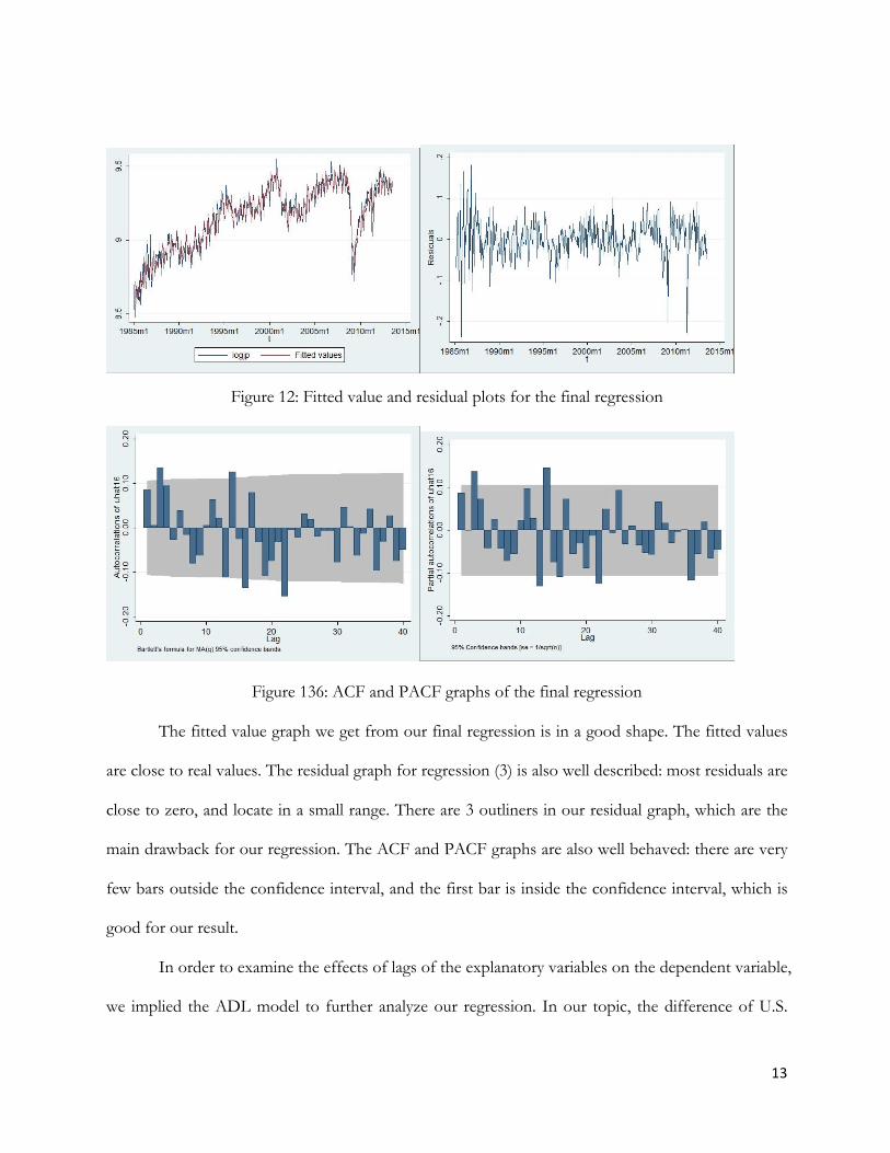
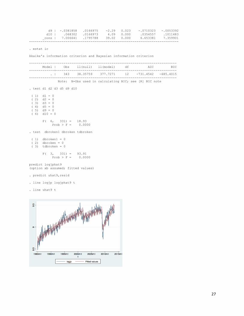
Figure 12: Fitted value and residual plots for the final regression

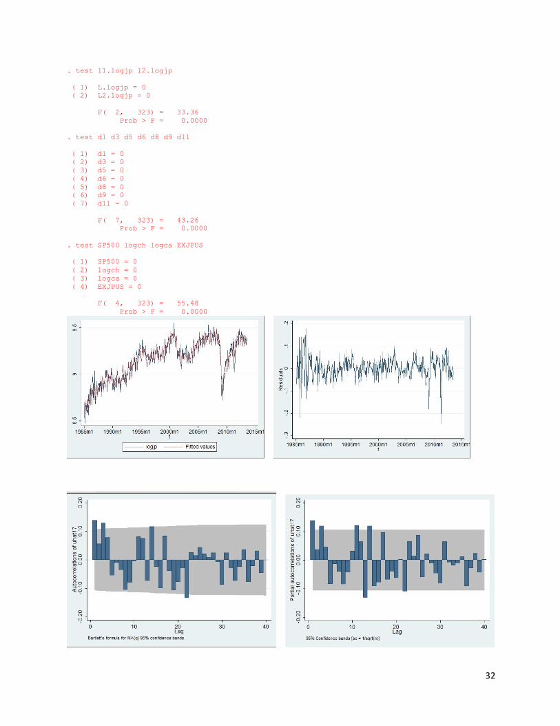
Figure 136: ACF and PACF graphs of the final regression

The fitted value graph we get from our final regression is in a good shape. The fitted values

are close to real values. The residual graph for regression (3) is also well described: most residuals are

close to zero, and locate in a small range. There are 3 outliners in our residual graph, which are the

main drawback for our regression. The ACF and PACF graphs are also well behaved: there are very

few bars outside the confidence interval, and the first bar is inside the confidence interval, which is

good for our result.

In order to examine the effects of lags of the explanatory variables on the dependent variable,

we implied the ADL model to further analyze our regression. In our topic, the difference of U.S.

14

imports of goods from Japan may be affected by the lags of our explanatory variables. We construct

the ADL model between the difference of log U.S. imports of goods from Japan and the Exchange

rate between U.S. dollar and Japanese Yen to find whether there is a relationship between them. As

the result of our ADL model, we can find that the lags of the Exchange rate are significant;

therefore we can state that the lags of Exchange rate affect U.S. imports of goods from Japan.

One-step forecast:

T=343, July, 2013

t = T+1=344, August 2013

Logjpt+1 = 1.9167 - 0.0026(344) - 0.0008(97.86) + 0.0871log(39171.7)+ 0.3514log (27835.3)

- 2.2142(1) + 0.0037(344)(1) + 0.3073(log(11971.3))+0.1780(log(11183.9))= 9.06

Actual U.S. Imports of Goods from Japan:

Log(12067.8)=9.40

We underestimated the U.S. Imports of Goods from Japan.

Two-step forecast:

t = T+2=345, September 2013

Logjpt+2 = 1.9167 - 0.0026(345) - 0.0008(99.23) + 0.0871log(40067.4)+ 0.3514log (28152.5)

- 2.2142(1) + 0.0037(345)(1) – 0.0515(1) + 0.3073(9.06)+0.1780(log(11971.3))= 8.93

Actual U.S. Imports of Goods from Japan:

Log(11052.9)=9.31

We underestimated the U.S. Imports of Goods from Japan.

We generated the best-fit regression including the log form of the dependent variable,

quadratic form of the time-series variable, broken trend dummy variables, seasonality dummy

variables, and cycle effects. From the regression model, we can conclude that the percentage change

of U.S. Imports of Goods from Japan is in an increasing trend with one drop happened at 2009

15

because of the Economic Crisis and other reasons. The seasonality effects on U.S. Imports of

Goods from Japan are more likely to be detected for January, March, May, June, July, September,

and October. There are two lags in our regression, which imply the cycle effects to the model. In

general, the regression predicts the future values of U.S imports of goods from Japan very close to

the real value.

V. Conclusion

In this paper, we mainly focused on finding the factors that affect the U.S. imports of goods

from Japan and constructing time-series regression model to forecast the future value of U.S.

imports of goods from Japan.

We developed our research paper step by step: discuss an real-world issue that worth

analyzing, study the literatures related to the topic, find data from online source, construct the

simple regression model, improve our model with time-series components, conclude the results and

forecast the future values.

In our final regression model, we find that the U.S. imports of goods from Japan is affected

by log of the U.S. imports of goods from China, log of the U.S. imports of goods from Canada, and

the Exchange rate between U.S. dollars and Japanese Yen with the influences of broken trend

variable, seasonality dummy variables, cycles and lags. The fitted values of our regression fit the real

values closely, and the residuals are also located very well. In general, we can use our model to

predict the future values of the U.S. imports of goods from Japan closely, with a small forecast error.

There are some limitations of our paper, such as we cannot eliminate the effects of outliners,

our regression model removes the variable SP500, which should be included as an independent

variable, or the small number of lags may affect our model in forecasting the remote value of U.S.

imports of goods from Japan etc. Although there are many limitations of our paper, the regression

16

we found could still make accurate forecast of the future value and provide sufficient information

for policy makers to make right decision.

17

References

Cooper William H. 2013. “U.S.- Japan Economic Relations: Significance, Prospects, and Policy Options.” Congressional Research Service, August 13. http://www.fas.org/sgp/crs/row/RL32649.pdf

Espinoza Charlotte and Miller Ambassador Terry, Scissors Derek . 2012. “Trade Freedom: How Imports Support U.S. Jobs.” The Heritage Foundation, September 12. http://www.heritage.org/research/reports/2012/09/trade-freedom-how-imports-support-us-jobs

FRED, Federal Reserve Economic Data. 1985-2013. “Japan / U.S. Foreign Exchange Rate (DEXJPUS)”, the Federal Reserve Bank of St. Louis.

http://research.stlouisfed.org/fred2/series/DEXJPUS (accessed October 17, 2013)

“S&P 500 Stock Price Index (SP500)”, the Federal Reserve Bank of St. Louis. http://research.stlouisfed.org/fred2/series/SP500 (accessed October 17, 2013)

“U.S. Imports of Goods from Japan, Customs Basis (IMPJP)”, the Federal Reserve Bank of St. Louis. http://research.stlouisfed.org/fred2/series/IMPJP (accessed October 17, 2013)

“U.S. Imports of Goods from China, Mainland, Customs Basis (IMPCH)”, the Federal Reserve Bank of St. Louis. http://research.stlouisfed.org/fred2/series/IMPCH (accessed October 17, 2013)

“U.S. Imports of Goods from Canada, Customs Basis (IMPCA)”, the Federal Reserve Bank of St. Louis. http://research.stlouisfed.org/fred2/series/IMPCA (accessed October 17, 2013)

Jabara Cathy L. 2009. “How Do Exchange Rate Affect Import Prices? Recent Economic Literature and Data Analysis.” U.S. International Trade Commission, October. http://www.usitc.gov/publications/332/working_papers/id-21_revised.pdf

Trading Economics. "United States Balance Of Trade",. http://www.tradingeconomics.com/united-states/balance-of-trade (accessed October 17, 2013) "United States Imports" http://www.tradingeconomics.com/united-states/imports (accessed October 17, 2013) “U.S. Imports and Exports Components”, About.com. http://useconomy.about.com/od/tradepolicy/p/Imports-Exports-Components.htm(accessed October 17, 2013

18

Appendix A i) Null hypothesis testing for “dborken”, “tdbroken”, “dbroken1”, and “tdbroken1”

H0 : β3 = β4 = β5 = β6 = 0

HA : At least one of them is not zero

Unrestricted regression equation: 6

logjp = α + β1t + β2t2 + β3dbroken + β4tdbroken + β5dbroken1 + β6 tdbroken1+ u

Restricted regression equation:

logjp = α + β1t + β2t2 + u

F-value: 93.91; T-K: 337; Degrees of freedom: 4; Critical Values: between 2.61 and 2.68

Since the F-value is greater than the critical value, we reject the null hypothesis. There is evidence to support the broken trends in the regression model.

ii) Null hypothesis testing for all seasonality dummy variables

H0 : β6 = β7 = β8 = β9 = β10 = β11 = β12 = β13 = β14 = β15 = β16


Unrestricted regression equation:

logjp = α + β1t + β2t2 + β3dbroken + β4tdbroken + β5dbroken1 + β6d1 + β7d2 + β8d3 + β9d4 + β10d5 + β11d6 + β12d7 + β13d8 + β14d9 + β15d10 + β16d11 + u

Restricted regression equation:

logjp = α + β1t + β2t2 + β3dbroken + β4tdbroken + β5dbroken1 + u

F-value: 18.93; T-K: 331; Degrees of freedom: 10; Critical Values: between 2.22 and 2.29

Since the F-value is greater than the critical value, we reject the null hypothesis. There is evidence to support the seasonality in the regression model

iii) Null hypothesis testing for “l1.logjp”, “l2.logjp”, “l3.logjp”, and “l4.logjp”

H0 : γ1 = γ2 = γ3 = γ4


From stata result, we can find that the F-value of the test is 70.50, which is much larger than the critical value. We can also get the same result from checking p-value: 0.0000.

In general, we can reject the null hypothesis and state that the coefficients of lags are not zero, which means those lags are significant.

19

iv) Null hypothesis testing for “l1.EXJPUS” and “l2.EXJPUS)

H0 : γ1 = γ2


From stata result, we can find that the F-value of the test is 6.15, which is greater than the critical value. We also catch the same result from the p-value: 0.0024, which is smaller than 0.005.

In general, we can reject the null hypothesis, and state that the coefficients of lags are not zero, which means those lags are significant.

Appendix B . gen t=m(1985m1)+_n-1 . format t %tm . tsset t time variable: t, 1985m1 to 2013m7 delta: 1 month . line IMPJP t . reg IMPJP t Source | SS df MS Number of obs = 343 -------------+------------------------------ F( 1, 341) = 406.84 Model | 721384034 1 721384034 Prob > F = 0.0000 Residual | 604635396 341 1773124.33 R-squared = 0.5440 -------------+------------------------------ Adj R-squared = 0.5427 Total | 1.3260e+09 342 3877249.79 Root MSE = 1331.6 ------------------------------------------------------------------------------ IMPJP | Coef. Std. Err. t P>|t| [95% Conf. Interval] -------------+---------------------------------------------------------------- t | 14.64652 .7261409 20.17 0.000 13.21824 16.0748 _cons | 2786.213 349.4881 7.97 0.000 2098.789 3473.636 ------------------------------------------------------------------------------ . predict jphat (option xb assumed; fitted values) . predict uhat, resid . estat ic Akaike's information criterion and Bayesian information criterion ----------------------------------------------------------------------------- Model | Obs ll(null) ll(model) df AIC BIC -------------+--------------------------------------------------------------- . | 343 -3087.959 -2953.279 2 5910.557 5918.232 ----------------------------------------------------------------------------- Note: N=Obs used in calculating BIC; see [R] BIC note . line IMPJP jphat t

20

. line uhat t

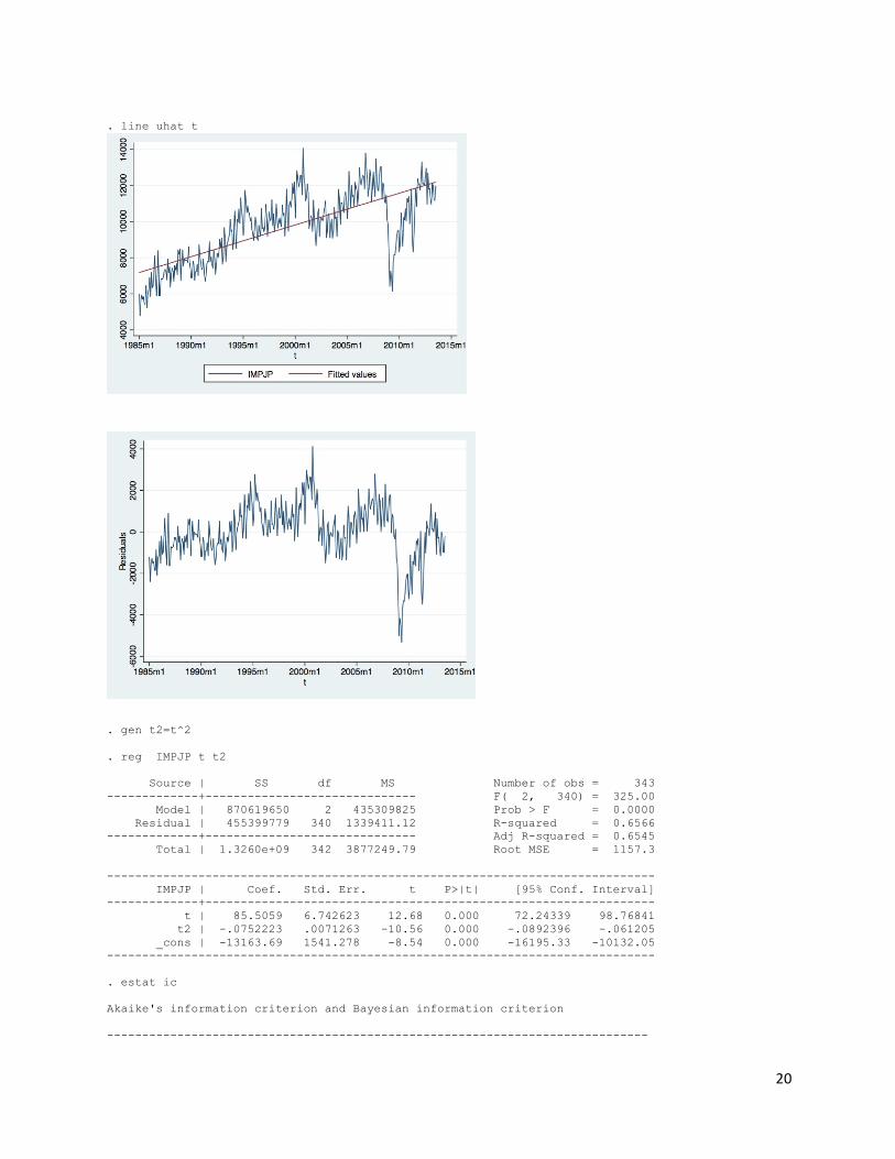
. gen t2=t^2 . reg IMPJP t t2 Source | SS df MS Number of obs = 343 -------------+------------------------------ F( 2, 340) = 325.00 Model | 870619650 2 435309825 Prob > F = 0.0000 Residual | 455399779 340 1339411.12 R-squared = 0.6566 -------------+------------------------------ Adj R-squared = 0.6545 Total | 1.3260e+09 342 3877249.79 Root MSE = 1157.3 ------------------------------------------------------------------------------ IMPJP | Coef. Std. Err. t P>|t| [95% Conf. Interval] -------------+---------------------------------------------------------------- t | 85.5059 6.742623 12.68 0.000 72.24339 98.76841 t2 | -.0752223 .0071263 -10.56 0.000 -.0892396 -.061205 _cons | -13163.69 1541.278 -8.54 0.000 -16195.33 -10132.05 ------------------------------------------------------------------------------ . estat ic Akaike's information criterion and Bayesian information criterion -----------------------------------------------------------------------------

21

Model | Obs ll(null) ll(model) df AIC BIC -------------+--------------------------------------------------------------- . | 343 -3087.959 -2904.667 3 5815.334 5826.847 ----------------------------------------------------------------------------- Note: N=Obs used in calculating BIC; see [R] BIC note . predict jphat2 (option xb assumed; fitted values) . predict uhat2,resid . line IMPJP jphat2 t . line uhat2 t

22

. rename logjapan logjp . reg logjp t t2 Source | SS df MS Number of obs = 343 -------------+------------------------------ F( 2, 340) = 390.50 Model | 11.1874314 2 5.5937157 Prob > F = 0.0000 Residual | 4.87035704 340 .01432458 R-squared = 0.6967 -------------+------------------------------ Adj R-squared = 0.6949 Total | 16.0577884 342 .046952598 Root MSE = .11969 ------------------------------------------------------------------------------ logjp | Coef. Std. Err. t P>|t| [95% Conf. Interval] -------------+---------------------------------------------------------------- t | .010625 .0006973 15.24 0.000 .0092534 .0119965 t2 | -9.56e-06 7.37e-07 -12.98 0.000 -.000011 -8.11e-06 _cons | 6.367127 .1593914 39.95 0.000 6.053609 6.680644 ------------------------------------------------------------------------------ . estat ic Akaike's information criterion and Bayesian information criterion ----------------------------------------------------------------------------- Model | Obs ll(null) ll(model) df AIC BIC -------------+--------------------------------------------------------------- . | 343 38.35759 242.9617 3 -479.9233 -468.4102 ----------------------------------------------------------------------------- Note: N=Obs used in calculating BIC; see [R] BIC note . predict logjphat (option xb assumed; fitted values) . predict uhat3, resid . rename logjphat logjphat3 . line logjp logjphat3 t . line uhat3 t . line logjp logjphat3 t

23

Add first break trends: 290-343 Both intercept and slope breaks are significant . gen dbroken=0 . replace dbroken =1 in 290/343 (54 real changes made) . gen tdbroken =t*dbroken . reg logjp dbroken tdbroken t2 t Source | SS df MS Number of obs = 343 -------------+------------------------------ F( 4, 338) = 336.50 Model | 12.834751 4 3.20868776 Prob > F = 0.0000 Residual | 3.22303741 338 .009535614 R-squared = 0.7993 -------------+------------------------------ Adj R-squared = 0.7969 Total | 16.0577884 342 .046952598 Root MSE = .09765 ------------------------------------------------------------------------------ logjp | Coef. Std. Err. t P>|t| [95% Conf. Interval] -------------+---------------------------------------------------------------- dbroken | -6.487364 .5538586 -11.71 0.000 -7.576808 -5.39792 tdbroken | .0104066 .000912 11.41 0.000 .0086126 .0122006 t2 | -9.16e-06 9.23e-07 -9.93 0.000 -.000011 -7.34e-06 t | .0103916 .0008222 12.64 0.000 .0087744 .0120089 _cons | 6.395709 .1781987 35.89 0.000 6.045191 6.746227 ------------------------------------------------------------------------------ . estat ic Akaike's information criterion and Bayesian information criterion ----------------------------------------------------------------------------- Model | Obs ll(null) ll(model) df AIC BIC -------------+--------------------------------------------------------------- . | 343 38.35759 313.7643 5 -617.5285 -598.3399 ----------------------------------------------------------------------------- Note: N=Obs used in calculating BIC; see [R] BIC note . predict logjphat12 (option xb assumed; fitted values) . predict uhat12,resid . line logjp logjphat12 t

24

. line uhat12 t

Add another break trends 205-289, only intercept break, no slope break(drop it) .reg logjp dbroken tdbroken dbroken1 t2 t Source | SS df MS Number of obs = 343 -------------+------------------------------ F( 5, 337) = 295.60 Model | 13.0762469 5 2.61524937 Prob > F = 0.0000 Residual | 2.98154157 337 .008847304 R-squared = 0.8143 -------------+------------------------------ Adj R-squared = 0.8116 Total | 16.0577884 342 .046952598 Root MSE = .09406 ------------------------------------------------------------------------------ logjp | Coef. Std. Err. t P>|t| [95% Conf. Interval] -------------+---------------------------------------------------------------- dbroken | -5.440048 .5699131 -9.55 0.000 -6.561083 -4.319013 tdbroken | .0083075 .000966 8.60 0.000 .0064072 .0102077 dbroken1 | -.1414444 .027073 -5.22 0.000 -.1946977 -.088191 t2 | -4.81e-06 1.22e-06 -3.96 0.000 -7.21e-06 -2.42e-06 t | .0071452 .0010066 7.10 0.000 .0051651 .0091252 _cons | 6.992457 .2061766 33.91 0.000 6.586902 7.398012 ------------------------------------------------------------------------------ . estat ic Akaike's information criterion and Bayesian information criterion ----------------------------------------------------------------------------- Model | Obs ll(null) ll(model) df AIC BIC -------------+---------------------------------------------------------------

25

. | 343 38.35759 327.1213 6 -642.2426 -619.2162 ----------------------------------------------------------------------------- Note: N=Obs used in calculating BIC; see [R] BIC note . predict logjphat10 (option xb assumed; fitted values) . predict uhat10,resid . line logjp logjphat10 t . line uhat10 t

Add seasonality . generate d1=(month(dofm(t))==1) . generate d2=(month(dofm(t))==2) . generate d3=(month(dofm(t))==3) . generate d4=(month(dofm(t))==4)

26

. generate d5=(month(dofm(t))==5) . generate d6=(month(dofm(t))==6) . generate d7=(month(dofm(t))==7) . generate d8=(month(dofm(t))==8) . generate d9=(month(dofm(t))==9) . generate d10=(month(dofm(t))==10) . generate d11=(month(dofm(t))==11) . reg logjp t t2 dbroken tdbroken dbroken1 d1 d2 d3 d4 d5 d6 d7 d8 d9 d10 d11 Source | SS df MS Number of obs = 343 -------------+------------------------------ F( 16, 326) = 128.35 Model | 13.8578482 16 .866115512 Prob > F = 0.0000 Residual | 2.19994025 326 .006748283 R-squared = 0.8630 -------------+------------------------------ Adj R-squared = 0.8563 Total | 16.0577884 342 .046952598 Root MSE = .08215 ------------------------------------------------------------------------------ logjp | Coef. Std. Err. t P>|t| [95% Conf. Interval] -------------+---------------------------------------------------------------- t | .0071657 .0008797 8.15 0.000 .0054352 .0088962 t2 | -4.87e-06 1.06e-06 -4.58 0.000 -6.96e-06 -2.78e-06 dbroken | -5.500984 .4980568 -11.04 0.000 -6.480795 -4.521173 tdbroken | .0084182 .0008442 9.97 0.000 .0067574 .0100791 dbroken1 | -.136443 .0236858 -5.76 0.000 -.1830394 -.0898466 d1 | -.0892508 .0217799 -4.10 0.000 -.1320977 -.0464039 d2 | -.0470116 .0217949 -2.16 0.032 -.0898879 -.0041352 d3 | .0620608 .0217886 2.85 0.005 .0191968 .1049249 d4 | .0002765 .0217834 0.01 0.990 -.0425773 .0431303 d5 | -.0875833 .0217793 -4.02 0.000 -.1304291 -.0447376 d6 | -.0168452 .0217763 -0.77 0.440 -.0596849 .0259945 d7 | .0062448 .0217743 0.29 0.774 -.0365911 .0490807 d8 | -.0039411 .0219627 -0.18 0.858 -.0471476 .0392655 d9 | -.0374752 .0219594 -1.71 0.089 -.0806751 .0057247 d10 | .0690164 .0219569 3.14 0.002 .0258212 .1122116 d11 | .018934 .0219555 0.86 0.389 -.0242583 .0621262 _cons | 7.003332 .1805594 38.79 0.000 6.648123 7.35854 ------------------------------------------------------------------------------ Drop insignificant seasons Final best fit model . reg logjp t t2 dbroken tdbroken dbroken1 d1 d2 d3 d5 d9 d10 Source | SS df MS Number of obs = 343 -------------+------------------------------ F( 11, 331) = 187.60 Model | 13.8381088 11 1.25800989 Prob > F = 0.0000 Residual | 2.21967966 331 .006705981 R-squared = 0.8618 -------------+------------------------------ Adj R-squared = 0.8572 Total | 16.0577884 342 .046952598 Root MSE = .08189 ------------------------------------------------------------------------------ logjp | Coef. Std. Err. t P>|t| [95% Conf. Interval] -------------+---------------------------------------------------------------- t | .0071503 .0008767 8.16 0.000 .0054257 .0088748 t2 | -4.85e-06 1.06e-06 -4.57 0.000 -6.93e-06 -2.76e-06 dbroken | -5.4963 .4963079 -11.07 0.000 -6.472615 -4.519984 tdbroken | .0084079 .0008413 9.99 0.000 .006753 .0100628 dbroken1 | -.1371616 .0235944 -5.81 0.000 -.1835754 -.0907477 d1 | -.0899498 .0164557 -5.47 0.000 -.1223206 -.0575789 d2 | -.0476917 .0164606 -2.90 0.004 -.0800723 -.015311 d3 | .0613773 .0164554 3.73 0.000 .029007 .0937475 d5 | -.0882739 .0164491 -5.37 0.000 -.1206318 -.055916

27

d9 | -.0381858 .0166975 -2.29 0.023 -.0710323 -.0053392 d10 | .068302 .0166973 4.09 0.000 .0354557 .1011483 _cons | 7.006641 .1795788 39.02 0.000 6.653381 7.359901 ------------------------------------------------------------------------------ . estat ic Akaike's information criterion and Bayesian information criterion ----------------------------------------------------------------------------- Model | Obs ll(null) ll(model) df AIC BIC -------------+--------------------------------------------------------------- . | 343 38.35759 377.7271 12 -731.4542 -685.4015 ----------------------------------------------------------------------------- Note: N=Obs used in calculating BIC; see [R] BIC note . test d1 d2 d3 d5 d9 d10 ( 1) d1 = 0 ( 2) d2 = 0 ( 3) d3 = 0 ( 4) d5 = 0 ( 5) d9 = 0 ( 6) d10 = 0 F( 6, 331) = 18.93 Prob > F = 0.0000 . test dbroken1 dbroken tdbroken ( 1) dbroken1 = 0 ( 2) dbroken = 0 ( 3) tdbroken = 0 F( 3, 331) = 93.91 Prob > F = 0.0000 predict logjphat9 (option xb assumed; fitted values) . predict uhat9,resid . line logjp logjphat9 t . line uhat9 t

28

. reg logjp t t2 dbroken tdbroken dbroken1 d1 d2 d3 d4 d5 d6 d7 d8 d9 d10 d11 Source | SS df MS Number of obs = 343 -------------+------------------------------ F( 16, 326) = 128.35 Model | 13.8578482 16 .866115512 Prob > F = 0.0000 Residual | 2.19994025 326 .006748283 R-squared = 0.8630 -------------+------------------------------ Adj R-squared = 0.8563 Total | 16.0577884 342 .046952598 Root MSE = .08215 ------------------------------------------------------------------------------ logjp | Coef. Std. Err. t P>|t| [95% Conf. Interval] -------------+---------------------------------------------------------------- t | .0071657 .0008797 8.15 0.000 .0054352 .0088962 t2 | -4.87e-06 1.06e-06 -4.58 0.000 -6.96e-06 -2.78e-06 dbroken | -5.500984 .4980568 -11.04 0.000 -6.480795 -4.521173 tdbroken | .0084182 .0008442 9.97 0.000 .0067574 .0100791 dbroken1 | -.136443 .0236858 -5.76 0.000 -.1830394 -.08984666 d1 | -.0892508 .0217799 -4.10 0.000 -.1320977 -.0464039 d2 | -.0470116 .0217949 -2.16 0.032 -.0898879 -.0041352 d3 | .0620608 .0217886 2.85 0.005 .0191968 .1049249 d4 | .0002765 .0217834 0.01 0.990 -.0425773 .0431303 d5 | -.0875833 .0217793 -4.02 0.000 -.1304291 -.0447376 d6 | -.0168452 .0217763 -0.77 0.440 -.0596849 .0259945 d7 | .0062448 .0217743 0.29 0.774 -.0365911 .0490807 d8 | -.0039411 .0219627 -0.18 0.858 -.0471476 .0392655 d9 | -.0374752 .0219594 -1.71 0.089 -.0806751 .0057247 d10 | .0690164 .0219569 3.14 0.002 .0258212 .1122116 d11 | .018934 .0219555 0.86 0.389 -.0242583 .0621262 _cons | 7.003332 .1805594 38.79 0.000 6.648123 7.35854 ------------------------------------------------------------------------------ . estat ic ----------------------------------------------------------------------------- Model | Obs ll(null) ll(model) df AIC BIC -------------+--------------------------------------------------------------- . | 343 38.35759 379.2591 17 -724.5182 -659.2767 ----------------------------------------------------------------------------- Note: N=Obs used in calculating BIC; see [R] BIC note . predict uhat13,resid . ac uhat13,recast(bar) . pac uhat13,recast(bar)

29

Use AR Model with 3 lags, but include one extra leg to examine if it’s necessary. . reg logjp t t2 dbroken tdbroken dbroken1 d1 d2 d3 d4 d5 d6 d7 d8 d9 d10 d11 l > (1/4).logjp Source | SS df MS Number of obs = 339 -------------+------------------------------ F( 20, 318) = 193.68 Model | 13.7669916 20 .688349581 Prob > F = 0.0000 Residual | 1.13019541 318 .003554074 R-squared = 0.9241 -------------+------------------------------ Adj R-squared = 0.9194 Total | 14.897187 338 .044074518 Root MSE = .05962 ------------------------------------------------------------------------------ logjp | Coef. Std. Err. t P>|t| [95% Conf. Interval] -------------+---------------------------------------------------------------- t | .0021053 .0007202 2.92 0.004 .0006884 .0035221 t2 | -1.86e-06 8.08e-07 -2.30 0.022 -3.45e-06 -2.67e-07 dbroken | -1.366498 .44294 -3.09 0.002 -2.237962 -.4950353 tdbroken | .0021961 .0007218 3.04 0.003 .000776 .0036162 dbroken1 | -.0072948 .0197127 -0.37 0.712 -.0460785 .0314889 d1 | -.0936784 .018282 -5.12 0.000 -.1296474 -.0577094 d2 | .0117636 .0183571 0.64 0.522 -.0243531 .0478803 d3 | .1183562 .0191932 6.17 0.000 .0805945 .1561178 d4 | .0042036 .018078 0.23 0.816 -.0313641 .0397712 d5 | -.0798147 .0162108 -4.92 0.000 -.1117087 -.0479207 d6 | .0339969 .0190192 1.79 0.075 -.0034224 .0714162 d7 | .052332 .0193442 2.71 0.007 .0142733 .0903907 d8 | .0224109 .016645 1.35 0.179 -.0103373 .0551592 d9 | -.0229101 .0171187 -1.34 0.182 -.0565903 .0107701 d10 | .1044919 .017142 6.10 0.000 .0707658 .138218 d11 | .0096253 .0183186 0.53 0.600 -.0264157 .0456663 | logjp | L1. | .5118138 .0564103 9.07 0.000 .4008293 .6227983 L2. | .1913686 .062778 3.05 0.002 .067856 .3148812 L3. | .1404607 .0620706 2.26 0.024 .0183399 .2625816 L4. | -.053666 .0557753 -0.96 0.337 -.1634012 .0560693 | _cons | 1.354641 .4071559 3.33 0.001 .5535819 2.155701 ------------------------------------------------------------------------------ . test l1.logjp l2.logjp l3.logjp l4.logjp ( 1) L.logjp = 0 ( 2) L2.logjp = 0 ( 3) L3.logjp = 0 ( 4) L4.logjp = 0 F( 4, 318) = 70.50 Prob > F = 0.0000 Drop L4 . reg logjp t t2 dbroken tdbroken dbroken1 d1 d2 d3 d4 d5 d6 d7 d8 d9 d10 d11 l

30

> (1/3).logjp Source | SS df MS Number of obs = 340 -------------+------------------------------ F( 19, 320) = 207.26 Model | 13.9850139 19 .736053361 Prob > F = 0.0000 Residual | 1.13641516 320 .003551297 R-squared = 0.9248 -------------+------------------------------ Adj R-squared = 0.9204 Total | 15.121429 339 .044605985 Root MSE = .05959 ------------------------------------------------------------------------------ logjp | Coef. Std. Err. t P>|t| [95% Conf. Interval] -------------+---------------------------------------------------------------- t | .0020026 .0007156 2.80 0.005 .0005947 .0034105 t2 | -1.79e-06 8.04e-07 -2.23 0.027 -3.37e-06 -2.10e-07 dbroken | -1.327777 .4404013 -3.01 0.003 -2.194224 -.4613289 tdbroken | .0021429 .0007191 2.98 0.003 .0007281 .0035577 dbroken1 | -.004518 .0192991 -0.23 0.815 -.0424871 .0334511 d1 | -.0913033 .0177789 -5.14 0.000 -.1262816 -.056325 d2 | .0063143 .0177808 0.36 0.723 -.0286678 .0412964 d3 | .1139 .018887 6.03 0.000 .0767416 .1510585 d4 | .0025952 .0177616 0.15 0.884 -.032349 .0375394 d5 | -.0764745 .0158207 -4.83 0.000 -.1076003 -.0453487 d6 | .0357681 .0185485 1.93 0.055 -.0007243 .0722606 d7 | .0462977 .0187381 2.47 0.014 .0094322 .0831631 d8 | .0197509 .0164638 1.20 0.231 -.0126401 .0521419 d9 | -.0193817 .0164725 -1.18 0.240 -.0517897 .0130263 d10 | .1038905 .017067 6.09 0.000 .0703127 .1374683 d11 | .0079258 .018257 0.43 0.664 -.0279931 .0438447 | logjp | L1. | .5034354 .0559822 8.99 0.000 .3932958 .6135751 L2. | .1736841 .0612867 2.83 0.005 .0531082 .2942599 L3. | .1243635 .055659 2.23 0.026 .0148598 .2338673 | _cons | 1.282471 .3867512 3.32 0.001 .5215745 2.043367 ------------------------------------------------------------------------------ Include explanatory variables . reg logjp t t2 EXJPUS logch logca SP500 dbroken tdbroken dbroken1 tdbroken1 d > 1 d2 d3 d4 d5 d6 d7 d8 d9 d10 d11 l(1/3).logjp Source | SS df MS Number of obs = 340 -------------+------------------------------ F( 24, 315) = 235.27 Model | 14.3224323 24 .596768014 Prob > F = 0.0000 Residual | .798996677 315 .002536497 R-squared = 0.9472 -------------+------------------------------ Adj R-squared = 0.9431 Total | 15.121429 339 .044605985 Root MSE = .05036 ------------------------------------------------------------------------------ logjp | Coef. Std. Err. t P>|t| [95% Conf. Interval] -------------+---------------------------------------------------------------- t | -.0091473 .0025943 -3.53 0.000 -.0142517 -.0040429 t2 | 5.53e-06 2.68e-06 2.06 0.040 2.61e-07 .0000108 EXJPUS | -.0012527 .0002459 -5.09 0.000 -.0017365 -.0007689 logch | .193691 .0352036 5.50 0.000 .124427 .262955 logca | .3108651 .0431438 7.21 0.000 .2259787 .3957515 SP500 | .0000841 .0000273 3.08 0.002 .0000304 .0001378 dbroken | -1.413702 .5495358 -2.57 0.011 -2.494927 -.3324779 tdbroken | .0022327 .0010058 2.22 0.027 .0002539 .0042116 dbroken1 | .5757188 .3547294 1.62 0.106 -.1222197 1.273657 tdbroken1 | -.0011139 .0007193 -1.55 0.122 -.0025292 .0003013 d1 | -.1166059 .0153939 -7.57 0.000 -.1468937 -.0863181 d2 | -.0193463 .015346 -1.26 0.208 -.04954 .0108474 d3 | .0693739 .0175198 3.96 0.000 .0349033 .1038445 d4 | -.0215177 .0154548 -1.39 0.165 -.0519254 .00889 d5 | -.1269223 .0142061 -8.93 0.000 -.1548731 -.0989715 d6 | -.0463866 .0173357 -2.68 0.008 -.080495 -.0122782 d7 | .0041707 .0177993 0.23 0.815 -.0308498 .0391913 d8 | -.04956 .0163549 -3.03 0.003 -.0817386 -.0173814 d9 | -.0956554 .0164305 -5.82 0.000 -.1279829 -.063328

31

d10 | .0026789 .0178615 0.15 0.881 -.032464 .0378218 d11 | -.0390219 .0162862 -2.40 0.017 -.0710653 -.0069784 | logjp | L1. | .2729129 .051746 5.27 0.000 .1711015 .3747243 L2. | .1041074 .0528129 1.97 0.050 .0001967 .208018 L3. | .0580249 .0478877 1.21 0.227 -.0361953 .1522451 | _cons | 3.696693 .6671508 5.54 0.000 2.384058 5.009328 . estat ic ----------------------------------------------------------------------------- Model | Obs ll(null) ll(model) df AIC BIC -------------+--------------------------------------------------------------- . | 340 46.74246 546.6294 25 -1043.259 -947.5352 ----------------------------------------------------------------------------- Note: N=Obs used in calculating BIC; see [R] BIC note Drop insignificant variables, drop lag 3 2 final results: need to compare. FIRST ONE . reg logjp t t2 EXJPUS logch logca SP500 dbroken tdbroken d1 d3 d5 d6 d8 d9 d1 > 1 l(1/2).logjp Source | SS df MS Number of obs = 341 -------------+------------------------------ F( 17, 323) = 327.92 Model | 14.5366733 17 .855098427 Prob > F = 0.0000 Residual | .842278808 323 .002607674 R-squared = 0.9452 -------------+------------------------------ Adj R-squared = 0.9423 Total | 15.3789521 340 .045232212 Root MSE = .05107 ------------------------------------------------------------------------------ logjp | Coef. Std. Err. t P>|t| [95% Conf. Interval] -------------+---------------------------------------------------------------- t | -.0070558 .0009582 -7.36 0.000 -.008941 -.0051707 t2 | 3.00e-06 7.73e-07 3.89 0.000 1.48e-06 4.52e-06 EXJPUS | -.0012239 .0002191 -5.59 0.000 -.001655 -.0007929 logch | .2000941 .0213523 9.37 0.000 .158087 .2421012 logca | .3014297 .0376148 8.01 0.000 .2274287 .3754307 SP500 | .0001027 .0000223 4.60 0.000 .0000588 .0001466 dbroken | -2.178065 .3731079 -5.84 0.000 -2.912093 -1.444036 tdbroken | .0036101 .0006081 5.94 0.000 .0024138 .0048063 d1 | -.1052555 .0106632 -9.87 0.000 -.1262336 -.0842774 d3 | .0777398 .0120808 6.43 0.000 .0539727 .1015068 d5 | -.1219292 .0109053 -11.18 0.000 -.1433837 -.1004747 d6 | -.0358541 .0114654 -3.13 0.002 -.0584104 -.0132977 d8 | -.0478425 .0111019 -4.31 0.000 -.0696836 -.0260014 d9 | -.0894685 .0110926 -8.07 0.000 -.1112915 -.0676456 d11 | -.0307971 .0112626 -2.73 0.007 -.0529544 -.0086398 | logjp | L1. | .2644955 .0422752 6.26 0.000 .181326 .3476651 L2. | .1113052 .0396217 2.81 0.005 .033356 .1892544 | _cons | 3.82487 .4345225 8.80 0.000 2.970018 4.679721 ------------------------------------------------------------------------------ . estat ic ----------------------------------------------------------------------------- Model | Obs ll(null) ll(model) df AIC BIC -------------+--------------------------------------------------------------- . | 341 44.50145 539.7433 18 -1043.487 -974.5126 ----------------------------------------------------------------------------- Note: N=Obs used in calculating BIC; see [R] BIC note

32

. test l1.logjp l2.logjp ( 1) L.logjp = 0 ( 2) L2.logjp = 0 F( 2, 323) = 33.36 Prob > F = 0.0000 . test d1 d3 d5 d6 d8 d9 d11 ( 1) d1 = 0 ( 2) d3 = 0 ( 3) d5 = 0 ( 4) d6 = 0 ( 5) d8 = 0 ( 6) d9 = 0 ( 7) d11 = 0 F( 7, 323) = 43.26 Prob > F = 0.0000 . test SP500 logch logca EXJPUS ( 1) SP500 = 0 ( 2) logch = 0 ( 3) logca = 0 ( 4) EXJPUS = 0 F( 4, 323) = 55.48 Prob > F = 0.0000

33

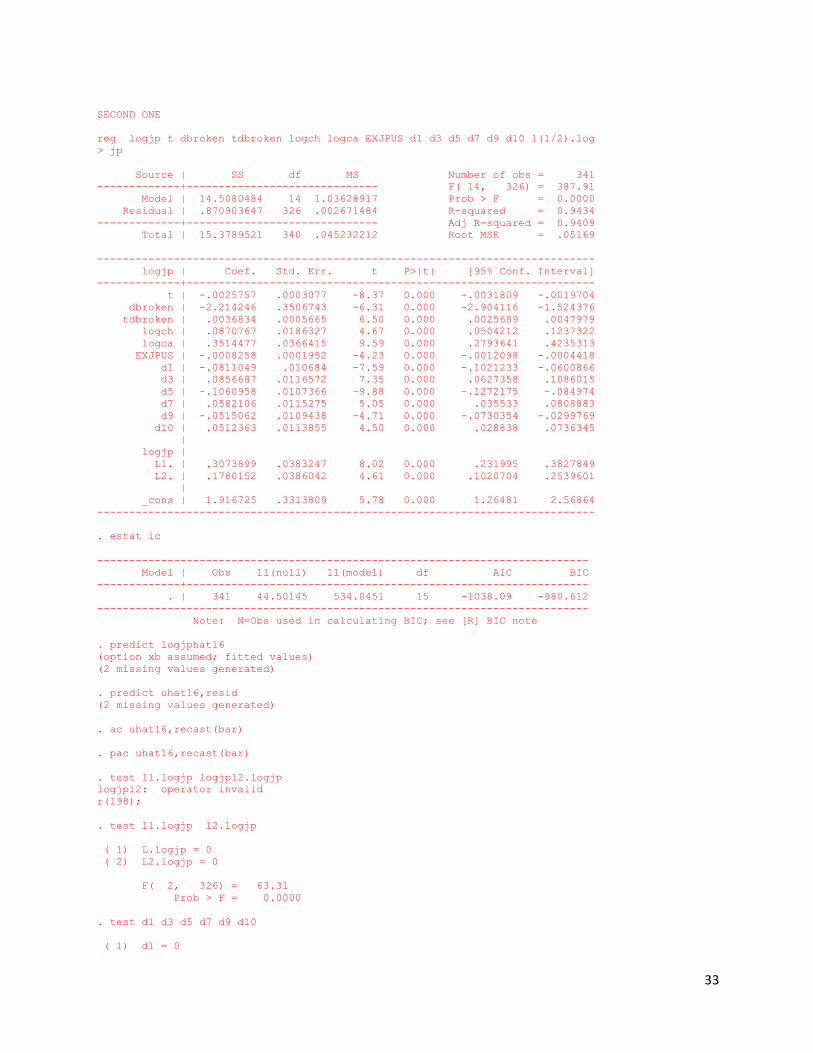
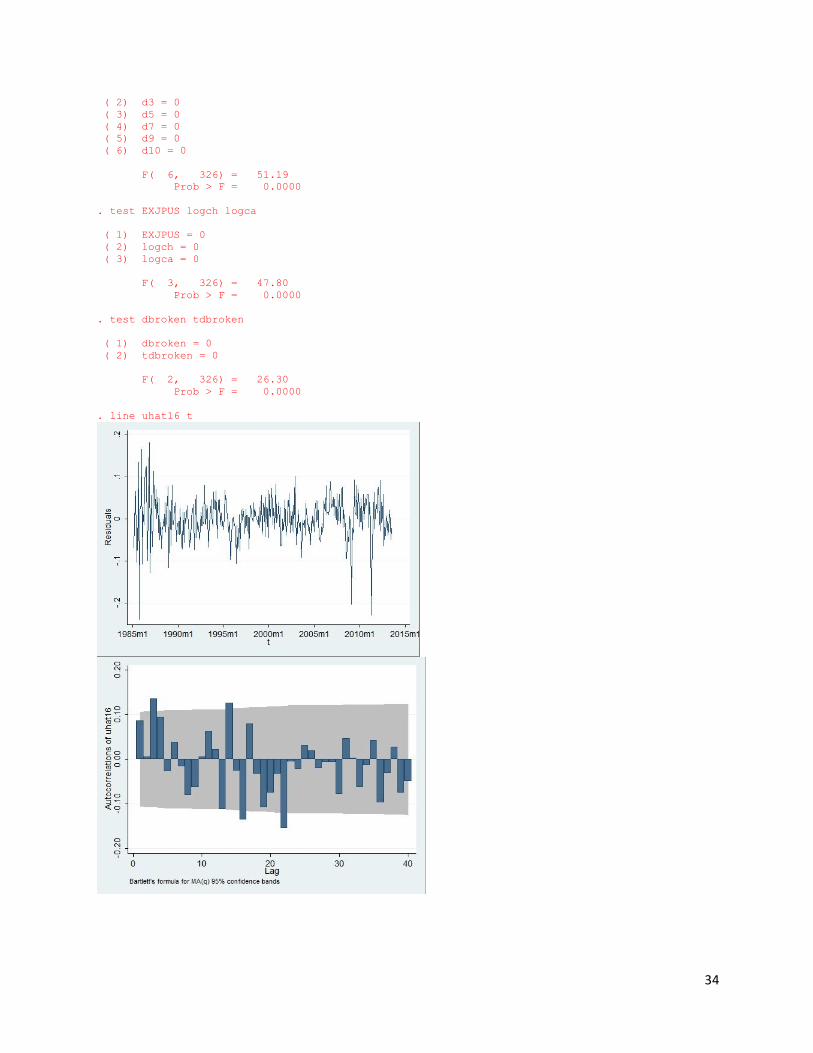
SECOND ONE reg logjp t dbroken tdbroken logch logca EXJPUS d1 d3 d5 d7 d9 d10 l(1/2).log > jp Source | SS df MS Number of obs = 341 -------------+------------------------------ F( 14, 326) = 387.91 Model | 14.5080484 14 1.03628917 Prob > F = 0.0000 Residual | .870903647 326 .002671484 R-squared = 0.9434 -------------+------------------------------ Adj R-squared = 0.9409 Total | 15.3789521 340 .045232212 Root MSE = .05169 ------------------------------------------------------------------------------ logjp | Coef. Std. Err. t P>|t| [95% Conf. Interval] -------------+---------------------------------------------------------------- t | -.0025757 .0003077 -8.37 0.000 -.0031809 -.0019704 dbroken | -2.214246 .3506743 -6.31 0.000 -2.904116 -1.524376 tdbroken | .0036834 .0005665 6.50 0.000 .0025689 .0047979 logch | .0870767 .0186327 4.67 0.000 .0504212 .1237322 logca | .3514477 .0366415 9.59 0.000 .2793641 .4235313 EXJPUS | -.0008258 .0001952 -4.23 0.000 -.0012098 -.0004418 d1 | -.0811049 .010684 -7.59 0.000 -.1021233 -.0600866 d3 | .0856687 .0116572 7.35 0.000 .0627358 .1086015 d5 | -.1060958 .0107366 -9.88 0.000 -.1272175 -.084974 d7 | .0582106 .0115275 5.05 0.000 .035533 .0808883 d9 | -.0515062 .0109438 -4.71 0.000 -.0730354 -.0299769 d10 | .0512363 .0113855 4.50 0.000 .028838 .0736345 | logjp | L1. | .3073899 .0383247 8.02 0.000 .231995 .3827849 L2. | .1780152 .0386042 4.61 0.000 .1020704 .2539601 | _cons | 1.916725 .3313809 5.78 0.000 1.26481 2.56864 ------------------------------------------------------------------------------ . estat ic ----------------------------------------------------------------------------- Model | Obs ll(null) ll(model) df AIC BIC -------------+--------------------------------------------------------------- . | 341 44.50145 534.0451 15 -1038.09 -980.612 ----------------------------------------------------------------------------- Note: N=Obs used in calculating BIC; see [R] BIC note . predict logjphat16 (option xb assumed; fitted values) (2 missing values generated) . predict uhat16,resid (2 missing values generated) . ac uhat16,recast(bar) . pac uhat16,recast(bar) . test l1.logjp logjpl2.logjp logjpl2: operator invalid r(198); . test l1.logjp l2.logjp ( 1) L.logjp = 0 ( 2) L2.logjp = 0 F( 2, 326) = 63.31 Prob > F = 0.0000 . test d1 d3 d5 d7 d9 d10 ( 1) d1 = 0

34

( 2) d3 = 0 ( 3) d5 = 0 ( 4) d7 = 0 ( 5) d9 = 0 ( 6) d10 = 0 F( 6, 326) = 51.19 Prob > F = 0.0000 . test EXJPUS logch logca ( 1) EXJPUS = 0 ( 2) logch = 0 ( 3) logca = 0 F( 3, 326) = 47.80 Prob > F = 0.0000 . test dbroken tdbroken ( 1) dbroken = 0 ( 2) tdbroken = 0 F( 2, 326) = 26.30 Prob > F = 0.0000 . line uhat16 t

35

ADL MODEL . reg dlogjp l(1/3) dlogjp l(1/2) EXJPUS,r Linear regression Number of obs = 339 F( 5, 333) = 18.45 Prob > F = 0.0000 R-squared = 0.2962 Root MSE = .07943 ------------------------------------------------------------------------------ | Robust dlogjp | Coef. Std. Err. t P>|t| [95% Conf. Interval] -------------+---------------------------------------------------------------- dlogjp | L1. | -.4973408 .0654322 -7.60 0.000 -.6260534 -.3686283 L2. | -.507811 .0591536 -8.58 0.000 -.624173 -.3914491 L3. | -.2705898 .0636974 -4.25 0.000 -.3958898 -.1452899 | EXJPUS | L1. | -.0043494 .0013624 -3.19 0.002 -.0070294 -.0016695 L2. | .004302 .0012842 3.35 0.001 .0017758 .0068282 | _cons | .0084736 .0225715 0.38 0.708 -.0359271 .0528743 ------------------------------------------------------------------------------ . test l1.EXJPUS l2.EXJPUS ( 1) L.EXJPUS = 0 ( 2) L2.EXJPUS = 0 F( 2, 333) = 6.15 Prob > F = 0.0024 . estat ic ----------------------------------------------------------------------------- Model | Obs ll(null) ll(model) df AIC BIC -------------+--------------------------------------------------------------- . | 339 321.1047 380.6355 6 -749.271 -726.315 ----------------------------------------------------------------------------- Note: N=Obs used in calculating BIC; see [R] BIC note . sum Variable | Obs Mean Std. Dev. Min Max -------------+--------------------------------------------------------

36

date | 343 14335.74 3018.178 9132 19540 EXJPUS | 343 119.9646 30.69057 76.643 260.4778 IMPCA | 343 15909.59 7604.686 4813.7 32208.4 IMPCH | 343 11875.27 11890.52 264.9 40252.1 IMPJP | 343 9684.725 1969.073 4799.8 14064.8 -------------+-------------------------------------------------------- SP500 | 343 851.2018 440.6646 167.24 1630.74 logjp | 343 9.155956 .2166855 8.47633 9.551431 logch | 343 8.616768 1.448115 5.579352 10.60292 logca | 343 9.542481 .5372161 8.479221 10.37998 logex | 343 4.760425 .2232936 4.339158 5.562518 -------------+-------------------------------------------------------- logsp500 | 343 6.566968 .6490371 5.11943 7.396789 t | 343 471 99.1598 300 642 jphat | 343 9684.725 1452.346 7180.169 12189.28 uhat | 343 2.14e-06 1329.639 -5311.955 4116.438 t2 | 343 231645 93820.42 90000 412164 -------------+-------------------------------------------------------- jphat2 | 343 9684.725 1595.516 5718.074 11135.15 uhat2 | 343 8.37e-07 1153.94 -4948.104 3403.33 logjphat3 | 343 9.155956 .180864 8.693827 9.317929 uhat3 | 343 -1.65e-10 .1193349 -.5817578 .2757282 dbroken | 343 .1574344 .3647419 0 1 -------------+-------------------------------------------------------- tdbroken | 343 96.90087 224.5841 0 642 logjphat4 | 343 9.155956 .1864987 8.81518 9.490631 uhat4 | 343 -8.28e-11 .1103215 -.4583945 .309154 d1 | 343 .0845481 .2786145 0 1 d2 | 343 .0845481 .2786145 0 1 -------------+-------------------------------------------------------- d3 | 343 .0845481 .2786145 0 1 d4 | 343 .0845481 .2786145 0 1 d5 | 343 .0845481 .2786145 0 1 d6 | 343 .0845481 .2786145 0 1 d7 | 343 .0845481 .2786145 0 1 -------------+-------------------------------------------------------- d8 | 343 .0816327 .2742042 0 1 d9 | 343 .0816327 .2742042 0 1 d10 | 343 .0816327 .2742042 0 1 d11 | 343 .0816327 .2742042 0 1 logjphat5 | 343 9.155956 .1928247 8.732186 9.540278 -------------+-------------------------------------------------------- uhat5 | 343 -1.08e-10 .0988494 -.3738964 .2419742 logjphat6 | 343 9.155956 .1923962 8.732051 9.540403 uhat6 | 343 1.08e-10 .099681 -.3740163 .241992 dbroken1 | 343 .2478134 .4323736 0 1 tdbroken1 | 343 135.3061 236.3927 0 588 -------------+-------------------------------------------------------- logjphat7 | 343 9.155956 .1944983 8.74509 9.490631 uhat7 | 343 -9.47e-11 .0955145 -.4401104 .2364402 logjphat8 | 343 9.155956 .2001311 8.66781 9.527825 uhat8 | 343 9.52e-11 .0830671 -.3609526 .2073348 logjphat9 | 343 9.155956 .2011525 8.625671 9.525499 -------------+-------------------------------------------------------- uhat9 | 343 3.75e-11 .0805623 -.3009698 .2284254 logjphat10 | 343 9.155956 .1955368 8.702657 9.48842 uhat10 | 343 1.99e-10 .09337 -.3800131 .2410841 logjphat12 | 343 9.155956 .1937228 8.689026 9.486425 uhat12 | 343 6.76e-11 .0970777 -.3322407 .2639617 -------------+-------------------------------------------------------- uhat13 | 343 3.24e-11 .0802033 -.300546 .2101141 logjphat14 | 340 9.160793 .2032293 8.580007 9.515034 uhat14 | 340 1.28e-10 .0574792 -.3375591 .2200721 logjphat15 | 341 9.159303 .2058914 8.578844 9.531652 uhat15 | 341 -9.42e-11 .0533004 -.2686388 .1800863 -------------+-------------------------------------------------------- logjphat16 | 341 9.159303 .206569 8.585711 9.494652 uhat16 | 341 1.81e-11 .0506111 -.2395513 .1817592 dlogjp | 342 .002035 .094809 -.355257 .2374716

37

Appendix C

For the group paper, we set our group meetings twice regularly from the beginning of the

semester to the due date of the final draft to share the ideas and work we have done independently,

discuss potential problems during the research, and combine the thoughts and works together to

build our final draft. We made three appointments with our instructor to discuss the questions we

may have about the paper and got the feedbacks from her. We visited the ESL writing center two

times for help during the semester. We went to Emory Electronic Data Center before the spring

break to find help for collecting data. We divided our work specifically to each group member: Kaidi

focused on the data collecting and analysis, Dayi focused on interpreting the data and regression

model by using real world experience and writing the major part of the paper, and Fanyu mainly

considered the structure and grammar of the paper and the data forecasting part.

422 final project

Documents