4D-PIV advances to visualize sound generation by air flows

Fulvio Scarano

Delft University of TechnologyAerospace Engineering Department – Aerodynamics Sectionf.scarano@tudelft.nl

Aero-acoustics Investigation approaches, from lab scale detail to full scale systems

Phased microphone arrayfield measurements (Sijtsma, DLR)

Phased microphone array in large wind tunnel (DNW)

Direct numerical simulation of a transitional jet (Freund et al. 2000)

Direct numerical simulation of trailing edge noise (DLR)

Jet noise prediction based on PIV and acoustic analogy (Schram, 2003, VKI)

Rod-airfoil noise prediction based on time-resolved PIV and Curle’s acoustic analogy

(Lorenzoni et al, 2008, TU Delft)

Aeroacoustics research approaches

Sound in the far-field by phase-microphones array(field tests and large-anechoic wind tunnels)

Phenomenological research by Computational aero-acoustics (CAA) - DNS, LES (direct approaches) - DNS+LEE, LES+BEM, RANS+SNGR (hybrid approaches)

Surface pressure sensors and acoustic analogiese.g. Pressure transducers and Curle analogy

Experimental noise-source identification by PIVstatistical techniques (spatio-temporal velocity correlations)time-resolved analysis (velocity or derived pressure spectra)

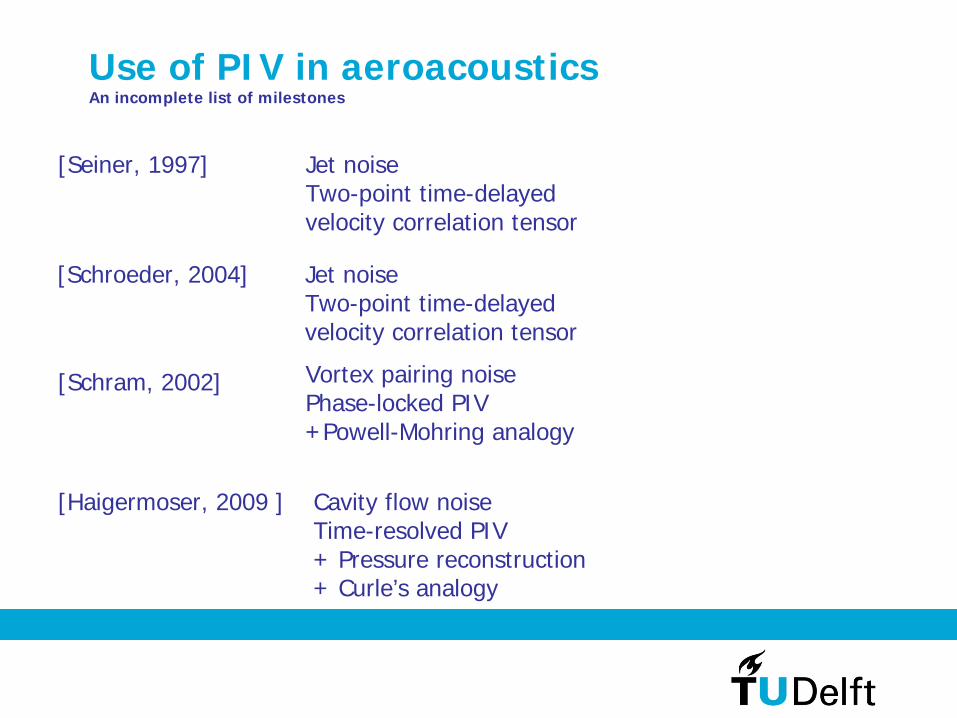
Use of PIV in aeroacoustics An incomplete list of milestones

Cavity flow noiseTime-resolved PIV+ Pressure reconstruction+ Curle’s analogy

Jet noiseTwo-point time-delayed velocity correlation tensor

Vortex pairing noisePhase-locked PIV+Powell-Mohring analogy

[Seiner, 1997]

[Schram, 2002]

[Haigermoser, 2009 ]

Jet noiseTwo-point time-delayed velocity correlation tensor

[Schroeder, 2004]

PIV and acoustic analogies Quantitative source visualization for noise prediction

Lighthill analogy (low Mach, far-field), e.g. Jet noise

Curle analogy (low Mach, far-field), e.g. Airframe noise

Gutin’s principle (dipolar term for compact rigid body)

In the use of analogies, the acoustic pressure p' is expressed as integral of the fluid dynamic properties in the source region

Vortex-structure interaction noise Acoustic source determination by time-resolved measurements

High-speed PIV and acoustic experiments (KAT-NLR) Illumination and imaging

2C TR-PIV : V (x,y,t)(2000x1000 pixels@2700Hz)

Planar Pressure Imaging (PPI): P (x,y,t) -> on airfoil surf

Curle’s analogy: p’ (x,y,t) (far field)

Acoustic array and far-field microphones

Data reduction

Planar Pressure Imaging (PPI) From time-resolved velocity field to the pressure spatial distribution

• Pressure gradient derived from experimental velocity data using definition of material derivative [Liu & Katz, 2006]:

• 2D Poisson equation for the pressure

• Incompressible and inviscid flow assumptions. Pressure solver [de Kat et al. 2008]. Neumann conditions at body surface. Dirichlet conditions in potential-flow region (e.g. free-stream).

Planar and surface pressure distribution Surface pressure fluctuations due to vortex interaction with airfoil LE

LE TE

η

r.m.s of pressure fluctuations along airfoil surface

vectors of velocity fluctuations

Planar pressure distribution (w.r.t. p∞

)

Assessment of PPI w.r.t. Direct surface pressure measurement (de Kat et al. 2008)

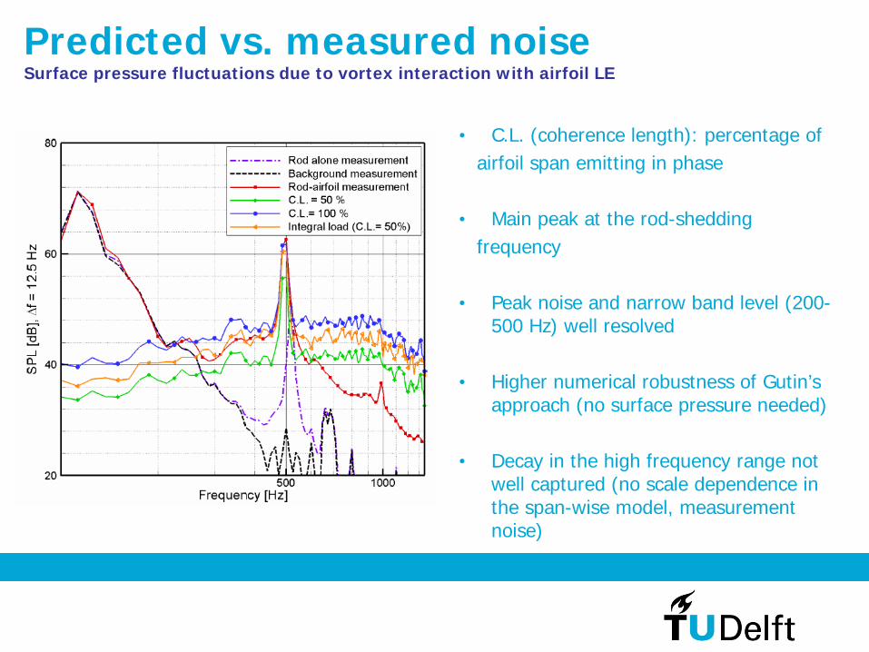
Predicted vs. measured noise Surface pressure fluctuations due to vortex interaction with airfoil LE

• C.L. (coherence length): percentage of airfoil span emitting in phase

• Main peak at the rod-shedding frequency

• Peak noise and narrow band level (200- 500 Hz) well resolved

• Higher numerical robustness of Gutin’s approach (no surface pressure needed)

• Decay in the high frequency range not well captured (no scale dependence in the span-wise model, measurement noise)

Emission directivity Surface pressure fluctuations due to vortex interaction with airfoil LE

- Maximum emission perpendicular to airfoil chord- emission 20% reduction in streamwise direction

Extension to 3D flow problems Vortex-based definitions of acoustic source

Lam

inar

flo

w a

t Re

= 3

60

Turb

ulen

t re

gim

e (R

e=

554

0)

Tom

ogra

phic

PIV

mea

sure

men

t

Dire

ct N

umer

ical

Sim

ulat

ion

3D PIV by tomography Elsinga et al. 2005 *

Computerized Axial Tomography (CAT)

Tomograpic PIV

particles in 3D space2d slice (tomos)

* Collaboration TU Delft – LaVision GmbH

Tomographic PIV Working principle: MART reconstruction and 3D cross-correlation

- Image to object 3D mapping function+Self calibration (Wieneke, 2008)

- Iterative volume reconstruction (Multiplicative Algebraic Reconstruction Technique, MART)

- 3D Cross-correlation (Volume Deformation Iterative MultiGrid, VODIM )

t t+ΔtA

B

C

D

3D intensity field3D velocity field

Digital images

Transitional Jets 4D-measurements by time-resolved tomographic PIV

Jet:Nozzle exit diameter: 10 mmExit velocity: 0.1 – 2.5 m/sRe: 1,500 – 25,000Simulation domain: up to 60 diameters

Measurement equipment:Quantronix Darwin-Duo: 2x25 mJ@1kHz4xPhotron SA1: 1024x1024@5.4kHzLatex particles: C~0.8 part/mm3

Data analysis:LaVision DaVis7.4Meas. domain (cylindrical): 2x2x5 D3

Box size: 1.5x1.5x1.5 mm3

Time resolution: ~20 samples/cycle

Jet tomography facility

Planar PIV illumination

Transitional Jets 4D-measurements by time-resolved tomographic PIV

( ) ( ) 30' ,

SV

p t G dyρ= × ∇∫x ω V

Powell analogy

- Far field acoustic prediction-

Comparison with incompressible DNS

- Acoustic measurements in air jet under similarity conditions

ConclusionsTime resolved PIV enabling planar pressure field imaging (PPI)

PIV used with Curle’s analogy for the prediction of rod-airfoil acoustics

Introduction of tomographic PIV for the 3D complex flows 3D vorticity patterns of transitional and turbulent flows

Time-resolved tomo-PIV for acoustic source analysis Jet noise prediction by means of 4D-PIV and Powell’s analogy

Congratulations to DLR successful 25 years in PIV

…and best wishes for the next 25!!!