4th meeting of the scientific committee · 4th meeting of the scientific committee the hague,...
TRANSCRIPT

4th Meeting of the Scientific Committee
The Hague, Kingdom of the Netherlands 10 - 15 October 2016
SC-04-26
Notes on Peruvian Experience on Acoustic Data Collection Mariano Gutiérrez, Cynthia Vasquez, Salvador Peraltilla, Anibal Aliaga, Alex
Zuzunaga, Emilio Mendez, Edwin Yarlequé, Ulises Munaylla

1
South Pacific Regional Fisheries Management Organization 4th Scientific Committee 2016
Sociedad Nacional de Pesqueria - SNP
Notes on the Peruvian experience on acoustic data collection and quantitative analysis of fish and macro zooplankton habitat using industry vessels
Mariano Gutiérrez1, Cynthia Vasquez1, Salvador Peraltilla2, Anibal Aliaga3, Alex Zuzunaga4, Emilio
Mendez5, Edwin Yarlequé6, Jeremie Habasque7, Ulises Munaylla8
1. Introduction Peruvian industry has contributed information and proposals of analysis of data collected by fishing vessels since the early days of SPRFMO. The focus has been the Pacific Jack Mackerel (PJM) stock assessment through acoustic methods used aboard fishing vessels as the best and cheaper alternative to slow and expensive conventional acoustic surveying. New methods of analysis evolved in Peru to offer additional information from the same data to get relative abundance indexes of macro zooplankton, the detection of oxycline location and the upper limit of the oxygen minimum zone (ULOMZ), the detection of internal waves and convergent or divergent processes, the vertical migration of fish and plankton, and the calculation of the volume of the pelagic habitat. In this document we review notes on recent achievements not necessarily linked to PJM but a methodology improvement as a contribution to the SPRMO Scientific Working Group.
2. Calibration of Simrad ES60 echo sounders for fish biomass estimation aboard Fishing Vessels Fishing Companies responded positively in 2015 (October) and 2016 (May) the call from the Peruvian Marine Research Institute (IMARPE) to support the official development of joint acoustic assessments surveys of the abundance of small pelagic fish populations with emphasis in anchovy (Engraulis ringens) from 5 to 16°S (about 1,000 km or 540 n.mi. from 1 up to 100 km or 60 n.mi.) off shore. In the first case participated 11 fishing vessels (FV) and 6 FV in the second case, all of them deploying Kongsberg Simrad ES60 or ES70 echo sounders operating at 120 kHz with split beam transducers. Calibrations took place before the surveys in the vicinity of San Lorenzo Island, near Callao (12°S), also near Chimbote (9°S). A seventh small vessel of the industry participated in the second survey using a portable scientific echo sounder Kongsberg Simrad EY60 also at 120 kHz in order of surveying shallow waters areas. According to Demer et al (20159) ES60 and ES70 software packages do not include a calibration utility. Nevertheless, these echo sounders may be calibrated. This section outlines the calibration procedures that are unique to ES60 and ES70 echo sounders. A specific calibration protocol for fishing vessels deploying ES60 and ES70 systems have been delivered in 2015 to the SPRFMO Scientific Working Group (SWG) by the Fishing Vessels as Scientific Platforms Task Group (FVSP-TG).
1 Universidad Nacional Federico Villarreal, Lima, Perú 2 Tecnológica de Alimentos S.A. 3 Pesquera Diamante 4 Compañía Pesquera Inca 5 Austral Group 6 Pesquera Hayduk 7 Instituto de Investigación para el Desarrollo, Francia 8 Sociedad Nacional de Pesquería, Perú 9 Demer, D.A., Berger, L., Bernasconi, M., Bethke, E., Boswell, K., Chu, D., Domokos, R., et al. 2015. Calibration of acoustic instruments. ICES Cooperative Research Report No. 326. 133pp.

2
There are 3 ways of calibrating echo sounders as the ES60/70: (1) Using “Calibration.exe” routine from the ER60 software (Kongsberg Simrad) by using a sphere that is moved throughout the transducer beam; the steps are detailed in Simrad (200810). (2) Using “ExCal”, which is a free open-source11 Matlab (The Mathworks, MA, USA) script for estimating calibration parameters for EK60, ES60, and ES70 echo sounders; it reads raw data files obtained from the sphere. (3) Performing an “On-axis calibration”, which is made by using only the data when the sphere is positioned on the beam axis. This is most accurately accomplished using split-beam angle measurements to position the sphere and a post -processing application, e.g. Echoview (Echoview Software Pty Ltd), to filter the measurements and calculate mean 𝑆𝑎. In Peru the first and third methods have been used for calibrating the ES60/70 echo sounders; the third method is the one used in the FVSP-TG specific protocol. Furthermore the echo sounders were calibrated by calculating the theoretical value of nautical area scattering coefficient (Sa) of a sphere whose reflectivity (TS) is known. The methodology originated in the publications by Foote et al 198312 and 1987 (ICES Cooperative Research Report –CRR- 147), followed by a new and updated version by Demer et al 201513. In all cases they were used 21 mm diameter copper spheres (TS: Target Strength= -40.4 dB). The sphere was immersed using three nylon lines (Figure 1). Measured TS was compared to the nominal value to modify the gain value of the transducer (G).
Figure 1: Calibration arrangement of three nylon lines and a cupper sphere (redrawn from Simmonds
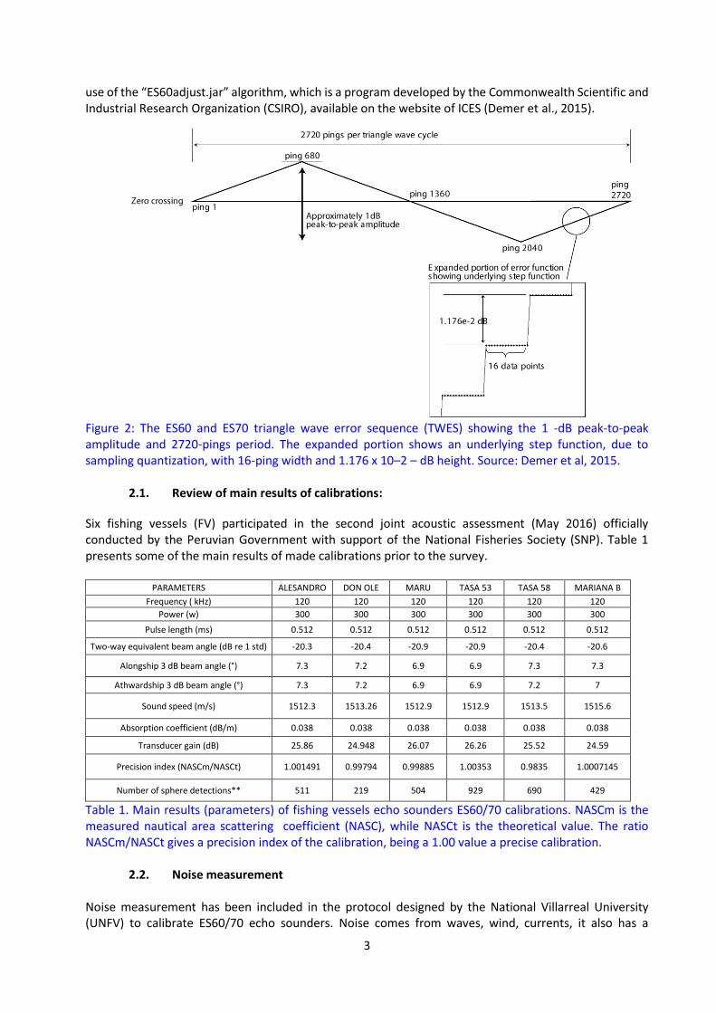
and MacLennan, 2005). The so-called triangular wave error contained in RAW files can affect the calibration, then the files has been corrected. The RAW files of the ES60 and ES70 systems are modulated by the software of the echo sounders with a sequence of triangular error wave (TWE: Triangle Wave Error) with a peak-to-peak amplitude of 1dB and a period of 2720-pings (Ryan and Kloser, 200414, figure 2). TWE averages are close to zero for a full period of the wave, so that its contribution to sampling error can be insignificant for large data sets. However, TWE can skew the results of calibration ± 0.5 dB. (Demer et al. 2015). Therefore, before performing any kind of analysis it should be removed the TWE from RAW files. This is achieved with the
10 Simrad. 2008. ER60 Scientific echo sounder software reference manual, Simrad Subsea A/S, Horten, Norway. 221 pp. 11 http://ices.dk/publications/Documents/Forms/AllItems.aspx 12Foote, K.G. (1983).Maintaining precision calibrations with optimal copper spheres.Journal of theAcoustical Society of America. 13 Demer, D.A., Berger, L., Bernasconi, M., Bethke, E., Boswell, K., Chu, D., Domokos, R., et al. 2015. Calibration of acoustic instruments. ICES Cooperative Research Report No. 326. 133pp. 14 Ryan T., R. Kloser. 2004. Quantification and correction of a systematic error in Simrad ES60 echo sounders. Technical Note, FAST ICES Working Group, Dansk, Poland. 9 pp.
3
use of the “ES60adjust.jar” algorithm, which is a program developed by the Commonwealth Scientific and Industrial Research Organization (CSIRO), available on the website of ICES (Demer et al., 2015).
Figure 2: The ES60 and ES70 triangle wave error sequence (TWES) showing the 1 -dB peak-to-peak amplitude and 2720-pings period. The expanded portion shows an underlying step function, due to sampling quantization, with 16-ping width and 1.176 x 10⁻² – dB height. Source: Demer et al, 2015.
2.1. Review of main results of calibrations:
Six fishing vessels (FV) participated in the second joint acoustic assessment (May 2016) officially conducted by the Peruvian Government with support of the National Fisheries Society (SNP). Table 1 presents some of the main results of made calibrations prior to the survey.
PARAMETERS ALESANDRO DON OLE MARU TASA 53 TASA 58 MARIANA B
Frequency ( kHz) 120 120 120 120 120 120
Power (w) 300 300 300 300 300 300
Pulse length (ms) 0.512 0.512 0.512 0.512 0.512 0.512
Two-way equivalent beam angle (dB re 1 std) -20.3 -20.4 -20.9 -20.9 -20.4 -20.6
Alongship 3 dB beam angle (°) 7.3 7.2 6.9 6.9 7.3 7.3
Athwardship 3 dB beam angle (°) 7.3 7.2 6.9 6.9 7.2 7
Sound speed (m/s) 1512.3 1513.26 1512.9 1512.9 1513.5 1515.6
Absorption coefficient (dB/m) 0.038 0.038 0.038 0.038 0.038 0.038
Transducer gain (dB) 25.86 24.948 26.07 26.26 25.52 24.59
Precision index (NASCm/NASCt) 1.001491 0.99794 0.99885 1.00353 0.9835 1.0007145
Number of sphere detections** 511 219 504 929 690 429
Table 1. Main results (parameters) of fishing vessels echo sounders ES60/70 calibrations. NASCm is the measured nautical area scattering coefficient (NASC), while NASCt is the theoretical value. The ratio NASCm/NASCt gives a precision index of the calibration, being a 1.00 value a precise calibration.
2.2. Noise measurement Noise measurement has been included in the protocol designed by the National Villarreal University (UNFV) to calibrate ES60/70 echo sounders. Noise comes from waves, wind, currents, it also has a
4
biological origin, and also the noise is generated by boat (engine, propeller, vibration, cavitation). Many of these noises are observable in an echogram. The noise measurements must ideally be perform to a depth of 200 m or deeper, and in conditions of low transit and calm sea. To be able to remove noise from echograms it is necessary to measure it for every vessel. Therefore all echosounders were operated in passive mode. NASC values were measured for the first meter from the transducer at several boat speeds, from 0 to the maximum, in different courses when possible. The estimation of the maximum tolerable noise level (NL) was suggested by ICES (Mitson R. et al. 199515): 𝑁𝐿 = 130 − 22𝑙𝑜𝑔𝑓, where f is the used frequency. NL can also be calculated from the backscattered values (Sv): 𝑁𝐿 = 𝑃𝑁 − 20𝑙𝑜𝑔𝜆 − 𝐺 + 192.8 PN is the mean backscattered volume (dB) by used intervals, λ (Hz) is the wave length (cm) obtained by dividing the sound speed per second (C, in m/s) and the frequency (λ =C/f). G is the transducer gain (dB).
2.3. Algorithm for noise reduction, removal of interferences, and detection of ULOMZ,
macrozooplankton and fish
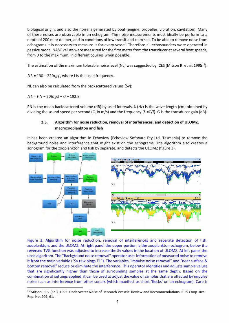
It has been created an algorithm in Echoview (Echoview Software Pty Ltd, Tasmania) to remove the background noise and interference that might exist on the echograms. The algorithm also creates a sonogram for the zooplankton and fish by separate, and detects the ULOMZ (figure 3).
Figure 3. Algorithm for noise reduction, removal of interferences and separate detection of fish, zooplankton, and the ULOMZ. At right panel the upper portion is the zooplankton echogram; below it a reversed TVG function was adjusted to increase the Sv values in the location of ULOMZ. At left panel the used algorithm. The "Background noise removal" operator uses information of measured noise to remove it from the main variable ("Sv raw pings T1"). The variables "impulse noise removal" and "near surface & bottom removal" reduce or eliminate the interference. This operator identifies and adjusts sample values that are significantly higher than those of surrounding samples at the same depth. Based on the combination of settings applied, it can be used to adjust the value of samples that are affected by impulse noise such as interference from other sonars (which manifest as short ‘flecks’ on an echogram). Care is
15 Mitson, R.B. (Ed.), 1995. Underwater Noise of Research Vessels: Review and Recommendations. ICES Coop. Res. Rep. No. 209, 61.
5
required to prevent it from adjusting good data. The operator is based on the “impulsive noise (IN)” algorithm and definitions described in Ryan et al. (2015). The operators “TVG” and “plankton=TVG” vertically invert the TVG function and add it to the zooplankton values in order to get the higher values at the base line of the ULOMZ. The variables “OMZ” and “OMZ smoothed” detect the ULOMZ. The variable “fish” is obtained by subtracting the variable “near surface & bottom removal” from the variable “plankton thresholding method” using as a practical Sv a threshold limit of -65 dB. The algorithm was developed in Echoview by M. Gutierrez (UNFV) and T. Jarbys (Echoview Software Pty Ltd).
3. Comparison of Sv and NASC values obtained by fishing vessels To compare the acoustic measurements obtained aboard several boats to check and validate their quantitative use, an experiment on echointegration was performed among FVs. Two groups of 3 vessels sailed with a distance separation between them from 30 and 50 m, in calm sea conditions at more than 180 m depth (100 fathoms 180 m) in order to reduce the reverberation that might affect the measurements. This comparison leaded to an intercalibration when one of those boats was not previously calibrated. The experiment was performed in two consecutive days (February 10 and 11 2016). The first group and day was formed by FRV Olaya and FVs Alessandro and Nueva Resbalosa. The second group and day was formed by FRV Olaya and FVs TASA 54 and TASA 56. The two days the groups sailed until 30 miles off shore. FRV Olaya deployed an EK60 scientific echosounder, all the other deployed ES60/70 systems.
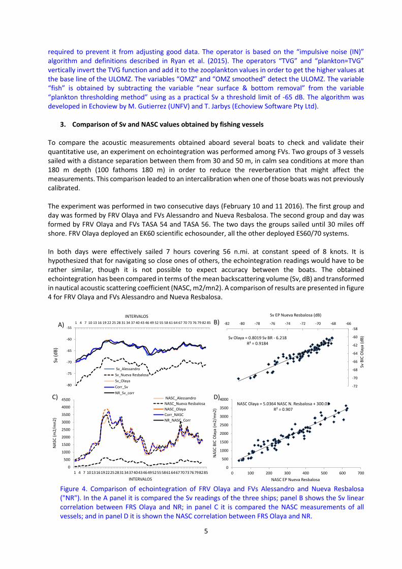
In both days were effectively sailed 7 hours covering 56 n.mi. at constant speed of 8 knots. It is hypothesized that for navigating so close ones of others, the echointegration readings would have to be rather similar, though it is not possible to expect accuracy between the boats. The obtained echointegration has been compared in terms of the mean backscattering volume (Sv, dB) and transformed in nautical acoustic scattering coefficient (NASC, m2/mn2). A comparison of results are presented in figure 4 for FRV Olaya and FVs Alessandro and Nueva Resbalosa.
Figure 4. Comparison of echointegration of FRV Olaya and FVs Alessandro and Nueva Resbalosa ("NR"). In the A panel it is compared the Sv readings of the three ships; panel B shows the Sv linear correlation between FRS Olaya and NR; in panel C it is compared the NASC measurements of all vessels; and in panel D it is shown the NASC correlation between FRS Olaya and NR.
-80
-75
-70
-65
-60
-55
1 4 7 10 13 16 19 22 25 28 31 34 37 40 43 46 49 52 55 58 61 64 67 70 73 76 79 82 85
Sv (
dB
)
INTERVALOS
Sv_Alessandro
Sv_Nueva Resbalosa
Sv_Olaya
Corr_Sv
NR_Sv_corr
0
500
1000
1500
2000
2500
3000
3500
4000
4500
1 4 7 1013161922252831343740434649525558616467707376798285
NA
SC (
m2
/mn
2)
INTERVALOS
NASC_Alessandro
NASC_Nueva Resbalosa
NASC_Olaya
Corr_NASC
NR_NASC_Corr
Sv Olaya = 0.8019 Sv BR - 6.218R² = 0.9184
-72
-70
-68
-66
-64
-62
-60
-58
-82 -80 -78 -76 -74 -72 -70 -68 -66
Sv B
IC O
laya
(d
B)
Sv EP Nueva Resbalosa (dB)
NASC Olaya = 5.0364 NASC N. Resbalosa + 300.03R² = 0.907
0
500
1000
1500
2000
2500
3000
3500
4000
0 100 200 300 400 500 600 700
NA
SC B
IC O
laya
(m
2/m
n2
)
NASC EP Nueva Resbalosa
A) B)
C) D)

6
FRV Olaya and FV Alessandro were calibrated before the experiment, not so the FV Nueva Resbalosa. Figure 4-A shows the correspondence of Sv values of FRV Olaya and FV Alessandro; in the same panel FV Nueva Resbalosa appears with a difference of 10 dB or less due to the fact that it was not previously calibrated. Therefore a correlation analysis was made for correcting the FV Nueva Resbalosa values. It was found a significant Pearson correlation (0.91). The same approach was tested for NASC values (0.90), which is checked in panel 4B to 4D. This demonstrate two aspects: scientific echosounder (EK60) is compatible with ES60/70 systems, and there is a possibility of using data even from no calibrated vessels if an acoustic correlation between acoustic measurements is found. Figure 5 shows similar analysis for the case of FRV Olaya compared to FVs TASA 56 and TASA 54. FRV Olaya and FV TASA 56 were calibrated prior to the experiment, not so the FV TASA 54. Figure 5-A shows the coincidence of Sv readings among FRV Olaya and FV TASA 56. Sv readings of FV TASA 54 appears with 3 dB or less. To analyze if it is still possible to use FV TASA 54 data an analysis of its correlation with Sv readings from FRV Olaya was done. It was found a significant Pearson correlation (0.80). Also it was tested the NASC correlation (0.86) among the two vessels. Panels 5A to 5D shows the made comparison and correlations found.
Figure 5. Comparison of echointegration measured by FRV Olaya and FVs TASA 56 and TASA 54. A panel compares the Sv readings of the three ships; panel B shows the correlation between the measurements of FRV Olaya and FV TASA 54, panel C compare the NASC values of the 3 vessels, and panel D shows the correlation between FRV Olaya and FV TASA 54. In conclusion, the echointegration readings are compatible and comparable among scientific and commercial models of Simrad echosounders. The manufacturer and the employed frequency (120 kHz) are similar, which demonstrates that it is possible to perform acoustic assessments using the echo sounders currently installed on board some ships of the fleet. In other words, the quantitative use of acoustic dada does not depends on of the boat but on having made proper calibration of the instruments. Also, this experiment shows that a not calibrated echo sounder still can generate useful information if it is subjected to an intercalibration as it has been proven in those exposed cases. The comparison of the echointegrated values, in terms of mean backscattered volume (Sv, dB) and nautical area scattering coefficients (NASC, in m2/mn2) for FRV Olaya and FVs Alessandro and Nueva Resbalosa are appreciated in figure 6.
-75
-73
-71
-69
-67
-65
-63
-61
1 6 11
16
21
26
31
36
41
46
51
56
61
66
71
76
81
86
91
96
10
1
10
6
11
1
Sv (
dB
)
INTERVALOS
Sv_Tasa56
Sv_Tasa54
Sv_Olaya
Corr_Sv
Tasa54_Sv_corr
Sv Olaya = 0.7738 Sv Tasa 54 - 13.273R² = 0.8022
-70
-68
-66
-64
-62
-60
-58
-75 -70 -65 -60
Sv B
IC IO
laya
(d
B)
Sv EP Tasa 54
NASC Olaya = 1.1765 NASC Tasa 54 + 282.28R² = 0.8666
0
500
1000
1500
2000
2500
3000
3500
4000
0 1000 2000 3000 4000
NA
SC B
IC O
laya
(m
2/m
n2
)
NASC EP Tasa 54
0
500
1000
1500
2000
2500
3000
3500
4000
4500
5000
1 6
11
16
21
26
31
36
41
46
51
56
61
66
71
76
81
86
91
96
10
1
10
6
11
1
NA
SC (
m2
/mn
2)
INTERVALO
Corr_NASC
NASC_Olaya
NASC_Tasa56
NASC_Tasa54
Tasa54_NASC_Corr
A)B)
C)D)

7
Figure 6. Compared distribution of mean backscattered volume (Sv, dB, top panel) and nautical area scattering coefficient (NASC, in m2/mn2, bottom panel) for FRV Olaya and FVs Alessandro and Nueva Resbalosa.
Higher values of echointegration can be seen in the upper quadrant of each panel in all of the cases shown in Figure 6, and lower values at the bottom. Altogether these acoustic values represent the total echointegration between fish and zooplankton in the area where the experiment took place. Results have been statistically analyzed, it is concluded that no significant differences exist between measurements obtained between the 3 vessels (table 2). Table 2 presents that there is no difference in echointegration (Sv or NASC), which demonstrate the compatibility of measurements. It is concluded that the use of a similar acoustic instrument offers reliable measurements independently of the ship in which it is installed the calibrated echosounder. Table 2. Summary of compared statistics between FRV Olaya (used as a reference) and the average of the fishing vessels (FVs) Alessandro and Nueva Resbalosa. The column Data FRV Olaya refers to values measured by a scientific echo sounder (EK60), the column Data FVs refers to the mean values obtained by FVs using ES60/70 systems. The column Residuals presents the difference between FRV Olaya and the FVs. The last column shows the difference in percentages.
Statistics Data FRV Olaya Data FVs Residuals Percentage
Standard deviation Sv (dB): 2.38 2.10 0.28 11.79
Maximum Sv (dB): -60.18 -60.77 0.59 0.98
Minimum Sv (dB): -70.15 -69.60 -0.55 0.78
Average Sv (dB): -63.34 -63.43 0.09 0.14
Standard deviation NASC (m2/mn2): 849.64 762.23 87.41 10.29
Maximum NASC (m2/mn2): 3,888.61 3,398.93 489.68 12.59
Minimum NASC (m2/mn2): 391.34 451.84 -60.50 15.46
Average NASC (m2/mn2): 1,875.76 1,840.29 35.48 1.89
The comparison of the echointegrated values, in terms of mean backscattered volume (Sv, dB) and nautical area scattering coefficients (NASC, in m2/mn2) for FRV Olaya and FVs TASA 56 and TASA 54 are appreciated in figure 7.
Sv (
dB
)N
ASC
(m
2 /m
n2 )
Sv Alessandro Sv Olaya Sv Nueva Resbalosa
NASC Alessandro NASC Olaya NASC Nueva Resbalosa
8
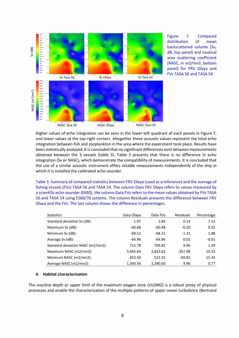
Figure 7. Compared distribution of mean backscattered volume (Sv, dB, top panel) and nautical area scattering coefficient (NASC, in m2/mn2, bottom panel) for FRV Olaya and FVs TASA 56 and TASA 54.
Higher values of echo integration can be seen in the lower-left quadrant of each panels in Figure 7, and lower values at the top-right corners. Altogether these acoustic values represent the total echo integration between fish and zooplankton in the area where the experiment took place. Results have been statistically analyzed. It is concluded that no significant differences exist between measurements obtained between the 3 vessels (table 3). Table 3 presents that there is no difference in echo integration (Sv or NASC), which demonstrate the compatibility of measurements. It is concluded that the use of a similar acoustic instrument offers reliable measurements independently of the ship in which it is installed the calibrated echo sounder. Table 3. Summary of compared statistics between FRV Olaya (used as a reference) and the average of fishing vessels (FVs) TASA 56 and TASA 54. The column Data FRV Olaya refers to values measured by a scientific echo sounder (EK60), the column Data FVs refers to the mean values obtained by FVs TASA 56 and TASA 54 using ES60/70 systems. The column Residuals presents the difference between FRV Olaya and the FVs. The last column shows the difference in percentages.
Statistics Data Olaya Data FVs Residuals Percentage
Standard deviation Sv (dB): 1.97 1.83 0.14 7.13
Maximum Sv (dB): -60.68 -60.48 -0.20 0.32
Minimum Sv (dB): -69.52 -68.21 -1.31 1.88
Average Sv (dB): -64.96 -64.96 0.01 -0.01
Standard deviation NASC (m2/mn2): 715.78 705.82 9.96 1.39
Maximum NASC (m2/mn2): 3,465.64 3,823.62 -357.98 10.33
Minimum NASC (m2/mn2): 452.50 522.32 -69.82 15.43
Average NASC (m2/mn2): 1,300.56 1,290.60 9.96 0.77
4. Habitat characterization
The oxycline depth or upper limit of the maximum oxygen zone (ULOMZ) is a robust proxy of physical processes and enable the characterization of the multiple patterns of upper ocean turbulence (Bertrand
Sv Tasa 56 Sv Olaya
Sv (
dB
)
Sv Tasa 54
NASC Tasa 56
NA
SC (
m2/m
n2)
NASC Olaya NASC Tasa 54

9
et al., 201016, 201417). We acoustically estimated oxycline depth (Fig. 8) throughout a specific protocol to analyze and reveal submesoscale (kms) to mesoscale (tens of kms) features (figure 3). To probe this we used acoustic data collected by the fleet during summer 2011 during the pacific jack mackerel (PJM) fishing season.
Figure 8. From estimated (left panel) to interpolated (right panel) oxycline depth using acoustic data of 19 fishing trips done by TASA vessels (January 2011). Results show that the oxycline was superficial along the coastline and deeper off Callao (~12°S). Mean sea level anomaly (MSLA) measured over the same period shows an anticyclonic eddie South to 12°S (Fig. 9). If the eddies’ heart is in surface associated to a pycnocline deepening, that can explain the observed deeper oxycline.
Figure 9. Mean Sea Level Anomaly (MSLA) from January 6 to January 31, 2011 and tracks of TASA fishing trips during which acoustic data was collected January 6 to January 31, 2011 Thus we considered that the proposed protocol is correct at mesoscale (10-50 km) though we admit that there are «uncertain» sequences at sub-mesoscale (<10km). However the proposed method allows high
16 Bertrand, A., Ballon, M., and Chaigneau, A. (2010). Acoustic observation of living organisms reveals the upper limit of the oxygen minimum zone. PloS One 5, p. e10330 17 Bertrand, A., Grados, D., Colas, F., Bertrand, S., Capet, X., Chaigneau, A., Vargas, G., Mousseigne, A., and Fablet, R. (2014). Broad impacts of fine-scale dynamics on seascape structure from zooplankton to seabirds. Nature Communications 5

10
resolution time space monitoring of the ULOMZ. It can be easily implemented on any vessel equipped with acoustic echo sounders. The vertical distribution of forage fish strongly affects their catchability by animal predators and fishers.
4.1. Shoal spatial distribution
Horizontal distribution of fish schools is shown on Figure 10.
Figure 10. Spatial distribution of schools, size represents relative length of fish schools; color represents acoustic density (mean volume of backscattered strength, MVBS) Positions, morphological dimensions (height, length) and energetic parameters of schools are extracted from the fishing trips data (Table 1). Day and night information is presented separately. Sampled area clearly indicates a large day–night difference in schools vertical distribution. Table 1. Main characteristics of schools (PJM and mackerel)
Characteristics Day Night Total
Number of shoals 1465 1840 3305 Depth mean (m) 39 17 Length mean (m) 80 88 Height mean (m) 7 8 MVBS mean (dB) -53 -54
Species identification and biomass calculation is possible when proper catch data and biological sampling exist. This has been done during 6 SNP workshops performed during 2010-15. Biomass of PJM was acoustically calculated based on NASC values registered. However, Vargas (201418) sustain that many times the echo sounder does not detect fish but a positive catch (using purse seines in all cases) was obtained. This effect only can be explained by avoidance reaction of PJM in the presence of fishing vessels. Nevertheless during 2011 there were made weekly acoustic biomass calculations, with calculated biomass in a range of 300 to 600 thousand tonnes in the area explored by the fleet.
18 Vargas G. (2013). Localization of fishing grounds for the Peruvian fishing fleet using acoustics and geostatistics methods. Thesis. Universidad Nacional Federico Villarreal, 55 pp.
11
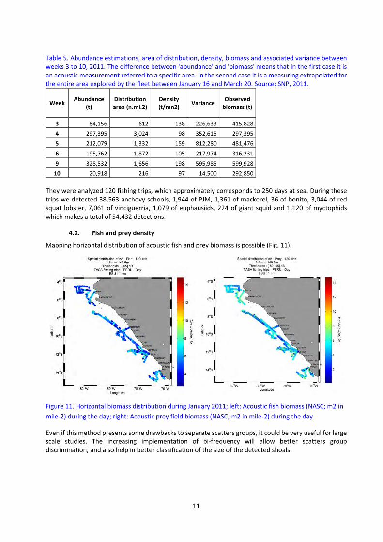
Table 5. Abundance estimations, area of distribution, density, biomass and associated variance between weeks 3 to 10, 2011. The difference between 'abundance' and 'biomass' means that in the first case it is an acoustic measurement referred to a specific area. In the second case it is a measuring extrapolated for the entire area explored by the fleet between January 16 and March 20. Source: SNP, 2011.
Week Abundance
(t) Distribution area (n.mi.2)
Density (t/mn2)
Variance Observed
biomass (t)
3 84,156 612 138 226,633 415,828
4 297,395 3,024 98 352,615 297,395
5 212,079 1,332 159 812,280 481,476
6 195,762 1,872 105 217,974 316,231
9 328,532 1,656 198 595,985 599,928
10 20,918 216 97 14,500 292,850
They were analyzed 120 fishing trips, which approximately corresponds to 250 days at sea. During these trips we detected 38,563 anchovy schools, 1,944 of PJM, 1,361 of mackerel, 36 of bonito, 3,044 of red squat lobster, 7,061 of vinciguerria, 1,079 of euphausiids, 224 of giant squid and 1,120 of myctophids which makes a total of 54,432 detections.
4.2. Fish and prey density
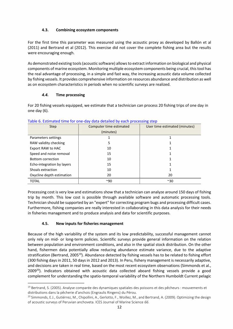
Mapping horizontal distribution of acoustic fish and prey biomass is possible (Fig. 11).
Figure 11. Horizontal biomass distribution during January 2011; left: Acoustic fish biomass (NASC; m2 in
mile-2) during the day; right: Acoustic prey field biomass (NASC; m2 in mile-2) during the day
Even if this method presents some drawbacks to separate scatters groups, it could be very useful for large scale studies. The increasing implementation of bi-frequency will allow better scatters group discrimination, and also help in better classification of the size of the detected shoals.
12
4.3. Combining ecosystem components
For the first time this parameter was measured using the acoustic proxy as developed by Ballón et al (2011) and Bertrand et al (2012). This exercise did not cover the complete fishing area but the results were encouraging enough. As demonstrated existing tools (acoustic software) allows to extract information on biological and physical components of marine ecosystem. Monitoring multiple ecosystem components being crucial, this tool has the real advantage of processing, in a simple and fast way, the increasing acoustic data volume collected by fishing vessels. It provides comprehensive information on resources abundance and distribution as well as on ecosystem characteristics in periods when no scientific surveys are realized.
4.4. Time processing For 20 fishing vessels equipped, we estimate that a technician can process 20 fishing trips of one day in one day (6). Table 6. Estimated time for one-day data detailed by each processing step
Step Computer time estimated
(minutes)
User time estimated (minutes)
Parameters settings 1 1
RAW validity checking 5 1
Export RAW to HAC 10 1
Speed and noise removal 15 1
Bottom correction 10 1
Echo-integration by layers 15 1
Shoals extraction 10 1
Oxycline depth estimation 20 20
TOTAL ~90 ~30
Processing cost is very low and estimations show that a technician can analyze around 150 days of fishing trip by month. This low cost is possible through available software and automatic processing tools. Technician should be supported by an "expert" for correcting program bugs and processing difficult cases. Furthermore, fishing companies are really interested in collaborating in this data analysis for their needs in fisheries management and to produce analysis and data for scientific purposes.
4.5. New inputs for fisheries management Because of the high variability of the system and its low predictability, successful management cannot only rely on mid- or long-term policies. Scientific surveys provide general information on the relation between population and environment conditions, and also in the spatial stock distribution. On the other hand, fishermen data potentially allow reducing abundance estimate variance, due to the adaptive stratification (Bertrand, 200519). Abundance detected by fishing vessels has to be related to fishing effort (300 fishing days in 2011, 50 days in 2012 and 2013). In Peru, fishery management is necessarily adaptive, and decisions are taken in real time, based on the most recent ecosystem observations (Simmonds et al., 200920). Indicators obtained with acoustic data collected aboard fishing vessels provide a good complement for understanding the spatio-temporal variability of the Northern Humboldt Current pelagic
19 Bertrand, S. (2005). Analyse comparée des dynamiques spatiales des poissons et des pêcheurs : mouvements et distributions dans la pêcherie d’anchois (Engraulis Ringens) du Pérou. 20 Simmonds, E.J., Gutiérrez, M., Chipollini, A., Gerlotto, F., Woillez, M., and Bertrand, A. (2009). Optimizing the design of acoustic surveys of Peruvian anchoveta. ICES Journal of Marine Science 66.

13
ecosystem. Modern fishing of small pelagic fish is mostly dependent on detection and location of fish shoals by acoustic instruments (Fréon et al., 200521). The scientific data collected by commercial fishing vessels in Peru have made, and will make, a significant contribution to understanding of the biology, distribution, movement and abundance of pelagic species relative to changing environmental parameters. Abundance estimates from scientific surveys could be dramatically improved when adding calibrated acoustic data from fishing vessels.
5. Some proposal on improvements to the used acoustic methods
5.1. Industry vessels surveys The Peruvian industry (SNP) participates actively in the Eureka Program (EP) since its creation in 1966. Precisely we celebrate this year the 50th anniversary of the EP created for IMARPE to performing qualitative surveys aboard industry vessels on the study of biology and distribution of small pelagic fish populations in Peru, but anchovy mainly. In 2007 SNP started to produce systematic quantitative surveys under coordination between companies in order to collect and analyze useful information both for the management of the fleets and management of the fisheries. Since 2007 the focus has been set in PJM and mackerel; last year anchovy started to be quantitative monitored, then EP Surveys will permit a closer management of the anchovy fishery. To date two quantitative joint surveys IMARPE-SNP has been officially carried out. Figure 12 presents the design of a typical acoustic industry survey made in 2007 for detecting PJM fishing grounds (although included anchovy too). In this case a typology was associated to values of relative biomass (in a scale from 0 to 5) observed at echo sounders’ displays. Figure 12. Systematic design with transects parallel to the coast surveyed simultaneously by 4 FVs. Colors indicate relative density. Numbers in different parts of the route point out areas where anchovy was found while all the others correspond to PJM or mackerel. Source: Austral-TASA. In certain cases they were designed detailed surveys taking advantage of the displacement of the fleet that usually is concentrated in the larger Callao and Chimbote harbors because the needs of maintenance in concentrated in those places. So that before the start of a fishing season all the FVs have to take
21 Fréon, P., Cury, P., Shannon, L.J., and Roy, C. (2005). Sustainable exploitation of small pelagic fish stocks challenged by environmental and ecosystem changes : a review. Bulletin of Marine Science 76, 385–462
15º
14º
13º
12º
11º
81º 80º 79º 78º 77º 76º 75º
Huacho
Punta Salinas
Chancay
Ancón
Callao
Punta Hermosa
Pucusana
Bujama
Cerro Azul
Punta Cóndor
Tambo de Mora
Pisco
Peninsula Paracas
Bahía Independencia
Punta Infiernillos
Punta Caballas
0 to 1
1 to 2
2 to 3
3 to 4
4 to 5
12
3
4
5
6
7
8
910
14
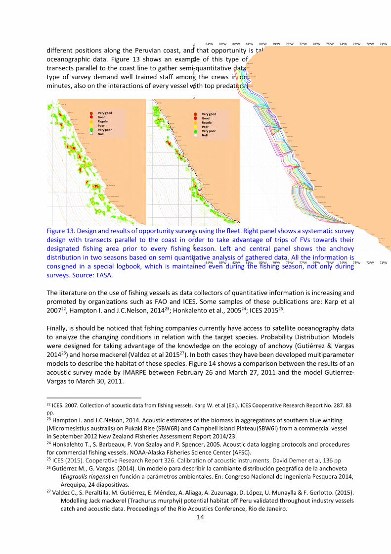
different positions along the Peruvian coast, and that opportunity is taken for collecting acoustic and oceanographic data. Figure 13 shows an example of this type of opportunity survey designed with transects parallel to the coast line to gather semi-quantitative data on the distribution of anchovy. This type of survey demand well trained staff among the crews in order to collect information every 15 minutes, also on the interactions of every vessel with top predators (sea birds and mammals).
Figure 13. Design and results of opportunity surveys using the fleet. Right panel shows a systematic survey design with transects parallel to the coast in order to take advantage of trips of FVs towards their designated fishing area prior to every fishing season. Left and central panel shows the anchovy distribution in two seasons based on semi quantitative analysis of gathered data. All the information is consigned in a special logbook, which is maintained even during the fishing season, not only during surveys. Source: TASA. The literature on the use of fishing vessels as data collectors of quantitative information is increasing and promoted by organizations such as FAO and ICES. Some samples of these publications are: Karp et al 200722, Hampton I. and J.C.Nelson, 201423; Honkalehto et al., 200524; ICES 201525. Finally, is should be noticed that fishing companies currently have access to satellite oceanography data to analyze the changing conditions in relation with the target species. Probability Distribution Models were designed for taking advantage of the knowledge on the ecology of anchovy (Gutiérrez & Vargas 201426) and horse mackerel (Valdez et al 201527). In both cases they have been developed multiparameter models to describe the habitat of these species. Figure 14 shows a comparison between the results of an acoustic survey made by IMARPE between February 26 and March 27, 2011 and the model Gutierrez-Vargas to March 30, 2011.
22 ICES. 2007. Collection of acoustic data from fishing vessels. Karp W. et al (Ed.). ICES Cooperative Research Report No. 287. 83 pp. 23 Hampton I. and J.C.Nelson, 2014. Acoustic estimates of the biomass in aggregations of southern blue whiting (Micromesistius australis) on Pukaki Rise (SBW6R) and Campbell Island Plateau(SBW6I) from a commercial vessel in September 2012 New Zealand Fisheries Assessment Report 2014/23. 24 Honkalehto T., S. Barbeaux, P. Von Szalay and P. Spencer, 2005. Acoustic data logging protocols and procedures for commercial fishing vessels. NOAA-Alaska Fisheries Science Center (AFSC). 25 ICES (2015). Cooperative Research Report 326. Calibration of acoustic instruments. David Demer et al, 136 pp 26 Gutiérrez M., G. Vargas. (2014). Un modelo para describir la cambiante distribución geográfica de la anchoveta
(Engraulis ringens) en función a parámetros ambientales. En: Congreso Nacional de Ingeniería Pesquera 2014, Arequipa, 24 diapositivas.
27 Valdez C., S. Peraltilla, M. Gutiérrez, E. Méndez, A. Aliaga, A. Zuzunaga, D. López, U. Munaylla & F. Gerlotto. (2015). Modelling Jack mackerel (Trachurus murphyi) potential habitat off Peru validated throughout industry vessels catch and acoustic data. Proceedings of the Rio Acoustics Conference, Rio de Janeiro.
19
ºS1
8ºS
17
ºS1
6ºS
15
ºS1
4ºS
13
ºS1
2ºS
11
ºS10
ºS9ºS
8ºS
7ºS
6ºS
5ºS
4ºS
3ºS
84ªW 83ªW 82ªW 81ªW 80ªW 79ªW 78ªW 77ªW 76ªW 75ªW 74ªW 73ªW 72ªW 71ªW 70ªW
84ªW 83ªW 82ªW 81ªW 80ªW 79ªW 78ªW 77ªW 76ªW 75ªW 74ªW 73ªW 72ªW 71ªW 70ªW
18
ªS1
7ªS
16
ªS1
5ªS
14
ªS1
3ªS
12
ªS1
1ªS
10
ªS9
ªS8ªS
7ªS
6ªS
5ªS
4ªS
Cabo Blanco
Talara
Paita
Pta. Gobernador
Pta. Falsa
Mórrope
Pimentel
Chérrepe
Chicama
Salaverry
Punta Chao
Chimbote
Casma
Punta Lobos
Huarmey
Punta Bermejo
Supe
Huacho
Chancay
Callao
Pucusana
Cerro Azul
Tambo de Mora
Pisco
Bahía Independencia
Punta Infiernillos
Punta Caballas
Lomas
San Juan
Chala
Atico
Ocoña
Quilca
Mollendo
Pta. El Carmen
Ilo
M. Sama
Palos
muy buena pescabuenaregularpocamuy poca pescanulo
Very good
Good
Regular
Poor
Very poor
Null
Very good
Good
Regular
Poor
Very poor
Null

15
Figure 14. Comparison between results of an acoustic assessment developed during 30 days (on the left) and the model of probability distribution for anchovy (on the right, according to Gutierrez-Vargas 2014) based on 7 parameters. The continuous use of FVs collectors of information can allow refine the models, which are useful for the management of the companies, as well as for scientific purposes and the management of the fishery. Source: IMARPE - TASA
5.2. The near field, blind areas and avoidance problems to acoustic assessment of biomass The "near field" is a phenomenon produced by magnetostriction of a number of elements composing a transducer. Every emission or transmission of sound (“ping”) creates a mechanic perturbation characterized by a number of beams produced around a main lobe which concentrates much of the intensity. Then the transmitted signal is chaotic in the area close to the transducer, and is the reason to remove it from acoustic analysis. Another reason to avoid this region is because the trigger of every ping is there and proportional to the used pulse length multiplied by sound speed (typically a pulse length duration is of 0.256 milliseconds, sound speed 1,500 m/s, then the length of the pulse is approximately 38 cm.) According to Simmonds & MacLennan (2005) the boundary between the near filed and "far-field" is solved with the following equation (where a is the radius of the transducer and λ is the wavelength of the emitted sound): CC = 2a2 / λ For a 120 kHz transducer this represents a distance of 1.6 m. However, because a precautionary approach in Peru is being used the double of that distance, typically 3.5 and up to 4 m. This area of 4 meters, added to the draft of the boat (in the case of FRV Olaya is 5 meters) generates 9 meters in which the echo sounder cannot detect fish, and therefore is formed a blind area for the assessment. Figure 15 schematically shows the problem of the blind zone near the surface. On the left side of figure 15 the fish is distributed below the limit between the near-field and far-field (represented by a red line), where it can be detected by the echo sounder. On the right side of figure 15 it can be seen that if fish move up to the surface will be undetectable. This effect can be partially and statistically compensated by using measured values located immediately below the boundary between near and far field.
Según IMARPE(26 de febrero a 27 marzo)
Según TASA(30 marzo)
Contundenciade pesca
Regular
Ralo
Muy ralo
negativo
According to IMARPEFebruary 26 to March 27
According to TASAMarch 30
Very good
Good
Regular
Poor
Very poor
Null

16
Figure 15. Schematics of the near field and blind area near the surface. Apperture or sensibility of used transducers typically is 7 degrees. Source: the authors. Another aspect that needs to be addressed as a priority is the avoidance, i.e., the evasion reactions of fish against the passage of a vessel, which adds uncertainty to acoustic assessments. Faced with this problem, there are two possible solutions, or both: 1) the placement of a transducer laterally oriented to measure the relative abundance of fish that are not accessible to the vertical echo-sounder (Figure 16); and 2) the use of a multibeam omnidirectional sonar which already is used aboard FVs (also available at FRV Olaya). In Peru there is a lack of experience on the quantitative use of sonars although tools for it (software) is however available. It is required therefore to develop knowledge and capacities on that regard. Following that idea courses and training workshops are necessary to generate knowledge on the use of the omnidirectional sonar technology. The Peruvian fishery is very important to the world, and therefore the investment in these improvements is widely justified.
Figure 16. The probability of detecting fish vertically with sound is low on certain occasions. The "near field" problem makes useless the first 4 to 5 m from the transducer. That, besides de draft of the ship, adds meters to the "blind area". Furthermore the noise radiated by the vessel increases the fish avoidance and reduce even more the possibilities of vertical detection vertical. This could be partly solved by using a transducer laterally oriented as shown in the figure. However, this use should be documented in the corresponding protocol of acoustic assessments. Source: the authors.
5.3. Use of the variogram as an indicator of the structure of clusters of fish In Peru the potential of geostatistics tools is not well exploited except for the calculation of gravity center of the distribution of fish. Inertia and global collocation index among others are not being used as
7°
Calado (3 a 6 m dependiendo del barco)
Campo cercano (1 a 3 m dependiendo de la frecuencia)
7°
17
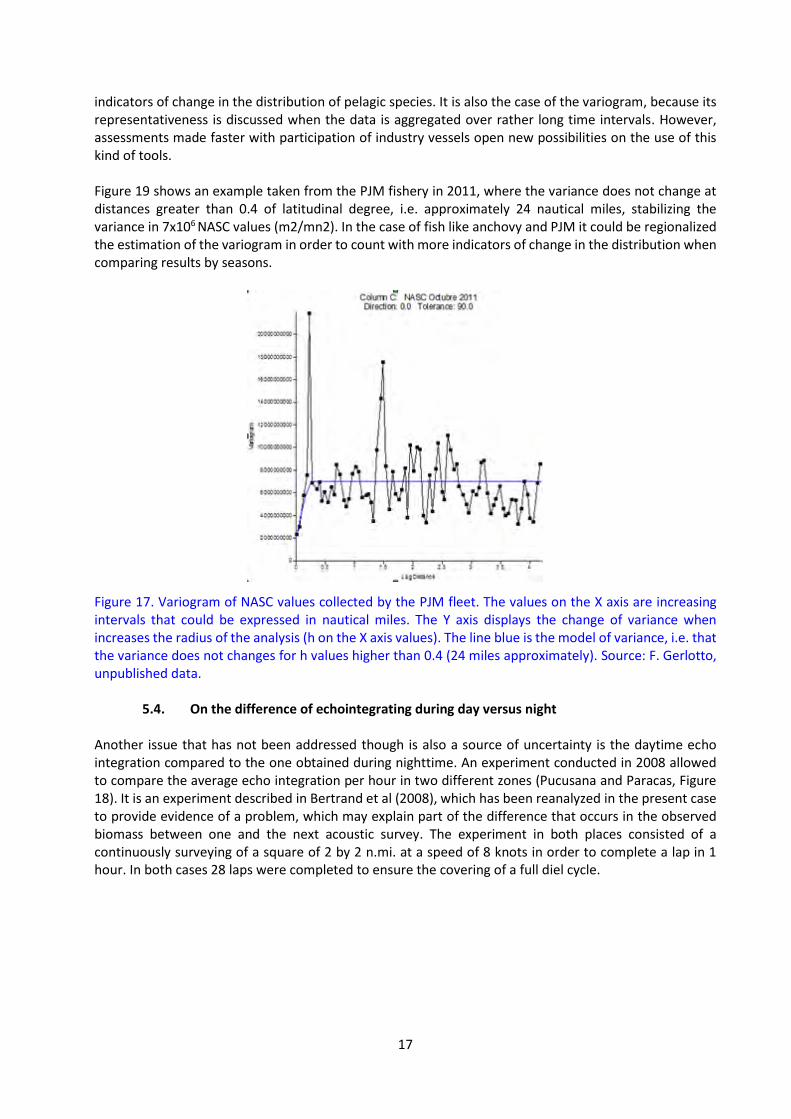
indicators of change in the distribution of pelagic species. It is also the case of the variogram, because its representativeness is discussed when the data is aggregated over rather long time intervals. However, assessments made faster with participation of industry vessels open new possibilities on the use of this kind of tools. Figure 19 shows an example taken from the PJM fishery in 2011, where the variance does not change at distances greater than 0.4 of latitudinal degree, i.e. approximately 24 nautical miles, stabilizing the variance in 7x10⁶ NASC values (m2/mn2). In the case of fish like anchovy and PJM it could be regionalized the estimation of the variogram in order to count with more indicators of change in the distribution when comparing results by seasons. Figure 17. Variogram of NASC values collected by the PJM fleet. The values on the X axis are increasing intervals that could be expressed in nautical miles. The Y axis displays the change of variance when increases the radius of the analysis (h on the X axis values). The line blue is the model of variance, i.e. that the variance does not changes for h values higher than 0.4 (24 miles approximately). Source: F. Gerlotto, unpublished data.
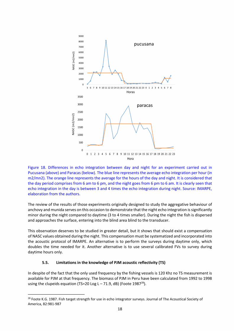
5.4. On the difference of echointegrating during day versus night Another issue that has not been addressed though is also a source of uncertainty is the daytime echo integration compared to the one obtained during nighttime. An experiment conducted in 2008 allowed to compare the average echo integration per hour in two different zones (Pucusana and Paracas, Figure 18). It is an experiment described in Bertrand et al (2008), which has been reanalyzed in the present case to provide evidence of a problem, which may explain part of the difference that occurs in the observed biomass between one and the next acoustic survey. The experiment in both places consisted of a continuously surveying of a square of 2 by 2 n.mi. at a speed of 8 knots in order to complete a lap in 1 hour. In both cases 28 laps were completed to ensure the covering of a full diel cycle.
18
Figure 18. Differences in echo integration between day and night for an experiment carried out in Pucusana (above) and Paracas (below). The blue line represents the average echo integration per hour (in m2/mn2). The orange line represents the average for the hours of the day and night. It is considered that the day period comprises from 6 am to 6 pm, and the night goes from 6 pm to 6 am. It is clearly seen that echo integration in the day is between 3 and 4 times the echo integration during night. Source: IMARPE, elaboration from the authors. The review of the results of those experiments originally designed to study the aggregative behaviour of anchovy and munida serves on this occasion to demonstrate that the night echo integration is significantly minor during the night compared to daytime (3 to 4 times smaller). During the night the fish is dispersed and approaches the surface, entering into the blind area blind to the transducer. This observation deserves to be studied in greater detail, but it shows that should exist a compensation of NASC values obtained during the night. This compensation must be systematized and incorporated into the acoustic protocol of IMARPE. An alternative is to perform the surveys during daytime only, which doubles the time needed for it. Another alternative is to use several calibrated FVs to survey during daytime hours only.
5.5. Limitations in the knowledge of PJM acoustic reflectivity (TS) In despite of the fact that the only used frequency by the fishing vessels is 120 Khz no TS measurement is available for PJM at that frequency. The biomass of PJM in Peru have been calculated from 1992 to 1998 using the clupeids equation (TS=20 Log L – 71.9, dB) (Foote 198728).
28 Foote K.G. 1987. Fish target strength for use in echo integrator surveys. Journal of The Acoustical Society of America, 82:981-987
0
1000
2000
3000
4000
5000
6000
7000
8000
9000
5 6 7 8 9 10 11 12 13 14 15 16 17 18 19 20 21 22 23 0 1 2 3 4 5 6 7 8
NA
SC (
m2
/mn
2)
Horas
0
500
1000
1500
2000
2500
3000
3500
0 1 2 3 4 5 6 7 8 9 10 11 12 13 14 15 16 17 18 19 20 21 22 23
NA
SC
(m
2/m
n2
)
Hora
pucusana
paracas

19
There is a measurement made in Peru in 1998 at 38 kHz (Gutierrez 200229), where the b20 intercept of the TS-Size regression was -68.15 dB. However the calculations of PJM biomass have been all made using the Lillo et al (199530) equation, where the b20 intercept is -68.91 dB. For Trachurus capensis in South Africa Barange et al (1996) found a b20 value of -66.8 dB. The most comprehensive study on TS of PJM to date was published by Peña & Foote (200831). In that study, the fish used for modelling were collected during in situ TS measurements of OJM off Chile during 2003 (Peña, 200832). As the range in mean lengths of the used three catches was so limited, only a single-parameter regression analysis was performed, namely TS = 20 log L +b20, where TS is the mean in situ TS and L the mean length in centimeters. The value of the coefficient and intercept b20 was -66 dB, a value different from the obtained by Peña & Foote, in which b20 varied between -74.9 and -72.1 dB. Some reasons were accounted to explain such a difference (using the -72.1 dB value would represent a biomass 2 times higher than previous estimations) and a conclusion was made on testing other technological approaches such as multifrequency. TS of the assessed species is of the greatest importance in acoustic assessments. Here we propose to perform experiments with live fish, both in situ and ex situ using submarine video cameras to gain knowledge on the tilt angle effect on TS.
6. Conclusions
Acoustic assessments carried out in Peru are under international standards. However there are limitations that do not allow to accurately measure the observed biomass of anchovy and other pelagic species.
Used acoustic protocols should be updated to incorporate the systematization of the calculation of the hidden biomass during fish stock assessments, specifically in the blind zone near the surface, the area near the bottom and in shallow areas. Also is must be studied and defined the method that should be employed to compensate the minor echo integration produced at night time.
The used protocols should permit to identify as appropriate the fishing vessels equipped and calibrated to participate in acoustic assessments. This participation not only allows to extend the commitment of the industry regarding the ecosystem, but represents a saving of time and financial resources to IMARPE. Also this use of fishing vessels allows to perform assessments in reduced time in comparison with conventional surveying. Furthermore this use reduces all the related biases inherent to acoustic methods (especially the bias due to vertical and horizontal migration).
In that sense, they have been tested the consistency among the acoustic measurements obtained by fishing vessels that deploy calibrated echo sounders with the measures obtained with scientific echo sounders of IMARPE. A Protocol for Calibration, Intercalibration and Removal of Noise and Interferences made by the UNFV in cooperation with SNP is effective and available to fishing companies and IMARPE.
29 Gutierrez M.(2002). Determinación de la Fuerza de Blanco de las principales especies del Mar Peruano. Universidad Nacional Federico Villareal. Tesis. 81 pp. 30 Lillo S, J Cordova, A. Paillaman.(1995). Target Strength measurements of hake and jack mackerel. ICES Journal of Marine Science, 53: 267-271. 31 Peña H., K.G. Foote. (2008). Modelling the target strength of Trachurus symmetricus murphyi based on high-resolution swimbladder morphometry using an MRI scanner. International Council for the Exploration of the Sea. Published by Oxford Journals 32 Peña, H. 2008. In situ target-strength measurements of Chilean jack mackerel (Trachurus symmetricus murphyi) collected with a scientific echo sounder installed on a fishing vessel. ICES Journal of Marine Science, 65: 594–604.

20
7. Recommendations
In line with recommendations made by FAO it must be strengthen the technical relationship among scientific entities and the industry in order to expand their research with support of universities.
To create a working group (WG) that specifically address the improvements for the next version of the acoustic Protocol of IMARPE, which must include methods to compensate the biomass that is hidden to the assessments in the blind and shallow areas. Also this WG should statistically analyze the way of compensating for the lower echo integration measured in night time.
IMARPE and the industry should also develop a strategy and method for continuously studying the fish avoidance, which is another factor of underestimation. The best way to do this is through the use of sonar technology. It is recommended to request support from MCM (South Africa) and relevant producers of technology (Simrad, Echoview Software Pty Ltd).
To strengthen the IMARPE cooperation with universities and local and international scientific bodies. That interaction will allow to enrich their research and improve the performance of the scientific staff. It is finally special to remember the important achievements made thanks to the cooperation of IMARPE and IRD (France).
8. References
Bertrand A., F. Gerlotto, S. Bertrand, M. Gutiérrez, L. Alza, A. Chipollini, E. Díaz, P. Espinoza, J. Ledesma, R.
Quesquén, S. Peraltilla, F. Chavez. (2008). Schooling behaviour and environmental forcing in relation to anchoveta distribution: An analysis across multiple spatial scales. Progress in Oceanography 79 (2008) 264–277
Bertrand, A., Ballon, M., and Chaigneau, A. (2010). Acoustic observation of living organisms reveals the upper limit of the oxygen minimum zone. PloS One 5, p. e10330
Bertrand, A., Grados, D., Colas, F., Bertrand, S., Capet, X., Chaigneau, A., Vargas, G., Mousseigne, A., and Fablet, R. (2014). Broad impacts of fine-scale dynamics on seascape structure from zooplankton to seabirds. Nature Communications 5.
Bertrand, S. (2005). Analyse comparée des dynamiques spatiales des poissons et des pêcheurs : mouvements et distributions dans la pêcherie d’anchois (Engraulis Ringens) du Pérou.
Demer, D.A., Berger, L., Bernasconi, M., Bethke, E., Boswell, K., Chu, D., Domokos, R., et al. 2015. Calibration of acoustic instruments. ICES Cooperative Research Report No. 326. 133pp. Foote K.G. 1987. Fish target strength for use in echo integrator surveys. Journal of The Acoustical Society of America, 82:981-987
Foote, K. G., Knudsen, H. P., Vestnes, G., MacLennan, D. N., and Simmonds, E. J. (1987). Calibration of acoustic instruments for fish density estimation: a practical guide. ICES Cooperative Research Report No. 144. 69 pp.
Foote, K.G. (1983).Maintaining precision calibrations with optimal copper spheres.Journal of theAcoustical Society of America. Foote, K.G. (1983).Maintaining precision calibrations with optimal copper spheres.Journal of theAcoustical Society of America.
Fréon, P., Cury, P., Shannon, L.J., and Roy, C. (2005). Sustainable exploitation of small pelagic fish stocks challenged by environmental and ecosystem changes : a review. Bulletin of Marine Science 76, 385–462
Gutierrez M.(2002). Determinación de la Fuerza de Blanco de las principales especies del Mar Peruano. Universidad Nacional Federico Villareal. Tesis. 81 pp.
Gutiérrez M., G. Vargas. (2014). Un modelo para describir la cambiante distribución geográfica de la anchoveta (Engraulis ringens) en función a parámetros ambientales. En: Congreso Nacional de Ingeniería Pesquera 2014, Arequipa, 24 diapositivas.
Hampton I. and J.C.Nelson, 2014. Acoustic estimates of the biomass in aggregations of southern blue whiting (Micromesistius australis) on Pukaki Rise (SBW6R) and Campbell Island Plateau(SBW6I) from a commercial vessel in September 2012 New Zealand Fisheries Assessment Report 2014/23.
21
Honkalehto T., S. Barbeaux, P. Von Szalay and P. Spencer, 2005. Acoustic data logging protocols and procedures for commercial fishing vessels. NOAA-Alaska Fisheries Science Center (AFSC).
ICES (2015). Cooperative Research Report 326. Calibration of acoustic instruments. David Demer et al, 136 pp
ICES. 2007. Collection of acoustic data from fishing vessels. Karp W. et al (Ed.). ICES Cooperative Research Report No. 287. 83 pp. Lillo S, J Cordova, A. Paillaman.(1995). Target Strength measurements of hake and jack mackerel. ICES Journal of Marine Science, 53: 267-271.
Mitson, R.B. (Ed.), 1995. Underwater Noise of Research Vessels: Review and Recommendations. ICES Coop. Res. Rep. No. 209, 61.
Peña H., K.G. Foote. (2008). Modelling the target strength of Trachurus symmetricus murphyi based on high-resolution swimbladder morphometry using an MRI scanner. International Council for the Exploration of the Sea. Published by Oxford Journals
Peña, H. 2008. In situ target-strength measurements of Chilean jack mackerel (Trachurus symmetricus murphyi) collected with a scientific echo sounder installed on a fishing vessel. ICES Journal of Marine Science, 65: 594–604.
Ryan T., R. Kloser. 2004. Quantification and correction of a systematic error in Simrad ES60 echo sounders. Technical Note, FAST ICES Working Group, Dansk, Poland. 9 pp. Ryan T., R. Kloser. 2004. Quantification and correction of a systematic error in Simrad ES60 echo sounders. Technical Note, FAST ICES Working Group, Dansk, Poland. 9 pp.
Simmonds EJ, MacLennan DN. Fisheries Acoustics: Theory and Practice, 2nd edn. London: Blackwell Science; 2005. 437 p.
Simmonds, E.J., Gutiérrez, M., Chipollini, A., Gerlotto, F., Woillez, M., and Bertrand, A. (2009). Optimizing the design of acoustic surveys of Peruvian anchoveta. ICES Journal of Marine Science 66.
Simrad. 2008. ER60 Scientific echo sounder software reference manual , Simrad Subsea A/S, Horten, Norway. 221 pp.
Valdez C., S. Peraltilla, M. Gutiérrez, E. Méndez, A. Aliaga, A. Zuzunaga, D. López, U. Munaylla & F. Gerlotto. (2015). Modelling Jack mackerel (Trachurus murphyi) potential habitat off Peru validated throughout industry vessels catch and acoustic data. Proceedings of the Rio Acoustics Conference, Rio de Janeiro.
Vargas G. (2013). Localization of fishing grounds for the Peruvian fishing fleet using acoustics and geoestatistical methods. Thesis. Universidad Nacional Federico Villarreal, 55 pp.