6. analysis - fun3d manual · 2020-05-22 · 6/5/2014 fun3d manual :: chapter 6: analysis /...
TRANSCRIPT

6/5/2014 FUN3D Manual :: Chapter 6: Analysis
http://fun3d.larc.nasa.gov/chapter-6.html 1/77
Current Release: 12.4-70371Site Last Updated: Wed Jun 04 16:41:01 -0400 2014
SITE CONTENTS
CHAPTERS
I. Introduction1. Background2. Capabilities3. Requirements4. Release History5. Request FUN3D
II. Installation1. Third-Party Libraries2. Compiling
III. Grid Generation1. 2D Grid Generation2. 3D Grid Generation
IV. Boundary Conditions1. Boundary Condition List2. Value Input Format (Version
11.0)V. Pre/Post Processing
1. Grid/Solution Processing withv11.0 and Higher
2. Sequential Grid Processing3. Parallel Grid Processing
VI. Analysis ←1. Flow Solver Namelist Input2. Running The Flow Solver3. Rotorcraft4. Hypersonics5. Time Accurate – Basics/Fixed
Geometry6. Time Accurate – Moving
Geometry7. Overset Grids8. Static Aeroelastic Coupling9. Ginput.faces Type Input
10. Flow Visualization OutputDirectly From Flow Solver
11. Individual Component ForceTracking
12. Static Grid Transforms13. Noninertial Reference Frame
VII. Adaptation and Error Estimation1. Capabilities2. Mesh Movement via Spring
Analogy3. Requirements and Configuring
to use refine4. Adjoint-Based Adaptation5. Gradient/Feature-Based
Adaptation6. Error Estimation
VIII. Design1. Getting Started2. Setting Up rubber.data3. Geometry Parameterizations4. The Adjoint Solver5. Running the Optimization6. Customization7. Forward-Mode Differentiation
IX. Appendix1. Publications2. Presentations and Other
Materials3. Development Team4. F95 Coding Standard5. Hypersonic Benchmarks
TRAINING WORKSHOPS
I. March 2010 Workshop1. Overview2. Agenda3. Images
II. April 2010 Workshop1. Overview2. Agenda and Training Materials3. Images
III. July 2010 Workshop1. Overview2. Agenda and Training Materials
IV. March 2014 Workshop1. Overview2. Agenda and Training Materials
V. Future Workshops
Previous (C5: Pre/Post Processing) | Up | Next (C7: Adaptation and Error Estimation)
6. ANALYSIS
6.1. FLOW SOLVER NAMELIST INPUT
Questions about any of the following can be emailed to FUN3D Support.
To run the FUN3D solver, you will need to pre-process your grid using the included Party utility.Once you have successfully run your grid through Party, running the flow solver is simply a matter ofsetting up the input namelist file, fun3d.nml, which is described in detail below.
Note that as of release 10.5.0, this namelist file replaces the old input deck, ginput.faces. If youhave an old ginput.faces file, there is a translator called ginput_translator in theutils/Namelist_new directory that reads ginput.faces and writes out a corresponding filefun3d.nml (as well as a more descriptive file fun3d.long.nml if preferred, which must be renamedto be fun3d.nml before using). If a ginput.faces file does not exist, then ginput_translator willcreate a fun3d.nml file with default values in it. IMPORTANT NOTE: as new namelists andparameters are added to the fun3d.nml file, these will generally not be output by the translatorprogram. In other words, ginput_translator gives only all defaults for namelist parametersassociated with the original ginput.faces deck, but it will not keep up with subsequently-addedparameters. As users get used to the new namelist method and ginput.faces fades into history, theneed for the translator program will go away.
In the new namelist input, the perfect gas and generic gas input parameters have been combined to agreater degree than was done in the old ginput.faces input deck. However, it should be noted thatthe earliest versions of this new namelist mostly do no more than mimic the ginput.faces filecapabilities. Thus, in many instances certain parameters work only for generic cases or only for ideal-gas cases. As time passes, it is hoped to merge the capabilities better, and remove many of theserestrictions and special cases. Thus, it is likely that changes may occur in fun3d.nml as it is workedand revised. The reason for having the input_version parameter in namelist &version_number (inthe file) is to help keep track of any significant changes that take place. It is also possible that thenaming convention and/or usage of fun3d.nml may change at some point in the future. Any suchchanges will be documented.
Please report any problems, inconsistencies, issues, etc. with the new fun3d.nml input to FUN3DSupport.
Documentation for the old ginput.faces can still be found in Ginput.faces Type Input Runningwith the old ginput.faces can be recovered by hardwiring the parameter namelist_ginput =.false. in routine io.f90. If you set this, then FUN3D will look for and read ginput.faces like itused to, instead of using the new fun3d.nml file.
A typical namelist file (with lots of comments) is shown here:
! This file contains namelists used for specifying inputs to ! FUN3D. For this version, the following namelists apply (if a ! namelist is not present, its variables take on their default ! values): ! version_number ! project ! governing_equations ! reference_physical_properties ! force_moment_integ_properties ! inviscid_flux_method ! turbulent_diffusion_models ! nonlinear_solver_parameters ! linear_solver_parameters ! code_run_control

6/5/2014 FUN3D Manual :: Chapter 6: Analysis
http://fun3d.larc.nasa.gov/chapter-6.html 2/77
1. Overview
TUTORIALS
I. Introduction1. See also
II. Flow Solver1. Inviscid flow solve2. Turbulent flow solve3. Merge VGRID mesh into mixed
elements and run solutionIII. Grid Motion
1. Overset Moving GridsIV. Design Optimization
1. Max L/D for steady flow2. Max L/D for steady flow at two
different Mach numbers3. Lift-constrained drag
minimization for DPW wing4. Max L/D over a pitching cycle for
a wing5. Max L/D for steady flow over a
wing-body-tail using SculptorV. Geometry Parameterization
1. MASSOUD2. Bandaids
APPLICATIONS
1. Updated scaling study on ORNL CrayXK7 system
2. Forward and adjoint solutions for windturbine
3. Forward and adjoint solutions foraeroelastic F-15
4. Simulation of biologically-inspiredflapping wing
5. Notional unducted engine withcounter-rotating blades
6. More applications posters7. Animation of Landing Gear
Simulations8. Computational Schlierens for
Supersonic Retro-Propulsion9. Time-dependent discrete adjoint
solution for UH60 helicopter in forwardflight
10. Fuselage effects for UH60 helicopter11. Mesh adaptation for RANS simulation
of supersonic business jet12. More applications posters13. Horizontal axis wind turbine14. BMI's Mike Henderson describes the
role of CFD and HPC in tractor-traileranalysis and design
15. Computational Schlieren for UnsteadySimulation of Launch Abort System
16. Computational vs ExperimentalSchlieren for Supersonic Retro-Propulsion
17. More Smart Truck Simulations at BMICorporation
18. More recent applications at AMRDEC19. Hypersonic Winnebago Simulation20. Flight Trajectories for Various Rocket
Geometries21. Supersonic Retro-Propulsion22. Smart Truck Simulations at BMI
Corporation23. Ongoing Improvements in
Computational Performance24. Long-duration Landing Gear
Simulations25. Design of Tiltrotor Configuration26. Design of F-15 with Simulated
Aeroelastic Effects27. FUN3D and LAURA v5 STS-2 heating
comparisons28. Recent applications at AMRDEC29. DES ground wind simulation on ARES
configuration30. Modified F-15 with Propulsion Effects31. Mars Science Laboratory32. Propulsion-Related Test Cases33. Recent Applications at BMI
Corporation34. Applications Posters35. Mars Phoenix Lander36. CLV Analysis37. Robin Helicopter38. Dynamic Overset Grid Demonstration
Using A Simple Rotor/Fuselage Model39. Hypersonic Tethered Ballute
Simulation40. Time-Dependent Oscillating Flap
Demonstration41. Adjoint-Based Adaptation Applied to
AIAA DPW II Wing-Body42. Adjoint-Based Adaptation Applied to
High-Lift Airfoil43. Trapezoidal High-Lift Wing44. Adjoint-Based Adaptation Applied to
Supersonic Double-Airfoil45. Partial-Span Flap
! special_parameters ! component_parameters !
&version_number input_version = 2.2 ! version number of namelist file ! (ginput.faces: N/A) ! DEFAULT varies namelist_verbosity = "off" ! current options: on, off, suppress_all ! (ginput.faces: N/A) ! DEFAULT=off /
&project project_rootname = "default_project" ! DEFAULT=default_project ! (ginput.faces: PROJECT_NAME) case_title = "fun3d_case_name" ! DEFAULT=fun3d_case_name ! (ginput.faces: CASE TITLE) part_pathname = " " ! (ginput.faces: N/A) ! DEFAULT=" " (blank) /
&governing_equations eqn_type = "cal_perf_compress" ! current options: cal_perf_compress, ! cal_perf_incompress, generic ! (ginput.faces: INCOMP) ! DEFAULT=cal_perf_compress prandtlnumber_molecular = 0.72 ! (ginput.faces: PRANDTL) ! currently does nothing for generic path ! DEFAULT=0.72 artificial_compress = 15.0 ! artificial compressibility factor, only ! used when solver = cal_perf_incompress ! (ginput.faces: XMACH when INCOMP=1) ! DEFAULT=15.0 viscous_terms = "turbulent" ! current options: inviscid, laminar, ! turbulent (ginput.faces: IVISC) ! DEFAULT=turbulent chemical_kinetics = "finite-rate" ! current options: frozen, finite-rate ! (ginput.faces: CHEM_FLAG) ! does nothing for cal_perf paths ! DEFAULT=finite-rate thermal_energy_model = "non-equilib" ! current options: frozen, non-equilib ! (ginput.faces: THERM_FLAG) ! does nothing for cal_perf paths ! DEFAULT=non-equilib /
&reference_physical_properties gridlength_conversion = 1.0 ! sets L_REF for generic generic gas only ! DEFAULT=1.0 ! !------------------------------------------------------------- ! User must choose either NONDIMENSIONAL or DIMENSIONAL input: ! (one set is read and one is ignored depending on ! dim_input_type), Note, however, that temperature is always ! input as a dimensional number !------------------------------------------------------------- dim_input_type = "nondimensional" ! options: nondimensional, dimensional-SI ! (ginput.faces: N/A) ! DEFAULT=nondimensional temperature_units = "Kelvin" ! options: Kelvin, Rankine ! (ginput.faces: N/A) ! DEFAULT=Kelvin !------------------------------------------------------------- ! NONDIMENSIONAL INPUT: ! (generic : do not use) ! (cal_perf_compress : specify mach_number, ! reynolds_number) ! (cal_perf_incompress: specify reynolds_number only) !------------------------------------------------------------- mach_number = 0.2

6/5/2014 FUN3D Manual :: Chapter 6: Analysis
http://fun3d.larc.nasa.gov/chapter-6.html 3/77
46. Mach 24 Temperature-BasedAdaptation of Space ShuttleConfiguration in ChemicalNonequilibrium
47. Line Construction for Line-ImplicitRelaxation
48. Biologically-Inspired Morphing Aircraft49. Mars Flyer50. Support for QFF Tunnel Experiment51. Combined FUN3D/CFL3D F-1852. Adjoint-Based Adaptation for 3D Sonic
Boom53. Unsteady Space Shuttle Cable Tray
Analysis54. Adjoint-Based Design of Indy Car Wing55. 3D Domain Decomposition56. Mesh Movement Strategies57. High-Lift Computations vs Experiment58. Various 2D Adjoint-Based Airfoil
Designs
SOURCE CODE ACTIVITY
Subversion Commits
! (ginput.faces: XMACH) ! only used if ! dim_input_type=nondimensional ! currently does nothing for generic path ! DEFAULT=0.2 reynolds_number = 1000000.0 ! based on reference length of 1 grid_unit ! (ginput.faces: RE) ! only used if ! dim_input_type=nondimensional ! currently does nothing for generic path ! DEFAULT=1.e6 !------------------------------------------------------------- ! DIMENSIONAL INPUT: ! (generic : specify velocity and density) ! (cal_perf_compress : do not use) ! (cal_perf_incompress: do not use) !------------------------------------------------------------- velocity = 30.0 ! in m/s (ginput.faces: V_INF for generic) ! only used if ! dim_input_type=dimensional-SI ! currently does nothing for cal_perf paths ! DEFAULT=30.0 density = 0.1 ! in kg/m3 ! (ginput.faces: RHO_INF for generic) ! only used if ! dim_input_type=dimensional-SI ! currently does nothing for cal_perf paths ! DEFAULT=0.1 !------------------------------------------------------------- ! temperature = 273.0 ! in temperature_units ! (ginput.faces: TREF in Rankine for ! cal_perf paths, T_INF in Kelvin for ! generic) ! DEFAULT=273.0 temperature_walldefault = 0.0 ! in temperature_units; ! must be specified for generic ! (ginput.faces: T_WALL for generic); ! currently does nothing for cal_perf paths ! DEFAULT=0.0 angle_of_attack = 0.0 ! in degrees (ginput.faces: ALPHA) ! DEFAULT=0.0 angle_of_yaw = 0.0 ! in degrees (ginput.faces: YAW) ! DEFAULT=0.0 /
&force_moment_integ_properties area_reference = 1.0 ! area used to nondimensionalize forces and ! moments, in scaled_grid_units2 ! (ginput.faces: SREF) ! DEFAULT=1.0 x_moment_length = 1.0 ! length (in x-direction) used to nondimensionalize moments ! about y, in scaled_grid_units ! (ginput.faces: CREF) ! DEFAULT=1.0 y_moment_length = 1.0 ! length (in y-direction) used to nondimensionalize moments ! about x and about z, in scaled_grid_units ! (ginput.faces: BREF) ! DEFAULT=1.0 x_moment_center = 0.0 ! in scaled_grid_units (ginput.faces: XMC) ! DEFAULT=0.0 y_moment_center = 0.0 ! in scaled_grid_units (ginput.faces: YMC) ! DEFAULT=0.0 z_moment_center = 0.0 ! in scaled_grid_units (ginput.faces: ZMC) ! DEFAULT=0.0 /
&inviscid_flux_method flux_limiter = "none" ! current options: none, barth, venkat, ! minmod, vanleer, vanalbada, smooth, ! hminmod, hvanleer, hvanalbada, hsmooth

6/5/2014 FUN3D Manual :: Chapter 6: Analysis
http://fun3d.larc.nasa.gov/chapter-6.html 4/77
! (ginput.faces: IFLIM) ! DEFAULT=none first_order_iterations = 0 ! number of iterations or sub-iterations ! run 1st order (ginput.faces: NITFO) ! DEFAULT=0 flux_construction = "roe" ! current options: vanleer, roe, hllc, ! aufs, central_diss, ldfss, dldfss, stvd, ! stvd_modified; only roe allowed for ! cal_perf_incompress (ginput.faces: IHANE) ! DEFAULT=roe rhs_u_eigenvalue_coef = 0.0 ! (ginput.faces: EIG0 for generic) ! currently does nothing for cal_perf paths ! DEFAULT=0.0 lhs_u_eigenvalue_coef = 0.0 ! (ginput.faces: EIG0_IMP for generic) ! currently does nothing for cal_perf paths ! DEFAULT=0.0 /
&turbulent_diffusion_models turb_model = "sa" ! current options: sa, des, sst, ! sst-v, abid-ke, hrles, gamma-ret-sst ! (ginput.faces: IVISC or TURB_MODEL_TYPE) ! DEFAULT=sa turb_intensity = 2.0E-003 ! Tu = sqrt(2k/(3uinf2)), k=turb K.E. ! (ginput.faces: TURB_INT_INF for generic) ! currently does nothing for cal_perf paths ! DEFAULT=0.002 turb_viscosity_ratio = 0.210438 ! mu_t/mu_molecular ! (ginput.faces: TURB_VIS_RATIO_INF ! for generic) ! currently does nothing for cal_perf paths ! DEFAULT=0.210438 re_stress_model = "linear" ! current options: linear or nonlinear ! (ginput.faces: REYNOLDS_STRESS_MODEL for ! generic) ! currently does nothing for cal_perf paths ! DEFAULT=linear turb_compress_model = "off" ! current options: on, off ! (ginput.faces: TURB_COMP_MODEL for ! generic) ! currently does nothing for cal_perf paths ! DEFAULT=off turb_conductivity_model = "off" ! current options: on, off ! (ginput.faces: TURB_COND_MODEL for ! generic) ! currently does nothing for cal_perf paths ! DEFAULT=off prandtlnumber_turbulent = 0.9 ! (ginput.faces: PRANDTL_TURB for generic) ! currently does nothing for cal_perf paths ! DEFAULT=0.9 schmidtnumber_turbulent = 1.0 ! not used by cal_perf paths ! (ginput.faces: SCHMIDT_TURB for generic) ! currently does nothing for cal_perf paths ! DEFAULT=1.0 / !------------------------------------------------------------- ! ADDITIONAL INPUT FOR SPALART AND DDES TURBULENCE MODEL !------------------------------------------------------------- &spalart turbinf = 3.0, ! free stream value for spalart model variable ! (DEFAULT changed from 1.341946 to 3.0 as of ! version 12.3) ddes = .true., ! used for activating delayed DES (DDES) model ! (DEFAULT=.false.) ddes_mod1 = .true., ! used for modification of DDES model ! (Ref. AIAA Paper 2010-4001) ! (DEFAULT=.false.) sarc = .true., ! used to invoke SARC model ! (Ref. AIAA Journal Vol. 38, No. 5, 2000,
6/5/2014 FUN3D Manual :: Chapter 6: Analysis
http://fun3d.larc.nasa.gov/chapter-6.html 5/77
! pp. 784-792.) ! (DEFAULT=.false.) sarc_cr3 = 1.0, ! constant associated with SARC model ! (DEFAULT=0.6)/ !------------------------------------------------------------- ! ADDITIONAL INPUT FOR GAMMA-RET-SST TURBULENCE MODEL !------------------------------------------------------------- &gammaretsst set_k_inf_w_turb_intsty_percnt = 0.2 ! if used, overrides the default k_inf by ! using input turb intensity (percent) set_w_inf_w_eddyviscosity = 1.0 ! if used, overrides the default w_inf by ! using input eddy viscosity (nondim) transition_4eqn_on = .true., ! if .false., turns off transition part of model ! (DEFAULT=.true.)/
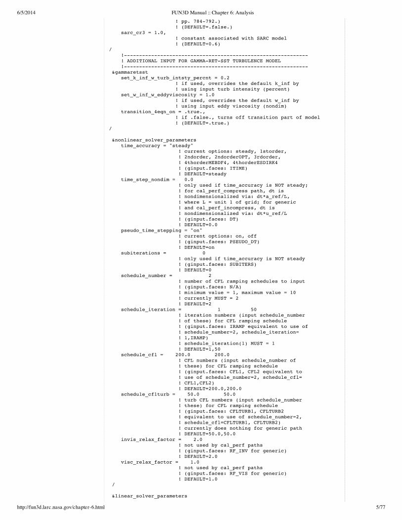
&nonlinear_solver_parameters time_accuracy = "steady" ! current options: steady, 1storder, ! 2ndorder, 2ndorderOPT, 3rdorder, ! 4thorderMEBDF4, 4thorderESDIRK4 ! (ginput.faces: ITIME) ! DEFAULT=steady time_step_nondim = 0.0 ! only used if time_accuracy is NOT steady; ! for cal_perf_compress path, dt is ! nondimensionalized via: dt*a_ref/L, ! where L = unit 1 of grid; for generic ! and cal_perf_incompress, dt is ! nondimensionalized via: dt*u_ref/L ! (ginput.faces: DT) ! DEFAULT=0.0 pseudo_time_stepping = "on" ! current options: on, off ! (ginput.faces: PSEUDO_DT) ! DEFAULT=on subiterations = 0 ! only used if time_accuracy is NOT steady ! (ginput.faces: SUBITERS) ! DEFAULT=0 schedule_number = 2 ! number of CFL ramping schedules to input ! (ginput.faces: N/A) ! minimum value = 1, maximum value = 10 ! currently MUST = 2 ! DEFAULT=2 schedule_iteration = 1 50 ! iteration numbers (input schedule_number ! of these) for CFL ramping schedule ! (ginput.faces: IRAMP equivalent to use of ! schedule_number=2, schedule_iteration= ! 1,IRAMP) ! schedule_iteration(1) MUST = 1 ! DEFAULT=1,50 schedule_cfl = 200.0 200.0 ! CFL numbers (input schedule_number of ! these) for CFL ramping schedule ! (ginput.faces: CFL1, CFL2 equivalent to ! use of schedule_number=2, schedule_cfl= ! CFL1,CFL2) ! DEFAULT=200.0,200.0 schedule_cflturb = 50.0 50.0 ! turb CFL numbers (input schedule_number ! these) for CFL ramping schedule ! (ginput.faces: CFLTURB1, CFLTURB2 ! equivalent to use of schedule_number=2, ! schedule_cfl=CFLTURB1, CFLTURB2) ! currently does nothing for generic path ! DEFAULT=50.0,50.0 invis_relax_factor = 2.0 ! not used by cal_perf paths ! (ginput.faces: RF_INV for generic) ! DEFAULT=2.0 visc_relax_factor = 1.0 ! not used by cal_perf paths ! (ginput.faces: RF_VIS for generic) ! DEFAULT=1.0 /
&linear_solver_parameters

6/5/2014 FUN3D Manual :: Chapter 6: Analysis
http://fun3d.larc.nasa.gov/chapter-6.html 6/77
meanflow_sweeps = 15 ! number of Gauss-Seidel sub-iterations for ! the linear problem at each time step ! (ginput.faces: NSWEEP) ! DEFAULT=15 turbulence_sweeps = 10 ! same, for turbulence; not used by generic ! path (ginput.faces: NCYCT) ! DEFAULT=10 line_implicit = "off" ! current options: on, off ! (ginput.faces: NSWEEP negative) ! DEFAULT=off /
&code_run_control steps = 500 ! number of time steps or multigrid cycles ! to run the code (ginput.faces: NCYC) ! DEFAULT=500 stopping_tolerance = 1.0E-015 ! absolute value of the RMS residual at ! which the solver will terminate early ! (ginput.faces: RMSTOL) ! DEFAULT=1.e-15 restart_write_freq = 250 ! frequency of restart write based on time ! steps or multigrid cycles ! (ginput.faces: ITERWRT) ! DEFAULT=250 restart_read = "on" ! current options: off, on, ! on_nohistorykept ! (ginput.faces: IREST) ! DEFAULT=on jacobian_eval_freq = 10 ! frequency of jacobian evaluation based on ! time steps or multigrid cycles ! (ginput.faces: JUPDATE) ! DEFAULT=10 /
&special_parameters large_angle_fix = "off" ! fix to neglect viscous fluxes in cells ! containing angles equal to 178 degrees or ! more; current options: on, off ! (ginput.faces: IVGRD) ! DEFAULT=off /
&flow_initialization number_of_volumes = 0 ! number of initialization volumes ! DEFAULT=0 type_of_volume(n)='none' ! volume definition index ! Current options: ! 'box, 'sphere', 'cylinder', 'cone' ! DEFAULT='none' pmin(1:3,n) = 0.0, 0.0, 0.0 ! coordinates of lower corner of box (n) ! DEFAULT= (0.0,0.0,0.0) pmax(1:3,n) = 0.0, 0.0, 0.0 ! coordinates of upper corner of box (n) ! DEFAULT= (0.0,0.0,0.0) center(1:3,n)= 0.0, 0.0, 0.0 ! coordinates of center of sphere (n) ! DEFAULT= (0.0,0.0,0.0) radius(n)=0.0 ! radius of sphere (n) ! DEFAULT= (0.0,0.0,0.0) point1(1:3,n) = 0.0, 0.0, 0.0 ! center of endpoint 1 of cylinder (n) ! DEFAULT= (0.0,0.0,0.0) point2(1:3,n) = 0.0, 0.0, 0.0 ! center of endpoint 2 of cylinder (n) ! DEFAULT= (0.0,0.0,0.0) radius(n) = 0.50 ! radius of cylinder (n) ! DEFAULT=0.0 point1(1:3,n) = 0.0, 0.0, 0.0 ! center of endpoint 1 of cone (n) ! DEFAULT= (0.0,0.0,0.0) point2(1:3,n) = 1.0, 0.0, 0.0

6/5/2014 FUN3D Manual :: Chapter 6: Analysis
http://fun3d.larc.nasa.gov/chapter-6.html 7/77
The comments given above describe the default for each parameter, and also give the correspondingentry from the old ginput.faces file. The comments in the file are not necessary. With this type ofinput file, leaving out or misspelling any namelist (the category parameter defined with an ampersand“&” preceding its name) will result in default values being used for all of the parameters within thatnamelist. For example, if the namelist name linear_solver_parameters were to be misspelled aslinear_solver_parameter (missing “s”), then all parameters within that namelist that you thinkyou are specifying would be ignored, and they would assume their default values. This is one goodreason to always leave namelist_verbosity = on, so the top of the screen output has a record notonly of what you input, but also what the code is using as well. Leaving out any parameter within anamelist results in the default value for that parameter being used. Misspelling or misusing anyparticular parameter will typically cause FUN3D to issue an error and stop.
Note that the above namelist file contains many input variables, but in general it is not necessary tolist them all. One can instead rely on the fact that most of the defaults are often desired, and onlythose variables that are different from the defaults need to be given. The following might be anexample of a typical namelist file for a calorically-perfect FUN3D run:
&version_number input_version = 2.2 / &project project_rootname = "my_project" / &reference_physical_properties mach_number = 0.84 reynolds_number = 6200000.0 temperature = 252.5 angle_of_attack = 13.7 / &force_moment_integ_properties area_reference = 500.2 x_moment_length = 16.444 y_moment_length = 2.2 x_moment_center = 0.25 / &inviscid_flux_method
! center of endpoint 1 of cone (n) ! DEFAULT= (0.0,0.0,0.0) radius1(n) = 0.10 ! radius of endpoint 1 of cone (n) ! DEFAULT=0.0 radius2(n) = 1.00 ! radius of endpoint 2 of cone (n) ! DEFAULT=0.0 rho(n) = 1.0 ! Density (n) ! DEFAULT=1.0 c(n) = 0.9 ! speed of sound (n) ! DEFAULT=1.0 u(n) = 0.4 ! u veloicty (n) ! DEFAULT=0.0 v(n) = 0.0 ! v velocity (n) ! DEFAULT=0.0 w(n) = 0.0 ! w velocity (n) ! DEFAULT=0.0/
&component_parameters number_of_components = 1 ! number of individual components to be tracked ! DEFAULT=0 component_count(n) = 3 ! number of boundaries to be included in each component force track ! DEFAULT=0 component_list(n) = '2,3,9' ! string list of boundary numbers for component_count(n) ! DEFAULT='' component_name(n) = 'body' ! name used in file header of component force tracking ! DEFAULT='' allow_flow_through_forces = .true. ! allows for nozzle and inlet boundaries to be included in force tracking ! DEFAULT = .false. /

6/5/2014 FUN3D Manual :: Chapter 6: Analysis
http://fun3d.larc.nasa.gov/chapter-6.html 8/77
flux_limiter = "smooth" / &turbulent_diffusion_models turb_model = "sst-v" / &nonlinear_solver_parameters schedule_iteration = 1 150 schedule_cfl = 25.0 200.0 schedule_cflturb = 10.0 50.0 / &code_run_control steps = 2000 restart_read = "off" / &component_parameters number_of_components = 1 component_count(1) = 2 component_list(1) = '1, 5' component_name(1) = 'InletCowl' allow_flow_through_forces = .true. /
Each of the namelists is described below. The defaults for each parameter can be found in the firstsample file above.
NAMELIST &VERSION_NUMBER
input_version The version number of the namelist file.namelist_verbosityDetermines how namelist information from fun3d.nml is written to the
screen output. When on, the file fun3d.nml is echoed to the screen outputalong with a list of all namelist parameters (including defaults). Additionalinformation and warnings (if necessary) are also given. This setting (on) isthe recommended option, because the user can check to see all of theparameters being used by the code, whether explicitly being specified in thenamelist file or implicitly being used by default. When off, only the inputfile fun3d.nml is echoed. When suppress_all, all writing of fun3d.nmlinformation to screen output is suppressed. Quotes are needed around thecharacter string.
NAMELIST &PROJECT
project_rootnameThe project name for the grid. For example, all grid part files and solution fileshave this rootname as part of their filename. Quotes are needed around thecharacter string.
case_title User-defined title for the case. Quotes are needed around the character string.part_pathname Either absolute path or relative path from the current working directory to the
location of the grid (part) files. Quotes are needed around the character string.
NAMELIST &GOVERNING_EQUATIONS
eqn_type Equation type being solved, for example cal_perf_compress forcalorically perfect compressible, cal_perf_incompress forcalorically perfect incompressible, generic for generic gas. Quotesare needed around the character string.
prandtlnumber_molecularMolecular Prandtl number.artificial_compress Artificial compressibility factor (beta), only used when eqn_type =
cal_perf_incompress.viscous_terms Describes viscous term usage, for example inviscid for no viscous
term (Euler), laminar for Navier-Stokes with no turbulence model,turbulent for Navier-Stokes with turbulence model. Quotes areneeded around the character string.
chemical_kinetics Describes the chemical kinetics, only used when eqn_type =generic, for example frozen for chemically frozen flow, finite-rate for finite-rate chemically-reacting flow. Quotes are neededaround the character string.
thermal_energy_model Describes the thermal energy model, only used when eqn_type =generic, for example frozen for frozen thermal energy treatment,non-equilib for non-equilibrium thermal energy. Quotes are neededaround the character string.

6/5/2014 FUN3D Manual :: Chapter 6: Analysis
http://fun3d.larc.nasa.gov/chapter-6.html 9/77
NAMELIST &REFERENCE_PHYSICAL_PROPERTIES
gridlength_conversion Conversion factor to scale the grid by. (generic gas only)dim_input_type Type of input, for example nondimensional or dimensional-SI.
The user’s choice here determines whether Mach number andReynolds number are input (for nondimensional), or dimensionalvelocity and density are input (for dimensional). Note, however, thattemperature is always input as a dimensional quantity. Quotes areneeded around the character string.
temperature_units Units for temperature, for example Kelvin or Rankine. Quotes areneeded around the character string.
mach_number Reference Mach number, velocity/speed-of-sound. Only used ifdim_input_type = nondimensional.
reynolds_number Reference Reynolds number, per unit 1 of the grid. For example, Ifyour Reynolds number is based on the MAC(Mean AerodynamicChord), and the grid is constructed so that the MAC is one, then theappropriate value for this is the full freestream Reynolds number. If thegrid is constructed so that the MAC is in inches, then this must be setto the Reynolds number divided by the MAC in inches. Only used ifdim_input_type = nondimensional.
velocity Reference velocity, in m/s, only used if dim_input_type =dimensional-SI.
density Reference density, in kg/m3^, only used if dim_input_type =
dimensional-SI.
temperature Reference temperature, in units of temperature_units.temperature_walldefaultWall temperature, currently only used for eqn_type = generic.
angle_of_attack Freestream angle of attack in degrees.angle_of_yaw Freestream angle of yaw (side-slip) in degrees.
NAMELIST &FORCE_MOMENT_INTEG_PROPERTIES
area_referenceReference area used for non-dimensionalization of forces and moments, inscaled_grid_units2.
x_moment_lengthReference length in x-direction, used to nondimensionalize moments about y, inscaled_grid_units.
y_moment_lengthReference length in y-direction, used to nondimensionalize moments about x andz, in scaled_grid_units.
x_moment_centerX-coordinate location of moment center, in scaled_grid_units.y_moment_centerY-coordinate location of moment center, in scaled_grid_units.
z_moment_centerZ-coordinate location of moment center, in scaled_grid_units.
NAMELIST &INVISCID_FLUX_METHOD
flux_limiter Flux limiter used, for example none for no limiter, barth for Barthlimiter, venkat for Venkatakrishnan limiter, minmod for min-modlimiter, vanleer for van Leer limiter, vanalbada for van Albadalimiter, smooth for smooth limiter, hminmod for hypersonic-minmodlimiter, hvanleer for hypersonic-van Leer limiter, hvanalbada forhypersonic-van Albada limiter, hsmooth for hypersonic-smooth limiter,and hvenkat for hypersonic-Vankatakrishnan limiter, For hypersonicflows computed using the calorically perfect gas path the hvanleer orhvanalbada flux limiters are recommended. Please note that use of theh-series of flux limiters automatically turns on a heuristic pressure basedlimiter that is used to augment the selected flux limiter. When using amixed element grid (where the near wall grid is made up of either hexesor prisms) the wall heat transfer and skin friction can be improved byselecting the hminmod, hvanleer, hvanalbada, hsmooth, or hvnekatlimiters and invoking the command line option --limit_near_walls_less. This option causes these flux limiter to beautomatically “turned off” as the grid approaches the wall. However useof this option on tetrahedral grids near the wall can make the wall heattransfer and skin friction worse. Use of this option may cause a decreasein robustness so use it with caution. When using the barth, venkat,hminmod, hvanleer, hvanalbada, hsmooth, or hvnekat limiter, the
6/5/2014 FUN3D Manual :: Chapter 6: Analysis
http://fun3d.larc.nasa.gov/chapter-6.html 10/77
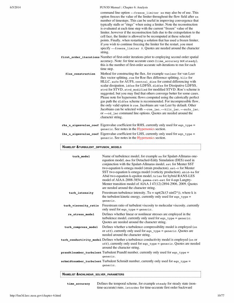
command line option --freeze_limiter xx may also be of use. Thisoption freezes the value of the limiter throughout the flow field after xxnumber of timesteps. This can be useful in improving convergence thattypically stalls or “rings” when using a limiter. Note the reconstructionis evaluated at each time step with the current “frozen” value of thelimiter, however if the reconstruction fails due to the extrapolation to thecell face, the limiter is allowed to be recomputed at these selectedpoints. Finally, when restarting a solution that has used a frozen limiter,if you wish to continue freezing the limiter for the restart, you mustspecify --freeze_limiter 0. Quotes are needed around the characterstring.
first_order_iterationsNumber of first-order iterations prior to employing second order spatialaccuracy. Note: for time accurate cases (time_accuracy not steady),this is the number of first-order accurate sub-iterations to run for eachtime step.
flux_construction Method for constructing the flux, for example vanleer for van Leerflux vector splitting, roe for Roe flux difference splitting, hllc forHLLC, aufs for AUFS, central_diss for central differencing withscalar dissipation, ldfss for LDFSS, dldfss for Dissipative LDFSS,stvd for STVD, stvd_modified for modified STVD. Roe’s scheme issuggested, but you may find that others converge better for some cases.Please note for hypersonic flows computed using the calorically perfectgas path the dldfss scheme is recommended. For incompressible flow,the only valid option is roe. Jacobians are van Leer by default. OtherJacobians can be selected with --roe_jac, --hllc_jac, --aufs_jac,or --cd_jac command line options. Quotes are needed around thecharacter string.
rhs_u_eigenvalue_coef Eigenvalue coefficient for RHS, currently only used for eqn_type =generic. See notes in the Hypersonics section.
lhs_u_eigenvalue_coef Eigenvalue coefficient for LHS, currently only used for eqn_type =generic. See notes in the Hypersonics section.
NAMELIST &TURBULENT_DIFFUSION_MODELS
turb_model Name of turbulence model, for example sa for Spalart-Allmaras one-equation model, des for Detached-Eddy Simulation (DES) used inconjunction with the Spalart-Allmaras model, sst for Menter SSTtwo-equation k-omega model (strain producton), sst-v for MenterSST two-equation k-omega model (vorticity production), abid-ke forAbid two-equation k-epsilon model, hrles for hybrid RANS-LESmodel of AIAA-2008-3854, gamma-ret-sst for 4-eqn Langtry-Menter transition model of AIAA J 47(12):2894-2906, 2009. Quotesare needed around the character string.
turb_intensity Freestream turbulence intensity, Tu = sqrt(2k/(3 uinf2^)), where k isthe turbulent kinetic energy, currently only used for eqn_type =generic.
turb_viscosity_ratio Freestream ratio of turbulent viscosity to molecular viscosity, currentlyonly used for eqn_type = generic.
re_stress_model Defines whether linear or nonlinear stresses are employed in theturbulence model, currently only used for eqn_type = generic.Quotes are needed around the character string.
turb_compress_model Defines whether a turbulence compressibility model is employed (onor off), currently only used for eqn_type = generic. Quotes areneeded around the character string.
turb_conductivity_modelDefines whether a turbulence conductivity model is employed (on oroff), currently only used for eqn_type = generic. Quotes are neededaround the character string.
prandtlnumber_turbulentTurbulent Prandtl number, currently only used for eqn_type =generic.
schmidtnumber_turbulentTurbulent Schmidt number, currently only used for eqn_type =generic.
NAMELIST &NONLINEAR_SOLVER_PARAMETERS
time_accuracy Defines the temporal scheme, for example steady for steady state (non-time-accurate) runs, 1storder for time-accurate first order backward
6/5/2014 FUN3D Manual :: Chapter 6: Analysis
http://fun3d.larc.nasa.gov/chapter-6.html 11/77
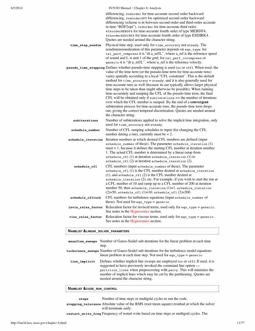
differencing, 2ndorder for time-accurate second order backwarddifferencing, 2ndorderOPT for optimized second order backwarddifferencing (scheme is in between second-order and third-order accuratein time “BDF2opt”), 3rdorder for time-accurate third order,4thorderMEBDF4 for time-accurate fourth order of type MEBDF4,4thorderESDIRK4 for time-accurate fourth order of type ESDIRK4.Quotes are needed around the character string.
time_step_nondim Physical time step, used only for time_accuracy not steady. Thenondimensionalization of this parameter depends on eqn_type: forcal_perf_compress it is “dt a_ref/L”, where a_ref is the reference speedof sound and L is unit 1 of the grid; for cal_perf_incompress orgeneric it is “dt u_ref/L”, where u_ref is the reference velocity.
pseudo_time_steppingDefines whether pseudo-time stepping is used (on or off). When used, thevalue of the time term (or the pseudo-time term for time-accurate runs)varies spatially according to a local “CFL constraint”. This is the defaultmethod for time_accuracy = steady, and it is also generally used fortime-accurate runs as well (because its use typically allows larger physicaltime steps to be taken than might otherwise be possible). When runningtime-accurately and ramping the CFL of the pseudo time term, the finalCFL will be obtained only if subiterations >= the number of iterationsover which the CFL number is ramped. By the end of a convergentsubiteration process for time-accurate runs, the pseudo time term dropsout, giving the correct temporal discretization. Quotes are needed aroundthe character string.
subiterations Number of subiterations applied to solve the implicit time integration, onlyused for time_accuracy not steady.
schedule_number Number of CFL ramping schedules to input (for changing the CFLnumber during a run), currently must be = 2.
schedule_iteration Iteration numbers at which desired CFL numbers are defined (inputschedule_number of these). The parameter schedule_iteration (1)must = 1, because it defines the starting CFL number at iteration number1. The actual CFL number is determined by a linear ramp fromschedule_cfl (1) at iteration schedule_iteration (1) toschedule_cfl (2) at iteration schedule_iteration (2).
schedule_cfl CFL numbers (input schedule_number of these). The parameterschedule_cfl (1) is the CFL number desired at schedule_iteration(1), and schedule_cfl (2) is the CFL number desired atschedule_iteration (2), etc. For example, if you wish to start the run ata CFL number of 10 and ramp up to a CFL number of 200 at iterationnumber 50, then schedule_iteration (1)=1, schedule_iteration(2)=50, schedule_cfl (1)=10, schedule_cfl (2)=200.
schedule_cflturb CFL numbers for turbulence equations (input schedule_number ofthese). Not used for eqn_type = generic.
invis_relax_factor Relaxation factor for inviscid terms, used only for eqn_type = generic.See notes in the Hypersonics section.
visc_relax_factor Relaxation factor for viscous terms, used only for eqn_type = generic.See notes in the Hypersonics section.
NAMELIST &LINEAR_SOLVER_PARAMETERS
meanflow_sweeps Number of Gauss-Seidel sub-iterations for the linear problem at each timestep.
turbulence_sweepsNumber of Gauss-Seidel sub-iterations for the turbulence model equationslinear problem at each time step. Not used for eqn_type = generic.
line_implicit Defines whether implicit line sweeps are employed (on or off). If used, it issuggested to have previously invoked the command line option --partition_lines when preprocessing with party. This will minimize thenumber of implicit lines which may be cut by the partitioning. Quotes areneeded around the character string.
NAMELIST &CODE_RUN_CONTROL
steps Number of time steps or multigrid cycles to run the code.stopping_toleranceAbsolute value of the RMS (root mean square) residual at which the solver
will terminate early.restart_write_freqFrequency of restart write based on time steps or multigrid cycles. The

6/5/2014 FUN3D Manual :: Chapter 6: Analysis
http://fun3d.larc.nasa.gov/chapter-6.html 12/77
solution and convergence history will be written to disk everyrestart_write_freq time steps.
restart_read Defines restart usage, for example off for no reading of old restart files (i.e.,run from scratch, with the flow initialized as freestream), on for continuationrun from a restart file (flow is initialized by using the previous solutioninformation, and the convergence history will be concatenated with the priorsolution history), on_nohistorykept for continuation run but disregardingthe previous history of residuals, forces, moments, etc. Quotes are neededaround the character string.
jacobian_eval_freqFrequency of jacobian evaluation based on time steps or multigrid cycles.After the first 10 iterations, Jacobians are updated everyjacobian_eval_freq iterations.
NAMELIST &SPECIAL_PARAMETERS
large_angle_fixFix to neglect viscous fluxes in cells containing angles equal to 178 degrees ormore (on or off). This flag is seldom required. However, you may encountercases on meshes with poor cell quality where the computation will suddenly giveNaNs during the solution process. This is due to unusually large angles in thegrid causing gradients in the viscous fluxes to blow up. (Watch for bad anglesreported by the preprocessor.) Quotes are needed around the character string.
NAMELIST &FLOW_INITIALIZATION
This namelist entry in fun3d.nml is optional and is used for user-specified initialization ofcompressible flows in INCOMP=0 path under &flow_initialization.
This namelist allows the user to specify regions in the field with freestream quantities other than thosedefined by the fun3d.nml (or ginput.faces prior to release 10.5.0) input file. If a grid point iscontained within a region, it will be initialized as requested when the flow solver is first started.
Regions can be boxes, spheres, cylinders, and conical frustums. The box region is defined bydiagonal end points. The sphere region is specified by a point and a radius. The cylinder region isdefined by a radius and two points that define the cylinder axis, while the conical frustum adds asecond radius to define a linear variation along the axis.
There can be as many regions as desired, and they may overlap each other as well as boundaries inthe mesh. Each subsequent region in this file will supersede the regions listed before it in the eventthat a mesh point is contained in more than one region. Any special boundary conditions normallyused by the solver will override these user-specified quantities (no-slip boundary conditions, specifiedmass flux, etc).
The initialization data is provided in terms of density, sound speed, and velocity components, non-dimensionalized in the usual FUN3D convention. Freestream quantities in the solver are normallygiven by the following:
rho0 = 1.0c0 = 1.0u0 = XMACH * cos(alpha) * cos(yaw)v0 = -XMACH * sin(yaw)w0 = XMACH * sin(alpha) * cos(yaw)
For more details on the non-dimensionalization scheme, see the information provided at the CFL3Dhomepage , which uses the same scheme as FUN3D.
For an example, see the &flow_initialization entry in fun3d.nml in the FUN3D source codedirectory.
Note: Previously the initialization geometry and data were read from the user_vol_init.input.
Note: This initialization method was first made available in v10.2.0, and prior to v10.3.2, the file wasnamed user_box_init.input because only box-shaped regions were allowed.
NAMELIST &COMPONENT_PARAMETERS
This namelist entry in fun3d.nml is optional and is used for user-specified tracking of the forces andmoments for groups of boundaries. With the inclusion of the command line option --track_group_forces, the forces and moments for each component will be written in the file[project_rootname]_[component_name(n)]_component.dat.

6/5/2014 FUN3D Manual :: Chapter 6: Analysis
http://fun3d.larc.nasa.gov/chapter-6.html 13/77
number_of_components Number of collections of boundaries to be tracked.component_count(n) Number of boundaries to be tracked under component n.component_list(n) String list of boundary numbers to be tracked under component n.component_name(n) Name to be used in filename for component n.
allow_flow_through_forcesDefault is only solid surfaces to be included in force tracking. Ifinlet or nozzle forces are desired, allow_flow_through_forcesmust be set to .true.
NAMELIST &TWO_D_TRANS
This namelist is optional and is used to Specify a 2d transition location with CLO --turb_transition. You can use either a upper and lower airfoil patch specification or if you onlyhave a single airfoil patch, use a z value to test for the upper and lower surface. The transitionalpatches must still be specified with a negative boundary number in the mapbc file. (This namelist isvalid for Version 11.4 and higher.)
use_2d_values Enable 2d transition_specification if .true. The default is .false.upper_x_locationUpper x location to use if use_2d_values is .true. Default is 0.0lower_x_locationLower x location to use if use_2d_values is .true. Default is 0.0use_z_value Flag to enable use of z test for upper and lower airfoil. The default is .false.upper_patch Upper patch number to use if use_z_value is .false. Default is 1lower_patch Lower patch number to use if use_z_value is .false. Default is 1z_location The z location to use if use_z_value is .true. Default is 0.0
DIFFERENCES FROM EARLIER FUN3D.NML NAMELIST VERSIONS
input_version = 2.2 – changed pseudo_time_stepping default from off to on. (It should alwaysbe on when time_accuracy = steady.)
6.2. RUNNING THE FLOW SOLVER
You can expect the solver to use approximately 300 words of memory per grid point. For example, agrid with one million mesh points (about 6 million tetrahedra) would require approximately 2.4gigabytes of memory using 8-byte words. This amount will increase slightly with the number ofprocessors (i.e., partitions), as there is an increasing amount of boundary data to be exchanged.Different solution algorithms will also affect the amount of memory required. For example, the fullJacobians required for a tightly-coupled solution of the turbulence model will increase the memoryrequirement significantly.
When you are ready to run an analysis, and you have set up the file fun3d.nml (or ginput.facesfor release 10.4.1 or before) as described above, enter the following at the command prompt:
nodet
To run the MPI version of the solver on 16 processors, you would use the command:
mpirun -np 16 nodet_mpi
Depending on your local configuration, you may also need additional arguments to mpirun, such as -nolocal and -machinefile [file]. See your MPI documentation or system administrator for moreinformation on such options. If you have processed your grid and set up the input deck correctly, youwill then see the solver start to execute. A detailed description of the output files is given below.Upon completion, you can either restart your job where it left off, or combine the partitioned solutionfiles into global solution information using the postprocessing feature of Party.
COMMAND LINE OPTIONS
These options are specified after the executable name (e.g. nodet, nodet_mpi, party, etc). Thesecommands are always preceded by -- (double minus). More than one option may appear on thecommand line (each option proceeded by a -- ). You can always see a listing of the availablecommand line options in any of the codes in the FUN3D suite by using the command line option --help after the executable name, e.g.:

6/5/2014 FUN3D Manual :: Chapter 6: Analysis
http://fun3d.larc.nasa.gov/chapter-6.html 14/77
./nodet_mpi --help
or
./party --help
etc.
The options are then listed in alphabetical order, along with a short description and a list of anyauxiliary parameters that might be needed, and then the code is stopped. Specific examples of the useof command line options may be found throughout this manual.
INPUT FILES
[project]_part.n
These files contain the grid information for each of the n partitions in the domain. They are generatedusing the Party utility.
fun3d.nml (for release 10.4.1 and before, this was ginput.faces)
This file is the input deck for the solver. The name must not be modified.
[project]_flow.n (Optional)
These files contain the binary restart information for each n grid partitions. They are read by thesolver for restart computations, as well as by party for solution reconstruction and plotting purposes.
stop.dat (Optional)
This file is intended to aid the user in gracefully halting the execution of the solver if needed. At theend of every iteration, the solver will look for this file. If the file is present, it must contain a singleASCII integer. If this integer is greater than zero and less than the number of iterations alreadyperformed, the solver will dump the current solution and halt execution. The stop.dat file isremoved just before the execution is halted.
movin_body.input (Time-dependent, moving grid cases only)
(replaces grid_motion.schedule of Versions 10.0 through 10.2.0)
This namelist file is used to specify grid motion as a function of time, and is used in conjunction withthe command line option --moving_grid . See the moving grids section below for a more detaileddescription of this file.
A template for this file may also be found in the FUN3D_90 source code directory.
rotor.input (For rotor/propeller computations only)
This file is used for specifying input quantities related to rotor/propeller combinations, and is used inconjunction with the command line option --rotor . See the rotorcraft section below on thiscapability for a more detailed description of this file.
A template for this file may also be found in the FUN3D_90 source code directory.
solution.schedule (Optional, for specifying generalized relaxation patterns)
This input deck allows for very general control over the various relaxation schemes and where theyare to be applied across the domain.
A template for this file may be found in the FUN3D_90 source code directory.
remove_boundaries_from_force_totals (Optional)
This file is for specifying boundaries that are NOT to be included in the calculation of force andmoment totals. If this file is not present, then all solid boundaries are included in the force andmoment totals. This file is useful, for example, in situations where there may be a mounting sting on awind tunnel model, but only the forces on the model are actually of interest. Note that the forces onthe specified boundaries are still computed, and appear in the [project].forces file, they are just notadded to the totals.

6/5/2014 FUN3D Manual :: Chapter 6: Analysis
http://fun3d.larc.nasa.gov/chapter-6.html 15/77
A template for this file may be found in the FUN3D_90 source code directory.
OUTPUT FILES
[project]_flow.n
These files contain the binary restart information for each n grid partitions. They are read by thesolver for restart computations, as well as by party for solution reconstruction and plotting purposes.
[project]_hist.dat
This file contains the convergence history for the RMS residual, lift, drag, moments, and CPU time,as well as the individual pressure and viscous components of each force and moment. The file is inTecplot format.
[project]_subhist.dat
For time accurate computations only. This file contains the sub-iteration convergence history for theRMS residuals. The file is in Tecplot format.
[project]_time_animation.tec (introduced version 10.0)
For time accurate computations only, in conjunction with the command line option --animation_freq . This file contains an animation the grid and solution on selected boundaries inTecplot format. See the animation of unsteady flows section for more information.
[project].forces
This file contains a breakdown of all the forces and moments acting on each individual boundarygroup. The totals for the entire configuration are listed at the bottom.
TEST CASE
To ensure that you have installed and are running the solver correctly, a couple small test cases areincluded in the distribution. Go into these directories and just type make. You may find that the lastone or two digits vary on different machines/compilers, but your results should look very similar.
BOUNDARY LAYER TRANSITION LOCATION SPECIFICATION
There is an option in FUN3D to specify transition which is based on the idea of turning off theturbulent production terms in “laminar” regions of the grid. This is the same approach taken inCFL3D and NSU3D. FUN3D results from this approach for a DLR-F6 transonic cruise conditionare shown in AIAA Paper 2004-0554 in the Publications section. For this option however, you haveto generate a grid with the transition location specified by having “laminar” and “turbulent”boundaries defined upstream and downstream of the transition location. When you specify the typefor a laminar boundary use a negative number for the viscous boundary types in the boundarydefinition file. For example, a viscous solid boundary would be defined a -4 instead of a 4 in the[project].mapbc file for a VGrid mesh. In the flow solver, the field nodes will look at the type ofboundary closest to that field node to decide whether or not it is a laminar or turbulent node. Toinvoke specified transition for a specific run you must use the command line option --turb_transition, e.g.:
mpirun -np 16 nodet_mpi --turb_transition
If you run the flow solver without the --turb_transition, it will default to fully turbulent eventhough you have the laminar boundaries defined. Note this option is only valid for perfect gas SAturbulence model and for non-moving grid cases.
As of Version 11.4 you can visualize the laminar and turbulent volume nodes by outputting a integervariable (iflagslen) via the &sampling_output_variables or &volume_output_variables. If the volumenode is “laminar” the iflagslen value will be negative. If “turbulent”, it will be positive. This allowsthe user to check the specification of the transition location.
As of Version 11.4 can also specify a 2d transition x-location with CLO—turb_transition. You canuse either a upper and lower patch specification or if only have a single airfoil patch, use a z value totest for the upper and lower surface. The transitional patches must still be specified with a negativeboundary number in the mapbc file.
6/5/2014 FUN3D Manual :: Chapter 6: Analysis
http://fun3d.larc.nasa.gov/chapter-6.html 16/77
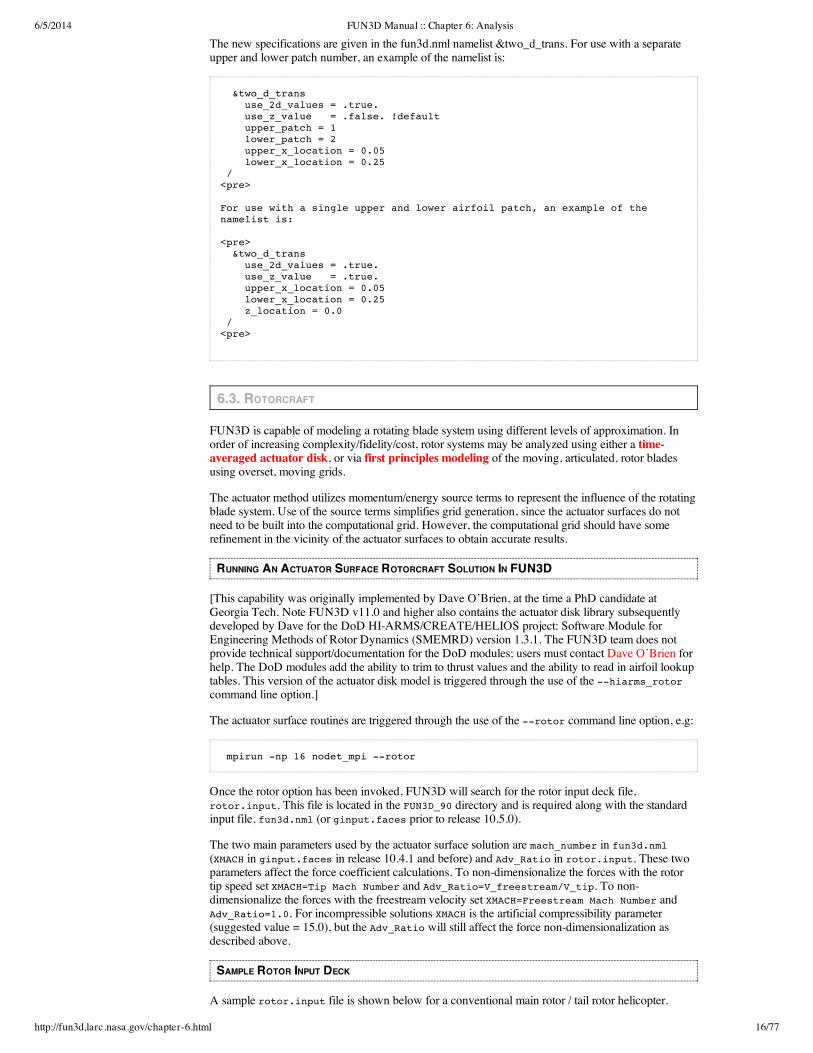
The new specifications are given in the fun3d.nml namelist &two_d_trans. For use with a separateupper and lower patch number, an example of the namelist is:
&two_d_trans use_2d_values = .true. use_z_value = .false. !default upper_patch = 1 lower_patch = 2 upper_x_location = 0.05 lower_x_location = 0.25 /<pre>
For use with a single upper and lower airfoil patch, an example of thenamelist is:
<pre> &two_d_trans use_2d_values = .true. use_z_value = .true. upper_x_location = 0.05 lower_x_location = 0.25 z_location = 0.0 /<pre>
6.3. ROTORCRAFT
FUN3D is capable of modeling a rotating blade system using different levels of approximation. Inorder of increasing complexity/fidelity/cost, rotor systems may be analyzed using either a time-averaged actuator disk, or via first principles modeling of the moving, articulated, rotor bladesusing overset, moving grids.
The actuator method utilizes momentum/energy source terms to represent the influence of the rotatingblade system. Use of the source terms simplifies grid generation, since the actuator surfaces do notneed to be built into the computational grid. However, the computational grid should have somerefinement in the vicinity of the actuator surfaces to obtain accurate results.
RUNNING AN ACTUATOR SURFACE ROTORCRAFT SOLUTION IN FUN3D
[This capability was originally implemented by Dave O’Brien, at the time a PhD candidate atGeorgia Tech. Note FUN3D v11.0 and higher also contains the actuator disk library subsequentlydeveloped by Dave for the DoD HI-ARMS/CREATE/HELIOS project: Software Module forEngineering Methods of Rotor Dynamics (SMEMRD) version 1.3.1. The FUN3D team does notprovide technical support/documentation for the DoD modules; users must contact Dave O’Brien forhelp. The DoD modules add the ability to trim to thrust values and the ability to read in airfoil lookuptables. This version of the actuator disk model is triggered through the use of the --hiarms_rotorcommand line option.]
The actuator surface routines are triggered through the use of the --rotor command line option, e.g:
mpirun -np 16 nodet_mpi --rotor
Once the rotor option has been invoked, FUN3D will search for the rotor input deck file,rotor.input. This file is located in the FUN3D_90 directory and is required along with the standardinput file, fun3d.nml (or ginput.faces prior to release 10.5.0).
The two main parameters used by the actuator surface solution are mach_number in fun3d.nml(XMACH in ginput.faces in release 10.4.1 and before) and Adv_Ratio in rotor.input. These twoparameters affect the force coefficient calculations. To non-dimensionalize the forces with the rotortip speed set XMACH=Tip Mach Number and Adv_Ratio=V_freestream/V_tip. To non-dimensionalize the forces with the freestream velocity set XMACH=Freestream Mach Number andAdv_Ratio=1.0. For incompressible solutions XMACH is the artificial compressibility parameter(suggested value = 15.0), but the Adv_Ratio will still affect the force non-dimensionalization asdescribed above.
SAMPLE ROTOR INPUT DECK
A sample rotor.input file is shown below for a conventional main rotor / tail rotor helicopter.
6/5/2014 FUN3D Manual :: Chapter 6: Analysis
http://fun3d.larc.nasa.gov/chapter-6.html 17/77
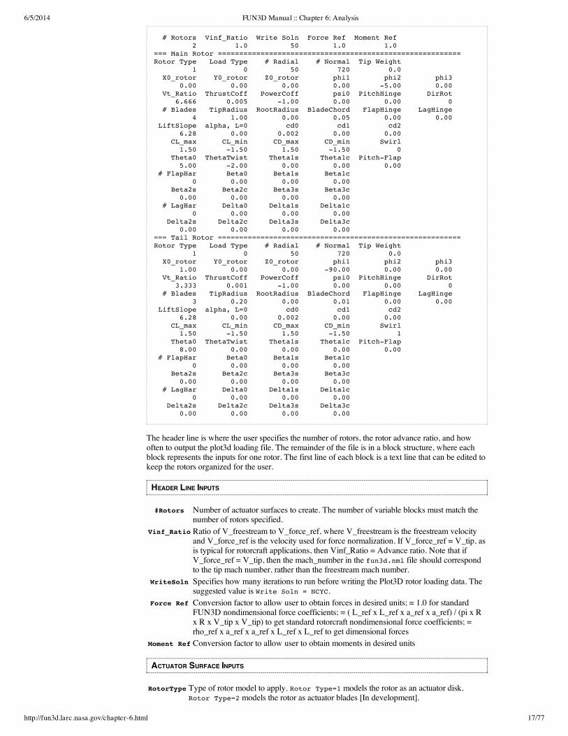
# Rotors Vinf_Ratio Write Soln Force Ref Moment Ref 2 1.0 50 1.0 1.0=== Main Rotor =========================================================Rotor Type Load Type # Radial # Normal Tip Weight 1 0 50 720 0.0 X0_rotor Y0_rotor Z0_rotor phi1 phi2 phi3 0.00 0.00 0.00 0.00 -5.00 0.00 Vt_Ratio ThrustCoff PowerCoff psi0 PitchHinge DirRot 6.666 0.005 -1.00 0.00 0.00 0 # Blades TipRadius RootRadius BladeChord FlapHinge LagHinge 4 1.00 0.00 0.05 0.00 0.00 LiftSlope alpha, L=0 cd0 cd1 cd2 6.28 0.00 0.002 0.00 0.00 CL_max CL_min CD_max CD_min Swirl 1.50 -1.50 1.50 -1.50 0 Theta0 ThetaTwist Theta1s Theta1c Pitch-Flap 5.00 -2.00 0.00 0.00 0.00 # FlapHar Beta0 Beta1s Beta1c 0 0.00 0.00 0.00 Beta2s Beta2c Beta3s Beta3c 0.00 0.00 0.00 0.00 # LagHar Delta0 Delta1s Delta1c 0 0.00 0.00 0.00 Delta2s Delta2c Delta3s Delta3c 0.00 0.00 0.00 0.00=== Tail Rotor =========================================================Rotor Type Load Type # Radial # Normal Tip Weight 1 0 50 720 0.0 X0_rotor Y0_rotor Z0_rotor phi1 phi2 phi3 1.00 0.00 0.00 -90.00 0.00 0.00 Vt_Ratio ThrustCoff PowerCoff psi0 PitchHinge DirRot 3.333 0.001 -1.00 0.00 0.00 0 # Blades TipRadius RootRadius BladeChord FlapHinge LagHinge 3 0.20 0.00 0.01 0.00 0.00 LiftSlope alpha, L=0 cd0 cd1 cd2 6.28 0.00 0.002 0.00 0.00 CL_max CL_min CD_max CD_min Swirl 1.50 -1.50 1.50 -1.50 1 Theta0 ThetaTwist Theta1s Theta1c Pitch-Flap 8.00 0.00 0.00 0.00 0.00 # FlapHar Beta0 Beta1s Beta1c 0 0.00 0.00 0.00 Beta2s Beta2c Beta3s Beta3c 0.00 0.00 0.00 0.00 # LagHar Delta0 Delta1s Delta1c 0 0.00 0.00 0.00 Delta2s Delta2c Delta3s Delta3c 0.00 0.00 0.00 0.00
The header line is where the user specifies the number of rotors, the rotor advance ratio, and howoften to output the plot3d loading file. The remainder of the file is in a block structure, where eachblock represents the inputs for one rotor. The first line of each block is a text line that can be edited tokeep the rotors organized for the user.
HEADER LINE INPUTS
#Rotors Number of actuator surfaces to create. The number of variable blocks must match thenumber of rotors specified.
Vinf_RatioRatio of V_freestream to V_force_ref, where V_freestream is the freestream velocityand V_force_ref is the velocity used for force normalization. If V_force_ref = V_tip, asis typical for rotorcraft applications, then Vinf_Ratio = Advance ratio. Note that ifV_force_ref = V_tip, then the mach_number in the fun3d.nml file should correspondto the tip mach number, rather than the freestream mach number.
WriteSoln Specifies how many iterations to run before writing the Plot3D rotor loading data. Thesuggested value is Write Soln = NCYC.
Force RefConversion factor to allow user to obtain forces in desired units; = 1.0 for standardFUN3D nondimensional force coefficients; = ( L_ref x L_ref x a_ref x a_ref) / (pi x Rx R x V_tip x V_tip) to get standard rotorcraft nondimensional force coefficients; =rho_ref x a_ref x a_ref x L_ref x L_ref to get dimensional forces
Moment RefConversion factor to allow user to obtain moments in desired units
ACTUATOR SURFACE INPUTS
RotorTypeType of rotor model to apply. Rotor Type=1 models the rotor as an actuator disk.Rotor Type=2 models the rotor as actuator blades [In development].
6/5/2014 FUN3D Manual :: Chapter 6: Analysis
http://fun3d.larc.nasa.gov/chapter-6.html 18/77
LoadType Type of loading to apply to the rotor model. Load Type=1 constant pressure jump. LoadType=2 linearly increasing pressure jump. Load Type=3 blade element based loading.Load Type=4 user specified loading.
#Radial Number of sources to distribute along the blade radius. Suggested value is #Radial=100.
#Normal Number of sources to distribute in the direction normal to the radius. Suggested value is# Normal=720 for Rotor Type=1 (one source every 0.5 degrees). Suggested value is #Normal=20 for Rotor Type=2.
TipWeightHyperbolic weighting factor for distributing sources along the blade radius. Input rangeis 0.0 to 2.0, values larger than 2.0 concentrate too many sources at the blade tip.Suggested value is Tip Weight=0.0 (uniform distribution)
ROTOR REFERENCE SYSTEM PLACEMENT AND ORIENTATION
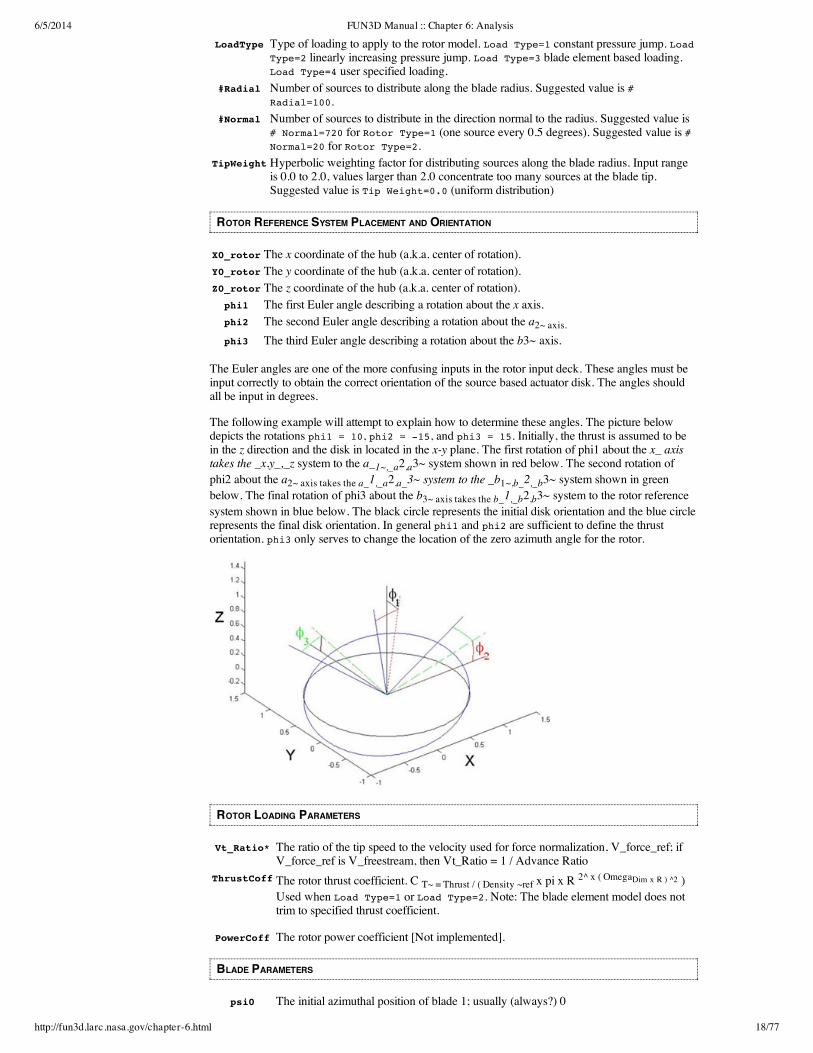
X0_rotorThe x coordinate of the hub (a.k.a. center of rotation).Y0_rotorThe y coordinate of the hub (a.k.a. center of rotation).Z0_rotorThe z coordinate of the hub (a.k.a. center of rotation).phi1 The first Euler angle describing a rotation about the x axis.phi2 The second Euler angle describing a rotation about the a2~ axis.phi3 The third Euler angle describing a rotation about the b3~ axis.
The Euler angles are one of the more confusing inputs in the rotor input deck. These angles must beinput correctly to obtain the correct orientation of the source based actuator disk. The angles shouldall be input in degrees.
The following example will attempt to explain how to determine these angles. The picture belowdepicts the rotations phi1 = 10, phi2 = -15, and phi3 = 15. Initially, the thrust is assumed to bein the z direction and the disk in located in the x-y plane. The first rotation of phi1 about the x_ axistakes the _x,y_,_z system to the a_1~,_a2,a3~ system shown in red below. The second rotation ofphi2 about the a2~ axis takes the a_1,_a2,a_3~ system to the _b1~,b_2,_b3~ system shown in greenbelow. The final rotation of phi3 about the b3~ axis takes the b_1,_b2,b3~ system to the rotor referencesystem shown in blue below. The black circle represents the initial disk orientation and the blue circlerepresents the final disk orientation. In general phi1 and phi2 are sufficient to define the thrustorientation. phi3 only serves to change the location of the zero azimuth angle for the rotor.
ROTOR LOADING PARAMETERS
Vt_Ratio* The ratio of the tip speed to the velocity used for force normalization, V_force_ref; ifV_force_ref is V_freestream, then Vt_Ratio = 1 / Advance Ratio
ThrustCoffThe rotor thrust coefficient. C T~ = Thrust / ( Density ~ref x pi x R 2^ x ( OmegaDim x R ) ^2 )Used when Load Type=1 or Load Type=2. Note: The blade element model does nottrim to specified thrust coefficient.
PowerCoff The rotor power coefficient [Not implemented].
BLADE PARAMETERS
psi0 The initial azimuthal position of blade 1; usually (always?) 0
6/5/2014 FUN3D Manual :: Chapter 6: Analysis
http://fun3d.larc.nasa.gov/chapter-6.html 19/77
PitchHingeThe radial position of the blade pitch hinge (normalized by tip radius).#Blades The number of rotor blades, only used for Load Type=3.TipRadius The radius of the blade.RootRadiusThe radius of the blade root, used to account for the cutout region.BladeChordThe chord length of the blade, only used for Load Type=3. The can only handle
rectangular blade planforms.FlapHinge The radial position of the blade flap hinge (normalized by tip radius).LagHinge The radial position of the blade lag hinge (normalized by tip radius).
BLADE ELEMENT PARAMETERS, ONLY USED WHEN LOAD TYPE=3
LiftSlope;alpha,L=0
Used to compute the lift coefficient.
cd0, cd1, cd2 Used to compute the drag coefficient.CL_max, CL_min Limiters to control the lift coefficient beyond the linear region.CD_max, CD_min Limiters to control the drag coefficient.
Swirl Swirl=0 neglects the sources terms that create rotor swirl. Swirl=1 includes theswirl inducing terms.
CL = LiftSlope x (alpha – alphaL=0)
CD = cd0 + cd1 x alpha + cd2~ x alpha2
PITCH CONTROL PARAMETERS, ONLY USED WHEN LOAD TYPE=3
Theta0 Collective pitch in degrees, defined at r/R=0.ThetaTwistLinear blade twist.Theta1s Longitudinal cyclic pitch input in degrees.Theta1c Lateral cyclic pitch input in degrees.Pitch-FlapPitch-Flap coupling parameter, not implemented.
Theta = Theta0 + ThetaTwist x r/R + Theta1c x cos(psi) + Theta1s x sin(psi)
PRESCRIBED FLAP PARAMETERS
#FlapHar Number of flap harmonics to include, valid input range is 0 to 3Beta0 Coning angle in degrees
Beta1s, Beta1cFist flap harmonicsBeta2s, Beta2cSecond flap harmonicsBeta3s, Beta3cThird flap harmonics
Beta = Beta0 + Beta1s x sin(psi) + Beta1c x cos(psi) + Beta2s x sin(2 psi) + Beta2c x cos(2 psi) +Beta3s x sin(3 psi) + Beta3c x cos(3 psi)
PRESCRIBED LAG PARAMETERS
#LagHar Number of lag harmonics to include, valid input is 0 to 3Delta0 Mean lag angle in degrees
Delta1s, Delta1cFist lag harmonicsDelta2s, Delta2cSecond lag harmonicsDelta3s, Delta3cThird lag harmonics
Delta = Delta0 + Delta1s x sin(psi) + Delta1c x cos(psi) + Delta2s x sin(2 psi) + Delta2c x cos(2psi) + Delta3s x sin(3 psi) + Delta3c x cos(3 psi)
RUNNING AN OVERSET, MOVING MESH ROTORCRAFT SOLUTION IN FUN3D
UNDER CONSTRUCTION
Warning: information incomplete, subject to change, or perhaps even just plain wrong!
This is a very advanced application and it is recommended that the user have experience runningbasic Time Accurate cases and simpler Moving Grid cases without the complications of overset

6/5/2014 FUN3D Manual :: Chapter 6: Analysis
http://fun3d.larc.nasa.gov/chapter-6.html 20/77
meshes.
Overset grid applications require the SUGGAR++ and DiRTlib libraries developed by RalphNoack. The user should gain experience with the SUGGAR++ code for simpler overset cases beforeembarking on the more complex rotorcraft problem.
Overset, moving mesh rotorcraft solutions can be divided into those involving rigid blades and thoseinvolving flexible (aeroelastic) blades. The latter case is quite complex, and requires the use of a“comprehensive” rotorcraft structural dynamics (CSD) code such as CAMRAD II or Dymore .The CSD code provides the structural model for the blade deformation, and furnishes trim algorithmsfor determining the basic rotor settings such as the collective and cyclic pitch angles. Currently, onlythe “loose coupling” approach has been implemented, limiting the analysis to hover or steady levelflight.
BASIC STEPS – RIGID BLADES
The following are the primary steps required to run a rotorcraft simulation in which the blades aretreated as being rigid.
1) Set up the rotor.input and moving_body.input files2) Generate the component fuselage/background and rotor blade VGRID meshes3) (Optional) Set up the &slice_data namelist in the fun3d.nml file to extract airloads data along thereference blade4) Generate the composite mesh with the rotor blades in the t=0 position using the dci_gen utilitycode
6) Run the flow solver for one rotor revolution, using --dci_on_the_fly to generate the oversetconnectivity files; you may optionally use—dci_period NP for this first run (required for subsequentruns), where NP is the number of time steps taken to complete one revolution (e.g. 360 for 1 deg.motion per time step)7) Run the flow solver for a number of additional rotor revolutions, either without --dci_on_the_fly (i.e reuse the dci from step 6), or with --reuse_existing_dci in addition to --dci_on_the_fly; you also need to use —dci_period NP for any revolution beyond the first one,where NP is the number of time steps taken to complete one revolution8) (Optional) Post process the rotor airloads data from step 3 using the process_rotor_data utilitycode
Note: Steps 6) and 7) above can be combined into a single run by first ensuring that the only dci filein the run directory is the initial one (i.e. the [project].dci file), and then using the combination --dci_on_the_fly --reuse_existing_dci --dci_period NP command-line options. This willcreate the required dci files during the first revolution (since they don’t exist), and then reuse them onsubsequent revolutions. If the --reuse_existing_dci command-line option is omitted, new dci fileswill be generated each revolution (unnecessary for rigid blades undergoing cyclic motion).
In addition to the command-line options for the flow solver given above, all overset, moving-grid,rigid-blade rotorcraft cases with FUN3D will also require
--moving_grid --overset_rotor
And one may also choose to use (optional steps 3 and 8 above)
--slice_freq 1 --output_comprehensive_loads
BASIC STEPS – ELASTIC BLADES
The following are the primary steps required to run a rotorcraft simulation in which the blades aretreated as being elastic, and thus the flow solver is coupled to an external CSD code.
1) Set up the rotor.input and moving_body.input files2) Generate the component fuselage/background and rotor blade VGRID meshes3) Set up the &slice_data namelist in the fun3d.nml file to extract airloads data along the referenceblade (Required)4) Generate the composite mesh with the rotor blades in the t=0 position5a) Set up and run the comprehensive rotorcraft code to generate reference motion data5b) Set up and run the comprehensive rotorcraft code using only the comprehensive code’s built-inlinear aerodynamics model5c) Generate a blade motion file from the comprehensive code data6a) Run the flow solver for 1 rotor revolutions, using --dci_on_the_fly to generate the overset

6/5/2014 FUN3D Manual :: Chapter 6: Analysis
http://fun3d.larc.nasa.gov/chapter-6.html 21/77
connectivity files; you may optionally use—dci_period NP for this first run (required for subsequentruns), where NP is the number of time steps taken to complete one revolution (e.g. 360 for 1 deg.motion per time step)6b) Run the flow solver for 1-2 additional revolutions, either without --dci_on_the_fly (i.e reusethe dci from step 6a), or with --reuse_existing_dci in addition to --dci_on_the_fly and --dci_period NP
7a) Generate a “delta airloads” file for the comprehensive rotorcraft code7b) Set up and run the comprehensive rotorcraft code using the current “delta airloads”8) Go back to step 5c and repeat until “delta airloads” converge and trim targets are met; onsubsequent cycles through step 6, run the flow solver for 2/Nblades revolutions each time, using --dci_on_the_fly (i.e. recompute the dci data) and --dci_period NP
Note: The first pass through Steps 6a) and 6b) above can be combined into a single run by firstensuring that the only dci file in the run directory is the initial one (i.e. the [project].dci file), and thenusing the combination --dci_on_the_fly --reuse_existing_dci --dci_period NP command-line options. This will create the required dci files during the first revolution (since they don’t exist),and then reuse them on subsequent revolutions. Note that for subsequent coupling cycles, for whichonly partial revolutions are completed in a given run, do not use --reuse_existing_dci, as new dcifiles are needed when the blade motion/shape changes.
In addition to the command-line options for the flow solver given above, all overset, moving-grid,elastic-blade rotorcraft cases with FUN3D will also require
--moving_grid --overset_rotor --comprehensive_rotor_coupling 'camrad' --slice_freq 1
For elastic/coupled blade analysis, a sample PBS run script RUN_LOOSE_COUPLING is provided in theutils/Rotorcraft directory. This script removes much of the tedium of running a coupled rotorcraftanalysis “by hand” as outlined above. The run script is set up to work with the CAMRAD IIcomprehensive code, although the changes to the script to work with other comprehensive codesshould be relatively minor.
Aerodynamic data from FUN3D to the comprehensive code is provided via the FUN3D output filerotor_N.onerev.txt (N the rotor number). This file has the same form and function as thecorresponding file that is output from the OVERFLOW code.
Blade motion data to FUN3D from the comprehensive code is provided via the FUN3D input filecamrad_motion_data_rotor_N.dat (N the rotor number). Despite the name difference, this file hasthe same form and function as the motion.txt file used by the OVERFLOW code.
Note that CAMRAD does not directly use the rotor_N.onerev.txt file. To utilize therotor_N.onerev.txt file to generate the “delta airloads” file actually used by CAMRAD, anintermediate translation code is required. Likewise, CAMRAD does directly output thecamrad_motion_data_rotor_N.dat file needed by FUN3D; again, an intermediary code isrequired. Suitable intermediary codes (gen_delta_for_cii and gen_motion_for_cfd) have beenwritten for OVERFLOW/CAMRAD coupling and can be used with FUN3D/CAMRAD as well.These intermediary codes may be requested from:
Doug Boyd (NASA Langley Aeroacoustics Branch)
The RUN_LOOSE_COUPLING script relies on the above-mentioned conversion codes.
UTILITY CODES / SCRIPTS / FILES
The FUN3D suite includes several utility codes in the utils/Rotorcraft directory:
dci_gen.f90 Uses (lib)SUGGAR++ to create a composite rotorcraft mesh fromcomponent rotor blade and fuselage/background grids
dci_gen.input A sample input file for the dci_gen codeRUN_DCI_PARALLEL A run script for the dci_gen code
process_rotor_data.f90Reads the rotor_N.onerev.txt file and correspondingmotion_rotor_N.onerev.txt file and generates Tecplot files forplotting airloads and motion data
RENUMBER_DCI_FILES A script to renumber existing dci files so that a set of dci files generatedfor one time step can be reused with a different time step
RUN_LOOSE_COUPLING A script to run a loosely coupled CFD/CSD elastic-blade rotorcraftsimulation
hart2_ref.scr Sample CAMRAD run scripts set up for compatibility with the

6/5/2014 FUN3D Manual :: Chapter 6: Analysis
http://fun3d.larc.nasa.gov/chapter-6.html 22/77
hart2_0.scrhart2_n.scr
RUN_LOOSE_COUPLING script
SUBSET OF ROTOR.INPUT VARIABLES USED FOR “FIRST PRINCIPLES” ROTORCRAFT CASES
Of the parameters in the rotor.input file described above, only the following are needed foroverset, moving mesh cases; zeroes may be entered for all other values. Note that for flexible-bladesimulations the pitch, flap and lag harmonics are not used, although the pitch, flap and lag hingelocations are used. For flexible-blade simulations, the pitch, flap and lag motions are accounted for inthe motion file provided (indirectly) by the comprehensive rotorcraft code.
No. Rotors, Vinf_Ratio
X0_Rotor, Y0_Rotor, Z0_Rotor
phi2
Vt_Ratio, PitchHinge
No. Blades, TipRadius, RootRadius, BladeChord, FlapHinge, LagHinge
Theta0, Theta1s, Theta1c (ignored for elastic blades)
No. FlapHar, Beta0, Beta1s, Beta1c (ignored for elastic blades)
Beta2s, Beta2c, Beta3s, Beta3c (ignored for elastic blades)
No. LagHar Delta0, Delta1s, Delta1c (ignored for elastic blades)
Delta2s, Delta2c, Delta3s, Delta3c (ignored for elastic blades)
ROTATION SPEED AND TIME STEP
In the discussion below, it is assumed that the geometry represented by the grid is unscaled relative tothe actual configuration; e.g. if the actual rotor radius is 26.833 ft., then the corresponding rotor radiusin the grid used for computations is also 26.833.
The non-dimensional rotor rotation rate is not set directly by the user, but rather via a combination ofVt_Ratio and TipRadius values in the rotor.input file, and the mach_number value in thefun3d.nml file:
omega = vt_ratio x mach_number / r_tip (compressible flow)
omega = vt_ratio / r_tip (incompressible flow)
where omega is in radians (per unit nondimensional time).
To set the value of time_step_nondim in the fun3d.nml input file, first decide on the desiredazimuthal resolution for each time step, dpsi. A value of dpsi of 1 degree per time step is usually areasonable starting point.
The nondimensional time step may be determined using
dpsi = omega x time_step_nondim x 180 / pi
So that
time_step_nondim = dpsi x pi / 180 x r_tip / vt_ratio / xmach (compressible)
time_step_nondim = dpsi x pi / 180 x r_tip / vt_ratio (incompressible)
Tip: As a check, the resulting non-dimensional rotation rate and azimuth change per time step areoutput to the screen in the “Rotor info” section. Make sure this output value matches your desiredvalue to a fair degree of precision, to ensure that the rotor blades are accurately positioned at eachtime step. Inaccuracies can occur if, for example, you base your calculation of time_step_nondim on avalue of r_tip = 26.8330 but in the rotor.input file you have a value of r_tip = 26.8333
SUBSET OF MOVING_BODY.INPUT VARIABLES USED FOR “FIRST PRINCIPLES” ROTORCRAFT CASES
As with all moving body simulations, a moving_body.input file is required. However, themoving_body.input file for rotorcraft cases is primarily used to define the moving bodies (the rotorblades) as particular boundary surfaces within the mesh, while the blade motion is specified in the
6/5/2014 FUN3D Manual :: Chapter 6: Analysis
http://fun3d.larc.nasa.gov/chapter-6.html 23/77
rotor input deck described above . The value of Vt_ratio sets the rotation rate of the rotor while thevalues of the theta, beta, and delta variables set the pitch, flap and lag motions of the blades. Note: forelastic blades, the pitch, flap and lag motions are not set via the rotor.input file, but rather via aseparate “blade motion” file; Vt_ratio does set the rotation rate, however. This differs from the usualmoving body case wherein the body motion is specified in the moving_body.input file. Forrotorcraft cases, the motion_driver variable should not not be specified in the &body_definitionsnamelist, and the &forced_motion namelist should be omitted entirely.
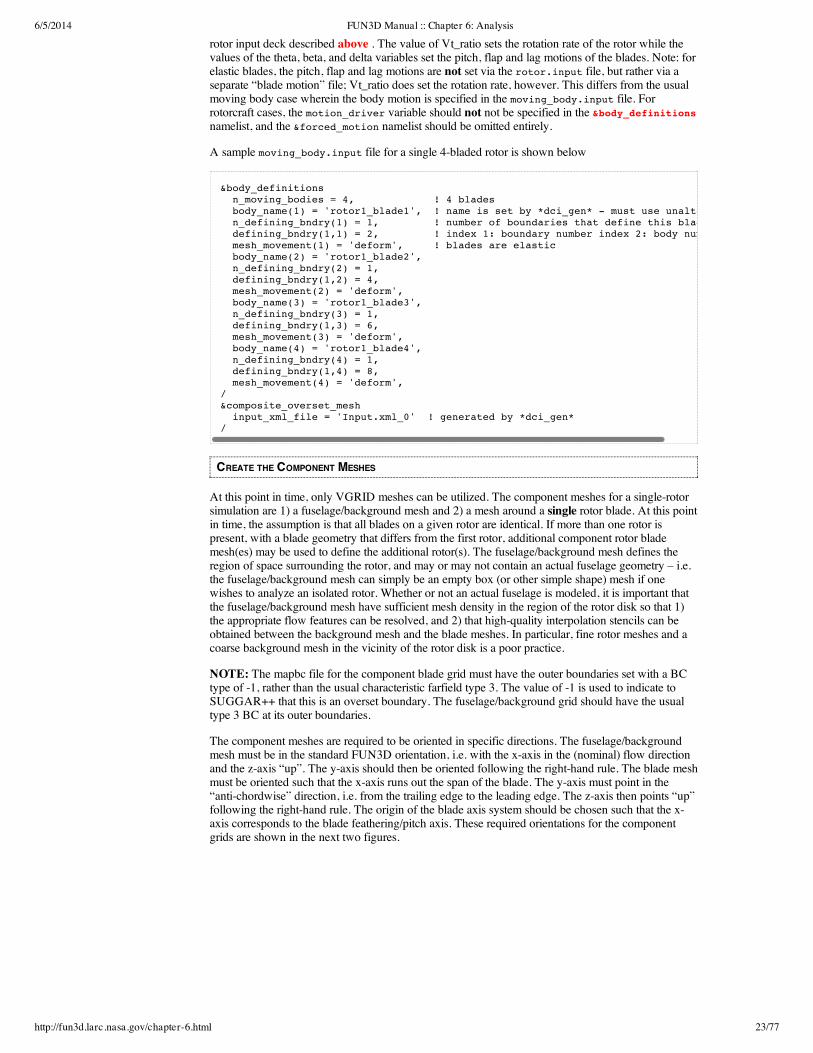
A sample moving_body.input file for a single 4-bladed rotor is shown below
CREATE THE COMPONENT MESHES
At this point in time, only VGRID meshes can be utilized. The component meshes for a single-rotorsimulation are 1) a fuselage/background mesh and 2) a mesh around a single rotor blade. At this pointin time, the assumption is that all blades on a given rotor are identical. If more than one rotor ispresent, with a blade geometry that differs from the first rotor, additional component rotor blademesh(es) may be used to define the additional rotor(s). The fuselage/background mesh defines theregion of space surrounding the rotor, and may or may not contain an actual fuselage geometry – i.e.the fuselage/background mesh can simply be an empty box (or other simple shape) mesh if onewishes to analyze an isolated rotor. Whether or not an actual fuselage is modeled, it is important thatthe fuselage/background mesh have sufficient mesh density in the region of the rotor disk so that 1)the appropriate flow features can be resolved, and 2) that high-quality interpolation stencils can beobtained between the background mesh and the blade meshes. In particular, fine rotor meshes and acoarse background mesh in the vicinity of the rotor disk is a poor practice.
NOTE: The mapbc file for the component blade grid must have the outer boundaries set with a BCtype of -1, rather than the usual characteristic farfield type 3. The value of -1 is used to indicate toSUGGAR++ that this is an overset boundary. The fuselage/background grid should have the usualtype 3 BC at its outer boundaries.
The component meshes are required to be oriented in specific directions. The fuselage/backgroundmesh must be in the standard FUN3D orientation, i.e. with the x-axis in the (nominal) flow directionand the z-axis “up”. The y-axis should then be oriented following the right-hand rule. The blade meshmust be oriented such that the x-axis runs out the span of the blade. The y-axis must point in the“anti-chordwise” direction, i.e. from the trailing edge to the leading edge. The z-axis then points “up”following the right-hand rule. The origin of the blade axis system should be chosen such that the x-axis corresponds to the blade feathering/pitch axis. These required orientations for the componentgrids are shown in the next two figures.
&body_definitions n_moving_bodies = 4, ! 4 blades body_name(1) = 'rotor1_blade1', ! name is set by *dci_gen* - must use unaltered n_defining_bndry(1) = 1, ! number of boundaries that define this blade defining_bndry(1,1) = 2, ! index 1: boundary number index 2: body number mesh_movement(1) = 'deform', ! blades are elastic body_name(2) = 'rotor1_blade2', n_defining_bndry(2) = 1, defining_bndry(1,2) = 4, mesh_movement(2) = 'deform', body_name(3) = 'rotor1_blade3', n_defining_bndry(3) = 1, defining_bndry(1,3) = 6, mesh_movement(3) = 'deform', body_name(4) = 'rotor1_blade4', n_defining_bndry(4) = 1, defining_bndry(1,4) = 8, mesh_movement(4) = 'deform',/&composite_overset_mesh input_xml_file = 'Input.xml_0' ! generated by *dci_gen*/

6/5/2014 FUN3D Manual :: Chapter 6: Analysis
http://fun3d.larc.nasa.gov/chapter-6.html 24/77

6/5/2014 FUN3D Manual :: Chapter 6: Analysis
http://fun3d.larc.nasa.gov/chapter-6.html 25/77
CREATE THE COMPOSITE MESH
A utility code, dci_gen, is provided with the FUN3D suite of codes, in the utils/Rotorcraftdirectory. Compiling of the utility code is performed with a top-level “make” in your configurationdirectory; alternatively in the configuration directory, cd to utils/Rotorcraft and type make there.NOTE you will have had to configure with the --with-suggar option (see SUGGAR++).
Before using dci_gen, the rotor.input file should be set up. For rigid-blade analysis, thecollective/cyclic data in rotor.input is used to position the blades in the composite mesh at thecorrect orientation at t=0. If this is a simulation with elastic blades, an initial “motion.txt” file mustalso be available. For those familiar with the OVERFLOW code for rotorcraft applications, this is thesame file, with the same format, as used with OVERFLOW. However, with FUN3D, this initial“motion.txt” file must have a very specific name (at the time of writing):camrad_motion_data_rotor_N_t0.dat (N the rotor number). The required motion file may be theresult from an initial comprehensive code analysis using the CSD code’s internal aerodynamicsmodule, i.e. the initial step in a coupled CFD/CSD coupling. In this case additional motion files willgenerated later as the coupling progresses. Alternatively, you may have a final motion file resultingfrom some other process; in this case you will have only one motion file, but that motion file must stillbe named camrad_motion_data_rotor_N_t0.dat for dci_gen. In the case of elastic blades, theorientation of the blades at t=0 is determined from this initial motion file, rather than from therotor.input file.
Upon execution, dci_gen will prompt the user for input:
1) a project name (for the assembled, composite grid)2) the name of the VGRID component fuselage grid3) the name of the VGRID component blade grid for the first rotor (if multiple rotors, additionalcomponent blade grid names will be requested)4) the initial_azimuth, final_azimuth and azimuthal_increment

6/5/2014 FUN3D Manual :: Chapter 6: Analysis
http://fun3d.larc.nasa.gov/chapter-6.html 26/77
5) whether or not the blades are considered rigid6) if more that one rotor was specified, the gear ratio to rotor 1 for each additional rotor
If the blades are rigid, then the specified final_azimuth could larger than the initial_azimuth (somemultiple of the increment), and dci_gen would generate multiple dci files, one for each azimuth.There is even a provision for doing so in parallel. However, the easiest process, and the only onedescribed here, is to set initial_azimuth = final_azimuth = 0. In this case, only one dci file isgenerated, corresponding to psi = 0. Subsequent dci files are then generated “on the fly” whenrunning running FUN3D. For elastic blades, this is the only approach available (i. e. only the psi=0dci file created up front, others computed “on the fly”)
dci_gen will read your rotor.input file (and if elastic, the “motion.txt” file), take the componentVGRID meshes that you specify, and create SUGGAR++ xml commands to position the blade gridat appropriate locations and orientations around the rotor disk (e.g. at 90 deg. locations for a 4-bladedrotor, with appropriate pitch settings, etc.). This xml file will be named Input.xml_0, and is the xmlfile that should be specified as the input_xml_file in the &composite_overset_mesh namelist ofthe moving_body.input file. dci_gen will then use (lib)SUGGAR++ to generate both a compositemesh and the corresponding dci file for the rotor in the initial position, at t=0. In the composite mesh,blade 1 will be aligned with the axis of the fuselage (the x-axis), as shown below.
dci_gen will also set up a mapbc file for the composite grid. In this mapbc file you should find/verifythat the BCs from the original blade component grid have been replicated nblade times, and inparticular the overset BC (-1) should appear for each blade. The family names of the blade and outerboundaries will be prepended by rotorN_ (N the rotor number) and appended by the blade number.For example, if the family name for the blade surfaces in the blade component grid was “Blade”, thenin the composite mapbc file, the blades will have family names “rotor1_Blade1”, rotor1_Blade2”, etc.The BCs and family names of the fuselage/background grid will be unchanged from the component-grid mapbc file.
Domain connectivity files (dci files) will be generated for each azimuthal angle psi from the initial tothe final value, with the specified increment. A composite mesh is generated only if the initial psivalue is zero.
Below is the resulting 4-bladed composite geometry created from the blade and fuselage componentgeometries shown above.
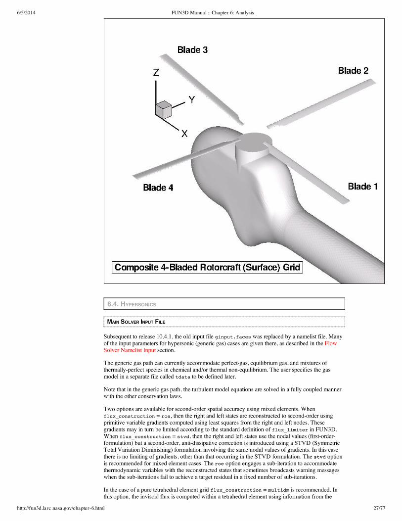
6/5/2014 FUN3D Manual :: Chapter 6: Analysis
http://fun3d.larc.nasa.gov/chapter-6.html 27/77
6.4. HYPERSONICS
MAIN SOLVER INPUT FILE
Subsequent to release 10.4.1, the old input file ginput.faces was replaced by a namelist file. Manyof the input parameters for hypersonic (generic gas) cases are given there, as described in the FlowSolver Namelist Input section.
The generic gas path can currently accommodate perfect-gas, equilibrium gas, and mixtures ofthermally-perfect species in chemical and/or thermal non-equilibrium. The user specifies the gasmodel in a separate file called tdata to be defined later.
Note that in the generic gas path, the turbulent model equations are solved in a fully coupled mannerwith the other conservation laws.
Two options are available for second-order spatial accuracy using mixed elements. Whenflux_construction = roe, then the right and left states are reconstructed to second-order usingprimitive variable gradients computed using least squares from the right and left nodes. Thesegradients may in turn be limited according to the standard definition of flux_limiter in FUN3D.When flux_construction = stvd, then the right and left states use the nodal values (first-order-formulation) but a second-order, anti-dissipative correction is introduced using a STVD (SymmetricTotal Variation Diminishing) formulation involving the same nodal values of gradients. In this casethere is no limiting of gradients, other than that occurring in the STVD formulation. The stvd optionis recommended for mixed element cases. The roe option engages a sub-iteration to accommodatethermodynamic variables with the reconstructed states that sometimes broadcasts warning messageswhen the sub-iterations fail to achieve a target residual in a fixed number of sub-iterations.
In the case of a pure tetrahedral element grid flux_construction = multidm is recommended. Inthis option, the inviscid flux is computed within a tetrahedral element using information from the
6/5/2014 FUN3D Manual :: Chapter 6: Analysis
http://fun3d.larc.nasa.gov/chapter-6.html 28/77
three-dimensional stencil of nodes defining the element. It provides far superior results for heating andshear across high aspect ratio tetrahedral cells than any of the edge-based reconstruction methodstested to date. Heating and shear are still best simulated using a semi-structured grid across theboundary layer and orthogonal to the wall – but if such a grid is not available it is recommended toconvert the grid to a pure tets using the command line option --make_tets and useflux_construction = multidm.
Mach number and Reynolds number per grid unit are computed from the fundamental inputs ofvelocity, density, and temperature.
If a non-constant wall temperature boundary condition is specified (see Boundary Conditions forGeneric Gas Option) then the parameter temperature_walldefault serves only to initialize thesurface boundary condition.
The flag chemical_kinetics is engaged only in the case of multiple species defined in file tdata. Ifchemical_kinetics is set to frozen for chemically frozen flow then the chemical source term isnever called and species mass fractions can only be changed through the action of diffusion. If it is setto finite-rate for chemically reacting flow then the chemical source term is called and speciesmass fractions change by kinetic action of dissociation, recombination, ionization, and de-ionization.The flag thermal_energy_model is set to frozen for thermally frozen flow or to non-equilib forthermally active flow (flow in thermal non-equilibrium). This flag is engaged only when a thermalnon-equilibrium model is specified in the file tdata; otherwise thermal equilibrium is assumed. If it isset to frozen for thermally frozen flow then the thermal energy exchange source term is never calledand the modeled modal temperatures (vibrational, electronic) can be changed only by the action ofconduction. (Translational temperature still evolves through the action of flow work but this energy isnever transferred to internal energy modes.) If it is set to non-equilib then the source term modelsparticle collisions in which particle internal energy in the translational, rotational, vibrational, andelectronic modes can be exchanged.
The parameter invis_relax_factor is a relaxation factor on the update, dq, to the conservativeflow variables q. Before an update, dq is divided by the maximum value of five limiting factorsincluding invis_relax_factor. The first four limiting factors are computed internally and designedto limit the rate of change of pressure, density, temperature, and velocity. If invis_relax_factor isset to 1.0, no further limiting is engaged. The parameter visc_relax_factor is a relaxation factorthat multiplies only the viscous Jacobian. Its value should be set to 1.0; it is retained here as a placeholder for future research. The parameter rhs_u_eigenvalue_coef is the eigenvalue limiter. It actsonly on the evaluation of the eigenvalues used on the right-hand-side convective portion of theresidual using Roe’s method. If eigenvalues are less than rhs_u_eigenvalue_coef times the localsound speed then a formula due to Harten is employed to smoothly limit the eigenvalue. Numericaltests show that the heating and solution quality near the wall are severely compromised usingeigenvalue limiting when tetrahedra are used throughout. The parameter value should be set to 1.e-30 (it must be positive definite) in this case. It is retained as an input parameter in case it is needed, asin the structured grid approach of LAURA, when prismatic elements are introduced. The parameterlhs_u_eigenvalue_coef is also an eigenvalue limiter but is applied only in the evaluation of theinviscid Jacobian (left-hand-side) by Roe’s method. Recommended values between .001 and 1.0provide a more well-determined matrix. Larger values enhance robustness with the possible penaltyof slower convergence, particularly in stagnation regions.
GAS MODEL INPUT FILE: TDATA
The file tdata defines the gas model. Information in this file is likely to change from one applicationto another, depending on the flow regime, velocity, and atmospheric composition. It contains a list ofkey words, sometimes followed by numeric values, which identify components of the gas model.One or more spaces must separate keyword and values when appearing on the same line. Spaces mayappear to the left or right of any key word. The first line of the file must not be blank. Options forperfect-gas, equilibrium gas, and mixtures of thermally perfect gases can be accommodated. Anexample of the input data file tdata used for each will be presented.
PERFECT GAS
The perfect-gas option is engaged with any of the following keywords: perfect_gas, PERFECT_GAS,Perfect_Gas, Perfect_gas.
If no further data is provided in this file, this single line tdata file will assume the followingparameter values in SI units for air:
gamma 1.4 mol_wt 28.8 suther1 0.1458205E-05 suther2 110.333333 prand 0.72

6/5/2014 FUN3D Manual :: Chapter 6: Analysis
http://fun3d.larc.nasa.gov/chapter-6.html 29/77
Here, gamma is the gas specific heat ratio, mol_wt is the gas molecular weight, prand is the gasPrandtl number, and suther1 and suther2 are the first and second Sutherland’s viscositycoefficients where
mu = suther1*T**(3/2)/(T +suther2)
These values can be modified and explicitly defined in the tdata using the species_propertiesnamelist by placing the keyword &species_properties in the second line of tdata followed by thegas parameters and / at the last line of the file. For example,
perfect_gas &species_properties gamma = 1.4 mol_wt = 28.0 suther1 = 0.1E-05 suther2 = 110.3 prand = 0.7 /
EQUILIBRIUM GAS
To engage the Tannehill curve fits for thermodynamic and transport properties of equilibrium air thefollowing keyword should be used in the first line of the tdata file:
equilibrium_air_t
To use a table look-up capability for equilibrium gases the following keyword should be placed in thetdata file:
equilibrium_air_r
Table look-up data for air is contained in the files eq_air_coeffs.asc and eq_air_lk_up.ascwhich may be found in the PHYSICS_MODULES directory. Note that this option still uses the Tannehilltransport properties. No additional inputs or files are required to engage the Tannehill option forequilibrium air.
MIXTURE OF THERMALLY PERFECT GASES
two N2 .767 N O2 .233 O NO H2 N2 H2O H OH
The first entry of the file may contain an optional flag which identifies the thermal model. If nothermal flag is present or if the flag says one, One, or ONE then the gas is in thermal equilibrium (aone-temperature model). If there is no thermal flag then the first line of this file must contain speciesinformation as described in the next paragraph; this file cannot begin with a blank line. If the flag saystwo, Two, or TWO then the gas is modeled using a two-temperature model. The two temperature modelassumes energy distribution in the translational and rotational modes of heavy particles (not electrons)are equilibrated at temperature T and all other energy modes (vibrational, electronic, electrontranslational) are equilibrated at temperature $T_V$. No other thermal models are currently available;however, the source code is written to accommodate an arbitrary number of additional thermaldegrees of freedom.
Subsequent file entries include species names, appearing exactly as defined in the master data filespecies_thermo_data (see below). If a value appears to the right of the species name, separated byone or more spaces, then that value denotes the mass fraction of the species at an inflow boundary. Ifno value appears to the right of the species name then that species is not present on inflow but may beproduced through chemical reactions elsewhere in the flow field.

6/5/2014 FUN3D Manual :: Chapter 6: Analysis
http://fun3d.larc.nasa.gov/chapter-6.html 30/77
Multiple instances of inflow boundaries can be accommodated. However, this option is not yet beenexercised. For example, air may flow in from an inlet boundary and fuel may flow in from a separateinflow port. A blank line (line (7) in the example) separates instances of inflow boundary conditions.If new species are introduced in subsequent instances they are automatically initialized to zero at anyprevious inflow boundary. They are also available as a reactant throughout the entire flow field.
THERMODYNAMIC DATA INPUT FILE
The file species_thermo_data is the master file for species thermodynamic data. Here is a sample.
C &species_properties molecule = .false. ion = .false. elec_impct_ion = 11.264 ! Moore ? 4.453 in mars.F siga = 7.5e-20, 5.5e-24, -1.e-28 mol_wt = 12.01070 / 3 0.64950315E+03 -0.96490109E+00 0.25046755E+01 -0.12814480E-04 0.19801337E-07 -0.16061440E-10 0.53144834E-14 0.00000000E+00 0.85457631E+05 0.47479243E+01 200.000 1000.000 -0.12891365E+06 0.17195286E+03 0.26460444E+01 -0.33530690E-03 0.17420927E-06 -0.29028178E-10 0.16421824E-14 0.00000000E+00 0.84105978E+05 0.41300474E+01 1000.000 6000.000 0.44325280E+09 -0.28860184E+06 0.77371083E+02 -0.97152819E-02 0.66495953E-06 -0.22300788E-10 0.28993887E-15 0.00000000E+00 0.23552734E+07 -0.64051232E+03 6000.000 20000.000 gamma_air &species_properties molecule = .true. ion = .false. mol_wt = 28.8 suther1 = 0.1458205E-05 suther2 = 110.333333 prand = 0.7 / 1 0.00000000E+00 0.00000000E+00 0.10000000E+01 0.00000000E+00 0.00000000E+00 0.00000000E+00 0.00000000E+00 0.00000000E+00 0.00000000E+00 0.00000000E+00 0.0 100000.000
A species record consists of the species name, a species properties namelist, the number ofthermodynamic property curve fit ranges, and the curve fit coefficients for each range.[1]
1 B. J. McBride and S. Gordon, “Computer Program for calculation of Complex ChemicalEquilibrium Compositions and Applications”, NASA RP 1311, June 1996.
6.5. TIME ACCURATE – BASICS/FIXED GEOMETRY
INTRODUCTION
The basic input parameters for running fixed-mesh, time-dependent cases, are described under FlowSolver Input Deck . This section describes other essential information needed to run fixed-meshtime-dependent cases, and time-dependent cases in which the geometry moves.
NondimensionalizationTemporal Order of AccuracyTemporal Error ControllerAnimation of Unsteady Flows
NONDIMENSIONALIZATION
A description of the nondimensionalization is under construction; in the interim, the description givenin the CFL3D documentation will suffice. For compressible flows, the two codes use exactly thesame nondimensionalization. Note that for incompressible flow (for which CFL3D has nocounterpart), the reference velocity is the freestream velocity, rather than the freestream speed ofsound.
TEMPORAL ORDER OF ACCURACY

6/5/2014 FUN3D Manual :: Chapter 6: Analysis
http://fun3d.larc.nasa.gov/chapter-6.html 31/77
Currently, the available time-advancement schemes in FUN3D are multistep, backward difference(BDF) schemes. Second-order accuracy (itime = 2) has been the order of choice for a long time,although in Version 10.0, third order (itime = 3) and an “in between” second and third order scheme(“BDF2opt”, itime = -3) were added. Note that the third-order scheme is not guaranteed to be stable;in practice this is usually not a problem, but in a few cases the lack of guaranteed stability has lead tosolutions which diverge after a very long time. The BDF2opt is guaranteed to be stable and hence isrecommended if accuracy higher than second order in time is needed. Bear in mind that for practicalapplications, solution accuracy is likely to be limited by low grid resolution, so a high-order timeadvancement may not lead to improved overall accuracy. First order accuracy in time is rarely used.A possible exception being to reproduce steady state convergence while running in unsteady mode –as may be needed for static aeroelastic applications, for example. With a very large time step (e.g.1.e20) and first-order time accuracy (itime=1), the time-accurate path will converge exactly as thesteady state path (itime=0).
TEMPORAL ERROR CONTROLLER
The name is somewhat misleading, in that this controller addresses one source of temporal errors,namely, insufficient subiterations. As described in the Flow Solver Input Deck section, the usermust specify the number of subiterations in pseudo time in between each physical time step. Ideally,enough subiterations should be used to converge the mean flow and turbulence residuals to machinezero. That of course is prohibitively expensive, so a more reasonable number of subiterations must beused. The question then is, how many subiterations are enough? It has also been observed that acertain points during unsteady simulations, subiterations converge faster, and conversely slower atother times in the simulation. Using a fixed number of subiterations sufficient for the harder portionsmeans there will be an excess of iterations on the easier portions, thereby wasting CPU time.
The temporal error control options seeks to mitigate these issues by providing a well-founded cutoff.When using the controller, a reasonably large number of subiterations is specified, perhaps 25 to 75.The error controller itself is invoked with the command line option
--temporal_err_control TOL
where TOL is a real valued tolerance. Limited calibration studies suggest a value of 0.05 to 0.1 isreasonable. When run with this command line option, the solver will obtain an estimate of thetemporal error, and when the x-momentum and turbulence residuals drop below TOL times theestimated error, the subiteration loop will terminate. If the tolerance is not reached by the end of thespecified number of subiterations, a warning message is printed.
ANIMATION OF UNSTEADY FLOWS
This information has been moved to Flow Visualization Output Directly From Flow Solver
6.6. TIME ACCURATE – MOVING GEOMETRY
INTRODUCTION
This section describes the capability for simulating flows with moving/changing geometry. It isstrongly recommended that the user become familiar with time-dependent stationary-geometrysimulations before attempting moving-geometry cases.
Moving Bodies/Grids – General InformationPost-Processing/Repartitioning Moving Grid CasesDefining Moving BodiesSpecified Body MotionSpecified Observer Motion (for animation)Body Motion via File Input6DOF MotionAeroelastic Motion (Mode Based)Sample moving_body.input FilesMesh Deformation
MOVING BODIES/GRIDS – GENERAL INFORMATION
NOTE: this is an active area of development, so implementation or input details may changewith time.

6/5/2014 FUN3D Manual :: Chapter 6: Analysis
http://fun3d.larc.nasa.gov/chapter-6.html 32/77
The ability to move the grid as a rigid body (no deformation) was introduced in Version 10.0; priorversions have no provisions for moving geometries. Later versions have increased capability fordeforming meshes, thereby allowing some distinction between “body motion” and “grid motion”.The current nomenclature is such that one specifies the motion of a “body” (a collection of one ormore solid surfaces within the grid), and associates with that body a mechanism for moving thesurrounding grid points – either rigidly, so that all points move in concert with the body, or in adeforming manner so that points near the body move in concert with the body, but points far awaymove little, if at all.
Grid motion is enabled via the command line option
--moving_grid
In addition to this command line option, an additional file is required to specify the details of the bodymotion, and to specify how the grid is moved to accommodate the motion of the body.
The --moving_grid command line and moving_body.input file are also required for postprocessingmoving grid solutions with party. Contrary to earlier versions of the flow solver, the part files are notmodified as the grid is moved. Thus the part files always contain the grid at is was at t=0; the restart(flow) files now contain the mesh coordinates for the current position. Thus it is not possible to restartold moving grid solutions with the current solver.
Data in the moving_body.input file is used to define the motion of one or more “bodies”, which areuser-defined collections of solid boundaries in the mesh. Grid motion is specified to accommodate themotion of the bodies: either rigid (all nodes of the mesh rotate/translate in unison with the body) ordeforming (the mesh locally deforms to accommodate the motion of the solid body). Rigid meshmovement is very fast compared to a flow solution; mesh deformation requires the iterative solution toan elasticity PDE, and can range in cost from a fraction of a (time-accurate) flow solve to more than a(time-accurate) flow solve, depending on the stiffness of the elasticity PDE. Mesh deformationrequires additional input files compared to rigid mesh motion, and is discussed further in the MeshDeformation section
Two useful commandline options, especially for complex mesh movements, are
--grid_motion_only
which moves the grid without solving the flow equations, and
--body_motion_only
which moves only the body without solving the elasticity equations or the flow equations. Theseoptions will generally be used with the Animation of Unsteady Flows capability so that the resultingbody/grid motion can be visualized. The first option, --grid_motion_only is all that is needed forchecking rigid mesh motion input data, as the cost of moving all mesh points is very small, and thereis no chance of generating negative volumes during the course of moving. For deforming meshes, --body_motion_only should be used first to verify that the desired body motion has been input; thisprocess runs very quickly (relative to a flow solve). Once the body motion is verified, the case can bererun with --grid_motion_only to verify that the mesh can be deformed to follow the specifiedbody motion without generating negative volumes. See the section on Mesh Deformation for moreinformation. Once the body/mesh motion input data has been verified are correct, the flow solutionmay be carried out.
If the command line option --moving_grid is invoked, the file moving_body.input must be presentin the project directory. This file may contain data for one or more of the following namelists:
&body_definitions – defines which mesh surfaces define the moving bodies
&forced_motion – specifies body motion as a function of time
&observer_motion – specifies motion of an observer as a function of time for animation purposes
&motion_from_file – specifies rigid grid (and body) motion via a file containing a 4×4 transformmatrix as a function of time; allows general, user-defined motion, compared to the limited types ofmotions available in the &forced_motion namelist
&surface_motion_from_file – specifies body motion from one or more files; must be used withdeforming mesh option; the surface itself may be rigid or deforming; allows general, user-definedmotion, compared to the limited types of motions available in the &forced_motion namelist
&sixdof_motion – specifies mass/inertial properties for bodies with 6DOF motion
&aeroelastic_modal_data – specifies modal data for static/dynamic aeroelastic analysis via timeintegration of the structural dynamics equations within FUN3D (Version 10.4 and higher)
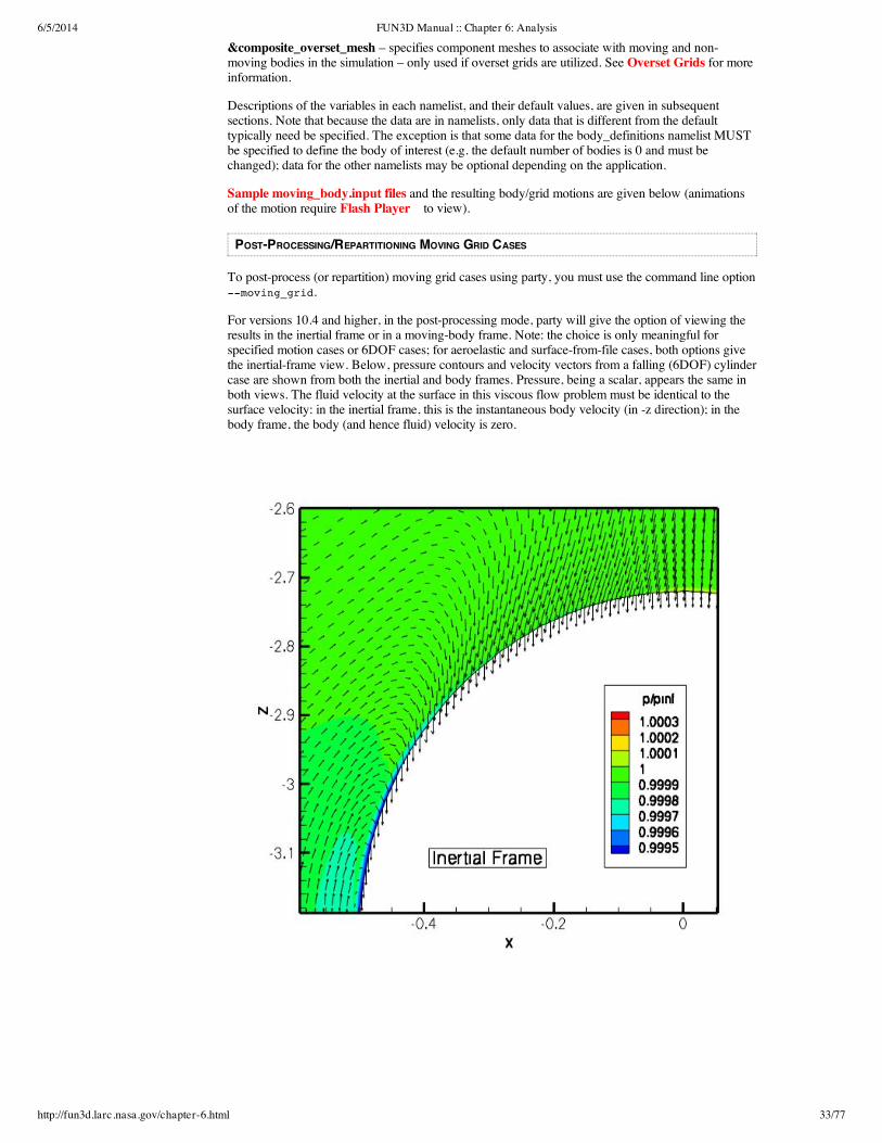
6/5/2014 FUN3D Manual :: Chapter 6: Analysis
http://fun3d.larc.nasa.gov/chapter-6.html 33/77
&composite_overset_mesh – specifies component meshes to associate with moving and non-moving bodies in the simulation – only used if overset grids are utilized. See Overset Grids for moreinformation.
Descriptions of the variables in each namelist, and their default values, are given in subsequentsections. Note that because the data are in namelists, only data that is different from the defaulttypically need be specified. The exception is that some data for the body_definitions namelist MUSTbe specified to define the body of interest (e.g. the default number of bodies is 0 and must bechanged); data for the other namelists may be optional depending on the application.
Sample moving_body.input files and the resulting body/grid motions are given below (animationsof the motion require Flash Player to view).
POST-PROCESSING/REPARTITIONING MOVING GRID CASES
To post-process (or repartition) moving grid cases using party, you must use the command line option--moving_grid.
For versions 10.4 and higher, in the post-processing mode, party will give the option of viewing theresults in the inertial frame or in a moving-body frame. Note: the choice is only meaningful forspecified motion cases or 6DOF cases; for aeroelastic and surface-from-file cases, both options givethe inertial-frame view. Below, pressure contours and velocity vectors from a falling (6DOF) cylindercase are shown from both the inertial and body frames. Pressure, being a scalar, appears the same inboth views. The fluid velocity at the surface in this viscous flow problem must be identical to thesurface velocity: in the inertial frame, this is the instantaneous body velocity (in -z direction); in thebody frame, the body (and hence fluid) velocity is zero.

6/5/2014 FUN3D Manual :: Chapter 6: Analysis
http://fun3d.larc.nasa.gov/chapter-6.html 34/77
DEFINING MOVING BODIES
The following namelist, which is input via the moving_body.input file, is used to specify one ormore bodies as collections of boundary surfaces within the mesh. This namelist is required for allmoving body/mesh cases, i.e. whenever the --moving_grid command line option is invoked. Theinput structure is fairly general in that the motion of multiple bodies may be specified, andconnections between various bodies may be specified via family trees. For example, a wing-flapsystem may be defined such that the flap is a child of the wing. Thus the flap inherits any motionspecified for the wing, and may have its’ own motion specified on top of that. For example, the wingmay be specified to translate up and down, and the flap to rotate about a hinge line such that the netmotion of the flap is a combination of translation and rotation. Such a wing-flap system is given inone of the examples below.
A (G) following a variable description means that this is a global descriptor, i.e. applicable to allmoving bodies; a (B) following a variable description means that the data may be specified for eachmoving body
&body_definitions namelist
n_moving_bodies Number of bodies in motion (G) (Default: 0)body_name Name to identify the body (B) (Default: ’’)parent_name Name of the parent body (B) (Default: ’’ [indicates inertial ref. frame as
parent])n_defining_bndry Number of boundaries that define the body (B) (Default: 0)defining_bndry List of n_defining_bndry boundaries that define the body (B) (Default: 0)motion_driver Mechanism by which body motion is driven (B) (Default: ‘none’ Options:
‘forced’, ‘6dof’, ‘surface_file’, ‘motion_file’, ‘aeroelastic’)mesh_movement Type of grid movement associated with body motion (B) (Default: ‘static’
Options: ‘rigid’, ‘deform’)x_mc X-coordinate of moment center at t=0 (B) (Default: xmc from input file)y_mc Y-coordinate of moment center at t=0 (B) (Default: ymc from input file)

6/5/2014 FUN3D Manual :: Chapter 6: Analysis
http://fun3d.larc.nasa.gov/chapter-6.html 35/77
z_mc Z-coordinate of moment center at t=0 (B) (Default: zmc from input file)s_ref Reference area (non-dimensional) for force/moment normalization (B)
(Default: sref from input file)c_ref Reference length (non-dimensional) for force/moment normalization (B)
(Default: cref from input file)b_ref Reference length (non-dimensional) for force/moment normalization (B)
(Default: bref from input file)move_mc Flag to move (1) or leave the moment center fixed in space(0) (B) (Default:
1)dimensional_outputLogical flag to output the body state data (displacements, velocities, and aero
forces for each body) in dimensional form for forced or 6DOF motions (G)(Default: .false.)
body_frame_forces Logical flag to output the (aerodynamic) forces/moments on the body in thebody-frame (G) (Default: .false. i.e. output forces/moments in inertial frame)
ref_length Reference length for converting to dimensional output (G) (Default: 1.0 ft.)ref_density Reference density for converting to dimensional output (G) (Default:
0.002378 slug/ft/ft/ft)ref_velocity Reference velocity for converting to dimensional output (G) (Default: 1117.0
ft/sec)output_transform Output 4×4 transform matrix at each time step for each body (G) (Default:
.false.)
SPECIFIED BODY MOTION
The following namelist, which is input via the moving_body.input file, is used to specify how thebody is defined via the &body_definitions namelist move as a function of time. Note that this isone of several ways body motion may be specified, and is appropriate if the desired body motion maybe described as a simple rigid-body translation or rotation, with constant velocity or sinusoidally-varying displacement. For specified motions not amenable to such basic descriptions, either a 4×4transform matrix for the (rigid) body may be specified at each time step, or the (rigid or deforming)body surface points may be specified at each time step (see Body Motion via File Input), so that anydesired motion can in principle be defined (including shape-morphing bodies).
A (B) following a variable description means that the data may be specified for each moving body
&forced_motion namelist
rotate Type of rotational motion 0=none, 1=constant rotation rate, 2=sinusoidal(B) (Default: 0) For type 2, theta = rotation_amplitude x sin(2 x pi xrotation_freq x t), where t=nondimensional time
rotation_rate Rotation rate (non-dimensional) associated with rotate=1 (B) (Default:0.0)
rotation_freq Rotation reduced frequency (non-dimensional) associated with rotate=2(B) (Default: 0.0)
rotation_phase Rotation phase shift (degrees) associated with rotate=2 (B) (Default: 0.0)rotation_tphase Rotation phase shift (degrees) applied to transform matrix (B) (Default:
0.0)rotation_amplitude Rotation amplitude (degrees) associated with rotate=2 (B) (Default: 0.0)rotation_origin_x X-coordinate of rotation center (B) (Default: 0.0)rotation_origin_y Y-coordinate of rotation center (B) (Default: 0.0)rotation_origin_z Z-coordinate of rotation center (B) (Default: 0.0)rotation_vector_x X-component of unit vector along rotation axis (B) (Default: 0.0)rotation_vector_y Y-component of unit vector along rotation axis (B) (Default: 1.0)rotation_vector_z Z-component of unit vector along rotation axis (B) (Default: 0.0)rotation_start Start time (non-dimensional) of rotational motion (B) (Default: 0.0)rotation_duration Duration (non-dimensional) of rotational motion (B) (Default: 1.0e99)
translate Type of translational motion 0=none, 1=constant translation rate,2=sinusoidal (B) (Default: 0) For type 2, displacement =translation_amplitude x sin(2 x pi x translation_freq x t), wheret=nondimensional time
translation_rate Translation rate (non-dimensional) associated with translate=1 (B)(Default: 0.0)
translation_freq Translation reduced frequency (non-dimensional) associated withtranslate=2 (B) (Default: 0.0)

6/5/2014 FUN3D Manual :: Chapter 6: Analysis
http://fun3d.larc.nasa.gov/chapter-6.html 36/77
translation_phase Translation phase shift (degrees) associated with translate=2 (B) (Default:0.0)
translation_tphase Translation phase shift (degrees) applied to transform matrix (B)(Default: 0.0)
translation_amplitudeTranslation amplitude (grid units) associated with translate=2 (B)(Default: 0.0)
translation_vector_xX-component of unit vector along translation axis (B) (Default: 0.0)translation_vector_yY-component of unit vector along translation axis (B) (Default: 1.0)translation_vector_z Z-component of unit vector along translation axis (B) (Default: 0.0)translation_start Start time (non-dimensional) of translational motion (B) (Default: 0.0)
translation_durationDuration (non-dimensional) of translational motion (B) (Default: 1.0e99)
OUTPUT DATA
In version 10.4 and higher, specified body motion (&forced_motion namelist) will result in thefollowing ASCII output files being generated (below, in filenameBody_N, N is the body number):
PositionBody_N.hst Contains “CG” (rotation center) position and Euler angles (pitch,roll, yaw) as functions of time; default output is non-dimensional;Tecplot format. Note that Euler angles have multiple singularitiesand are non-unique!
VelocityBody_N.hst Contains linear and angular velocity components of the CG(rotation center) as functions of time; default output is non-dimensional; Tecplot format.
AeroForceMomentBody_N.hstContains the aerodynamic forces and moments (about the specifiedmoment center) acting on the body as functions of time; defaultoutput is non-dimensional; Tecplot format.
TransformMatrixBody_N.hst(Optional) Contains the 4×4 transform matrix for the body as afunction of time; format is described in the file header. Output onlyif output_transform = .true. in namelist &body_definitions.A similar file, TransformMatrixObserver.hst (for the motion ofthe observer frame ) is also output if output_transform = .true.
Note: these files are created from scratch if irest=0 or irest=-1; any existing files with these namesare overwritten. The files are appended to (if they exist) when restarting with irest=1. If they havebeen deleted before restarting with irest=1 they will be created but the preceding history will belost.
In addition to the above files, the [project]_hist.dat file contains the x, y, and z components of thespecified rotation vector, as well as the position of the rotation origin as functions of time. Except forspecial cases, the rotation vector components will differ from the Euler angles. Note that the data inthis file is for body 1 only, and is also output from versions prior to 10.4.
SPECIFIED OBSERVER MOTION (FOR ANIMATION)
The following namelist, which is input via the moving_body.input file, is used to specify the motionof an observer. This optional namelist is only used when requesting Flow Visualization OutputDirectly From Flow Solver for cases that involve moving bodies, and is not available in versionsprior to 10.4. If the observer_motion is specified, then the resulting animation will be from theobserver’s reference frame rather than the (default) inertial reference frame. This capability may beused for, among other things, assessing relative motions in complex dynamic motions (e.g. insuringthat the cyclic pitch in a rotor simulation is correctly enforced). The data to specify observer motion isanalogous to specifying body motion; the observer motion is applied on a global basis (G).
&observer_motion namelist
ob_parent_name Parent reference frame for observer (G) (Default: ’’ [indicates inertialref. frame]
ob_rotate Type of rotational motion 0=none, 1=constant rotation rate,2=sinusoidal (G) (Default: 0)
ob_rotation_rate Rotation rate (non-dimensional) associated with rotate=1 (G)(Default: 0.0)
ob_rotation_freq Rotation reduced frequency (non-dimensional) associated withrotate=2 (G) (Default: 0.0)
ob_rotation_phase Rotation phase shift (degrees) associated with rotate=2 (G) (Default:
6/5/2014 FUN3D Manual :: Chapter 6: Analysis
http://fun3d.larc.nasa.gov/chapter-6.html 37/77
0.0)ob_rotation_tphase Rotation phase shift (degrees) applied to transform matrix (G)
(Default: 0.0)ob_rotation_amplitude Rotation amplitude (degrees) associated with rotate=2 (G) (Default:
0.0)ob_rotation_origin_x X-coordinate of rotation center (G) (Default: 0.0)ob_rotation_origin_y Y-coordinate of rotation center (G) (Default: 0.0)ob_rotation_origin_z Z-coordinate of rotation center (G) (Default: 0.0)ob_rotation_vector_x X-component of unit vector along rotation axis (G) (Default: 0.0)ob_rotation_vector_y Y-component of unit vector along rotation axis (G) (Default: 1.0)ob_rotation_vector_z Z-component of unit vector along rotation axis (G) (Default: 0.0)
ob_translate Type of translational motion 0=none, 1=constant translation rate,2=sinusoidal (G) (Default: 0)
ob_translation_rate Translation rate (non-dimensional) associated with translate=1 (G)(Default: 0.0)
ob_translation_freq Translation reduced frequency (non-dimensional) associated withtranslate=2 (G) (Default: 0.0)
ob_translation_phase Translation phase shift (degrees) associated with translate=2 (G)(Default: 0.0)
ob_translation_tphase Translation phase shift (degrees) applied to transform matrix (G)(Default: 0.0)
ob_translation_amplitudeTranslation amplitude (grid units) associated with translate=2 (G)(Default: 0.0)
ob_translation_vector_xX-component of unit vector along translation axis (G) (Default: 0.0)ob_translation_vector_yY-component of unit vector along translation axis (G) (Default: 1.0)ob_translation_vector_z Z-component of unit vector along translation axis (G) (Default: 0.0)
If it is desired to have the observer in the frame of a moving body whose motion is specified, orresults from 6DOF motion, then all that is needed is to set ob_parent_name equal to the name of thatbody (in quotes), without any further &observer_motion data. There may be cases in which there isno body with the desired motion, in which case the &observer_motion parameters above can beused to specify the motion relative to the ob_parent_name reference system. Note: a body whosemotion is specified via file input, or whose motion is the result of aeroelastic motion, cannot be usedas the ob_parent_name.

6/5/2014 FUN3D Manual :: Chapter 6: Analysis
http://fun3d.larc.nasa.gov/chapter-6.html 38/77
BODY MOTION VIA FILE INPUT
There are currently two ways to specify arbitrary body/grid motion via user-supplied files to describethe motion. The first is applicable to rigid-body motion with either rigid or deforming meshes. Thesecond is applicable to either rigid or deforming bodies but must be used in conjunction with thedeforming mesh motion.
1) Specifying the 4×4 Transform Matrix as a Function of Time – Rigid Body / Rigid or Deforming Grid
To utilize this option, you must set motion_driver = 'motion_file' in the &body_definitionsnamelist. In addition, at least some data in the &motion_from_file namelist must be specified:
&motion_from_file namelist
n_time_slices_fileNumber of time steps at which the transform matrix will be supplied (B)(Default: 0)
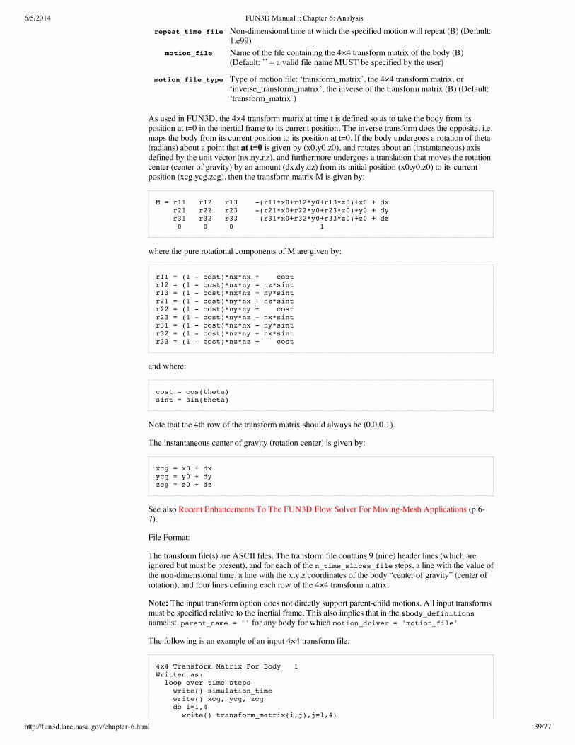
6/5/2014 FUN3D Manual :: Chapter 6: Analysis
http://fun3d.larc.nasa.gov/chapter-6.html 39/77
repeat_time_file Non-dimensional time at which the specified motion will repeat (B) (Default:1.e99)
motion_file Name of the file containing the 4×4 transform matrix of the body (B)(Default: ’’ – a valid file name MUST be specified by the user)
motion_file_type Type of motion file: ‘transform_matrix’, the 4×4 transform matrix, or‘inverse_transform_matrix’, the inverse of the transform matrix (B) (Default:‘transform_matrix’)
As used in FUN3D, the 4×4 transform matrix at time t is defined so as to take the body from itsposition at t=0 in the inertial frame to its current position. The inverse transform does the opposite, i.e.maps the body from its current position to its position at t=0. If the body undergoes a rotation of theta(radians) about a point that at t=0 is given by (x0,y0,z0), and rotates about an (instantaneous) axisdefined by the unit vector (nx,ny,nz), and furthermore undergoes a translation that moves the rotationcenter (center of gravity) by an amount (dx,dy,dz) from its initial position (x0,y0,z0) to its currentposition (xcg,ycg,zcg), then the transform matrix M is given by:
M = r11 r12 r13 -(r11*x0+r12*y0+r13*z0)+x0 + dx r21 r22 r23 -(r21*x0+r22*y0+r23*z0)+y0 + dy r31 r32 r33 -(r31*x0+r32*y0+r33*z0)+z0 + dz 0 0 0 1
where the pure rotational components of M are given by:
r11 = (1 - cost)*nx*nx + costr12 = (1 - cost)*nx*ny - nz*sintr13 = (1 - cost)*nx*nz + ny*sintr21 = (1 - cost)*ny*nx + nz*sintr22 = (1 - cost)*ny*ny + costr23 = (1 - cost)*ny*nz - nx*sintr31 = (1 - cost)*nz*nx - ny*sintr32 = (1 - cost)*nz*ny + nx*sintr33 = (1 - cost)*nz*nz + cost
and where:
cost = cos(theta)sint = sin(theta)
Note that the 4th row of the transform matrix should always be (0,0,0,1).
The instantaneous center of gravity (rotation center) is given by:
xcg = x0 + dxycg = y0 + dyzcg = z0 + dz
See also Recent Enhancements To The FUN3D Flow Solver For Moving-Mesh Applications (p 6-7).
File Format:
The transform file(s) are ASCII files. The transform file contains 9 (nine) header lines (which areignored but must be present), and for each of the n_time_slices_file steps, a line with the value ofthe non-dimensional time, a line with the x,y,z coordinates of the body “center of gravity” (center ofrotation), and four lines defining each row of the 4×4 transform matrix.
Note: The input transform option does not directly support parent-child motions. All input transformsmust be specified relative to the inertial frame. This also implies that in the &body_definitionsnamelist, parent_name = '' for any body for which motion_driver = 'motion_file'
The following is an example of an input 4×4 transform file:
4x4 Transform Matrix For Body 1Written as: loop over time steps write() simulation_time write() xcg, ycg, zcg do i=1,4 write() transform_matrix(i,j),j=1,4)

6/5/2014 FUN3D Manual :: Chapter 6: Analysis
http://fun3d.larc.nasa.gov/chapter-6.html 40/77
end do end time step loop 0.0000000000E+00 0.2500000000E+00 0.0000000000E+00 0.0000000000E+00 0.1000000000E+01 0.0000000000E+00 0.0000000000E+00 0.0000000000E+00 0.0000000000E+00 0.1000000000E+01 0.0000000000E+00 0.0000000000E+00 0.0000000000E+00 0.0000000000E+00 0.1000000000E+01 0.0000000000E+00 0.0000000000E+00 0.0000000000E+00 0.0000000000E+00 0.1000000000E+01 0.3228110000E+00 0.2500000000E+00 0.0000000000E+00 0.0000000000E+00 0.9999968340E+00 0.0000000000E+00 0.2516342349E-02 0.7914986049E-06 0.0000000000E+00 0.1000000000E+01 0.0000000000E+00 0.0000000000E+00 -0.2516342349E-02 0.0000000000E+00 0.9999968340E+00 0.6290855872E-03 0.0000000000E+00 0.0000000000E+00 0.0000000000E+00 0.1000000000E+01 0.6456220000E+00 0.2500000000E+00 0.0000000000E+00 0.0000000000E+00 0.9999873485E+00 0.0000000000E+00 0.5030185447E-02 0.3162865712E-05 0.0000000000E+00 0.1000000000E+01 0.0000000000E+00 0.0000000000E+00 -0.5030185447E-02 0.0000000000E+00 0.9999873485E+00 0.1257546362E-02 0.0000000000E+00 0.0000000000E+00 0.0000000000E+00 0.1000000000E+01
etc.
The file format is the same regardless of whether motion_file_type is ‘transform_matrix’ or‘inverse_transform_matrix’
It may be noted that this file format is identical to that generated when output_transform =.true. in the &body_definitions namelist. So, if the motion_file_type is ‘transform_matrix’and the file contains the transform at times corresponding exactly to each time step in the simulation,the output transform file can be compared (to machine precision) against the input transform file toverify that the input data has been read correctly.
As implied above, the time increments in the motion_file need not correspond to the time stepspecified in the fun3d.nml file; however, it is recommended that this be the case. If the timeincrements in the motion_file do not correspond to the time step specified in the fun3d.nml file,the specified transforms are “interpolated” to the time dictated by the time step. Interpolated is quotedbecause in fact transform matrices cannot be directly interpolated. Rather, the transforms are firstconverted into quaternions, the quaternions (and centers of gravity/rotation) are linearly interpolatedand then recast as the required transform matrix. This interpolation process has not been widely testedat this point in time.
2) Specifying the Body as a Function of Time – Rigid or Deforming Body / Deforming Grid
NOTE: this option requires that Mesh Deformation be used for grid movement.
If the &surface_motion_from_file namelist is specified in the moving_body.input file, i then thesolver will attempt to read in the specified number of files for the body:
&surface_motion_from_file namelist
n_time_slicesNumber of files defining motion of the body (B) (Default: 0)repeat_time Non-dimensional time at which motion in files will repeat (B) (Default: 1.e99)
The names of the file(s) containing the surface data as a function of time MUST adhere to the namingconvention given below. The points defining the surface(s) in the file(s) must correspond to thesurface(s) defined in the &body_definitions namelist. Generally speaking, the time span coveredby these files should either encompass the time span of the current run, or the period of motion if thebody motion is cyclic. The exception to this is for static aeroelastic cases, where the flow solver isonly periodically coupled to a structural solver; in this case only one surface file is read in (for anyone body) at the start of a run, and the TIME data is ignored (and in fact is not required).
The time values given in the files need not correspond to increments of time as specified by theparameter time_step_nondim in fun3d.nml (DT in the ginput.faces in release 10.4.1 and before)(though it is probably best to do so). For example, if DT=1.0, then as the code executes, the non-dimensional time runs as 0.0, 1.0, 2.0, 3.0… The times specified at the top of the surface files (seebelow) might be 0.0, 2.5, 5.0, 7.5… In this case the positions defined in the files are linearlyinterpolated in time to the current solver time.
Surface File Naming Convention:
{project}.bodyN_timestepM
where:
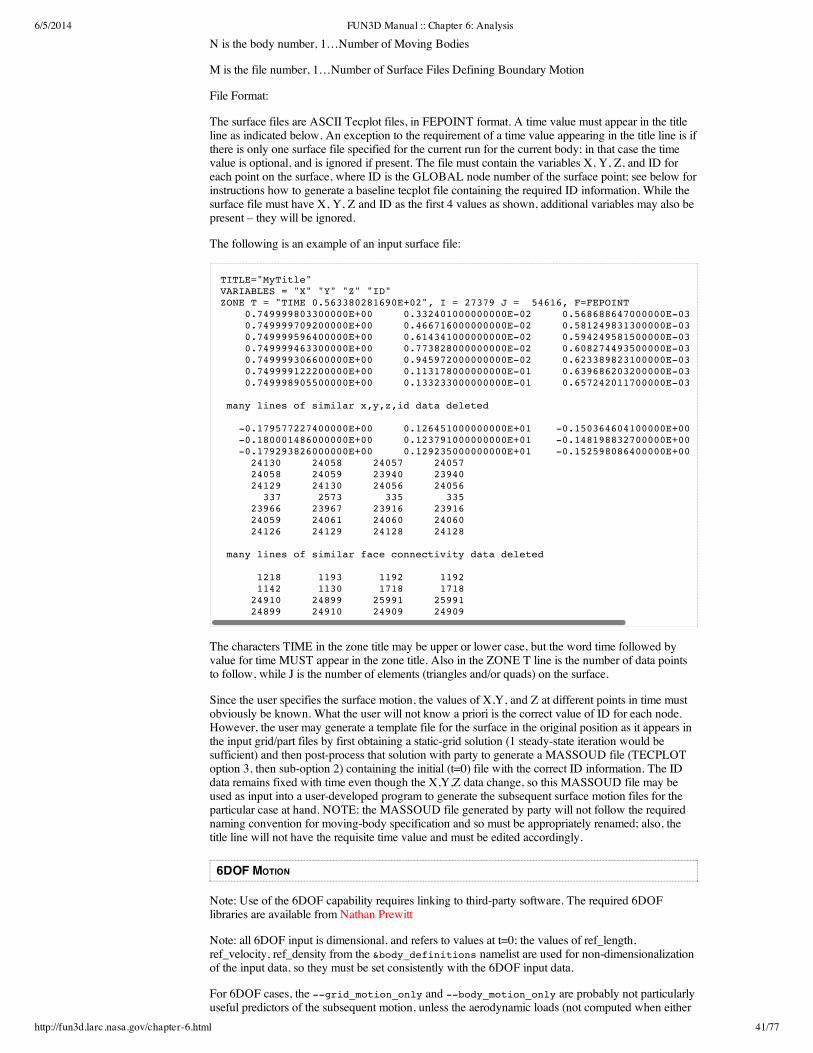
6/5/2014 FUN3D Manual :: Chapter 6: Analysis
http://fun3d.larc.nasa.gov/chapter-6.html 41/77
N is the body number, 1…Number of Moving Bodies
M is the file number, 1…Number of Surface Files Defining Boundary Motion
File Format:
The surface files are ASCII Tecplot files, in FEPOINT format. A time value must appear in the titleline as indicated below. An exception to the requirement of a time value appearing in the title line is ifthere is only one surface file specified for the current run for the current body; in that case the timevalue is optional, and is ignored if present. The file must contain the variables X, Y, Z, and ID foreach point on the surface, where ID is the GLOBAL node number of the surface point; see below forinstructions how to generate a baseline tecplot file containing the required ID information. While thesurface file must have X, Y, Z and ID as the first 4 values as shown, additional variables may also bepresent – they will be ignored.
The following is an example of an input surface file:
The characters TIME in the zone title may be upper or lower case, but the word time followed byvalue for time MUST appear in the zone title. Also in the ZONE T line is the number of data pointsto follow, while J is the number of elements (triangles and/or quads) on the surface.
Since the user specifies the surface motion, the values of X,Y, and Z at different points in time mustobviously be known. What the user will not know a priori is the correct value of ID for each node.However, the user may generate a template file for the surface in the original position as it appears inthe input grid/part files by first obtaining a static-grid solution (1 steady-state iteration would besufficient) and then post-process that solution with party to generate a MASSOUD file (TECPLOToption 3, then sub-option 2) containing the initial (t=0) file with the correct ID information. The IDdata remains fixed with time even though the X,Y,Z data change, so this MASSOUD file may beused as input into a user-developed program to generate the subsequent surface motion files for theparticular case at hand. NOTE: the MASSOUD file generated by party will not follow the requirednaming convention for moving-body specification and so must be appropriately renamed; also, thetitle line will not have the requisite time value and must be edited accordingly.
6DOF MOTION
Note: Use of the 6DOF capability requires linking to third-party software. The required 6DOFlibraries are available from Nathan Prewitt
Note: all 6DOF input is dimensional, and refers to values at t=0; the values of ref_length,ref_velocity, ref_density from the &body_definitions namelist are used for non-dimensionalizationof the input data, so they must be set consistently with the 6DOF input data.
For 6DOF cases, the --grid_motion_only and --body_motion_only are probably not particularlyuseful predictors of the subsequent motion, unless the aerodynamic loads (not computed when either
TITLE="MyTitle" VARIABLES = "X" "Y" "Z" "ID" ZONE T = "TIME 0.563380281690E+02", I = 27379 J = 54616, F=FEPOINT 0.749999803300000E+00 0.332401000000000E-02 0.568688647000000E-03 756948 0.749999709200000E+00 0.466716000000000E-02 0.581249831300000E-03 756949 0.749999596400000E+00 0.614341000000000E-02 0.594249581500000E-03 756950 0.749999463300000E+00 0.773828000000000E-02 0.608274493500000E-03 756951 0.749999306600000E+00 0.945972000000000E-02 0.623389823100000E-03 756952 0.749999122200000E+00 0.113178000000000E-01 0.639686203200000E-03 756953 0.749998905500000E+00 0.133233000000000E-01 0.657242011700000E-03 756955
many lines of similar x,y,z,id data deleted
-0.179577227400000E+00 0.126451000000000E+01 -0.150364604100000E+00 872982 -0.180001486000000E+00 0.123791000000000E+01 -0.148198832700000E+00 872983 -0.179293826000000E+00 0.129235000000000E+01 -0.152598086400000E+00 872984 24130 24058 24057 24057 24058 24059 23940 23940 24129 24130 24056 24056 337 2573 335 335 23966 23967 23916 23916 24059 24061 24060 24060 24126 24129 24128 24128
many lines of similar face connectivity data deleted
1218 1193 1192 1192 1142 1130 1718 1718 24910 24899 25991 25991 24899 24910 24909 24909

6/5/2014 FUN3D Manual :: Chapter 6: Analysis
http://fun3d.larc.nasa.gov/chapter-6.html 42/77
option is invoked) have very little impact on the dynamics.
A (B) after the description indicates the data may be specified for each body; (1-3,B) indicates one orall of 3 (x,y,z) components may be specified for each body. For example body_lin_vel(2,3) would beinput to specify an initial y-component of velocity for body 3.
&sixdof_motion namelist
mass Mass of the body (B) (Default: 1.0)cg_x X-coordinate of CG (B) (Default: 0.0)cg_y Y-coordinate of CG (B) (Default: 0.0)cg_z Z-coordinate of CG (B) (Default: 0.0)i_xx Moment of inertia about x axis (B) (Default: 1.0)i_yy Moment of inertia about y axis (B) (Default: 1.0)i_xx Moment of inertia about z axis (B) (Default: 1.0)i_xy Moment of inertia about x-y axis (B) (Default: 0.0)i_xz Moment of inertia about x-z axis (B) (Default: 0.0)i_yz Moment of inertia about y-z axis (B) (Default: 0.0)
body_lin_vel Components of linear velocity (1-3,B) (Default: 0.0, 0.0, 0.0)body_ang_vel Components of angular velocity (1-3,B) (Default: 0.0, 0.0, 0.0)euler_ang Euler angles (1-3,B) (Default: 0.0, 0.0, 0.0)gravity_dir Normalized components of the gravity vector (G) (Default: 0.0, 0.0, -1.0)gravity_mag Magnitude of the gravity vector (G) (Default: 32.2)n_extforce Number of imposed external forces, excluding gravity (B) (Default: 0)n_extmoment Number of imposed external moments (B) (Default: 0)file_extforce File specifying external forces (B) (Default: ’’)file_extmomentFile specifying external moments (B) (Default: ’’)
Output Data
6DOF body motion (&sixdof_motion namelist) will result in the following output files beinggenerated (below, in filenameBody_N, N is the body number):
PositionBody_N.hst Contains CG position (as specified in &sixdof_motion) andEuler angles (pitch, roll, yaw) as functions of time; defaultoutput is non-dimensional; Tecplot format. Note that Eulerangles have multiple singularities and are non-unique!
VelocityBody_N.hst Contains linear and angular velocity components of the CG asfunctions of time; default output is non-dimensional; Tecplotformat.
AeroForceMomentBody_N.hst Contains the aerodynamic forces and moments (about the CG)acting on the body as functions of time; default output is non-dimensional; Tecplot format. Note: the aero forces andmoments in the output file are non-dimensionalized in thestandard fashion for aerodynamics; this is not the same waythey are non-dimensionalized for the 6DOF equations
ExternalForceMomentBody_N.hstContains any user-specified external forces and momentsacting on the body as functions of time; default output is non-dimensional (6DOF non-dimensionalization); Tecplot format.
Note: these files are created from scratch if irest=0 or irest=-1; any existing files with these namesare overwritten. The files are appended to (if they exist) when restarting with irest=1. If they havebeen deleted before restarting with irest=1 they will be created but the preceding history will belost.
AEROELASTIC MOTION (MODE-BASED)
NOTE: this option requires that Mesh Deformation be used for grid movement.
Note: the implementation of the modal aeroelastic analysis in FUN3D follows nearly exactly theimplementation in CFL3D, so interested parties may find some useful supplemental information onpp 191-223 of the CFL3D Tutorial.
A (G) following a variable description means that this is a global descriptor, i.e. applicable to allaeroelastic bodies; (B) means that the data may be specified for each body; (M,B) means the data may

6/5/2014 FUN3D Manual :: Chapter 6: Analysis
http://fun3d.larc.nasa.gov/chapter-6.html 43/77
be specified for each mode associated with each body. For example, freq(4,2) would specify thefrequency of mode 4 for body 2.
The modal aeroelastic capability is available in Version 10.4 and higher
&aeroelastic_modal_data namelist
nmode Number of aeroelastic modes used to represent the structural deformation (B)(Default: 0)
plot_modes Logical flag to generate tecplot files of each mode shape added to the bodysurface to help insure validity of input modal surface data (G) (Default: .false.)
single_modal_fileLogical flag to read all mode shapes from a single file for each body (G)(Default: .false. i.e. each mode in a separate file for each body)
grefl Scale factor between CFD grid units and structural dynamics equation units(B) (Default: 1.0)
uinf Free stream velocity, in structural dynamics equation units (B) (Default: 0.0)qinf Free stream dynamic pressure, in structural dynamics equation units (B)
(Default: 0.0)gdispl0 Generalized displacement of specified mode at starting time step; used to
perturb mode for excitation of dynamic response (Default: 0.0)gvel0 Generalized velocity of specified mode at starting time step; used to perturb
mode for excitation of dynamic response (Default: 0.0)gforce0 Generalized force of specified mode at starting time step; used to perturb mode
for excitation of dynamic response (Default: 0.0)gmass Generalized mass of specified mode (M,B) (Default: 0.0)freq Frequency of specified mode, rad/sec (M,B) (Default: 0.0)damp Critical damping ratio (z) of specified mode (M,B) (Default: 0.0)moddfl Type of time-varying perturbation of specified mode: 0, no perturbation; <0,
modal displacement and velocity set to 0; 1, harmonic (sinusoidal); 2,Gaussian pulse; 3, Step pulse; 5, ROM input (M,B) (Default: 0)
moddfl_amp Amplitude of perturbation of specified mode (M,B) (Default: 0.0)moddfl_freq Frequency of perturbation of specified mode if moddfl=1; half-width of
Gaussian pulse if moddfl=2 (M,B) (Default: 0.0)moddfl_t0 Time (dimensional) at which sinusoidal perturbation starts if moddfl=1; time
about which Gaussian pulse is centered if moddfl=2; start time of step pulse ifmoddfl=3 (M,B) (Default: 0.0)
moddfl_add Flag to determine whether perturbation is to be added (1) to any existing staticaeroelastic solution or whether the perturbation replaces (0) the staticaeroelastic solution (if one exists) (M,B) (Default: 0, replace)
In addition to the &aeroelastic_modal_data namelist, one or more files containing the modalsurface definitions must be provided. FUN3D accepts two types of modal files: 1) each modeassociated with an aeroelastic body is in a separate file or 2) all modes associated with an aeroelasticbody are contained in the same file. The points defining the modal surface(s) in the file(s) mustcorrespond to the surface(s) defined in the &body_definitions namelist.
In addition, for ROM (Reduced Order Model) analysis (triggered by moddfl=5), an additional file,called rom_inputs_bodyN.dat (N the body number), must be available. Rather than give an exampleof a rom_inputs_bodyN.dat file, the following code snippet shows how the file is read:
! read number of time steps and starting time step from the rom data file read(iu,*) ncyc_rom, nstart_rom
! read number of modes in the rom data file read(iu,*) nmodes_rom_file
! read the list of modes to (potentially) be used for rom read(iu,*) (rom_data(body)%rom_mode(nm), nm=1,nmodes_rom_file)
! read the rom excitation data (modal displacement and velocity) do timestep = 1,ncyc_rom do nm=1,nmodes_rom_file nm1 = rom_data(body)%rom_mode(nm) read(iu,*,iostat=istop) rom_data(body)%gen_disp(nm1,timestep), & rom_data(body)%gen_vel(nm1,timestep) end do end do

6/5/2014 FUN3D Manual :: Chapter 6: Analysis
http://fun3d.larc.nasa.gov/chapter-6.html 44/77
where ncyc_rom is the number of timesteps contained in the file, and nstart_rom is the timestep atwhich to start the ROM excitation for the current run. Thus nstart_rom should be 1 for the first run,and if all time steps are not completed in a single run, then nstart_rom should be set tolast_time_step_of_previous_run + 1 for the next run. Any modes with moddfl=5 in themoving_body.input file must appear in the rom_inputs_bodyN.dat file (in both the rom_mode list andthe excitation data).
Modal Surface File Naming Convention:
1) Separate file for each mode:
{project}.bodyN_modeM
2) All modes in one file:
{project}.bodyN_all_modes
where:
N is the body number
M is the mode number
File Format:
The modal surface files are ASCII Tecplot files, in FEPOINT format. The file must contain thevariables X, Y, Z and ID as the first four variables, where X, Y, Z define the baseline surface and IDis the GLOBAL node number. For the single-mode-per-file format, these are followed by the modalcoordinates XMD, YMD, ZMD; for the all-modes-in-one-file format, XMD1, YMD1, ZMD1,XMD2, YMD2, ZMD2, etc, follow.
The following is an example of a modal surface file (containing a single mode):
The starting point for generating a modal shape file as shown above is to first obtain a static-gridsolution (1 steady state iteration would be sufficient) and then post-process that solution with party togenerate a MASSOUD file (TECPLOT option 3, then sub-option 2) containing the baseline file withthe correct X, Y, Z and ID information. This baseline file can then be used as input into a user-developed program to add the appropriate XMD, YMD, ZMD data for the case at hand (theX,Y,Z,ID data remain unchanged). NOTE: the MASSOUD file generated by party will not followthe required naming convention for modal file specification and so must be appropriately renamed.
Output Data
Aeroelastic body motion (&aeroelastic_modal_data namelist) will result in the following outputfiles being generated (below, in filename_bodyN_modeM, N is the body number and M is the mode
title="Mode 1" variables = "x" "y" "z" "id" "xmd" "ymd" "zmd" zone t = mode1, i = 176, j = 88,f=fepoint 0.160000000000E+02 0.000000000000E+00 0.000000000000E+00 9377 0.000000000000E+00 0.000000000000E+00 0.408356833737E+00 0.160000000000E+02 -0.640000000000E+02 0.000000000000E+00 9442 0.000000000000E+00 0.000000000000E+00 0.408356833737E+00 0.158624877930E+02 0.000000000000E+00 -0.195790082224E-01 9571 0.000000000000E+00 0.000000000000E+00 0.408374846989E+00 0.158624877930E+02 0.000000000000E+00 0.195790082224E-01 9572 0.000000000000E+00 0.000000000000E+00 0.408374846989E+00 0.158624877930E+02 -0.640000000000E+02 -0.195790082224E-01 9639 0.000000000000E+00 0.000000000000E+00 0.408374846989E+00 0.158624877930E+02 -0.640000000000E+02 0.195790082224E-01 9640 0.000000000000E+00 0.000000000000E+00 0.408374846989E+00 0.156976051331E+02 0.000000000000E+00 -0.427785292272E-01 9769 0.000000000000E+00 0.000000000000E+00 0.408396445602E+00
many lines of similar x,y,z,id,xmd,ymd,zmd data deleted
0.368598237408E-03 -0.640000000000E+02 0.139784077182E-01 19630 0.000000000000E+00 0.000000000000E+00 0.410452686861E+00 0.000000000000E+00 0.000000000000E+00 0.000000000000E+00 19759 0.000000000000E+00 0.000000000000E+00 0.410452735145E+00 0.000000000000E+00 -0.640000000000E+02 0.000000000000E+00 19824 0.000000000000E+00 0.000000000000E+00 0.410452735145E+00 1 2 5 3 3 5 9 7 7 9 13 11 11 13 17 15 15 17 21 19 19 21 25 23 23 25 29 27
many lines of similar face connectivity data deleted
16 18 14 12 12 14 10 8 8 10 6 4 4 6 2 1

6/5/2014 FUN3D Manual :: Chapter 6: Analysis
http://fun3d.larc.nasa.gov/chapter-6.html 45/77
number):
aehist_bodyN_modeM.datContains the generalized displacement, generalized velocity, andgeneralized force for mode M of body N as functions of time; the outputis non-dimensional;. Tecplot format.
In addition, if the plot_modes variable is set to .true. in the &aeroelastic_modal_data namelist,then the following files are also output:
aesurf_bodyN_modeM.datContains the x, y, z coordinates of a surface created by adding thebaseline (rigid) shape of body N to the input modal shape of mode M,read from the {project}.bodyN_modeM or {project}.bodyN_all_modesfiles. As such it is a tool for assessing if the modal shapes have beenspecified and read correctly. Tecplot format.
SAMPLE MOVING_BODY.INPUT FILES
The first example constitutes a simple pitching airfoil, in which the mesh surrounding the airfoilmoves rigidly with the airfoil. This example illustrates a shortcut: to indicate a body is made up of allsolid surfaces in the mesh, without having to list each boundary surface, set n_defining_bndry = -1,and then use any integer number (0 is fine) for defining_bndry. Note that this shortcut is onlyapplicable for n_moving_bodies = 1:
(Animation requires Flash Player‘g to view)
&body_definitions n_moving_bodies = 1, ! number of bodies in motion body_name(1) = 'airfoil', ! name must be in quotes parent_name(1) = '', ! '' means motion relative to inertial ref frame

6/5/2014 FUN3D Manual :: Chapter 6: Analysis
http://fun3d.larc.nasa.gov/chapter-6.html 46/77
The second example is for a wing with a flap. The wing (‘main’) is constituted from boundary 1 inthe mesh, while the flap (‘flap’) is constituted from boundary 2 in the mesh. The wing undergoes aplunging motion in the z-direction, while the flap undergoes a pitching motion about an axis parallelto its’ leading edge. The flap is identified as a child of the wing, so that the complete motion of theflap consists of the inherited wing plunging motion plus the flap pitching motion. This 2-body motioncannot be accommodated with rigid mesh motion (unless overset, not considered here), somesh_movement is chosen as ‘deform’:
(Animation requires Flash Player‘g to view)
n_defining_bndry(1) = -1, ! shortcut to specify all solid surfaces defining_bndry(1,1) = 0, ! index 1: boundary number 2: body number; use any number for shortcut motion_driver(1) = 'forced', ! 'forced', '6dof', 'surface_file', 'motion_file', 'aeroelastic' mesh_movement(1) = 'rigid', ! 'rigid', 'deform' x_mc(1) = 0.25, ! x-coordinate of moment_center y_mc(1) = 0.0, ! y-coordinate of moment_center z_mc(1) = 0.0, ! z-coordinate of moment_center move_mc(1) = 1 ! move mom. cntr with body/grid: 0=no, 1=yes/&forced_motion rotate(1) = 2, ! rotation type: 1=constant rate 2=sinusoidal rotation_rate(1) = 0.0, ! rate of rotation rotation_freq(1) = 0.015489, ! reduced rotation frequency rotation_amplitude(1) = 4.59, ! max rotational displacement rotation_origin_x(1) = 0.25, ! x-coordinate of rotation origin rotation_origin_y(1) = 0.0, ! y-coordinate of rotation origin rotation_origin_z(1) = 0.0, ! z-coordinate of rotation origin rotation_vector_x(1) = 0.0, ! unit vector x-component along rotation axis rotation_vector_y(1) = 1.0, ! unit vector y-component along rotation axis rotation_vector_z(1) = 0.0, ! unit vector z-component along rotation axis/
&body_definitions n_moving_bodies = 2, ! number of bodies in motion body_name(1) = 'main', ! name must be in quotes body_name(2) = 'flap', ! name must be in quotes parent_name(1) = '', ! '' means motion relative to inertial ref frame parent_name(2) = 'main', ! '' means motion relative to inertial ref frame n_defining_bndry(1) = 1, ! number of boundaries that define this body n_defining_bndry(2) = 1, ! number of boundaries that define this body defining_bndry(1,1) = 1, ! index 1: boundary number index 2: body number defining_bndry(1,2) = 2, ! index 1: boundary number index 2: body number motion_driver(1) = 'forced', ! 'forced', '6dof', 'surface_file', 'motion_file', 'aeroelastic' motion_driver(2) = 'forced', ! 'forced', '6dof', surface_file', 'motion_file', 'aeroelastic' mesh_movement(1) = 'deform', ! 'rigid', 'deform'
6/5/2014 FUN3D Manual :: Chapter 6: Analysis
http://fun3d.larc.nasa.gov/chapter-6.html 47/77
The next example consists of a grid with two solid boundaries (boundaries number 2 and 3 in themapbc file) representing two blades of a rotor. These two surfaces are grouped for the purpose ofmotion specification into 5 moving “bodies”: 1) ‘hub’ contains both blades and the surrounding meshundergoes rigid mesh rotation at the angular speed of the rotor system; 2) ‘flap1’ is the first blade, andthe surrounding mesh undergoes mesh deformation to accommodate a sinusoidal flapping motionabout the blade root; 3) ‘blade1’ is used to specify a sinusoidal pitching motion about a spanwise axisof the first blade; 4) ‘flap2’ and; 5) ‘blade2’ specify the corresponding motions of the second blade.Thus the complete 5-body system defines a 2-bladed rotor undergoing a general rotation about acommon axis, with simultaneous flapping and pitching of each blade. The rotation, flap, and pitchaxes are all distinct. Each blade undergoes one flap and one pitch cycle for every rotation of thecomplete system. The flap and pitch amplitudes are both +/- 10 degrees.
(Animation requires Flash Player‘g to view)
mesh_movement(2) = 'deform', ! 'rigid', 'deform' x_mc(1) = 0.25, ! x-coordinate of moment_center x_mc(2) = 0.25, ! x-coordinate of moment_center y_mc(1) = 0.0, ! y-coordinate of moment_center y_mc(2) = 0.0, ! y-coordinate of moment_center z_mc(1) = 0.0, ! z-coordinate of moment_center z_mc(2) = 0.0, ! z-coordinate of moment_center move_mc(1) = 0, ! do not move mom. cntr with body/grid move_mc(2) = 0 ! do not move mom. cntr with body/grid/
&forced_motion translate(1) = 2, ! translation type: 1=constant rate 2=sinusoidal rotate(2) = 2, ! rotation type: 1=constant rate 2=sinusoidal translation_freq(1) = 0.03, ! reduced translation frequency rotation_freq(2) = 0.06, ! reduced rotation frequency translation_amplitude(1) = -0.1, ! max translational displacement rotation_amplitude(2) = +5.00, ! max rotational displacement rotation_origin_x(2) = 0.7798, ! x-coordinate of rotation origin rotation_origin_y(2) = 0.0, ! y-coordinate of rotation origin rotation_origin_z(2) = 0.0, ! z-coordinate of rotation origin translation_vector_x(1) = 0.0, ! unit vector x-component along translation axis rotation_vector_x(2) = 0.0885398,! unit vector x-component along rotation axis translation_vector_y(1) = 0.0, ! unit vector y-component along translation axis rotation_vector_y(2) = 0.996073, ! unit vector y-component along rotation axis translation_vector_z(1) = 1.0, ! unit vector z-component along translation axis rotation_vector_z(2) = 0.0, ! unit vector z-component along rotation axis/

6/5/2014 FUN3D Manual :: Chapter 6: Analysis
http://fun3d.larc.nasa.gov/chapter-6.html 48/77
&body_definitions n_moving_bodies = 5, ! number of bodies in motion body_name(1) = 'hub', ! name must be in quotes body_name(2) = 'flap1' body_name(3) = 'blade1', body_name(4) = 'flap2' body_name(5) = 'blade2', parent_name(1) = '', ! '' means motion relative to inertial ref frame parent_name(2) = 'hub' parent_name(3) = 'flap1', parent_name(4) = 'hub' parent_name(5) = 'flap2', n_defining_bndry(1) = 2, ! number of boundaries that define this body n_defining_bndry(2) = 1, n_defining_bndry(3) = 1, n_defining_bndry(4) = 1, n_defining_bndry(5) = 1, defining_bndry(1,1) = 2, ! index 1: boundary number index 2: body number defining_bndry(2,1) = 3, defining_bndry(1,2) = 2, defining_bndry(1,3) = 2, defining_bndry(1,4) = 3, defining_bndry(1,5) = 3, motion_driver(1) = 'forced', ! options: 'forced', '6dof', 'surface_file', 'motion_file', 'aeroelastic' motion_driver(2) = 'forced', motion_driver(3) = 'forced', motion_driver(4) = 'forced', motion_driver(5) = 'forced', mesh_movement(1) = 'rigid', ! options: 'rigid', 'deform' mesh_movement(2) = 'deform', mesh_movement(3) = 'deform', mesh_movement(4) = 'deform', mesh_movement(5) = 'deform',/
&forced_motion rotate(1) = 1, ! rotation type: 1=constant rate 2=sinusoidal rotate(2) = 2, rotate(3) = 2, rotate(4) = 2, rotate(5) = 2, rotation_rate(1) = -0.011712921516, rotation_freq(2) = 0.00186416935695, ! reduced rotation frequency rotation_freq(3) = 0.00186416935695, rotation_freq(4) = 0.00186416935695, rotation_freq(5) = 0.00186416935695, rotation_amplitude(2) = +10.00, ! flap blade 1 rotation_amplitude(3) = +10.00, ! pitch blade 1 rotation_amplitude(4) = +10.00, ! flap blade 2 rotation_amplitude(5) = +10.00, ! pitch blade 2 rotation_origin_x(1) = 0.0, ! x-coordinate of rotation origin rotation_origin_y(1) = 0.0, ! y-coordinate of rotation origin rotation_origin_z(1) = 0.0, ! z-coordinate of rotation origin rotation_origin_x(2) = -1.875, rotation_origin_y(2) = +6.75, rotation_origin_z(2) = 0.0589, rotation_origin_x(3) = -1.875, rotation_origin_y(3) = +6.75, rotation_origin_z(3) = 0.0589, rotation_origin_x(4) = +1.875, rotation_origin_y(4) = -6.75, rotation_origin_z(4) = 0.0589, rotation_origin_x(5) = +1.875, rotation_origin_y(5) = -6.75, rotation_origin_z(5) = 0.0589, rotation_vector_x(1) = 0.0, ! unit vector x-component along rotation axis rotation_vector_y(1) = 0.0, ! unit vector y-component along rotation axis rotation_vector_z(1) = 1.0, ! unit vector z-component along rotation axis rotation_vector_x(2) = 1.0, rotation_vector_y(2) = 0.0, rotation_vector_z(2) = 0.0, rotation_vector_x(3) = 0.0, rotation_vector_y(3) = 1.0, rotation_vector_z(3) = 0.0, rotation_vector_x(4) = -1.0, rotation_vector_y(4) = 0.0, rotation_vector_z(4) = 0.0, rotation_vector_x(5) = 0.0,
6/5/2014 FUN3D Manual :: Chapter 6: Analysis
http://fun3d.larc.nasa.gov/chapter-6.html 49/77
The next example consists of a wing (comprised of boundaries 7-16 in the mapbc file) in which thesurface motion is specified via a series of 73 files, each representing an instant of (non-dimensional)time between t=0 and t=1. The surface motion given by the files is repeated after the repeat_time of1.0. Details describing the format for the surface motion files, as well as an example of such a filemay be found in the section Body Motion via File Input
MESH DEFORMATION
Mesh deformation is invoked from within the flow solver (as opposed to the stand-alone meshdeformation code used in the design process) when running in time accurate node (itime > 0) with thecommandline option --moving_grid and the mesh_movement variable for one or more bodiesdefined in the moving_body.input file is set to 'deform'. Mesh deformation is also invoked fromwithin the flow solver if running in steady-state mode (itime=0) and the commandline option --
rotation_vector_y(5) = 1.0, rotation_vector_z(5) = 0.0,/
&body_definitions n_moving_bodies = 1, ! number of bodies in motion body_name(1) = 'wing', ! name must be in quotes parent_name(1) = '', ! '' means motion relative to inertial ref frame n_defining_bndry(1) = 10, ! number of boundaries that define this body defining_bndry(1,1) = 7, ! index 1: boundary number index 2: body number defining_bndry(2,1) = 8, ! index 1: boundary number index 2: body number defining_bndry(3,1) = 9, ! index 1: boundary number index 2: body number defining_bndry(4,1) = 10, ! index 1: boundary number index 2: body number defining_bndry(5,1) = 11, ! index 1: boundary number index 2: body number defining_bndry(6,1) = 12, ! index 1: boundary number index 2: body number defining_bndry(7,1) = 13, ! index 1: boundary number index 2: body number defining_bndry(8,1) = 14, ! index 1: boundary number index 2: body number defining_bndry(9,1) = 15, ! index 1: boundary number index 2: body number defining_bndry(10,1) = 16, ! index 1: boundary number index 2: body number motion_driver(1) = 'surface_file', ! 'forced', '6dof', 'surface_file', 'motion_file', 'aeroelastic' mesh_movement(1) = 'deform', ! 'rigid', 'deform' move_mc(1) = 0, ! do not move mom. cntr with body/grid/
&surface_motion_from_filen_time_slices(1) = 73, ! number of files defining motion for this bodyrepeat_time(1) = 1.0 ! time at which motion in files will repeat/

6/5/2014 FUN3D Manual :: Chapter 6: Analysis
http://fun3d.larc.nasa.gov/chapter-6.html 50/77
read_surface_from_file is specified, as would be the case for static aeroelastic computations (seeAeroelastic Coupling for more information).
An additional commandline option that is sometimes useful for problem mesh deformation cases is:
--elasticity INT
where INT signifies the variable used to set the modulus of elasticity: 1 (E=1/s [default], where s isthe distance function used in the turbulence models) or 2 (E=1/vol). Generally speaking, the default ispreferred, as the resulting system of equations tends to require fewer iterations to converge to areasonable tolerance. However, if there are some small sliver cells located out in the field away fromthe body, and the default results in negative volumes, --elasticity 2 may help. Note that forinviscid cases (more precisely, if all wall bcs are inviscid), the distance function s is not computed,and thus is not an appropriate choice. In version 10.4 and above, the flow solver checks to see if s ifavailable, and if not, uses the volume instead.
To solve the elasticity PDE that governs mesh deformation, the Generalized Minimum ResidualMethod (GMRES) is used. Reasonable default control variables for the GMRES method have beenchosen, and are listed below. However, there may be certain situations for which the default valuesneed to be adjusted; this is done via a namelist called elasticity_gmres in the fun3d.nml file.Note to long-time users of mesh deformation with FUN3D: the data set by elasticity_gmres wasformerly set in a file called move_gmres.input – should you happen to have this file in your rundirectory, the code will stop, advising you to use the elasticity_gmres namelist instead.
Optionally, a file move_relaxation.schedule may be used for further control of the PDE solutionprocess; however, in practice this is never used.
&elasticity_gmres namelist
ileft Flag for left preconditioning (0=no, 1=yes, Default: 1)nsearch Number of search directions (Default: 50, more will require extra memory, typically
without benefit )nrestartsNumber of restarts (Default: 10; more if convergence rate is slow)tol Convergence tolerance (Default: 10e-6)show Print the contents and values of the namelist (Default: .false.)
A note on tol: grids with tight spacing in the wake, as are typically found on structured “C-grid”meshes (but typically NOT found in unstructured meshes) will require much smaller values of tol,perhaps 10e-9 or smaller. Reaching the lower tolerances will require significantly more restarts.
move_relaxation.schedule data (optional, in practice never used)
This file is analogous to the optional relaxation.schedule file for the flow solver, except that therelaxation schedule prescribed in the move_relaxation.schedule file govern the solution of the linearsystem associated with the elasticity PDE rather than the linear system arising from the solution offlow equations. In some cases the relaxation schedule can improve convergence of the meshdeformation.
Number of Pre-RelaxationSchedules to Perform
Number of Pre-Relaxation Schedules to Perform(Recommended: 0)
Number of Global Schedules toPerform
Number of Global Schedules to Perform (Recommended:1 )
Number of Post-RelaxationSchedules to Perform
Number of Post-Relaxation Schedules to Perform(Recommended: 0)
Number of Steps Number of steps for each of the pre-, global-, and post-relaxation schedules
Type Type of relaxation to perform in the specified step (seeexample for full description)
Sample move_relaxation.schedule File
************************** HEFSS Relaxation Schedule ***************************** This file lays out the relaxation schedule for the HEFSS solver in* terms of pre-relaxations, global relaxations, and post-relaxations** The step types are as follows:** Type 1: Line-implicit relaxation through stretched grid regions

6/5/2014 FUN3D Manual :: Chapter 6: Analysis
http://fun3d.larc.nasa.gov/chapter-6.html 51/77
6.7. OVERSET GRIDS
This section describes the capability to utilize overset meshes within FUN3D. Unlike structured grids,there is no compelling reason to use overset unstructured meshes unless the analysis involves movingbodies. For general information on moving bodies, see Moving Grids
NOTE: this is an active area of development, so implementation or input details may changewith time.
Overset Grids – OverviewStatic Grid SimulationsDynamic Grid Simulations
OVERSET GRIDS – OVERVIEW
To use overset grids, the third-party libraries SUGGAR++ and DiRTlib are required. See Chapter 2of this manual for more information on where to obtain these libraries, which make targetsshould be compiled, and special soft-links that must be made for FUN3D to utilize theselibraries.
For overset grid applications, FUN3D Version 10.5 or higher is recommended; all information belowis geared toward Version 10.5 and higher. This is an evolving capability, so usually it is best to havethe latest release. When configuring the FUN3D suite for overset-grid applications, be sure to use thefollowing:
--with-dirtlib=/path/to/dirtlib --with-suggar=/path/to/suggar
where /path/to/dirtlib(suggar) is the path to your DiRTlib and SUGGAR++ executables. Note that ifFUN3D is to be run in parallel, DiRTlib must also be configured for parallel execution, built againstthe same version of MPICH.
The process for using overset grids in FUN3D is to first create a composite mesh by runningSUGGAR++ as a stand-alone process. It is beyond the scope of this web page to act as a detailedguide to the usage of SUGGAR++. Ralph Noack provides documentation with the SUGGAR++distribution along these lines. However, the general idea is to generate two or more independent gridsabout individual bodies in a multibody system (e.g. a grid for a wing and a grid for a store in a store-separation problem, or a grid for a rotor blade and a grid for the fuselage in a rotorcraft problem). Inthe discussion that follows, these independent grids are referred to as component grids. Thecommands to position these component grids relative to one another, commands to affect hole cutting,etc, are set in the XML input file (typically called Input.xml) that SUGGAR++ reads. Whenexecuted with the XML commands, SUGGAR++ will perform the composite assembly of the
* Type 2: Point-implicit relaxation through entire domain* Type 3: Point-implicit relaxation through boundary swaths* Type 4: Point-implicit relaxation through entire domain - line region* Type 5: Newton-Krylov through entire domain - line region* Type 6: ILU(0) relaxation through entire domain* Type 7: Global Newton-Krylov*********************************************************************************Number of Pre-Relaxation Schedules to Perform0Number of Global Schedules to Perform1Number of Post-Relaxation Schedules to Perform0 ----- Pre-Relaxation Schedule -----Number of Steps0Step Type Sweeps Turb Sweeps ----- Global Relaxation Schedule -----Number of Steps2Step Type Sweeps Turb Sweeps 1 2 5 0 2 7 0 0 ----- Post-Relaxation Schedule -----Number of Steps0Step Type Sweeps Turb Sweeps

6/5/2014 FUN3D Manual :: Chapter 6: Analysis
http://fun3d.larc.nasa.gov/chapter-6.html 52/77
component grids, and will (with the appropriate XML command) dump out a composite mesh. As ofthis time, the only unstructured composite mesh format that SUGGAR++ can dump out that is alsocompatible with FUN3D is the VGRID tetrahedral format. Thus, the SUGGAR++ XML file thatcreates the initial composite mesh for FUN3D use must have:
<output> <unstructured_grid style="unsorted_vgrid_set" filename="project"> </unstructured_grid></output>
where project is a name of the user’s choice, and will become the name of the output compositeVGRID set (e.g., project.cogsg, project.iface, project.mapbc, project.bc). It is thiscomposite VGRID set that is processed by the PARTY preprocessor and utilized by FUN3D, ratherthan the individual component grids.
In principle, one of the other file formats that SUGGAR++ reads besides VGRID could be used forthe input component grids and then a VGRID composite grid could be output using the XML syntaxshown above. To date, FUN3D developers have only utilized input component grids in VGRIDformat. When using VGRID input component grids, the boundary conditions specified in the .mapbcfiles are set as usual, except for grids whose outer boundary in the composite mesh will need to beinterpolated from another component mesh. Typically, in VGRID parlance, these outer boundariesare labeled “box” and usually have a characteristic boundary condition (type 3). For overset cases,such boundaries should be assigned a boundary condition type -1 to inform SUGGAR++ that it mustcompute interpolation coefficients for these boundary points. Note that the component mesh thatserves as the “background” mesh should have its outer boundary conditions unchanged (e.g. type 3).After SUGGAR++ has been run, the .mapbc file for the resulting composite mesh will also haveboundary condition type -1 for the interpolated boundaries. It is possible to not set the the boundarycondition type to -1 for the interpolated outer boundaries in the component-grid .mapbc file(s), andinstead use SUGGAR++ XML commands to specify those boundaries as overset. However this isnot the recommended procedure, since then the corresponding boundaries in the composite-grid.mapbc file do not get marked as -1, and there is no “paper trail” on the FUN3D side that theseboundaries are overset.
Once SUGGAR++ is successfully executed it will generate a [project_name].dci file. This filewill later be read in by FUN3D. Likewise, the successful execution of SUGGAR++ will create thecomposite VGRID set ([project_name].cogsg, [project_name].iface, [project_name].bc,and [project_name].mapbc). This VGRID set must now be processed with PARTY in the usualway, with the exception that the following command-line option MUST be used:
--overset
NOTE: this same command-line option must be used when postprocessing with PARTY (in additionto --moving_grid if the case is a moving grid overset case). When PARTY offers the option togroup boundaries, you will probably want to group boundaries by VGRID Family Type in order tosimplify the amount of input required when Defining Moving Bodies for dynamic-grid applications.The boundaries that were assigned bc type -1 will appear with the name “overset_interp” in the[project].part_info file written by PARTY.
STATIC GRID SIMULATIONS
Static, overset grid simulations may be desired in order to provide a steady-state starting point forsubsequent dynamic grid simulations. Once SUGGAR++ has been successfully run and the resultingcomposite mesh partitioned with PARTY, FUN3D is run with the command-line option
--overset
This will read in the [project].dci file, and use the data therein to provide communication of theflow solution between the various components of the composite overset mesh.
DYNAMIC GRID SIMULATIONS
This section only addresses the additional input needed for the utilization of overset grids in moving-grid applications; see Moving Grids for much additional information covering other required input.
For moving grids, a new dci file is required for each time step. The new dci files may either becreated “on the fly” as FUN3D is run, or read in if they already exist. Most moving-body problemsinvolve periodic motion, so the usual practice is to compute the required dci files “on the fly” duringthe first period of motion, and read the dci files computed during the first period for subsequentperiods of motion. It requires much more time to compute the connectivity data than to read it, so thisstrategy should be used whenever appropriate. Certain types of motion are not periodic and cannot
6/5/2014 FUN3D Manual :: Chapter 6: Analysis
http://fun3d.larc.nasa.gov/chapter-6.html 53/77
benefit from this strategy – 6 DOF simulations are one example.
To compute the connectivity information on the fly, use the following command line when runningFUN3D:
--dci_on_the_fly
When this command line is used, the code will compute and use the connectivity data for the currenttime step, and will also write out the data for the current time step N to the file
[project]N.dci
At the current time the code will overwrite an existing [project]N.dci file.
If the --dci_on_the_fly command-line option is not used, FUN3D will assume the required[project]N.dci files are available and will attempt to read them as needed.
For cases with periodic motion, first run enough time steps with the command-line option --dci_on_the_fly to create a sufficient number of dci files to cover the entire period. Say the numberof time steps per period is NP. Subsequent runs should then be run with the command-line option
--dci_period NP
Once all the dci files have been created for period motion and the --dci_period NP is used,subsequent runs can be made with an arbitrary number of time steps – not necessarily NP steps perrun.
When restarting, the flow solver will keep track of the last dci file computed or read during the lasttime step of the previous run, and will use this to determine the next dci file that needs to be created orread. No special commands or flags are needed to restart an overset mesh case.
IMPORTANT: For computing connectivity data “on-the-fly”, the current paradigm in FUN3D is tohave SUGGAR++ running as a concurrent process – currently a single, concurrent process. As aresult, when the --dci_on_the_fly command-line option is used, the number of processorsassigned to an MPI run must be 1 (one) greater than the number of partitions. For example, if thecomposite mesh has been partitioned into 64 parts, a total of 65 processors are required; e.g. mpirun-np 65 nodet_mpi --dci_on_the_fly --overset. In the machinefile list, the FIRST processorwill be assigned to SUGGAR+. Furthermore, since the SUGGAR+ process requires that the entiremesh fit in core, the first processor in the machinefile list must have sufficient memory to contain thecomplete mesh. As an improved, parallel version of SUGGAR++ becomes available, this restrictionon one memory-laden processor will be removed.
NOTE: When the --dci_on_the_fly command-line option is NOT used, such as when continuinga periodic simulation after all connectivity files have been created, then the number of processorsmust be set back to be identical to the number of grid partitions.
&composite_overset_mesh namelist
This namelist is input via the moving_body.input file – see Moving Grids for additional namelistinput required for dynamic mesh simulations. Note that for versions 10.8 and higher, the&composite_overset_mesh namelist is greatly simplified and requires only the name of the xml fileused previously for the static overset assembly.
FUN3D Version 10.8 and higher:input_xml_fileFile containing XML commands for SUGGAR++; specify the same Input.xml
file as was used to generate the initial composite grid with the “stand-alone”SUGGAR++ code
FUN3D Version 10.7 and lower:
A (G) following a variable description means that this is a global descriptor, i.e. applicable to allmoving bodies; a (B) following a variable description means that the data may be specified for eachmoving body. Note: although there are defaults set for all namelist items, virtually all defaults must beoverwritten with user-supplied data.
n_component_gridsNumber of component grids in the composite mesh (G) (Default: 0)ref_vgrid_set Name of the component VGRID set for the body; must be same as the
corresponding filename of the vgrid_set in the SUGGAR++ Input.xml fileused to create the composite mesh (B) (Default: ’’)
ref_vol_name (Version 10.7) Name of the volume grid for the body; must be the same as thename of the volume_grid in the SUGGAR++ Input.xml file used to create
6/5/2014 FUN3D Manual :: Chapter 6: Analysis
http://fun3d.larc.nasa.gov/chapter-6.html 54/77
the composite mesh (B) (Default: ’’)ref_body_name (Version 10.7) Name of the body; must be the same as the name of the body
in the SUGGAR++ Input.xml file used to create the composite mesh; thissame body name should be used in the &body_definitions namelist (B)(Default: ’’)
associated_body Body number to associate with this component mesh (B) (Default: 0) (note:the non-moving background grid must be associated with body 0)
input_xml_file (Version 10.7; in older versions: manual_hole_commands) File containingXML commands for SUGGAR++; typically used to “tweak” hole cuttingbeyond SUGGAR++’s default settings(G) (Default: ’’) NOTE: in version10.7 an higher, one may use the same Input.xml file as was used to generatethe initial composite grid with the “stand-alone” SUGGAR++ code; in priorversions of FUN3D the manual_hole_commands file was related to, but notsyntactically the same as, a SUGGAR++ Input.xml file
6.8. STATIC AEROELASTIC COUPLING
This section describes how coupling between the FUN3D flow solver and an external structuralmodel may be achieved. Typically, this capability would be used to incorporate the effects of staticstructural deflections in an aerodynamic analysis. In principle the coupling could also be performed intime accurate mode, allowing for dynamic structural interactions, but this is probably not practical dueto the file I/O method of data transfer. For dynamic aeroelastic simulations, the modal approach ispreferred.
It should be noted that static aeroelastic coupling in FUN3D requires third-party middleware that isnot provided with the FUN3D suite. The middleware must serve two purposes (separate middlewarecodes may be utilized for each purpose if desired). First, the middleware must map the aerodynamicloads data output by FUN3D onto the FEM surface used by the external structural model, andsecond, middleware must map the surface deflections computed by the structural model back onto thesurface grid for FUN3D, in a format described below. The middleware is responsible for performingthese mapping tasks in a consistent manner.
Jamshid Samareh at NASA Langley can provide suitable middleware for this purpose.
In the sections below, two command-line options are described: --write_aero_loads_to_file and--read_surface_from_file. These command lines may be specified singly or in combination. Forstatic aeroelastic simulations these options are usually used in combination. When starting fromscratch (in what might be called the “zeroth coupling cycle”), with the surface is in the undeformedshape, the --write_aero_aero_loads_to_file option would be used by itself. Subsequentcoupling cycles, where a new surface is available for input and new loads will be written on output,will require both command-line options. Alternatively for subsequent coupling cycles, the commandline --aeroelastic_external will automatically enable both the --read_surface_from_fileand --write_aero_aero_loads_to_file command line options.
LOADS OUTPUT
Aerothermodynamic loads may be output from the flow solver by using the command line --write_aero_loads_to_file. In steady-state mode, this will create a file or files called[project]_ddfdrive_bndryN.dat, where N is the boundary number, with one file for each solidboundary in the mesh. Note that the boundary numbering will reflect any boundary lumping optionsthat the user has selected in the raw_grid namelist. In time accurate mode the timestep is appended tothe file name: [project]_ddfdrive_bndryN_timestepM.dat Static aeroelastic analysis isperformed in steady-state mode.
In steady state mode, this file will be written at the end of the current run. In time accurate mode, afile will be written every time step. (This can be varied by changing the default value ofstructural_coupling_freq in the aeroelastic_module from 1 to the desired value andrecompiling).
The ddfdrive file is a formatted Tecplot file containing the following variables in the “fepoint”format:
In the perfect gas path (incomp = 0 or 1):
variables="x","y","z","id","cp","cfx","cfy","cfz","temp","dtdn"
In the generic gas path (incomp = 2):
6/5/2014 FUN3D Manual :: Chapter 6: Analysis
http://fun3d.larc.nasa.gov/chapter-6.html 55/77
variables="x","y","z","id","cp","cfx","cfy","cfz","temp","heat_flux"
where x, y, z are the coordinates of each point on the aeroelastic surface; id is the node number in theglobal (raw) grid for each surface point; cp is the pressure coefficient; cfx, cfy, and cfz are thecomponents of the local shear stress coefficient vector; temp is the wall temperature; dtdn is the walltemperature gradient (for the generic gas path, heat_flux is the local normal heat flux coefficient).
As mentioned above, by default one ddfdrive file is written for each solid boundary in the mesh. Theuser may elect to group selected boundaries into one or more “bodies” and output the aggregatebodies to individual ddfdrive files. Note: although multiple bodies can be output, on the input side ofthe static aeroelastic coupling process, only one body is allowed.
To have the aero loads data grouped into user selectable bodies, use the aero_loads_outputnamelist in the fun3d.nml file. For example, in a grid for which boundaries 3, 4, 5, 7, and 9 are solidboundaries, to group boundaries 3 and 9 into one body for output, use:
&aero_loads_outputn_bodies = 1 ! define one bodynbndry(1) = 2 ! body 1 consists of 2 boundariesboundary_list(1) = '3, 9' ! these boundaries/
In this case the ddfdrive files will be named [project]_ddfdrive_bodyB.dat from a steady-statesimulation and [project]_ddfdrive_bodyB_timestepM.dat from a time-accurate simulation, Bbeing the body number. Again, although this output option supports more than one body, thecorresponding input needed for static aeroelastic coupling, described next, supports only one body.That single body may be comprised of more than one surface, however.
DEFLECTED SURFACE INPUT
The loads output as described above must be passed through an intermediate processing step(middleware) to interpolate/transfer them to the structural grid, as the structural grid typically differsfrom the CFD grid. Similarly, output deflections from the structural model must be transferred back tothe CFD grid via middleware. Ultimately, a new surface definition must be provided to the flowsolver in the form of an input file. This file must adhere to the following naming convention:
[project].body1_timestep1
The command-line option --read_surface_from_file (or --aeroelastic_external as notedabove) will cause the flow solver to read in this new surface.
For static aeroelastic simulations, only one body is allowed, and static aeroelastic simulations are runin steady-state mode, so that the new surface is read once at the start of the current computation, attimestep 1. Each new CFD run within the CFD-structures coupling loop begins with “timestep” 1.Hence the body1_timestep1 extension to this surface file. In fact the naming convention is slightlymore general, so that if the coupling were to be carried out in a time accurate manner, a new file[project].body1_timestepM would be read at each time step in the current CFD run, 1 <= M <=ncyc.
Note: the default assumption is that a static aeroelastic surface is comprised of all solid surfaces in themesh. To define an aeroelastic surface that is only a subset of all solid surfaces, use the namelist&massoud_output (this namelist governs several tasks, both input and output). For example, to becompatible with the &aero_loads_output example given above, this namelist would need to be:
&massoud_outputn_bodies = 1 ! define one (and only one body for input)nbndry(1) = 2 ! body 1 consists of 2 boundariesboundary_list(1) = '3, 9' ! these boundaries/
The user must make sure that the aeroelastic surfaces are defined properly, and consistent with theunderling grid. If not, you will encounter error messages similar to
Error, pack_boundary_surfaces for body 1Partition 1 body has total of 50827 points found only 10601 points lmpi_conditional_stop, total stop with 1

6/5/2014 FUN3D Manual :: Chapter 6: Analysis
http://fun3d.larc.nasa.gov/chapter-6.html 56/77
The [project].body1_timestep1 file is a formatted Tecplot file of the fepoint format, and isidentical to that described the the Time Dependent Flows Section, under Surface File Format Insteady state mode, where only one surface file is provided for the entire run of the flow solver, thetime value is not required as part of the title line.
6.9. GINPUT.FACES TYPE INPUT
This is a description of the old method for input to FUN3D. As of release 10.5.0, the ginput.facesinput deck has been replaced by a namelist file. See the Flow Solver Namelist Input section fordetails.
PERFECT GAS
A typical ginput.faces input deck:
CASE TITLE XMACH ALPHA YAW RE TREF PRANDTL 0.300 2.000 0.000 1.0e6 460.0 0.72 INCOMP IVISC IFLIM NITFO IHANE IVGRD 0 0 0 0 2 0 SREF CREF BREF XMC YMC ZMC 1.00000 1.00000 1.00000 0.25 0.00 0.00 CFL1 CFL2 IRAMP CFLTURB1 CFLTURB2 10.0 200.0 50 1.0 50.0 NCYC ITERWRT RMSTOL IREST 100 20 1.e-9 0 JUPDATE NSWEEP NCYCT PSEUDO_DT 3 15 10 1 ITIME DT SUBITERS 0 5.0 5 NGRID FMG_LEVS FMG_PRLNG NU1 NU2 1 1 1 1 1 FAS_LEVS FAS_CYCS NGAM 1 1 1PROJECT_NAME:'projectname'
The entries for each pair of lines is described in the following sections:
FREESTREAM CONDITIONS
XMACH This is the freestream Mach number for compressible flows. For incompressible flows, thisis the artificial compressibility parameter, beta. For incompressible flows, the suggestedvalue is XMACH=15.
ALPHA This is the freestream angle of attack in degrees.YAW This is the freestream side-slip angle in degrees.RE This is the freestream Reynolds number. For inviscid computations, this value is ignored.
The input value depends on the reference length, and how the grid is dimensioned. If yourReynolds number is based on the MAC, and the grid is constructed so that the MAC isone, then the appropriate value for RE is the full freestream Reynolds number. If the grid isconstructed so that the MAC is in inches, then RE must be set to the Reynolds numberdivided by the MAC in inches.
TREF This is the freestream reference temperature in degrees Rankine. The usual value is 460.PRANDTLThis is the value of the Prandtl number. The usual value is 0.72.
ALGORITHM
INCOMPThis flag toggles the incompressible option. If INCOMP=0, then compressible flow is assumedwith a freestream Mach number equal to XMACH. If INCOMP=1, then incompressible flow isused with an artificial compressibility factor of XMACH.
IVISC This controls the physics that you want. The valid options are: 0:Euler, 2:Laminar,6:Spalart-Allmaras model, 7:DES with Spalart-Allmaras model, 8:Menter’s SST model.
IFLIM This controls the limiter for the reconstruction process. The valid options are: 0:No limiter,1:Min-mod type, 2:Venkatakrishnan limiter. We usually do without a limiter. However, forMach numbers > about 1.2, you may need to use IFLIM=1. When using a limiter, thecommand line option --freeze_limiter xx may also be of use. This option freezes thevalue of the limiter throughout the flow field after xx number of timesteps. This can beuseful in improving convergence that typically stalls or “rings” when using a limiter. Note
6/5/2014 FUN3D Manual :: Chapter 6: Analysis
http://fun3d.larc.nasa.gov/chapter-6.html 57/77
the reconstruction is evaluated at each time step with the current “frozen” value of thelimiter, however if the reconstruction fails due to the extrapolation to the cell face, the limiteris allowed to be recomputed at these selected points. Finally, when restarting a solution thathas used a frozen limiter, if you wish to continue freezing the limiter for the restart, you mustspecify --freeze_limiter 0.
NITFO This is the number of spatially first-order accurate time-steps to run prior to switching tosecond-order spatial accuracy. Note: for time accurate cases (itime /= 0), this is thenumber of first-order accurate sub iterations to run for each time step. The suggested value isNITFO=0.
IHANE This controls which flux function you want to use for the inviscid fluxes. The valid optionsare: 0:Van Leer, 2:Roe, 3:HLLC, 4:AUFS, 5:central difference. Roe’s scheme is suggested,but you may find that Van Leer converges better for some cases. For incompressible flow,the only valid option is IHANE=2. Jacobians are Van Leer by default. Other Jacobians can beselected with --roe_jac, --hllc_jac, --aufs_jac, or --cd_jac command line options.
IVGRD This flag is only relevant for viscous computations. If IVGRD=1, the viscous fluxes will beneglected in cells containing angles equal to 178 degrees or more (admittedly a hack). Thisflag is seldom required, however, you may encounter cases on meshes with poor cell qualitywhere the computation will suddenly give NaNs during the solution process. This is due tounusually large angles in the grid causing gradients in the viscous fluxes to blow up. (Watchfor bad angles reported by the preprocessor.) The suggested value is IVGRD=0.
GEOMETRIC REFERENCES
SREFThis is the reference area used for non-dimensionalization of forces and moments.CREFThis is the reference chord used for non-dimensionalization of moments.BREFThis is the reference span used for non-dimensionalization of moments.XMC This is the x coordinate used for moment computations, in grid units.YMC This is the y coordinate used for moment computations, in grid units.ZMC This is the z coordinate used for moment computations, in grid units.
CFL CONTROLS
Note: When running in time accurate mode (itime /= 0), the same definitions hold, except that theyare applied over IRAMP sub iterations during each time step:
CFL1 This is the starting CFL number. The suggested value is CFL1=1. The actual CFL numberis determined by a linear ramp from CFL1 to CFL2 over IRAMP time steps.
CFL2 This is the maximum CFL number. The suggested value is CFL2=200. The actual CFLnumber is determined by a linear ramp from CFL1 to CFL2 over IRAMP time steps.
IRAMP This is the number of time steps over which to linearly ramp the actual CFL number fromCFL1 to CFL2. The suggested value is 50.
CFLTURB1This is the starting CFL number for the turbulence equation. The suggested value isCFLTURB1=1. The actual CFL number is determined by a linear ramp from CFLTURB1 toCFLTURB2 over IRAMP time steps.
CFLTURB2This is the maximum CFL number for the turbulence equation. The suggested value isCFLTURB2=50. The actual CFL number is determined by a linear ramp from CFLTURB1 toCFLTURB2 over IRAMP time steps.
ITERATION CONTROLS
NCYC This is the number of time steps to be run.ITERWRTThe solution and convergence history will be written to disk every ITERWRT time steps.RMSTOL This is the absolute value of the RMS residual at which the solver will terminate early.IREST This flag controls the restart option. If IREST=0, the flow is initialized as freestream. If
IREST=1, the flow will be initialized by using the previous solution information, and theconvergence history will be concatenated with the prior solution history. If IREST=-1, theflow will be initialized by using the previous solution information, but the convergencehistories will not be concatenated.
UPDATES
JUPDATE After the first 10 iterations, Jacobians are updated every JUPDATE iterations. Thesuggested setting is JUPDATE=3.

6/5/2014 FUN3D Manual :: Chapter 6: Analysis
http://fun3d.larc.nasa.gov/chapter-6.html 58/77
NSWEEP Number of Gauss-Seidel sub iterations for the linear problem at each time step. Thesuggested value is 15.
NCYCT Number of Gauss-Seidel sub iterations for the turbulence model linear problem at eachiteration. The suggested value is 10.
PSEUDO_DTNeeds to be set to 1 for steady-state-type cases (ITIME=0). For time accurate cases,controls whether a pseudo time term is added to the physical (global) time step or not.Use PSEUDO_DT=1 to add the term; otherwise use PSEUDO_DT=0. When added, the valueof the pseudo time term varies spatially according to a local CFL constraint. Note thatwhen ramping the CFL of the pseudo time term, the final CFL will be obtained only ifsubiters >= iramp. The psuedo time term typically allows larger physical time steps to betaken than might otherwise be possible. By the end of a convergent subiterationprocess, the pseudo time term drops out, giving the correct temporal discretization. Thesuggested value is PSEUDO_DT=1. [Introduced version 3.2.3.]
TIME
ITIME Controls time accuracy: 0:steady-state, 1:the scheme is first-order accurate in time, 2:thescheme is second-order accurate in time, 3:the scheme is third-order accurate in time[Introduced version 10.0], -3:the scheme is in between second-order and third-orderaccurate in time (“BDF2opt”) [Introduced version 10.0]. Before version 3.2.3: 1:steady-state, 2:the scheme is second-order accurate in time. The suggested value is the steady-state value. The physical time step is controlled by DT > 0.
DT This is the actual time step used for time-accurate computations (ITIME > 0). The value ofDT will depend on your time-dependent problem. Before version 3.2.2, local time-stepping is used if DT < 0 so it was only used when DT > 0.
DTAU This is the pseudo-time step used for the sub iterations. [Removed version 3.2.3: nowcontrolled by PSEUDO_DT, CFL1, CFL2]
SUBITERSThe number of sub iterations applied to solve the implicit backward time formula.
MULTIGRID
NGRID, FMG_LEVS, FMG_PRLNG,FAS_LEVS,
Multigrid parameters. This option is not complete—leave allparameters at their default: 1.
PROJECT ROOTNAME
PROJECT_NAMEProject name for the grid. It must be enclosed in single quotes.
HYPERSONICS
In the old ginput.faces input deck, a hypersonic (generic gas) case contained the same 21 lines ofinput information as ideal-gas cases (although not all parameters were used), plus an additional 10lines specifically for generic gas at the end.
A sample of the input file, ginput.faces, is shown below. Line numbers are not part of the file.
1 CASE TITLE2 XMACH ALPHA YAW RE TREF PRANDTL3 15.00 3.00 0.0000 4.00e5 200.0 0.724 INCOMP IVISC IFLIM NITFO IHANE IVGRD5 2 2 0 0 2 06 SREF CREF BREF XMC YMC ZMC7 1.00000 1.00000 1.00000 0.25 0.00 0.008 CFL1 CFL2 IRAMP CFLTURB1 CFLTURB29 1.e+06 1.e+06 100 000.100 200.00010 NCYC ITERWRT RMSTOL IREST11 1000 50 1.E-15 112 JUPDATE NSTAGE NCYCT13 10 10 1014 ITIME DT DTAU SUBITERS15 1 -5.000 .001 1016 NGRID FMG_LEVS FMG_PRLNG NU1 NU217 1 1 1 1 118 FAS_LEVS FAS_CYCS NGAM19 1 1 120 PROJECT_NAME:21 'cylinder'22 V_INF RHO_INF T_INF LEN_REF T_WALL23 5000.0 0.00100 200. 1. 500.24 CHEM_FLAG THERM_FLAG TURB_MODEL_TYPE

6/5/2014 FUN3D Manual :: Chapter 6: Analysis
http://fun3d.larc.nasa.gov/chapter-6.html 59/77
25 0 0 026 RF_INV RF_VIS EIG0 EIG0_IMP27 2.0 1.0 1.0e-30 5.e-0228 TURB_INT_INF TURB_VIS_RATIO_INF PRANDTL_TURB29 0.01 0.1 0.930 REYNOLDS_STRESS_MODEL TURB_COND_MODEL TURB_COMP_MODEL31 0 0 0
The first 21 lines of the file have identical format to traditional perfect gas FUN3D specifications.However, some entries are ignored or play a different role if the generic gas path for hypersonic flowis selected. These differences will be explained subsequently but it is assumed that the user is alreadyfamiliar with these first twenty-one (21) lines. If not, the user should consult the description of theginput.faces file in the perfect gas section of the FUN3D users manual first. Additional parametersrequired for the generic gas path appear in lines (22) – (31). The format maintains the pattern of a listof parameter names on one line and the associated parameter values positioned under the respectivename on the next line.
The generic gas path is selected when the input integer parameter INCOMP is set to 2 on line (5).Recall that the perfect gas, compressible path is selected when INCOMP is set to 0 and theincompressible path is selected when INCOMP is set to 1. Lines (22)-(31) will only be read if INCOMP isset to 2 on line (5). The generic gas path can currently accommodate perfect-gas, equilibrium gas, andmixtures of thermally-perfect species in chemical and/or thermal non-equilibrium.The user specifiesthe gas model in a separate file called tdata to be defined later.
The parameter IVISC may be set to 0 (inviscid flow) or 2 (viscous flow). Other options used inFUN3D do not apply in the generic gas path (when INCOMP is set to 2). Branches for laminar orturbulent flow using various models are controlled by the new parameter TURB_MODEL_TYPE to bedefined subsequently. Because the turbulent model equations are solved in a fully coupled mannerwith the other conservation laws in the generic gas path the parameters which control relaxation of anindependent set of turbulence equations, CFLTURB1, CFLTURB2, NCYCT in the perfect-gas path areignored.
Two options are available for second-order spatial accuracy. The integer parameter IHANE fromFUN3D on line (3) assumes a new role to define these options. Both options use Roe’s averaging. IfIHANE is set to 1 on line (4) then the right and left states are reconstructed to second-order usingprimitive variable gradients computed using least squares from the right and left nodes. Thesegradients may in turn be limited according to the standard definition if IFLIM in FUN3D. If IHANE isset to 2 on line (4) then the right and left states use the nodal values (first-order-formulation) but asecond-order, anti-dissipative correction is introduced using a STVD formulation involving the samenodal values of gradients. In this case there is no limiting of gradients, other than that occurring in theSTVD formulation.
In hypersonic applications, the inflow boundary conditions are given in terms of a uniform velocity(V_INF), mixture density (RHO_INF), and temperature (T_INF). These input parameter names appearon line (22) and associated values on line (23). The MKS system is used for these inputs;consequently, velocity must be entered in units of meters per second, density in units of kilograms permeter cubed, and temperature in degrees Kelvin. The grid scaling factor (LEN_REF) converts fromgrid units to meters in units of meters per grid unit. For example, if grid units are in inches thenLEN_REF is set to 0.0254 (meters per inch). Mach number and Reynolds number per grid unit arecomputed from these fundamental inputs; consequently, the entries for Mach number (XMACH),Reynolds number (RE), reference temperature TREF, and Prandtl number (PRANDTL) from the perfect-gas path are ignored on line (3).
A wall temperature (TWALL) is also entered on line (23) in units of degrees Kelvin. If a non-constantwall temperature boundary condition is specified (see Boundary Conditions for Generic Gas Option)then this parameter serves only to initialize the surface boundary condition.
Three gas model flags are defined on lines (24) and (25). The flag name appears on line (24) and theassociated value appears beneath it on line (25). The flag CHEM_FLAG is set to 0 for chemically frozenflow or to 1 for chemically reacting flow. This flag is engaged only in the case of multiple speciesdefined in file tdata. If it is set to zero for chemically frozen flow then the chemical source term isnever called and species mass fractions can only be changed through the action of diffusion. If it is setto one for chemically reacting flow then the chemical source term is called and species mass fractionschange by kinetic action of dissociation, recombination, ionization, and de-ionization. The flagTHERM_FLAG is set to 0 for thermally frozen flow or to 1 for thermally active flow (flow in thermalnon-equilibrium). This flag is engaged only when a thermal non-equilibrium model is specified in thefile tdata; otherwise thermal equilibrium is assumed. If it is set to zero for thermally frozen flow thenthe thermal energy exchange source term is never called and the modeled modal temperatures(vibrational, electronic) can be changed only by the action of conduction. (Translational temperaturestill evolves through the action of flow work but this energy is never transferred to internal energymodes.) If it is set to 1 then the source term models particle collisions in which particle internal energyin the translational, rotational, vibrational, and electronic modes can be exchanged. The flag

6/5/2014 FUN3D Manual :: Chapter 6: Analysis
http://fun3d.larc.nasa.gov/chapter-6.html 60/77
TURB_MODEL_TYPE engages various multi-equation turbulence models. This flag is set to 0 for laminarflow. Other models are under construction.
Four numerical parameters unique to the generic gas path are named on line (26) and set on line (27).Their names and intended function are inherited from the structured grid, hypersonic flow solverLAURA. As experience is gained with the generic gas path, the role of these numerical parameters hasbeen modified. The parameter RF_INV is a relaxation factor on the update, dq, to the conservativeflow variables q. Before an update, $dq$ is divided by the maximum value of five limiting factorsincluding RF_INV. The first four limiting factors are computed internally and designed to limit the rateof change of pressure, density, temperature, and velocity. If RF_INV is set to 1.0, no further limiting isengaged. The parameter RF_VIS is a relaxation factor that multiplies only the viscous Jacobian. Itsvalue should be set to 1.0; it is retained here as a place holder for future research. The parameterEIG0 is the eigenvalue limiter. It acts only on the evaluation of the eigenvalues used on the right-hand-side convective portion of the residual using Roe’s method. If eigenvalues are less than EIG0times the local sound speed then a formula due to Harten is employed to smoothly limit theeigenvalue. Numerical tests show that the heating and solution quality near the wall are severelycompromised using eigenvalue limiting when tetrahedra are used throughout. The parameter valueshould be set to 1.e-30 (it must be positive definite) in this case. It is retained as an input parameterin case it is needed, as in the structured grid approach of LAURA, when prismatic elements areintroduced. The parameter EIG0_IMP is also an eigenvalue limiter but is applied only in the evaluationof the inviscid Jacobian (left-hand-side) by Roe’s method. Recommended values between .001 and1.0 provide a more well-determined matrix. Larger values enhance robustness with the possiblepenalty of slower convergence, particularly in stagnation regions.
Lines (28)-(31) contain parameter names and values for various multi-equation turbulence models.These models are under construction.
6.10. FLOW VISUALIZATION OUTPUT DIRECTLY FROM FLOW SOLVER
This section describes how to obtain solution output for flow visualization directly from the flowsolver, without having to run party in the postprocessing mode. At the current time, only TECPLOTdata output is supported; this is not to be considered as an endorsement of TECPLOT.
This capability is available in Version 10.7 and higher.
This capability is not currently available for the Generic Gas Option.
Beginning with Version 11.0, all of the options below may be used with a value of nsteps = 0 inthe &code_run_control namelist within the fun3d.nml file. This will allow generation ofvisualization output without having to do additional timesteps/iterations on your existing solution –analogous to post processing with the old party code, only faster because multiple processors can beused. Of course, “existing solution” implies that the restart_read variable is set to something otherthan "off". Note however, if you set nsteps=0 you MUST use at least one of the command lineoptions described below; otherwise an error message will be generated and the code will stop.
General InformationOutput Variable ChoicesBoundary Data OutputSampling Surface Data OutputVolumetric Data Output‘Sliced’ Boundary Data Output (less general than other options)
GENERAL INFORMATION
The FUN3D partitioning code, party, has long had a postprocessing capability in which the[project]_flow.N files generated by the flow solver are read, combined into a single global image ofthe solution, and then output via user-selected options for either surface or volumetric data, typicallyin TECPLOT or FIELDVIEW format. There are several drawbacks to the party postprocessingapproach: 1) it is slow for large meshes since one processor must do all the work; 2) it requires aprocessor with a significant amount of memory if the problem size is large; 3) although there are anumber of output options, the output is not particularly customizable for individual requirements interms of which variables are output.
In FUN3D Version 10.7, some of these deficiencies are addressed by allowing output to be requestedfrom the flow solver directly. At the present time, only TECPLOT-compatible data is output, butwhat data is output is customizable (see Output Variable Choices). There are 3 basic categories ofoutput: boundary data, “sampling surface” data (on surfaces such as planes, boxes and spheres), andvolumetric data. Depending on user requirements, these data may be output at specified frequencies

6/5/2014 FUN3D Manual :: Chapter 6: Analysis
http://fun3d.larc.nasa.gov/chapter-6.html 61/77
(i.e. every Nth time step / iteration) or only at the end of the execution. The processing of this data isdone largely in parallel, and so is typically much faster than requesting similar output from party.Boundary data and sampling surface data are reduced to a single global image before output at aparticular time step, although volumetric data is not. Thus, a solution for which volumetric data asrequested will write out one file from each processor for each time step at which output is requested.TECPLOT’s multiple file read option can be used to manage the large number of files, but thenumber of volumetric files written out from a time-dependent case can be quite large even if writteninfrequently.
The naming convention for each type of data output will be described below, but the file extensionwill either be .dat for ASCII files or .plt for binary files. Binary files are output when FUN3D isconfigured with TECPLOT’s tecio library (See Third-Party Libraries – TECPLOT). Assuming youhave configured FUN3D with the tecio libraries, you may still obtain ASCII output by specifying thecommand-line option --ascii_tecplot_output
By default, output occurs in the inertial reference frame; for stationary geometries, that is the onlyreference frame to consider. For moving bodies, it is also possible to request output in a referenceframe moving with an observer, such that the resulting data is relative to the observer’s referenceframe, rather than the inertial frame. The observer could be fixed to one of the moving bodies ormoving in some other way. See Specifying Observer Motion
OUTPUT VARIABLE CHOICES
By default, the variables that are output from the flow solver are x,y,z and the primitive variables rho,u, v, w, and p. For overset meshes, iblank is also part of the default output. If these variables are notwhat is wanted, alternate data can be chosen via namelist input in a file called “namelist.input”(“fun3d.nml” in 10.9.0 and later); each output category (boundary data output, sampling surface dataoutput or volumetric data output) has its own namelist – see the individual sections for details. Thevariables listed below are available for either boundary data output, sampling surface data output orvolumetric data output. Boundary data output has a few additional variables that are available foroutput; these special variables are listed in that section. Most variable names should be relatively self-descriptive – a brief description is given in [ ] for completeness. Note that each variable must bespelled as shown below, i.e. pressure coefficient must be requested as cp and not Cp, c_p etc. Alsonote that all are input as logical variables, either .true. or .false. – e.g. cp = .true. All output variablesare nondimensional.
In addition, there are a few “short cut” names available – the variables in [ ] are covered by the short-cut name:
x, y, z [grid coordinates]u, v, w [velocity components]p, cp [pressure, pressure coefficient]mach [Mach number]entropy [entropy]vort_x, vort_y, vort_z [components of vorticity]vort_mag [magnitude of vorticity]q_criterion [second invariant of the velocity-gradient tensor]iblank [grid blanking value (overset grid) - output as real value]iflagslen [integer flag to indicate laminar volume nodes - negative value]imesh [associated component mesh number (overset moving grid) - output as real value]slen [distance from nearest solid surface]turb1, turb2 [turbulence variable (1 or 2 equation turb. model)]mu_t [turbulent eddy viscosity]mu_t_ratio [ratio of turbulent eddy viscosity and local laminar viscosity]uuprime, vvprime, wwprime [turbulent fluctuationuvprime, uwprime, vwprime velocity products]volume [dual-cell volume]res1, res2, res3, res4, res5 [mass, momentum(3) and energy residuals]turres1, turres2 [turbulence residuals (1 or 2 equation turb. model)]res_gcl [geometric conservation law residual]rho_tavg, p_tavg [time-averaged density and pressure (version 10.8 and higher)]u_tavg, v_tavg, w_tavg [time-averaged velocity components (version 10.8 and higher)]rho_trms, p_trms [time-rms density and pressure (version 10.8 and higher)]u_trms, v_trms, w_trms [time-rms velocity components (version 10.8 and higher)]processor_id [processor number (starting at 0) on which node resides]
primitive_variables [rho, u, v, w, p]turbulent_fluctuations [uuprime, vvprime....vwprime]residuals [res1, res2...res4, (res5)...turres1, (turres2)]primitive_tavg [rho_tavg, u_tavg, v_tavg, w_tavg, p_tavg (version 10.8 and higher)]primitive_trms [rho_trms, u_trms, v_trms, w_trms, p_trms (version 10.8 and higher)]

6/5/2014 FUN3D Manual :: Chapter 6: Analysis
http://fun3d.larc.nasa.gov/chapter-6.html 62/77
NOTE: If you do not desire one or more of the default variables, you must explicitly set thosevariables as false in the appropriate namelist. For example, to get x, y, z and pressure coefficientoutput instead of x, y, z, and rho, u, v, w, and p, set primitive_variables = .false. and cp = .true. In thisexample, use is made of the short cut name for the primitive variables, but alternatively they could beturned off individually.
Note that although any or all of these variables may be requested, there are combinations of inputparameters and output variable requests that are simply incompatible. For example, if your input deckis set for laminar flow and you request turb1, turb2 or mu_t, the code will warn you you cannot havethat output, and will carry on and output just the valid output requests. Likewise, if you request turb2output from a 1-equation turbulence model, that will be denied. There are potentially numerous otherincompatible output requests – hopefully all are caught.
BOUNDARY DATA OUTPUT
Boundary output is activated via the command-line option -- animation_freq N, where N = + / –1,2,3… A ”+” (or no) sign for N will cause the output to be generated every Nth time step/iteration.A ”-” sign with any (non-zero) value of N will cause output to be written only at the end of a run.The behavior of the +/- sign is the same whether the case is time accurate or steady, but typically onewould use ”-” for steady-state (where only the final data is usually of interest) and ”+” for unsteadyflows.
To alter the default variable output (x, y, z, rho, u, v, w, p), the undesired variables must be turned offand the desired variables turned on in the &boundary_output_variables namelist in thenamelist.input file (fun3d.nml for releases 10.9.0 and later). The example below illustrates theuse of the namelist input to output only x and z, and rho, u, w, and cp on the boundary, as might bedesired for a 2D case:
&boundary_output_variablesy = .false.v = .false.p = .false.cp = .true./
Note that these variable selections in the &boundary_output_variables namelist apply ONLY toboundary output. Other output (e.g. sampling surface) will still contain default variables unless similarchoices are made in the appropriate namelist.
By default, the --animation_freq command will cause output of solution data for all solid surfacesin 3D and on one y=const. symmetry plane in 2D. The user may alter this default output by settingthe variable number_of_boundaries and providing a string with the list of desired boundaries in thevariable boundary_list. Note that number_of_boundaries and boundary_list apply ONLY toboundary output.
(Note: in earlier versions this was accomplished by providing an file called “boundaries_to_animate”in the run directory; this is no longer supported)
For example, to output (default, primitive-variable) data on boundaries 2, 5, and 9-12:
&boundary_output_variablesnumber_of_boundaries = 6boundary_list = '2,5,9,10,11,12'/
All output boundaries are written to one file each time boundary data output is triggered.
The resulting boundary-data files will have the following naming convention:
[project]_tec_boundary_timestepT.dat (or .plt) if N > 0[project]_tec_boundary.dat (or .plt) if N < 0
where T is the time step or iteration number. Within the files, each boundary is written as a separatezone, and zones are identified as, for example:
zone T "time 0.0000000E+00 boundary 5"
where the time value is the integer iteration number for steady-state cases, and the current

6/5/2014 FUN3D Manual :: Chapter 6: Analysis
http://fun3d.larc.nasa.gov/chapter-6.html 63/77
(nondimensional) time for time-dependent cases.
In TECPLOT360-2008, zones may be parsed by time (i.e. type the word time in the parse box) in theUnsteady Flow Options dialog box if “Flow Solution is Steady-State” is not checked. Once zones areparsed by time, they may be animated by time level; this is very useful in animating cases withmultiple boundaries, or if the files corresponding to each time step are not read into TECPLOT inorder.
In addition to the variables listed in Output Variable Choices, the following variables are alsoavailable for output on boundaries:
NOTE The sign assigned to the skin friction magnitude (skinfr) is determined by the the sign of theinner product of the skin friction vector with the freestream velocity vector. This may or may not be aprecise indication of separated flow.
The following “short cut” name is available – the variables in [ ] are covered by the short-cut name:
average_velocity [uavg, vavg, wavg]
NOTE The formula used to obtain turbindex is strictly correct only for the SA model (which behavesas the 4th power of y near walls). For other models, which may behave differently, the turbindex is atbest only an approximate (crude) indicator.
SAMPLING SURFACE DATA OUTPUT
Sampling output (output on one or more basic surfaces such as planes, spheres, and boxes) isactivated via the command-line option --sampling_freq N, where N = + / – 1,2,3… A ”+” (or no)sign for N will cause the output to be generated every Nth time step/iteration. A ”-” sign with any(non-zero) value of N will cause output to be written only at the end of a run. The behavior of the +/-sign is the same whether the case is time accurate or steady, but typically one would use ”-” forsteady-state (where only the final data is usually of interest) and ”+” for unsteady flows.
To alter the default variable output (x, y, z, rho, u, v, w, p), the undesired variables must be turned offand the desired variables turned on in the &sampling_output_variables namelist in thenamelist.input file (fun3d.nml for releases 10.9.0 and later). The example below illustrates theuse of the namelist input to output the distance from the wall (used in turbulence models), along withthe eddy viscosity, rather than the primitive variables, on the sampling surface:
&sampling_output_variablesprimitive_variables = .false.slen = .true.mu_t = .true./
Note that these variable selections in the &sampling_output_variables namelist apply ONLY tosampling output. Other output (e.g. boundary data) will still contain default variables unless similarchoices are made in the appropriate namelist.
The surfaces on which solution data is output must be specified by additional namelist input,described below
The resulting sampling-surface data files will have the following naming convention:
[project]_tec_sampling_geomG_timestepT.dat (or .plt) if N > 0[project]_tec_sampling_geomG.dat (or .plt) if N < 0
where G = 1,2,...number_of_geometries (as set via the &sampling_output_variables namelist)and T is the time step or iteration number. Within the files, a global image of the sampling surface isoutput, with the zone identified as, for example:
uavg, vavg, wavg [average off-surface velocity components (for streamlines)]yplus [friction length corresponding to minimum grid spacing]cf_x, cf_y, cf_z [skin friction components]skinfr [skin friction magnitude, with sign]cq [heat transfer coefficient - actually just dT/dn]id_l2g [local-to-global node map - output as real value]turbindex [turbulence index - see Recherche Aerospatiale 1:5-21, 1994, eq (10)]
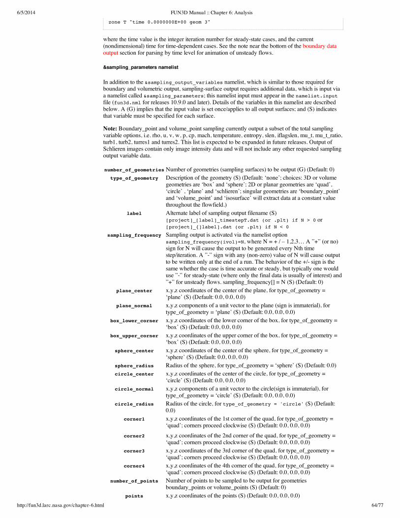
6/5/2014 FUN3D Manual :: Chapter 6: Analysis
http://fun3d.larc.nasa.gov/chapter-6.html 64/77
zone T "time 0.0000000E+00 geom 3"
where the time value is the integer iteration number for steady-state cases, and the current(nondimensional) time for time-dependent cases. See the note near the bottom of the boundary dataoutput section for parsing by time level for animation of unsteady flows.
&sampling_parameters namelist
In addition to the &sampling_output_variables namelist, which is similar to those required forboundary and volumetric output, sampling-surface output requires additional data, which is input viaa namelist called &sampling_parameters; this namelist input must appear in the namelist.inputfile (fun3d.nml for releases 10.9.0 and later). Details of the variables in this namelist are describedbelow. A (G) implies that the input value is set once/applies to all output surfaces; and (S) indicatesthat variable must be specified for each surface.
Note: Boundary_point and volume_point sampling currently output a subset of the total samplingvariable options, i.e. rho, u, v, w, p, cp, mach, temperature, entropy, slen, iflagslen, mu_t, mu_t_ratio,turb1, turb2, turres1 and turres2. This list is expected to be expanded in future releases. Output ofSchlieren images contain only image intensity data and will not include any other requested samplingoutput variable data.
number_of_geometriesNumber of geometries (sampling surfaces) to be output (G) (Default: 0)type_of_geometry Description of the geometry (S) (Default: ‘none’; choices: 3D or volume
geometries are ‘box’ and ‘sphere’; 2D or planar geometries are ‘quad’,‘circle’ , ‘plane’ and ‘schlieren’; singular geometries are ‘boundary_point’and ‘volume_point’ and ‘isosurface’ will extract data at a constant valuethroughout the flowfield.)
label Alternate label of sampling output filename (S)[project]_[label]_timestepT.dat (or .plt) if N > 0 or[project]_{]label].dat (or .plt) if N < 0
sampling_frequency Sampling output is activated via the namelist optionsampling_frequency(ivol)=N, where N = + / – 1,2,3… A ”+” (or no)sign for N will cause the output to be generated every Nth timestep/iteration. A ”-” sign with any (non-zero) value of N will cause outputto be written only at the end of a run. The behavior of the +/- sign is thesame whether the case is time accurate or steady, but typically one woulduse ”-” for steady-state (where only the final data is usually of interest) and”+” for unsteady flows. sampling_frequency[] = N (S) (Default: 0)
plane_center x,y,z coordinates of the center of the plane, for type_of_geometry =‘plane’ (S) (Default: 0.0, 0.0, 0.0)
plane_normal x,y,z components of a unit vector to the plane (sign is immaterial), fortype_of_geometry = ‘plane’ (S) (Default: 0.0, 0.0, 0.0)
box_lower_corner x,y,z coordinates of the lower corner of the box, for type_of_geometry =‘box’ (S) (Default: 0.0, 0.0, 0.0)
box_upper_corner x,y,z coordinates of the upper corner of the box, for type_of_geometry =‘box’ (S) (Default: 0.0, 0.0, 0.0)
sphere_center x,y,z coordinates of the center of the sphere, for type_of_geometry =‘sphere’ (S) (Default: 0.0, 0.0, 0.0)
sphere_radius Radius of the sphere, for type_of_geometry = ‘sphere’ (S) (Default: 0.0)circle_center x,y,z coordinates of the center of the circle, for type_of_geometry =
‘circle’ (S) (Default: 0.0, 0.0, 0.0)circle_normal x,y,z components of a unit vector to the circle(sign is immaterial), for
type_of_geometry = ‘circle’ (S) (Default: 0.0, 0.0, 0.0)circle_radius Radius of the circle, for type_of_geometry = 'circle' (S) (Default:
0.0)corner1 x,y,z coordinates of the 1st corner of the quad, for type_of_geometry =
‘quad’; corners proceed clockwise (S) (Default: 0.0, 0.0, 0.0)corner2 x,y,z coordinates of the 2nd corner of the quad, for type_of_geometry =
‘quad’; corners proceed clockwise (S) (Default: 0.0, 0.0, 0.0)corner3 x,y,z coordinates of the 3rd corner of the quad, for type_of_geometry =
‘quad’; corners proceed clockwise (S) (Default: 0.0, 0.0, 0.0)corner4 x,y,z coordinates of the 4th corner of the quad, for type_of_geometry =
‘quad’; corners proceed clockwise (S) (Default: 0.0, 0.0, 0.0)number_of_points Number of points to be sampled to be output for geometries
boundary_points or volume_points (S) (Default: 0)points x,y,z coordinates of the points (S) (Default: 0.0, 0.0, 0.0)

6/5/2014 FUN3D Manual :: Chapter 6: Analysis
http://fun3d.larc.nasa.gov/chapter-6.html 65/77
number_of_rows Number of pixels in window height (S) (Default: 0)number_of_columns Number of pixels in window width (S) (Default: 0)window_height Height of schlieren window (S) (Default: 0.0)window_width Width of schlieren window (S) (Default: 0.0)window_center x,y,z coordinates of the center of the schlieren window (S) (Default:
(0.,0.,0.)schlieren_aspect Window normal vector alignment, either y or z axes. (S) (Default: none
[blank])blanking_list_countNumber of boundaries to search to blank schlieren image (S) (Default: 0)blanking_list List of boundaries to search to blank schlieren image (S) (Default: none
[blank])isosurf_variable Flowfield variable used to visualize the iso-surface. (S) (Default: none
[blank])isosurf_value Value of the flowfield variable to be visualized. (S) (Default: 0)crinkle Plot output surface(s) as crinkle surface (G) (Default: .false. [smooth])
print_boundary_data Print data (for debugging?) (G) (Default: 0 [don’t print])snap_output_xyz When snap_output_xyz is true, the coordinates of the points output are
snapped to the boundary. When snap_output_xyz is false, the coordinatesof the points output come from the namelist input. (G) (Default: .true.)
dist_tolerance Distance, in mesh units, allowed to search for requested boundary pointdata. (G) (Default: 1.0e-3)
plot Choice of TECPLOT or Fieldview output (S) (Default: ‘tecplot’; alternate:‘fieldview’ or ‘serial_history’)
In the example below, two planes of data are output;
&sampling_parameters number_of_geometries = 2, type_of_geometry(1)='plane', ! start plane 1 data plane_center(1,1) = 3.5 ! x 2nd index is geom # plane_center(2,1) = 0.0 ! y plane_center(3,1) = 0.0 ! z plane_normal(1,1) = 1.0 ! xn plane_normal(2,1) = 0.0 ! yn plane_normal(3,1) = 0.0 ! zn type_of_geometry(2)='plane' plane_center(1,2) = 0.0 ! start plane 2 data plane_center(2,2) = 10.8333333333333 plane_center(3,2) = 0.0 plane_normal(1,2) = 0.0 plane_normal(2,2) = 1.0 plane_normal(3,2) = 0.0/
In the next example, a range of geometries are output; this example also depicts a slightly morecompact means of specifying the namelist data.
&sampling_parameters number_of_geometries = 10!-applies only to boundary_point sampling-- snap_output_xyz = .true. dist_tolerance = 0.1!------------------------------------------ type_of_geometry(1)='plane',sampling_frequency(1) = -1 plane_center(:,1)=4.0,0.0,0.0, plane_normal(:,1)=1.0,0.0,0.0,! type_of_geometry(2)='quad',sampling_frequency(2) = 1 corner1(:,2)=-2.0,-5.0, 6.0, corner2(:,2)=-2.0,-5.0,-6.0, corner3(:,2)=-2.0 ,5.0,-6.0, corner4(:,2)=-2.0, 5.0, 6.0,! type_of_geometry(3)='circle',sampling_frequency(3) = 5 circle_center(:,3) = 0.0, 0.0, 0.0, circle_normal(:,3) = 1.0, 0.0, 0.0, circle_radius(3) = 5.0,! type_of_geometry(4) ='box' sampling_frequency(4) = 0
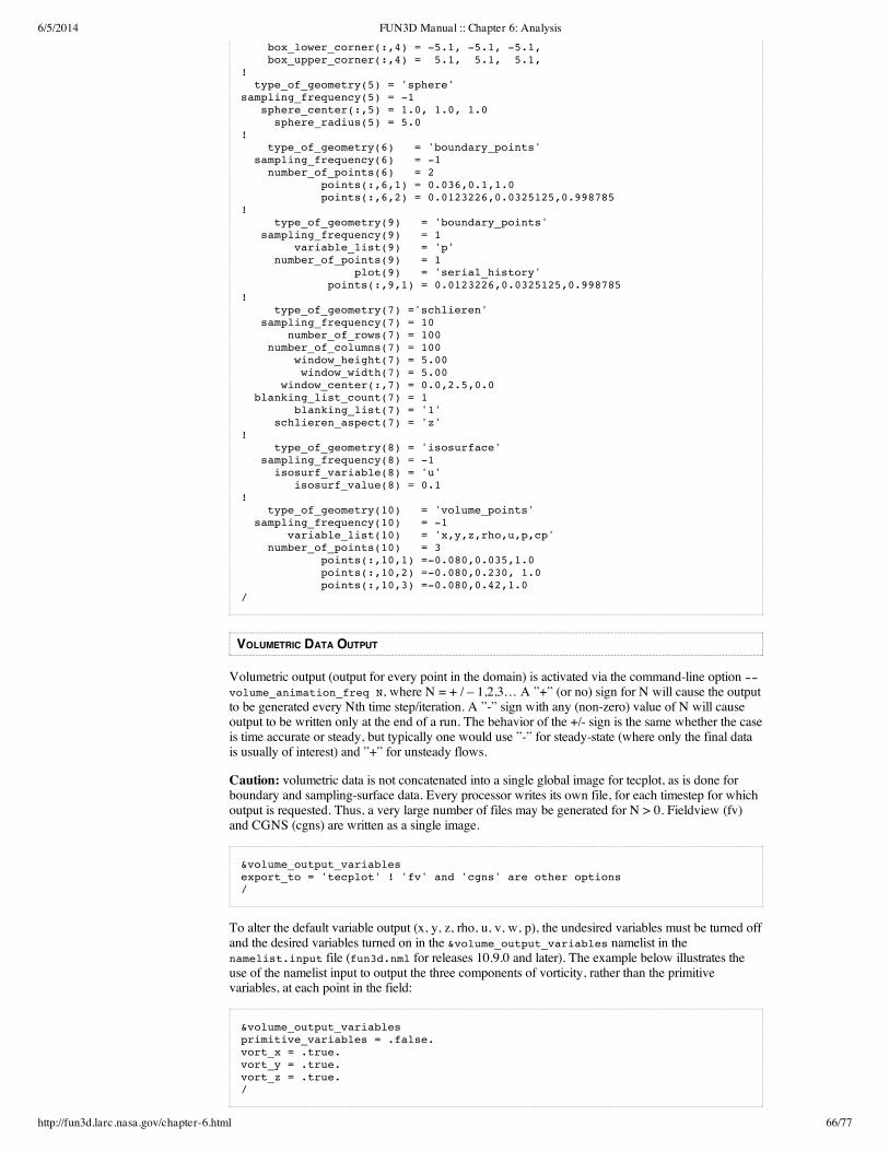
6/5/2014 FUN3D Manual :: Chapter 6: Analysis
http://fun3d.larc.nasa.gov/chapter-6.html 66/77
box_lower_corner(:,4) = -5.1, -5.1, -5.1, box_upper_corner(:,4) = 5.1, 5.1, 5.1,! type_of_geometry(5) = 'sphere' sampling_frequency(5) = -1 sphere_center(:,5) = 1.0, 1.0, 1.0 sphere_radius(5) = 5.0 ! type_of_geometry(6) = 'boundary_points' sampling_frequency(6) = -1 number_of_points(6) = 2 points(:,6,1) = 0.036,0.1,1.0 points(:,6,2) = 0.0123226,0.0325125,0.998785! type_of_geometry(9) = 'boundary_points' sampling_frequency(9) = 1 variable_list(9) = 'p' number_of_points(9) = 1 plot(9) = 'serial_history' points(:,9,1) = 0.0123226,0.0325125,0.998785! type_of_geometry(7) ='schlieren' sampling_frequency(7) = 10 number_of_rows(7) = 100 number_of_columns(7) = 100 window_height(7) = 5.00 window_width(7) = 5.00 window_center(:,7) = 0.0,2.5,0.0 blanking_list_count(7) = 1 blanking_list(7) = '1' schlieren_aspect(7) = 'z'! type_of_geometry(8) = 'isosurface' sampling_frequency(8) = -1 isosurf_variable(8) = 'u' isosurf_value(8) = 0.1! type_of_geometry(10) = 'volume_points' sampling_frequency(10) = -1 variable_list(10) = 'x,y,z,rho,u,p,cp' number_of_points(10) = 3 points(:,10,1) =-0.080,0.035,1.0 points(:,10,2) =-0.080,0.230, 1.0 points(:,10,3) =-0.080,0.42,1.0/
VOLUMETRIC DATA OUTPUT
Volumetric output (output for every point in the domain) is activated via the command-line option --volume_animation_freq N, where N = + / – 1,2,3… A ”+” (or no) sign for N will cause the outputto be generated every Nth time step/iteration. A ”-” sign with any (non-zero) value of N will causeoutput to be written only at the end of a run. The behavior of the +/- sign is the same whether the caseis time accurate or steady, but typically one would use ”-” for steady-state (where only the final datais usually of interest) and ”+” for unsteady flows.
Caution: volumetric data is not concatenated into a single global image for tecplot, as is done forboundary and sampling-surface data. Every processor writes its own file, for each timestep for whichoutput is requested. Thus, a very large number of files may be generated for N > 0. Fieldview (fv)and CGNS (cgns) are written as a single image.
&volume_output_variablesexport_to = 'tecplot' ! 'fv' and 'cgns' are other options/
To alter the default variable output (x, y, z, rho, u, v, w, p), the undesired variables must be turned offand the desired variables turned on in the &volume_output_variables namelist in thenamelist.input file (fun3d.nml for releases 10.9.0 and later). The example below illustrates theuse of the namelist input to output the three components of vorticity, rather than the primitivevariables, at each point in the field:
&volume_output_variablesprimitive_variables = .false.vort_x = .true.vort_y = .true.vort_z = .true./

6/5/2014 FUN3D Manual :: Chapter 6: Analysis
http://fun3d.larc.nasa.gov/chapter-6.html 67/77
Note that these variable selections in the &volume_output_variables namelist apply ONLY tovolumetric output. Other output (e.g. boundary data) will still contain default variables unless similarchoices are made in the appropriate namelist.
The resulting volume-data files will have the following naming convention:
[project]_partP_tec_volume_timestepT.dat (or .plt) if N > 0 [project]_PartP_tec_volume.dat (or .plt) if N < 0
where P = 1,2,...nproc (number of processors) and T is the time step or iteration number. Within thefiles, a single zone is written, with the zone identified as, for example:
zone T "time 0.0000000E+00 processor 32"
where the time value is the integer iteration number for steady-state cases, and the current(nondimensional) time for time-dependent cases. See the note near the bottom of the boundary dataoutput section for parsing by time level for animation of unsteady flows.
‘SLICED’ BOUNDARY DATA OUTPUT
A limited ability to take slices through boundary surfaces is available from within the flow solver.For example, spanwise cuts along a wing may be taken, and then the resulting pressure and skinfriction data may be plotted at each station. This capability largely parallels that of the box5/box6utility codes, with the added ability to handle unsteady flows in a simple fashion. This slicingcapability is also essential for (and in fact developed for) use in rotorcraft solutions where the flowsolver is coupled to an external Computational Structural Dynamics (CSD) code, such as CAMRAD.
Slices can only be taken at constant-coordinate positions (e.g. x=constant); for moving-body cases,the slices may be taken at constant-coordinate positions in a body-fixed coordinate system, in whichcase the slices will not generally be in constant coordinate planes in inertial space.
The sliced data is written to an ASCII formatted TECPLOT file with the naming convention:
{project}_slice.tec
The variables output to this file are: x, y, z, cp, cfx, cfy, cfz at each output time step. Note that unlikethe solver-output options described in the previous sections, the output variables from boundary-surface slicing are not customizable by the user.
Slicing occurs in the inertial frame unless an alternate reference frame is specified. For stationarygeometries, the inertial frame is the only option. For moving body cases, either the frame of one of themoving bodies (see Defining Moving Bodies) or an observer frame (see Specifying ObserverMotion) may be more appropriate.
Surface data slicing is enabled within the flow solver with the command line option: --slice_freqINT where INT is the (integer) frequency at which the boundary data is sliced. The --slice_freqoption operates exactly as --animation_freq
In addition to this command line option, specific instructions on where to take the slices must beprovided through the namelist &slice_data, which in Version 11.1 and higher is input viafun3d.nml (in earlier versions of the code, this namelist was set via a file calledslice_global_bndry.input)
An (S) following a variable description implies that the data may be specified for each slice; a (G)implies the data applies to all slices
&slice_data namelist
nslices Number of slices to create (G) (Default: 0); if negative, then data foronly one slice station need be input, along with a spacing increment,and all the data specified for the first station will be applied tosubsequent stations, with the exception of the slice location, which willbe set using the spacing increment
slice_increment Increment in slice location between consecutive slice stations (G)(Default: 0.0); to be utilized with nslices < 0, in which case the valueshould be explicitly set, as the default increment will place all slices atthe same location as the first slice; if nslices > 0, the value ofslice_increment is unused
tecplot_slice_output Output the sliced data (coordinates, Cp, Cf, etc) to a (formatted)

6/5/2014 FUN3D Manual :: Chapter 6: Analysis
http://fun3d.larc.nasa.gov/chapter-6.html 68/77
Tecplot file, [project]_slice.dat, for animation. Caution: for unsteadyflows with frequently written data at many slice locations, this file canbecome very large. (G) (Default: .true.)
output_sectional_forcesOutput detailed force and moment data for each slice to a (formatted)file, [project].sectional_forces; this file contains F/M data like that inthe [project].forces file, only for each and every slice. In addition, itcontains geometrical data for each slice (le/te coordinates, momentcenter, etc.) Caution: for unsteady flows with frequently written dataat many slice locations, this file can become very large. On the otherhand, the data in the file, especially the geometry data, can be useful toassess whether the slicing is working as expected (G) (Default: .true.)
slice_frame Name of the reference frame in which slice is to be taken (S) (Default:’’ [indicates inertial frame] ); for moving geometries, to specify theobserver frame, use ‘observer’; to specify the frame of a particularbody, use ‘body_name’, where body_name is that specified in the&body_definitions namelist
replicate_all_bodies An “easy button” to set similar slice stations on multiple bodies withminimal input beyond that required for slicing the first body.Particularly useful for rotorcraft applications where multiple blades areto be sliced. This variable duplicates the input slice info for all movingbodies, with the exception of slice_frame and thebndrys_to_slice data (G) (Default: .false.)
slice_x Slice to be taken normal to x-direction (i.e. at x=constant) in thespecified reference frame (S) (Default: .false.)
slice_y Slice to be taken normal to y-direction (i.e. at y=constant) in thespecified reference frame (S) (Default: .true.)
slice_z Slice to be taken normal to z-direction (i.e. at z=constant) in thespecified reference frame (S) (Default: .false.)
slice_location Coordinate value at which slice is taken (S) (Default: 0.0)n_bndrys_to_slice Number of candidate boundaries to search while computing slice-
plane intersections (S) (Default: all solid boundaries). Specifyingwhich boundaries are candidates for slicing may speed up the slicingprocess; may also be used to filter out unwanted intersections or toslice non-solid boundaries
bndrys_to_slice List of n_bndrys_to_slice boundaries that will be searched to computethe slice-plane intersection (S) (Default: all solid boundaries)
slice_group Assign this slice to a particular group number; within a group, slicelocations are expected to be given in ascending order; multiple slicegroups can be used to circumvent this (S) (Default: 1)
te_def number of points or line segments to consider when defining the“trailing edge” of the slice; a) a value of +1 defines the TE as the aft-most point – best for sharp trailing edges; b) a positive number > 1initiates a search, over the aft-most te_def segments for “corners”, afterwhich the TE is taken as the average coordinate over all the detectedcorners – 2 corners are assumed to be the desired number andwarnings are output if only 1 or more than 2 are found. Note that thevalue of te_def must be chosen judiciously – large enough to allowboth corners to be found, but not so large as to cause excessivesearching or for any non-trailing edge corners to be found - this optionis best for and recommended only for squared-off trailing edges; c) anegative number indicates a parabolic fit of the aft-most abs(te_def)points – best for rounded/blunted trailing edges (S) (Default: +1 –declare the aft-most point as the trailing edge)
le_def number of points to consider when defining the “leading edge” of theslice; a) a value of +1 defines the TE as the forward-most point – use ifnothing else works or for special cases; b) a positive number indicatesa search over the forward-most le_def points for the one that has themaximum distance from the previously-determined trailing edge –generally the best choice provided the trailing edge can be accuratelylocated; c) a negative number indicates a parabolic fit over theforward-most abs(le_def) points (S) (Default: +30 – search the 30forward-most points to find the one that has the maximum distancefrom the previously-determined trailing edge)
corner_angle used in conjunction with te_def > 1; angles between adjacent slicedsegments that are less than the corner_angle value will be consideredas indicative of a corner between the two segments. For squared-offtrailing edges, two and only two corners should be detected. (Default:

6/5/2014 FUN3D Manual :: Chapter 6: Analysis
http://fun3d.larc.nasa.gov/chapter-6.html 69/77
120 – angles less than 120 degrees are considered corners)chord_dir Direction of local chord relative to the direction from leading edge to
trailing edge; +1 indicates local chord in direction le -> te; -1 indicateslocal chord in direction te -> le (S) (Default: +1)
use_local_chord Use the computed local (sectional) chord, based on the computed LEand TE locations, to normalize the sectional force and moment data;otherwise the input value of Cref will be used. (G) (Default: .true.)
slice_xmc x-coordinate of the moment center in the specified reference frame (S)(Default: computed “quarter chord” of the slice)
slice_ymc y-coordinate of the moment center in the specified reference frame (S)(Default: computed “quarter chord” of the slice)
slice_zmc z-coordinate of the moment center in the specified reference frame (S)(Default: computed “quarter chord” of the slice)
xx_box_min Minimum x-coordinate used to define a bounding box to constrain theslicing. (S) (Default: negative huge number – i.e. no bounding)Specifying bounding box surfaces can aid in filtering out unwantedintersections
xx_box_max Maximum x-coordinate used to define a bounding box to constrain theslicing. (S) (Default: positive huge number – i.e. no bounding)
yy_box_min Minimum y-coordinate used to define a bounding box to constrain theslicing. (S) (Default: negative huge number – i.e. no bounding)
yy_box_max Maximum y-coordinate used to define a bounding box to constrain theslicing. (S) (Default: positive huge number – i.e. no bounding)
zz_box_min Minimum z-coordinate used to define a bounding box to constrain theslicing. (S) (Default: negative huge number – i.e. no bounding)
zz_box_max Maximum z-coordinate used to define a bounding box to constrain theslicing. (S) (Default: positive huge number – i.e. no bounding)
When slicing boundary surfaces, a file called slice.info is output that echos much of the aboveinput data in more-or-less plain English; assuming the first pass through the slicing routines issuccessful, the file will also contain information about the number of points in the slice, etc.
Important Considerations for Determination of Leading And Trailing Edges
This is especially important for rotorcraft applications where airloads are usually examined (andprovided to a CSD code, if applicable), in a section-aligned coordinate system.
The leading and trailing edge points determine the orientation of a section-aligned coordinate system;when slicing boundary data, the computed forces are computed in both the selected frame ofreference, and in a section-aligned system. If the data in the section-aligned system is irrelevant toyou, then you do not need to worry about choosing the detection parameters carefully – the defaultvalues should do something semi-reasonable, without complaint, in most situations.
However, if resolution of forces and moments into a section-aligned system is important to you thenthere are a number of things to consider:
1) Make sure the chord direction (chord_dir) is correct; the default is that going from the LE to the TEis the same as traveling in the positive “chordwise” coordinate direction. For most applications this usthe usual situation, however for rotorcraft applications this will generally not be the case (seecomponent_blade_orientation) and you will want to set chord_dir = -1
2) Since the best option for determining the LE uses the TE location (le_def > +1), then care shouldbe taken to get the TE correct. For sharp trailing edges, this is very simple since the default of te_def= +1 (i.e. use the aft-most point) is the best option. However, smoothly blunted or squared-off trailingedges are more finicky. Note that when the boundary surface of an unstructured mesh is sliced, theresulting section will be comprised of line segments determined by the intersection of the specifiedplane and the edges of the surface triangles. These segments and the points that make up the segmentswill not usually be the same as the surface points - typically there are more, as illustrated in thefollowing two figures. Bear this in mind when setting te_def and le_def values. You will needenough segments to ensure that both corners are detected, bit not so many that other, non trailing-edge corners (if present) are detected. Another parameter that may be of use to aid in the detection ofcorners is the corner_angle; the default is 120 degrees (so an angle between segments < 120 degreesindicates a corner), and this seems quite reasonable for all cases considered so far, but unusualsituations may require a different value.

6/5/2014 FUN3D Manual :: Chapter 6: Analysis
http://fun3d.larc.nasa.gov/chapter-6.html 70/77
Above: View looking upstream from the trailing edge of a rotor blade mesh; the light-colored regionis the squared-off trailing edge; the red line shows the location where an x=const slice will be taken;black circles indicate surface grid points that sit on the trailing edge.
Above: The resulting sliced section, zoomed in to the trailing edge region; the aft-most 8 segments (ofthe approx. 30 segments in this view) are shown in red. The computed trailing edge locations usingtwo different te_def values are shown. The minimum te_def value at this particular station to pick upboth corners would be 8, but a value of 20 was used to be safe and to allow for any station-to-stationvariations. Note that if the blade was pitched downward rather than upward, then the point chosen byte_def = 1 would be the lower corner, rather than the upper. Thus, when pitching up and down,te_def = 1 with squared-off trailing edges can lead to jumps in the trailing edge position as the sectiontransitions from pitch up to pitch down. Depending on the thickness of the trailing edge, this can leadto jumps in the geometric pitch angle of a few tenths of a degree.
3) Smoothly-blunted (rounded) trailing edges should be done with either te_def = 1 (aft-most point)or via a parabolic fit of the aft-most abs(te_def) points; the latter option is probably better in generalbut will require some experimentation for the particular case at hand to choose the optimal number ofpoints over which to fit the parabola.
4) The leading edge is typically easier to determine, again assuming a good trailing edge position hasalready been found. The default value of le_def = +30 (search the 30 forward-most points for the onefurthest from the trailing edge) should do a decent job for most cases.

6/5/2014 FUN3D Manual :: Chapter 6: Analysis
http://fun3d.larc.nasa.gov/chapter-6.html 71/77
Above: A sliced section, zoomed in to the leading edge region; the forward-most 20 segments (of theapprox. 30 segments in this view) are shown in red. The computed leading edge locations using twodifferent le_def values are shown. In this case, both results are fairly close but le_def = 30 has pickedout the true leading edge (as judged from the LE geometry at zero pitch angle).
5) Given that the leading edge and trailing edge detection schemes can be somewhat finicky, forcases that rely on accurate resolution of forces and moments into section-aligned coordinates (e.g.rotorcraft), then it is wise to spend some time up front to make sure that things are coming out asexpected. To do this, inspect the [project].sectional_forces file for a particular slice station; at eachstation the computed leading and trailing edge coordinates will be output. Plot the correspondingstation from the [project]_slice.dat, as done above, and make sure the computed coordinates are thecorrect ones. If many stations are sliced, it is impractical to inspect all of them in this manner, but it isgood practice to spot check at least a few stations. For moving-geometry cases, try first running thecase with—body_motion_only. That will allow output of the [project].sectional_forces and[project]_slice.dat files without the expense of a flow solve or mesh deformation; for spot checkingyou may want to have the slicing done infrequently, and perhaps with fewer stations than ultimatelydesired, as these output files can be huge.
6) While the [project].sectional_forces can be useful for spot checking, the data in the file is not in aformat that is amenable to plotting. The FUN3D/utils/Rotorcraft directory contains a utility code thatwill read in the [project].sectional_forces and slice.info files and output TECPLOT files, for eachslice group, containing force/moment data in the section-aligned coordinate system, as well asgeometry data (LE, TE, and quarter-chord coordinates, and pitch angle).
7) After making sure that the LE and TE positions are being computed correctly, you may want toturn off one or both of the [project].sectional_forces and [project]_slice.dat files unless needed. Forinstance, in rotorcraft applications with coupling to external CSD codes, although the blade boundarysurfaces must be sliced to generate the aerodynamic loads data for the CSD code, this information isactually passed to the CSD code by another file; the [project].sectional_forces and [project]_slice.datfiles are not used.
8) Although the slicing process will work for multi-element airfoils, at this time the computation ofthe LE and TE is only done for the entire section, not each element individually.
6.11. INDIVIDUAL COMPONENT FORCE TRACKING
This section describes how to obtain force and moment history files of groups of boundaries.
This capability is available in Version 11.4 and higher.
This capability is not currently available for the Generic Gas Option.
Beginning with Version 11.4, all of the options below may be used with the&component_parameters namelist within the fun3d.nml file. This will allow generation ofindividual tracking of groups of boundaries and is activated with the command line option of --track_group_forces..
General InformationNamelist Format

6/5/2014 FUN3D Manual :: Chapter 6: Analysis
http://fun3d.larc.nasa.gov/chapter-6.html 72/77
GENERAL INFORMATION
The individual component forces contain the three forces and moments and forces for each groupingof boundaries in addition to massflow, average velocity and pressure when requested.
The resulting component history files will have the following naming convention:
[project]_[component_name]_component.dat
and are written to every iteration the same as the [project]_hist.dat file. The files are in TECPLOTformat.
By default, the variables that are output are
Iteration [iteration number]C<sub>x</sub> [axial force]C<sub>y</sub> [lateral force]C<sub>z</sub> [normal force]C<sub>M,x</sub> [moment around x-axis]C<sub>M,y</sub> [moment around y-axis]C<sub>M,z</sub> [moment around z-axis]
For flow-through boundaries,
Mass flow [mass flow through the boundary]<greek>r</greek> [average density]u [average velocity]p/p<sub>0</sub> [average normalized pressure] T [average temperature] p<sub>t</sub>/p<sub>0</sub> [average normalized total pressure] T<sub>t</sub> [average total temperature] Mach [average Mach number]
are also calculated and written to the component history file. All flow-through quantities are area-weighted averages.
NAMELIST FORMAT
number_of_component Number of groupings of boundaries to be output (G) (Default: 0)component_count Number of boundaries to be grouped.(S) (Default: 0)component_input String containing the boundary numbers for the group (S) (Default:
none [blank string])component_name Name of component grouping (S) (Default: none [blank string])
allow_flow_through_facesAllows calculation of flow-through quantities. (G) (Default: .false.)
NOTE: Flow through boundaries, including but not limited to 7011 (subsonic_inflow_pt), 5051(back_pressure), 5052 (subsonic_outflow_mach), 7031 (massflow_out), 7036 (massflow_in) requireallow_flow_through_forces to be set to .true. if mass flow and other average flow quantities areto be calculated..
In the example below, data are gathered for four groupings of boundaries;
&component_parameters number_of_components=4 component_count(1)=9 component_input(1)='1,2,3,4,5,6,7,8,9' component_name(1)='airplane'! component_count(2)=2 component_input(2)='2,3' component_name(2)='wing'! component_count(3)=3 component_input(3)='4,5,6' component_name(3)='engine1'! component_count(4)=3 component_input(4)='7,8,9' component_name(4)='engine2' allow_flow_through_forces = .true.

6/5/2014 FUN3D Manual :: Chapter 6: Analysis
http://fun3d.larc.nasa.gov/chapter-6.html 73/77
/
6.12. STATIC GRID TRANSFORMS
Occasionally the situation arises in which a grid is in hand, but the orientation of the grid isinappropriate for the desired simulation. In such a situation, a static-grid transform may be applied tothe grid before the flow solution is started. The original grid file is not changed by this transform – thesame input/command line options for transformation must be applied for any subsequent restarts.
To invoke a static transform, the command line option --grid_transform must be specified. Inaddition, details of the transform must be prescribed in the fun3d.nml file via the grid_transformnamelist.
&grid_transform namelist
ds Displacement magnitude for translation (Default: 0.0)sx X-component of unit vector along translation axis (Default: 1.0)sy Y-component of unit vector along translation axis (Default: 0.0)sz Z-component of unit vector along translation axis (Default: 0.0)theta Rotation angle (degrees) (Default: 0.0)tx X-component of unit vector along rotation axis (Default: 1.0)ty Y-component of unit vector along rotation axis (Default: 0.0)tz Z-component of unit vector along rotation axis (Default: 0.0)scale Scale factor applied to grid (Default: 1.0)
transform4×4 transform matrix as a means to specify more general transforms than can beaccommodated by the parameters listed above; specification of a transform matrix(except for an identity matrix) supersedes all other variables in the namelist (Default:identity matrix)
The transform matrix is described on pp 6-7 in the paper Recent Enhancements To The FUN3DFlow Solver For Moving-Mesh Applications The 4th row of the matrix should always be (0,0,0,1).
Rotations direction follows the right-hand rule along the rotation axis.
When specifying a static grid transform, the user should be cognizant of potential boundary conditionissues, particularly with regard to symmetry conditions. If symmetry conditions are used, possiblerotations are limited. For example, if a standard wing grid with a y=constant symmetry plane at thewing root (with BC 6662) is pitched about the y-axis, the symmetry condition is unchanged.However, if that same grid is rotated about the x-axis, by say, 30 degrees, then what was a y-constantplane is no longer on a constant-coordinate plane, and the code will fail. However, if the rotation wasinstead 90 degrees, then the y=constant plane would become a z=constant plane, for which theappropriate BC is 6663. In such a situation, where one type of constant-coordinate symmetry planebecomes another constant-coordinate symmetry plane, the flow solver will automatically swap theBCs. These situations require that precise +/- 90 degree rotations be specified.
A static transform may also be combined with the mirroring options to obviate some types ofsymmetry-plane issues. Mirroring is applied first (removing the symmetry plane), after which themirrored grid is transformed.
For example, the 30 degree roll case described above could be accommodated with --grid_transform --mirror_y and the appropriate namelist data.
Original grid

6/5/2014 FUN3D Manual :: Chapter 6: Analysis
http://fun3d.larc.nasa.gov/chapter-6.html 74/77
After mirroring and rotation using either
&grid_transform theta = 30.0 tx = 1.0 ty = 0.0 tz = 0.0 /
or, directly specifying the transform matrix
&grid_transform transform(1,1) = 1.0 transform(1,2) = 0.0 transform(1,3) = 0.0 transform(1,4) = 0.0 transform(2,1) = 0.0 transform(2,2) = 0.86602540E+00 transform(2,3) = -0.5 transform(2,4) = 0.0 transform(3,1) = 0.0 transform(3,2) = 0.5 transform(3,3) = 0.86602540E+00 transform(3,4) = 0.0 transform(4,1) = 0.0 transform(4,2) = 0.0 transform(4,3) = 0.0 transform(4,4) = 1.0 /
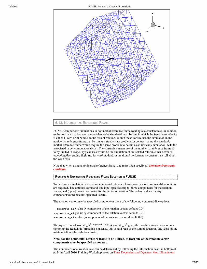
6/5/2014 FUN3D Manual :: Chapter 6: Analysis
http://fun3d.larc.nasa.gov/chapter-6.html 75/77
6.13. NONINERTIAL REFERENCE FRAME
FUN3D can perform simulations in noninertial reference frame rotating at a constant rate. In additionto the constant rotation rate, the problem to be simulated must be one in which the freestream velocityis either 1) zero or 2) parallel to the axis of rotation. Within these constraints, the simulation in thenoninertial reference frame can be run as a steady state problem. In contrast, using the standard,inertial reference frame would require the same problem to be run as an unsteady simulation, with theassociated larger computational cost. The constraints mean use of the noninertial reference frame isfairly limited in scope. Typical uses would be the simulation of an isolated rotor in either hover orascending/descending flight (no forward motion), or an aircraft performing a constant-rate roll aboutthe wind axis.
Note that when using a noninertial reference frame, one must often specify an alternate freestreamcondition
RUNNING A NONINERTIAL REFERENCE FRAME SOLUTION IN FUN3D
To perform a simulation in a rotating noninertial reference frame, one or more command-line optionsare required. The optional command-line input specifies (up to) three components for the rotationvector, and (up to) three coordinates for the center of rotation. The default values for anycomponent/coordinate not specified is zero.
The rotation vector may be specified using one or more of the following command-line options:
--xrotrate_nixvalue (x-component of the rotation vector; default: 0.0)--yrotrate_niyvalue (y-component of the rotation vector; default: 0.0)--zrotrate_nizvalue (z-component of the rotation vector; default: 0.0)
The square root of xrotrate_ni2^ + yrotrate_ni2^ + zrotrate_ni2 gives the nondimensional rotation rate(ignoring the RedCloth formatting nonsense, this should read as the sum of squares). The sense of therotation follows the right-hand rule.
Note: for the noninertial reference frame to be utilized, at least one of the rotation vectorcomponents must be specified as nonzero.
The nondimensional rotation rate can be determined by following the information near the bottom ofp. 24 in April 2010 Training Workshop notes on Time-Dependent and Dynamic-Mesh Simulations

6/5/2014 FUN3D Manual :: Chapter 6: Analysis
http://fun3d.larc.nasa.gov/chapter-6.html 76/77
The rotation vector passes through an origin whose coordinates are specified using one of more of thefollowing command-line options:
--xrotcen_nixvalue (x-coordinate of the rotation vector; default: 0.0)--yrotcen_niyvalue (y-coordinate of the rotation vector; default: 0.0)--zrotcen_nizvalue (z-coordinate of the rotation vector; default: 0.0)
These values are specified in terms of grid coordinates.
As an example, suppose you have a rotor in hover, rotating about the z-axis, with a nondimensionalrotation rate of 0.00272. Then all that is required to specify the noninertial rotation is the command-line:
--zrotrate_ni 0.00272
This minimal input takes advantage of the zero defaults for all noninertial data that is not explicitlyspecified.
If the same rotation vector was desired, but with the rotation centered about a point x=0.25 y=0.75 inthe x-y plane, use the command line:
--zrotrate_ni 0.00272 --xrotcen_ni 0.25 --yrotcen_ni 0.75
(the center of rotation in the z direction is immaterial for rotations about an axis parallel to the z-axis,so the implied default 0 is used)
If the solution from a noninertial case is output for viewing, the relative velocities in the noninertialframe are output to the file (assuming you choose to output the velocity components). Thus, theoutput velocity will be zero on solid surfaces, and on farfield boundary surfaces will have an oppositesense to the direction of rotation in inertial space, as illustrated below on an outflow plane for a rotorwith a counterclockwise rotation about the z-axis when viewed from above.
SPECIFYING AN ALTERNATE FREESTREAM CONDITION
In FUN3D, by default the freestream conditions (velocity components) for compressible flow are setby the Mach number, angle of attack, and yaw angles specified in the fun3d.nml file. Forcompressible flows, an input Mach number of 0 will quickly lead to numerical disaster, since theviscous terms scale inversely with Mach number (for incompressible flow, scaling does not dependon the Mach number). Likewise, the unit Reynolds number should correspond to the velocityassociated with the input Mach number.
Consider a rotor in hover. In this case the freestream velocity is zero, but if we are running acompressible simulation, we cannot have an input Mach number of zero. In addition, thecorresponding unit Reynolds number should not be based on zero velocity.
The solution is to base the input Mach number on a more sensible velocity, say the rotor tip speed(and base the unit Reynolds number on this same reference speed). Since we still need zero velocityin the freestream, the --alternate_freestream command line option is used to override thefreestream velocity corresponding to the input Mach number:
--alternate_freestream 0.0
Previous (C5: Pre/Post Processing) | Up | Next (C7: Adaptation and Error Estimation)

6/5/2014 FUN3D Manual :: Chapter 6: Analysis
http://fun3d.larc.nasa.gov/chapter-6.html 77/77
Today's NASA Official: Mike Park, a member of The FUN3D Development TeamContact: [email protected] Privacy Statement
This material is declared a work of the U.S. Government and is not subject to copyright protection in theUnited States.