6 final technical report - department of computer sciencemisha/fall05/papers/chen95.pdf · 6 final...

Final Technical Report 5

2 Description of Complex Objectsfrom Multiple Range Images Using

an Inflating Balloon ModelYang Chen and Gérard Medioni

We address the problem of constructing a complete surface model of an object us-ing a set of registered range images. The construction of the surface description is car-ried out on the set of registered range images. Our approach is based on a dynamicballoon model represented by a triangulated mesh. The vertices in the mesh arelinked to their neighboring vertices through springs to simulate the surface tension,and to keep the shell smooth. Unlike other dynamic models proposed by previous re-searchers, our balloon model is driven only by an applied inflation force towards theobject surface from inside of the object, until the mesh elements reach the object sur-face. The system includes an adaptive local triangle mesh subdivision scheme that re-sults in an evenly distributed mesh. Since our approach is not based on globalminimization, it can handle complex, non-star-shaped objects without relying on acarefully selected initial state or encountering local minimum problem. It also allowsus to adapt the mesh surface to changes in local surface shapes and to handle holespresent in the input data through adjusting certain system parameters adaptively.We present results on simple as well as complex, non-star-shaped objects from realrange images.

2.1 IntroductionThe task of surface description using 3-D input can be described as finding a fit

of a chosen representation (model surface) to the input data. This process can be for-malized in a number of ways involving the minimization of a system functional thatexplicitly or implicitly represents the fit of the model to the input data. Another veryimportant aspect of such a system is to construct a mapping or correspondence be-tween the surface of an object and the structure of the model. This mapping exists be-cause the surface of the model and the surface of the object are topologicallyequivalent, considering genus zero type of objects. Therefore there exists a one-to-onemapping between the model structures and the object surface elements. Previous re-searchers have studied such mappings in a variety of ways using different represen-tation schemes and model fitting methods. Examples of these approaches include thedynamic system using energy minimization in [4] and the dynamic mesh in [12] and[13]. The drawbacks of these approaches is that they must rely on an initial guess ofthe model structure which is relatively close to the shape of the object. The reason isthat, in the absence of mapping or correspondence information, some other approxi-

6 Final Technical Report

mations have to be used, such as the nearest data point to the model [13] in order forthe system to converge to the desired results under the attraction force between thecorrespondence points in the model and the data. Such an approximation would haveproblems in cases where there are data points that are not the closest to their truecorresponding points of the model, and thus inevitably lead the system towards a sub-optimal situation (local minimum). This is why those approaches can only deal withstar-shaped objects.

In this paper we present a new approach for surface description using a dynamicballoon model represented by a triangular mesh. We start with a small triangulatedshell placed inside the object and apply a uniform inflation force on all vertices in thedirection normal to the shell’s surface. The vertices are also linked to their neighbor-ing vertices through springs to simulate the surface tension and to keep the shellsmooth. The applied inflation force moves the vertices towards the object surface untilthey “land” on it. This process is similar to that of blowing up a balloon placed insidethe hollow object until it fits the shell of the object. Thus the goal of mapping the mod-el to the object surface is achieved through the physics of a growing balloon in a verynatural way (see Figure 2.1 ). Of course, we also need to handle noisy data, and holes(lack of data), as described later.

Our system is not based on global minimization methods, and it can make deci-sions based on local information about the shape of the object surface. During the pro-cess of the growth of the triangular mesh, the triangles will be subdivideddynamically to reduce spring tension and to allow the mesh surface area to increasein order to cover the larger object surface. As the mesh expands and the vertices startto reach the object surface, the entire mesh surface is gradually subdivided into pieces

Figure 2.1 The inflating balloon model as illustrated in a 2-D case: (a)the initial state, (b) and (c) intermediate states, (d) the final state.

(a) (b)

(c) (d)


of connected triangular regions, which allows us to treat the surfaces in a local contextby tailoring the parameters, and possibly strategy, of the system in dealing with eachregion separately based on local information.

Another aspect of our approach is its role in data integration. Most of the previ-ous research make use of scattered 3-D points or a single range image as input. Veryfew researchers (e.g. [10]) try to use multiple densely sampled range images. Thereare two difficulties in using these range images. First the images must be preciselyregistered. We have previously presented a method [1] to register multiple range im-ages, which is used to register the range images used in this paper. The second is theissue of integration. Integration can not be performed without an appropriate repre-sentation for the integrated data. While star-shaped objects can be simply mappedonto a unit sphere, and the integration can then be performed easily [1]. This is nottrue for complex objects, since it is difficult to find an integrated representation. Thusfinding a suitable representation is very important. While it is not the main theme ofthis paper, we believe that our approach leads to a good solution to combine and takeadvantage of multiple range images in surface description for complex objects interms of integration.

In the following sections, we first review some of the related previous work andthen present our balloon model in detail. Section [2.3] describes our surface model andhow it works, Sections [2.4] and [2.5] define the dynamics of the system. Section [2.6]explains the adaptive mesh subdivision scheme. In Sections [2.7] and 8, we give analgorithmic description of our system and describe how to set system parameters. Sec-tion Chapter 2 discusses issues on how to adapt the parameters locally and dealingwith noise. Several test results from real range images, from both simple and complexobjects, are presented in Section [2.10]. The conclusion follows in Section [2.11].

2.2 Related WorkDynamic mesh models have been proposed by previous researchers for shape de-

scription. [12] introduced a shape reconstruction algorithm using a dynamic meshthat can dynamically adjust its parameters to adapt to the input data. [13] then ex-tended this approach by introducing an attraction force from the 3-D input for shapedescription. [6] also proposed a similar system with dynamic nodal addition/deletionfor shape description and nonrigid object tracking. [4] proposed a deformable modelwith both internal smoothness energy and external forces from both the input dataand features. There exist other deformable model approaches that differ in the repre-sentation schemes of the model and in the approaches to solving the system [5][11].

The main difference between our method and those used by previous research-ers is that we do not explicitly introduce a data force into our model, as discussed indetails in the following sections. Our model is driven by an inflation force introducedinside the balloon. Balloon models have been used by [3] and [7], but in these ap-


proaches, the introduced balloon force is used mostly to overcome noise in the data sothat the system can converge to the desired results more easily.

2.3 The Inflating Balloon ModelOur balloon model is represented by a shell of triangulated patches. The initial

triangulated shell is an icosahedron. A triangulated shell can be either considered asa mesh consisting of triangular patches or a mesh consisting of vertices (or nodes) con-nected to their neighbors. In the following discussion, a mesh element may refer toeither a vertex or a triangle patch. But in this paper, we mainly explore the propertiesof the vertices.

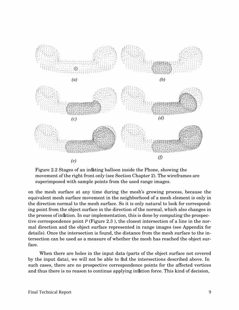
When placed inside the object, and under the influence of the inflation force, theshell grows in size as the vertices move along the mesh surface normal in the radialdirection, maintaining an isotropic shape, until one or more vertices reaches the ob-ject surface. During the process of inflation, the triangles may be subdivided adaptive-ly, which also creates new vertices. Once it reaches the surface, a vertex is consideredanchored to the surface and thus can no longer move freely. The remaining vertices,under the influence of the anchored vertices, will gradually change their course ofmovement, until finally reaching their corresponding surface point. As can be seenfrom this process, the movement of the vertices is not influenced directly by any forcefrom the surface of the object. This seems to be bad from the viewpoint of a fitting pro-cess, which tries to minimize some distance measure between the object surface andthe model. But this is important to us because our main concern is to find the mappingbetween the mesh elements and the object surface. Not using any attraction forcefrom the surface data allows us to avoid incorrect mappings, which is a similar situ-ation to the local minimum problem in energy minimization approaches. An exampleof the growing balloon is shown in Figure 2.2 .

2.3.1 The Correspondence Problem

So far, we have not discussed how to test whether the mesh has reached the sur-face of the object. This is the key difference between our approach and other dynamicmodel systems or energy minimization systems. In order to test whether a vertex hasreached the object surface, one must measure the distance between the mesh surfaceand some point on the object surface. Ideally this point on the object surface shouldbe the corresponding point of the vertex, which is not possible before the vertex reach-es the surface. Previous researchers have used the closest point on the object surfaceto an mesh element as an alternative, but it may provide incorrect information. In [7]the distance from the data points on the surface to the nearest model point is usedinstead, which is an improvement over the above approach. This approach, however,is not practical when there is a large number of surface sample points from the object,as in our case.

In our approach, we look for potential corresponding points only in the directionnormal to the mesh surface. This is the best knowledge locally available to the points


on the mesh surface at any time during the mesh’s growing process, because theequivalent mesh surface movement in the neighborhood of a mesh element is only inthe direction normal to the mesh surface. So it is only natural to look for correspond-ing point from the object surface in the direction of the normal, which also changes inthe process of inflation. In our implementation, this is done by computing the prospec-tive correspondence point P (Figure 2.3 ), the closest intersection of a line in the nor-mal direction and the object surface represented in range images (see Appendix fordetails). Once the intersection is found, the distance from the mesh surface to the in-tersection can be used as a measure of whether the mesh has reached the object sur-face.

When there are holes in the input data (parts of the object surface not coveredby the input data), we will not be able to find the intersections described above. Insuch cases, there are no prospective correspondence points for the affected verticesand thus there is no reason to continue applying inflation force. This kind of decision,

Figure 2.2 Stages of an inflating balloon inside the Phone, showing themovement of the right front only (see Section Chapter 2). The wireframes aresuperimposed with sample points from the used range images.

(a) (b)

(c) (d)

(e)(f)


however, should not be made locally for each vertex point. We will discuss the han-dling of holes when we discuss our algorithm in details later, in Section [2.8].

2.4 A Simplified Dynamic ModelThe motion of any element i on the model surface can be described by the follow-

ing motion equation [12]:

(2.1)

where xi is the location of the element, and are the first and second deriva-tives with respect to time, mi represents the mass, ri is the damping coefficient, gi isthe sum of internal forces from neighboring elements due to, e.g., spring attachmentsand fi is the external force exerted on the element. Because of the nonlinear nature ofthe forces gi and fi involved, the systems of ordinary differential equations in Equa-tion (2.1) can be solved using explicit numerical integration [12].

The dynamic system will reach the equilibrium state when both and be-come 0, which can take a very long time since it is usually an exponential process. Asimplified system can be obtained if we make mi = 0, and ri = 1 for all i, in which caseEquation (2.1) reduces to

(2.2)

There are several reasons for this simplification. First, a zero-inertia system issimpler and easier to control. Second, since there is no inertia, the system will evolvefaster in general. Although we are not seeking an equilibrium state for the entire sys-

Figure 2.3 Line-Surface intersection: searchingfor a correspondence point in the normal direction.

P

V

Object

Balloon fronts

L

Anchored Vertices

mi xi rix gi+ + fi i, 1…N= =

xi xi

xi xi

x fi gi i,– 1…N= =


tem, a simplified system will help speed up reaching local equilibrium states andtherefore accelerate the overall dynamic process. Third, a simplified system involvesless computation. Also, since we do not intend to have a special treatment for any par-ticular elements in the mesh at this time, all ri should be equal, in which case we cannormalize the parameters so that ri = 1. The set of first-order differential equationsin Equation (2.2) has a very simple explicit integration form as follows:

(2.3)

2.5 Spring Force and Inflation ForceThe spring force exerted on vertex i by the spring linking vertex i and j can be

expressed as [12]:

(2.4)

where is the stiffness of the spring, is the spring deformation,, is the vector length operator and is the natural length of the

spring. The total spring force a vertex receives is the vector sum of spring forcesfrom all springs attached to it.

The inflation force a vertex receives takes the form of:

(2.5)

where k is the amplitude of the force and is the direction normal to the localmodel surface. In our implementation, the normal at a mesh vertex is estimated fromthe vector sum of the normal vectors of the surrounding triangles:

, . (2.6)

where is the direction normal to the jth triangle surrounding thevertex, and is the direction normal to triangle that is the neighbor of but

. This estimation is more stable than the one we get when only the trian-gles in are used.

2.6 Subdivision and Adaptation of the Triangular MeshIn a simulated physical system, during the process of the growth of the mesh

model, the mesh triangles increase in size, and tensions due to the spring force alsobuild up, which eventually stops the movement of the mesh, as the inflation force andthe spring tension equalize. This is not desirable in our system since we do not con-sider force from the input data, so that an equilibrium state does not mean a good fit.In order to keep the balloon growing, we can keep the inflation force unchanged

xt ∆t+ fit gi

t–

∆t xt+=

sij

cijeijrij

------------rij=

cij eij rij lij–=rij xj xi–= lij

gi

hi kni=

ni

ninini

----------= ninij n'ij+( )nij n'ij+( )

----------------------------------∑=

nij Tj Tj{ }∈n'ij T'j Tj

T'j Tj{ }∉Ti{ }


(which actually means to keep on inflating) and at the same time reduce the springtension by subdividing the triangles in the mesh into smaller triangles. Alternatively,we can increase the inflation force and allow the spring tension to increase. But in-creasing the inflation force also has the side effect of increasing the maximum dis-placement. As can be seen from Equation (2.3), the spring force gi usually acts as abalance force to the inflation force fi = hi (assuming a convex local structure), thus themaximum displacement is directly related to the inflation force once a time step ischosen. So we choose not to increase the inflation force in our system, but to subdividethe mesh instead.

The purpose of subdividing triangles is twofold. Once a triangle is subdivided,the sides of the triangles becomes shorter and if we keep the natural length and stiff-ness of the springs constant, the spring tension is reduced. Also, subdividing the tri-angles helps maintain an evenly distributed mesh. Subdividing triangles in a certainregion, as will be discussed later, also allows the mesh surface to adapt to the localobject surface geometry without affecting other parts of the mesh surface.

Before introducing the details of the triangle subdivision process, we first definesome terms.

A vertex is said to be anchored if it has reached the object surface and has beenmarked as such. A triangle is said to be anchored if all of its vertices are anchored. Atany time in the mesh growing process, the triangles in the mesh can be classified intoanchored triangle regions, consisting of anchored triangles, and unanchored triangleregions, consisting of movable triangles, called front. Each front is a connected com-ponent of triangles, in which two triangles are said to be connected iff they share anedge.

2.6.1 Adaptive Triangle Mesh Subdivision

Triangle subdivision is carried out only on the front, since anchored triangles arenot allowed to move. This allows the triangular mesh to adapt to the object surfacebetter without globally adjusting the position of all vertices. A good subdivisionscheme is one that yields an evenly distributed mesh and produces few degenerate(i.e. long and thin) triangles. The algorithm that we use in this paper first selects aset of triangles that needs to be subdivided through bisection. Then, after these trian-gles are bisected on their longest edges, adjacent triangles are also bisected or trisect-ed to make the triangles conforming, the state in which a pair of neighboring triangleseither meet at the a vertex or share an entire edge. In our implementation, only thosetriangles that exceed certain size limit are subdivided first. The algorithm presentedbelow is adapted from Algorithm 2 (local) in [8], which is developed for refining trian-gular mesh for finite element analysis.


2.6.2 Algorithm 1

Let be the set of the triangles from a given front, and is the selected set oftriangles to be subdivided.

1) Bisect T by its longest edge, for each .

2) Find the set of non-conforming triangles generated in step 1. Set .

3) For each with non-conforming point (mid-point on the non-con-forming edge): (a) bisect T by the longest edge; (b) if P is not on the longest edgeof the T, then join P with the midpoint of the longest edge.

4) Let be the triangulation generated in step 3. Find the set of non-conforming triangles generated in step 3.

5) If , stop, the subdivision is done. Else, set and go to step3.

This subdivision algorithm has the feature that the subdivision is only propagat-ed towards large triangles from the longest edge of a subdivided triangle. It is alsoproven that the resulting triangles’ smallest inner angle is lower-bounded by half ofthe smallest inner angle of the original triangles [8].

This algorithm, however, does not guarantee that the triangles on the boundaryareas of a front conform with the rest of the triangles in the triangulation. Hence, af-ter the algorithm terminates, we must bisect the affected non-conforming trianglesaccordingly. Thus we have:

2.6.3 Algorithm 2

1) Carry out Algorithm 1 on the set of triangles .

2) For each non-conforming triangle but connected to , bisect T by itsnon-conforming edge.

An example of the result from this algorithm is shown in Figure 2.4 , where tri-angle A is to be subdivided and C does not belong to the region (front). As can be seenfrom the figure, the subdivision is propagated to B, and finally C is bisected to makethe triangles at the region boundary conforming (step [2] above).

2.6.4 Local Mesh Adjustment

The above algorithm works very well under most circumstances, but degenerate tri-angles that are long and thin may still occur. These triangles are undesirable sincethey do not represent local surface shape well and are often the cause of self-intersec-tion of the mesh surface. Currently, we use a simple algorithm that checks for pairsof such triangles and rearrange the triangle configuration locally . After each subdivi-sion, we check for triangles that are thin and long, and if two such triangles share an

τf0 τ0 τf0⊂

T τ0∈

R1 τ0⊂ k 1←

T Rk∈ P T∈

τ0k Rk 1+ τ0

k⊂

Rk 1+ 0{ }= k k 1+←

τ0 τf0⊂

T τf0∉ τf0


edge that is the longest for both triangles, then we simply switch the cross edge asshown in Figure 2.5 .

2.7 Description of the AlgorithmIn this section we give a brief description of the entire algorithm of our approach.

A discussion on how to set the system parameters will follow. We assume that regis-tered range image views of the object to be modeled are available, although we believethe algorithm can be adapted to other types of 3-D input.

We start with selecting an initial point inside the object and constructing anicosahedron shell [13] at this location. The selection process is currently done by handand the size of the shell should be small enough so that it is completely inside the ob-ject. Since the algorithm does not depend on the actual location of the initial shell, as

A

BC

(a) (b)

Figure 2.4 Subdivision of triangle mesh. (a) before A issubdivided, (b) after A is subdivided and the subdivision ispropagated to both B and C.

Figure 2.5 Rearranging the localconfiguration to eliminate long and thintriangles


long as it is inside the object, an alternative to manually selecting the initial positionis to choose a smooth patch in any range image and place the shell under the patch.The system algorithm can be described as follows.

2.7.1 Algorithm 3

Let all the triangles on the initial mesh be front F0 and push it into the frontqueue Q, then until queue is empty, do the followings repeatedly:

1) F ⇐ top of the queue Q, pop the queue.

2) Subdivide the triangles in F if appropriate (see next section).

3) For each vertex , whose 3-D coordinates at time t is vit, do

a) compute the internal forcegi and external forcefi = hi based on Equations (2.4) and(2.5).

b) compute the new vertex locationvit+∆t for the current iteration according to Equation

(2.3).

c) compute prospective correspondence point ofvi, which is the intersectionwi of the sur-face and the line throughvi and in the direction of the mesh normal atvi (see below).

d) if , thenvit+∆t ⇐ wi and mark vertexVi anchored.

4) For each , update its position with the corresponding new positions vit+∆t.

5) Discard triangles from F that have thus become anchored (section [2.6]).

6) if then go to 1.

7) recompute connected triangle regions in F and push them into Q. Go to 1.

In step (3)(c) above, an algorithm that computes the intersection between a 3-Dline and the object surface in range image form is called for. This algorithm gives theclosest intersection of a line, which passes through a given vertex point and is in thedirection of the estimated local mesh surface normal at the vertex, and the object sur-face (point P in Figure [2.3]). This is for the purpose of estimating the distance of thevertex to the prospective corresponding points on the surface of the object (Section[2.3.1]). Details of the algorithm can be found in the appendix.

2.8 Setting up the ParametersIn our current implementation, triangles that have areas larger than a thresh-

old St are subdivided at each iteration. St is directly related to the precision of the fitof the final mesh to the input surface data. Assuming that our goal is to approximatethe object surface to have a triangle fitting error for surfaces with maximum curva-ture of , St can be easily computed by tessellating a unit sphere of radiuswith equilateral (or near equilateral) triangles of sizes smaller or equal to St. Thisalso gives us a sample configuration of an ideal front structure when the maximum

Vi F∈

vit ∆t+ vi

t– wi vi

t–>

Vi F∈

F ∅{ }=

δ1 Rt⁄ Rt


mesh tension is achieved. Let be the maximum spring force exerted ontoa vertex under such conditions. .The inflation force needed to overcome the springforce (in order for the vertices to move) is therefore

(2.7)

The inflation force is also constrained by Equation (2.3), since once a time step and amaximum displacement per iteration are set, the allowed inflation force should thenbe (considering 0 spring force):

(2.8)

where is the maximum displacement. Since a large infla-tion force tends to dominate the mesh’s evolution, which is undesirable, we prefer asmaller one. We choose to use the minimal inflation force as shown in Equation (2.7).We can then compute the needed inflation force amplitude k according to Equation(2.5).

Now the whole issue comes down to determining , and the timestep . The maximum spring force is determined by the spring natural length andthe spring stiffness which are related (Equation (2.4)). In our experiments, we haveused and . and are selected to allow the mesh to evolvesmoothly and quickly relative to the object size and complexity. For all the tests in thispaper, we have used and 0.05 respectively.

Finally, the user needs to select and . For the purpose of simplicity, in ourexperiments, however, we manually set and allow a fixed number of N triangles tofit the sphere with a radius , which gives a nominal approximation error of about

with and .

2.9 Adaptive Local Fitting, Holes and NoiseIt is also worth mentioning that our algorithm is parallelizable since the compu-

tations on each front in the queue Q are independent of each other. Furthermore, thecomputation for each vertex within each front is also independent during each itera-tion.

Another advantage that this computation structure brings us is that we canadaptively adjust system parameters independently for each front based on the infor-mation that we gather from the prospective correspondence points of the vertices inthe front. For example, if we have detected that the movement of the front is virtuallystopped and yet the prospective correspondence points are still certain distance away,this tells us that the preset parameter Rt in previous section is too large and we shouldadjust it accordingly.

Another example of such adaptation is in handling holes in data. In this case,there exist areas of the object surface that are not covered by any of the input range

fspring max–

finflate fspring max–>

finflate

dmax∆t

-------------≤

dmax max xt ∆t+ xt–( )=

fspring max– dmax∆t lij

lij 0= cij 4.0= dmax ∆t

2mm

δ RtRt

Rt0.6mm N 80= Rt 10mm=


images, we will not be able to find prospective correspondence points for some of thevertices in the related front. Eventually, when the rest of the vertices in the front havesettled down to their correspondence points, we are left with a front for which none ofthe vertices have a prospective correspondence point. In such situations, the systemautomatically sets the inflation force to zero ( k = 0 in Equation [2.5]), which makesthe mesh reach an equilibrium state that interpolates the surface over the hole.

Another important issue is the issue of noise. There are two type of noises thatmay affect out results. One is the noise introduced by the small misalignment amongthe range images. The other is the spontaneous outliers from each range image. Oursystem is very stable with respect to both types of noise. The first one is effectivelysolved by the weighted sum line-surface intersection algorithm (see Appendix) sincethe misalignment causes the actual intersections to form a cluster. The second type ofnoise usually cause the intersection algorithm on the related range image to fail toconverge, in which case it does not contribute to the result of the intersection. Even ifthe noise does produce a wrong intersection, it can easily be filtered out as an outlierthat does not belong to the correct cluster.

2.10 Test ResultsWe now present examples of our system in modeling a telephone handset

(Phone) and an automobile part (Renault) using 20 and 24 range image views respec-tively, along with two examples for simpler objects. The range images are acquired us-ing a Liquid Crystal Range Finder (LCRF) [9], and then registered using the rangeimage registration algorithm described in [1]. Some sample range images used in theexperiments are shown in Figure 2.6 . Figure [2.7] shows two examples of the balloonmodel in fitting two simple objects: the W ood Blob and the Tooth. In Figure 2.8 , thefinal rendered views of the constructed model of the Phone are shown below the wire-frame drawing. Figure 2.9 shows a wireframe and the rendered image of the Renaultpart. The final model for the Phone has 1694 vertices and 3384 triangles, the Renaultpart has 2850 vertices and 5696 triangles. The total run time excluding registrationon a Sun Sparc-10 running Lucid Common Lisp version 4.0 is 16’17” for the Phone and32’26” for the Renault. Both the Phone and the Renault part measure aboutacross their longer sides. Note that the wireframe drawings in the presented resultsare not produced using a hidden-line elimination algorithm, which is the cause ofmost of the spurious triangles seen in the wireframe drawings, including the “defects”in the middle which actually corresponds to a step at the back of the object.

As can be seen from the results presented above, our algorithm works very wellfor both simple, compact objects, as well as non-star shaped objects with complexstructures. The resulting triangulated model surfaces preserve most of the importantgeometry feature of the objects with evenly distributed meshes. Our initial guess areall set in the neighborhood of the center of the objects and yet our balloon can success-fully grow to cover all parts of the object with complex geometric structures such asthe Renault part. Also, it is hard to visualize this, but the data that we use for the

200mm


Renault part contain holes on top of both of the arms, and the resulting mesh was ableto interpolate them very well. There is, however, a defect under the right arm of theRenault part, as can be seen in the wireframe drawing. It is a small opening in themesh that tends to self-intersect which is caused by a small narrow ridge section(about 8mm thick, much smaller than 2 times Rt, where ). We believe thatthis can be solved by examing and identifying local surface changes more closely andadjusting system parameters accordingly in that area.

2.11 Conclusions and Future ResearchWe have presented a surface description method based on a dynamic balloon

model using a triangular mesh with springs attached to the vertices. The balloon

Figure 2.6 Sample range images used in constructing the Phonemodel and Renault model in Figures [2.8] and [2.9], shown hereas shaded intensity images.

Rt 10mm=


model is driven by an applied inflation force towards the object surface from inside ofthe object, until all the triangles are anchored onto the surface. The model is a phys-ically based dynamic model and the implementation of the algorithm is highly paral-

(a)

(b)

(c)

Figure 2.7 Examples of the balloon model for fitting simple objects: (a)the original intensity images of the objects, (b) the wireframes of theobtained balloon models and (c) the rendered shaded images of themodels.


lelizable. Furthermore, our system is not a global minimization based approach and

Figure 2.8 The final balloon model for the Phone: (a)wireframe (b), (c) smoothly shaded.

(a)

(b)

(c)


can allow the model to adapt to local surface shapes based on local measurements.Tests showed very good results on complex, non-star-shaped objects.

Figure 2.9 The wireframe and the rendered image of thereconstructed model for the Renault automobile part. Theinserted picture is the intensity image of the actual object.Note that the wireframe is not produced by a hidden-lineremoval algorithm (see Section Chapter 2 on page 17).


As stated earlier, our goal is to achieve a correct mapping of a triangulated meshto the surface of an object, hence there are still many ways to improve the resultingmodel we have achieved, including using the algorithms presented in [2] to improvetriangle fitting errors, or the method in [10] to merge small triangles into larger oneswithout affecting the fitting error for constructing a hierarchical representation. Lo-cal smooth patches can also be constructed for high level surface property analysis.Alternative surface models, such as a smooth finite element surface model ([7]), canalso be used so that the implementation of the system elements can be made moreprecisely. In addition, our future research consists of detecting and avoiding possibleself-intersections of the mesh surface.

2.12 References[1] Y. Chen and G. Medioni, “Object Modelling by Registration of Multiple Range

Images,” International Journal of Image and Vision Computing, 10(3):145–155,April 1992.

[2] Y. Chen and G. Medioni, “Surface Level Integration of Multiple Range Images”,in Proceedings of the Workshop on Computer Vision for Space Applications, An-tibes, France, September 1993.

[3] L. D. Cohen and I. Cohen. Finite-element Methods for Active Contour Modelsand balloons for 2-D and 3-D Images. IEEE Transactions on Pattern Analysisand Machine Intelligence, 15:1131–1147, 1993.

[4] H. Delingette, M. Hebert, K. Ikeuchi, “Shape Representation and Image Seg-mentation Using Deformable Surfaces,” CVPR 1991 pp.467-472.

[5] Andre Gueziec, “Large Deformable Splines, Crest Lines and Matchings”, Pro-ceedings of the International Conference on Computer Vision, pp. 650-657, Ber-lin, Germany, May 1993.

[6] W.-C. Huang and D. B. Goldgof. Adaptive-Size Meshes for Rigid and NonrigidShape Analysis and Synthesis. IEEE Transactions on Pattern Analysis and Ma-chine Intelligence, 15(6):611–616, June 1993.

[7] T. McInerney and D. Terzopoulos, “A Finite Element Model for 3D Shape Recon-struction and Nonrigid Motion Tracking”, Proceedings of the International Con-ference on Computer Vision, pp. 518-523, Berlin, Germany, May 1993.

[8] M. Cecilia Rivara, “Algorithms for Refining T riangular Grids Suitable for Adap-tive and Multigrid Techniques”, International Journal for Numerical Methods inEngineering, Vol. 20, pp. 745-756, 1984.

[9] K. Sato and S. Inokuchi, “Range-Imaging System Utilizing Nematic LiquidCrystal Mask,” In Proceedings of the IEEE International Conference on Comput-er Vision, pages 657–661, London, England, June 1987.


[10] M. Soucy and D. Laurendeau, “Multi-resolution surface modeling from rangeviews,” In Proceedings of the Conference on Computer Vision and Pattern Recog-nition � �� !"�#��$%�&� ��')(��*,+ �-�/.�0�0�1�2

[11] D. Terzopoulos and D. Metaxas. Dynamic 3D Models with Local and Global De-formations: Deformable Superquadrics. IEEE Transactions on Pattern Analysisand Machine Intelligence � .��354�68794�:,��4,.�� *,+�;=< .�0�0,.�2

[12] D. Terzopoulos and M. Vasilescu, “Sampling and Reconstruction with AdaptiveMeshes” Proceedings of the Conference on Computer Vision and Pattern Recogni-tion, pp.70-75, Maui, HI, June 1991.

[13] M. Vasilescu and D. Terzopoulos, “Adaptive Meshes and Shells: Irregular Trian-gulation, Discontinuities, and Hierachical Subdivision,” Proceedings of the Con-ference on Computer Vision and Pattern Recognition, pp. 829-832. Urbana-Champaign, IL, June 1992

2.13 AppendixThe Line-Surface Intersection AlgorithmWe describe an algorithm for computing the intersection of a directed line (a ray)

and the object surface represented by a set of registered range images. This algorithmis based on the line-surface intersection algorithm in [1], which computes the inter-section between a line and a digital surface represented by a single range image.

We begin with a brief description of the original algorithm. As shown inFigure 2.10 , we are given a directed line l that passes through a certain point p, theintersection, q, of l and the surface Q can be computed as follows. We first project ponto Q in its image space and find the tangent plane of Q at the projection. Then wecompute the intersection q0 of the plane and l, which becomes the first approximationof the intersect we are looking for. We repeat the process by projecting the intersectionapproximation qk onto Q at each iteration. When this process converges, the resultingintersection is taken as . Note that in this approach, we also have a directional con-straint for the found intersection, which states that the local surface normal at thecomputed intersection point must be within 90° of the direction of the ray, which isthe direction of the mesh surface normal in this paper.

When we have more than one range images, the intersection of the line with allthe range images are computed. Let , be the set of range images andl be the line in consideration. The intersection of l and the surface can be de-fined as the weighted sum of all the intersections:

(2.9)

q

Qi{ } i, 1…m=Qi{ }

qaiwiqi

i 1=

m

∑

aiwii 1=

m

∑---------------------------,= wi nqi

ns⋅( )=


where qi is the intersection of l and Qi, is a unit vector normal to Qi at qi, is thevector pointing towards the sensor and ai is a binary number depending on the inter-section of l and Qi, and

The reason behind taking a weighted sum of the intersection points is that thesensor measurement of the position of a surface point is less reliable if the local sur-face is facing away from the sensor. The weight wi is a reflection of this heuristic. Ingeneral, the sensor direction information is available from the range image sensorsetup and calibration. For a Cartesian range image (depth map) without sensor infor-mation, we can simply take .

If there are more than one intersections between l and the object surface, we canperform a clustering to separate the intersections into groups corresponding to eachreal intersection, and choose the closest cluster to compute the above weighted sum.In practice, we have not had to use such a clustering algorithm. This is because theresult of the intersection algorithm depends on an initial point p (which is the vertexpoint in this paper). When the vertices are far from the object surface, can be fromany clusters. But we are less concerned with the actual location of the intersection atthe time. As the mesh grows and the vertex get closer to the surface, almost all theintersections computed are from the closest cluster, since it is the closest local mini-mum when considering the intersection process as a minimization. For robustnesspurpose, we have implemented a simple filtering scheme to eliminate gross outliersin the intersections based on the distribution of the intersections found.

Figure 2.10 Intersecting a line with a digital surfaceillustrated in a 2-D case.

Directed Line lTangents

Q

P

Start point

True intersection

Approximate Intersection

Projections

p

q0

q1

0

Y

X

np

nqins

ai1 if the intersection exists,0 if there is no intersection,

=

ns

ns 0 0 1, ,( ) τ=

qi

6 final technical report - department of computer sciencemisha/fall05/papers/chen95.pdf · 6 final...

Documents