6. nonlinear equations and systems - university of nišgaf.ni.ac.rs/cdp/for-non.pdf · spreadsheets...
TRANSCRIPT

Faculty of Civil Engineering Faculty of Civil Engineering and ArchitectureBelgrade NisMaster Study Doctoral StudyCOMPUTATIONAL ENGINEERING
LECTURES
LESSON VI
6. Nonlinear Equations and Systems
6.1. Nonlinear Equations
6.1.0. Introduction
We consider that most basic of tasks, solving equations numerically. While mostequations are born with both a right-hand side and a left-hand side, one traditionallymoves all terms to the left, leaving
(6.1.0.1) f(x) = 0
whose solution or solutions are desired. When there is only one independent variable, theproblem is one-dimensional, namely to find the root or roots of a function. With morethan one independent variable, more than one equation can be satisfied simultaneously.You likely once learned the implicit function theorem which (in this context) gives usthe hope of satisfying n equations in n unknowns simultaneously. Note that we haveonly hope, not certainty. A nonlinear set of equations may have no (real) solutions atall. Contrariwise, it may have more than one solution. The implicit function theoremtells us that generically the solutions will be distinct, pointlike, and separated from eachother. But, because of nongeneric, i.e., degenerate, case, one can get a continuous familyof solutions. In vector notation, we want to find one or more n-dimensional solutionvectors ~x such that
(6.1.0.2) ~f(~x) = ~0
where ~f is the n-dimensional vector-valued function whose components are the individ-ual equations to be satisfied simultaneously. Simultaneous solution of equations in ndimensions is much more difficult than finding roots in the one-dimensional case. Theprincipal difference between one and many dimensions is that, in one dimension, it ispossible to bracket or ”trap” a root between bracketing values, and then find it out di-rectly. In multidimensions, you can never be sure that the root is there at all until youhave found it. Except in linear problems, root finding invariably proceeds by iteration,and this is equally true in one or in many dimensions. Starting from some approximatetrial solution, a useful algorithm will improve the solution until some predeterminedconvergence criterion is satisfied. For smoothly varying functions, good algorithms willalways converge, provided that the initial guess is good enough. Indeed one can evendetermine in advance the rate of convergence of most algorithms. It cannot be overem-phasized, however, how crucially success depends on having a good first guess for the
85

86 Numerical Methods in Computational Engineering
solution, especially for multidimensional problems. This crucial beginning usually de-pends on analysis rather than numerics. Carefully crafted initial estimates reward younot only with reduced computational effort, but also with understanding and increasedself-esteem. Hammings motto, ”the purpose of computing is insight, not numbers,”is particularly apt in the area of finding roots. One should repeat this motto aloudwhenever program converges, with ten-digit accuracy, to the wrong root of a problem,or whenever it fails to converge because there is actually no root, or because there isa root but initial estimate was not sufficiently close to it. For one-dimensional rootfinding, it is possible to give some straightforward answers: You should try to get someidea of what your function looks like before trying to find its roots. If you need tomass-produce roots for many different functions, then you should at least know whatsome typical members of the ensemble look like. Next, you should always bracket a root,that is, know that the function changes sign in an identified interval, before trying toconverge to the roots value. Finally, one should never let iteration method get outsideof the best bracketing bounds obtained at any stage. We can see that some pedagogi-cally important algorithms, such as secant method or Newton-Raphson, can violate thislast constraint, and are thus not recommended unless certain fixups are implemented.Multiple roots, or very close roots, are a real problem, especially if the multiplicity isan even number. In that case, there may be no readily apparent sign change in thefunction, so the notion of bracketing a root and maintaining the bracket becomes diffi-cult. We nevertheless insist on bracketing a root, even if it takes the minimum-searchingtechniques to determine whether a tantalizing dip in the function really does cross zeroor not. As usual, we want to discourage the reader from using routines as black boxeswithout understanding them.
There are two distinct phases in finding the roots of nonlinear equation (see [2], pp.130-135):(1) Bounding the solution, and(2) Refining the solution.
In general, nonlinear equations can behave in many different ways in the vicinity ofa root.
(1) Bounding the solution
Bounding the solution involves finding a rough estimate of the solution that canbe used as the initial approximation, or the starting point, in a systematic procedurethat refines the solution to a specified tolerance in an efficient manner. If possible, itis desirable to bracket the root between two points at which the value of the nonlinearfunction has opposite signs. The bounding procedures can be:1. Drafting the function,2. Incremental search,3. Previous experience or similar problem,4. Solution of a simplified approximate model.
Drafting the function involves plotting the nonlinear function over the range ofinterest. Spreadsheets generally have graphing capabilities, as does Mathematica, Matlaband Mathcad. The resolution of the plots is generally not precise enough for accurateresult. However, they are accurate enough to bound the solution. The plot of thenonlinear function displays the behavior of nonlinear equation and gives view of scopeof problem.
An incremental search is conducted by starting at one end of the region of interestand evaluating the nonlinear function with small increments across the region. Whenthe value of the function changes the sign, it is assumed that a root lies in that interval.Two end points of the interval containing the root can be used as initial guesses for a

Lesson VI - Nonlinear Equations and Systems 87
refining method (second phase of solution). If multiple roots are suspected, one has tocheck for sigh changes in the derivative of the function between the ends of the interval.
(2) Refining the solution
Refining the solution involves determining the solution to a specified tolerance byan efficient procedure. The basic methods for refining the solution are:
2.1 Trial and error,2.2 Closed domain methods (bracketing method),2.3 Open domain methods.Trial and error methods simply presume (guess) the root, x = α, evaluate f(α), and
compare to zero. If f(α) is close enough to zero, quit, if not guess another α and continueuntil f(α) is close enough to zero.
Closed domain (bracketing methods) are methods that start with two values of xwhich bracket the root, x = α, and systematically reduce the interval, keeping root insideof brackets (inside of interval). Two most popular methods of that kind are:
2.2.1 Interval halving (bisection),2.2.2 False position (Regula Falsi).Bracketing methods are robust and reliable, since root is always inside of closed
interval, but can be slow to convergence.Open domain methods do not restrict the root to remain trapped in a closed interval.
Therefore, there are not as robust as bracketing methods and can diverge. But, theyuse information about the nonlinear function itself to come closer with estimation ofthe root. Thus, they are much more efficient than bracketing methods.
Some general hints for root finding
Nonlinear equations can behave in various ways in the vicinity of a root. Algebraicand transcendental equations may have simple real roots, multiple real roots, or complexroots. Polynomials may have real or complex roots. If the polynomial coefficients are allreal, complex root occur in conjugate pairs. If the polynomial coefficients are complex,single complex roots can occur.
There are numerous methods for finding the roots of a nonlinear equation. Somegeneral philosophy of root finding is given below.1. Bounding method should bracket a root, if possible.2. Good initial approximations are extremely important.3. Closed domain methods are more robust than open domain methods because they
keep the root in a closed interval.4. Open domain methods, when converge, in the general case converge faster than
closed domain methods.5. For smoothly varying functions, most algorithms will always converge if the initial
approximation is close enough. The rate of convergence of most algorithms can bedetermined in advance.
6. Many problems in engineering and science are well behaved and straightforward.In such cases, a straightforward open domain method, such as Newton’s method,or the secant method, can be applied without worrying about special cases andstrange behavior. If problems arise during the solution, then the peculiarities of thenonlinear equation and the choice of solution method can be reevaluated.
7. When a problem is to be solved only once or a few times, then the efficiency ofmethod is not of major concern. However, when a problem is to be solved manytimes, efficiency is of major concern.
8. Polynomials can be solved by any of the methods for solving nonlinear equations.However, the special techniques applicable to polynomials should be considered.

88 Numerical Methods in Computational Engineering
9. If a nonlinear equation has complex roots, that has to be anticipated when choosinga method.
10. Time for problem analysis versus computer time has to be considered during methodselection.
11. Generalizations about root-finding methods are generally not possible.The root-finding algorithms should contain the following features:
1. An upper limit on the number of iterations.2. If the method uses the derivative f ′(x), it should be monitored to ensure that it does
not approach zero.3. A convergence test for the change in the magnitude of the solution, |xi+1−xi|, or the
magnitude of the nonlinear function, |xi+1|, has to be included.4. When convergence is indicated, the final root estimate should be inserted into the
nonlinear function f(x) to guarantee that f(x) = 0 within the desired tolerance.
6.1.1. Newton’s method
Newton’s or often called Newton-Raphson method is basic method for determinationof isolated zeros of nonlinear equations.
Let isolated unique simple root x = a of equation (6.1.0.1) exist on segment [α, β] andlet f ∈ C[α, β]. Then, using Taylor development, we get
(6.1.1.1) f(a) = f(x0) + f ′(x0)(a− x0) + O(
(a− x0)2)
,
where ξ = x0 + θ(a − x0) (0 < θ < 1). Having in mind that f(a) = 0, by neglecting lastmember on the right-hand side of (6.1.1.1), we get
a ∼= x0 −f(x0)f ′(x0)
.
If we denote left-hand side of last approximative equation with x1, we get
(6.1.1.2) x1 = x0 −f(x0)f ′(x0)
.
Here x1 represents the abscissa of intersection of tangent on the curve y = f(x) in thepoint (x0, f(x0)) with x−axis (see Figure 6.1.1.1).
Figure 6.1.1.1 Figure 6.1.1.2
The equality (6.1.1.2) suggests the construction of iterative formula
(6.1.1.3) xk+1 = xk −f(xk)f ′(xk)
(k = 0, 1, . . .).

Lesson VI - Nonlinear Equations and Systems 89
known as Newton’s method or tangent method.We can examine the convergence of iterative process (6.1.1.3) by introducing the
additional assumption for function f , namely, assume that f ∈ C2[α, β]. Because theiterative function φ is at Newton’s method given as
φ(x) = x− f(x)f ′(x)
,
by differentiation we get
(6.1.1.4) φ′(x) = 1− f ′(x2)− f(x)f ′′(x)f ′(x)2
=f(x)f ′′(x)
f ′(x)2.
Note that φ(a) = a and φ′(a) = 0. Being, based on accepted assumptions for f , functionφ′ continuous on [α, β], and φ′(a) = 0, there exists a neighborhood of point x = a, denotedas U(a) where it holds
(6.1.1.5) |φ′(x)| =∣
∣
∣
∣
f(x)f ′′(x)f ′(x)2
∣
∣
∣
∣
≤ q < 1.
Theorem 6.1.1.1. If x0 ∈ U(a), series {xk} generated using (6.1.1.3) converges to point x = a, whereby
(6.1.1.6) limk→+∞
xk+1 − a(xk − a)2
=f ′′(a)2f ′(a)
.
(see [1], pp. 340-341).
Example 6.1.1.1.
Find the solution of equation
f(x) = x− cos x = 0
on segment [0, π/2] using Newton’s method
xk+1 = xk −xk − cos xk
1 + sin xk=
xk sin xk + cos xk
1 + sin xk(k = 0, 1, . . .).
Note that f ′(x) = 1 + sin x > 0(∀x ∈ [0, π/2]). Starting with x0 = 1, we get the results givenin Table 6.1.1.
Table 6.1.1k xk
0 1.0000001 0.7503642 0.7391333 0.7390854 0.739085
The last two iterations give solution of equation in consideration with six exactfigures.
Example 6.1.1.2.
By applying the Newton’s method on solution of equation f(x) = xn−a = 0 (a > 0, n >1) we obtain the iterative formula for determination of n-th root of positive number a
xk+1 = xk −xn
k − anxn−1
k
=1n
{
(n− 1)xk +a
xn−1k
}
(k = 0, 1, . . .).

90 Numerical Methods in Computational Engineering
A special case of this formula, for n = 2 gives as a result square root.At application of Newton method it is often problem how to chose initial value of
x0 in order series {xk}k∈N to be monotonous. One answer to this question was given byFourier. Namely, if f ′′ does not change a sign on [α, β] and if x0 is chosen in such a waythat f(x0)f ′′(x0) > 0, the series {xk}k∈N will be monotonous. This statement follows from(6.1.1.4).
Based on Theorem 6.1.1.1 we conclude that Newton’s method applied to determi-nation of simple root x = a has square convergence if f ′′(a) 6= 0. In this case factor ofconvergence (asymptotic constant of error) is
C2 =∣
∣
f ′′(a)2f ′(a)
∣
∣.
The case f ′′(a) is specially to be analyzed. Namely, if we suppose that f ∈ C3[α, β] onecan prove that
limk→+∞
xk+1 − a(xk − a)3
=f ′′′(a)3f ′(a)
.
Example 6.1.1.3.
Consider the equationf(x) = x3 − 3x2 + 4x− 2 = 0.
Because of f(0) = −2 and f(1.5) = 0.625 we conclude that on segment [0, 1.5] this equationhas a root. On the other hand, f ′(x) = 3x2 − 6x + 4 = 3(x − 1)2 + 1 > 0, what means thatthe root is simple, enabling application of Newton’s method. Starting with x0 = 1.5, weget the results in Table 6.1.2.
Table 6.1.2k xk
0 1.50000001 1.14285712 1.00549443 1.0000003
The exact value for root is a = 1, because f(x) = (x− 1)3 + (x− 1).
In order to reduce number of calculations, it is often used the following modificationof Newton method
xk+1 = xk −f(xk)f ′(x0)
(k = 0, 1, . . .).
Geometrically, xk+1 represents abscissa of intersection of x-axes and straight line passingthrough point (xk, f(xk)) and being parallel to tangent of curve y = f(x) in the point(x0, f(x0)) (see Figure 6.1.1.2).
Iterative function of such modified Newton’s method is
φ1(x) = x− f(x)f ′(x0)
.
Because of φ1(a) = a and φ′1(a) = 1− f ′(a)f ′(x0)
, we conclude that method has order of conver-
gence one, i.e. it holds
xk+1 − a ∼(
1− f ′(a)f ′(x0)
)
(xk − a) (k → +∞),

Lesson VI - Nonlinear Equations and Systems 91
whereby the condition∣
∣
∣
∣
1− f ′(a)f ′(x0)
∣
∣
∣
∣
≤ q < 1,
is analogous to condition (6.1.1.5)Newton’s method can be considered as special case of so known generalized Newton’s
method
(6.1.1.8) xk+1 = xk −ψ(xk)f(xk)
ψ ′(xk)f(xk) + ψ(xk)f ′(xk)(k = 0, 1, . . .),
where ψ is given differentiable function.For ψ(x) = 1 , (6.1.1.8) reduces to to Newton’s method (6.1.1.3).For ψ(x) = xp, where p parameter, from (6.1.1.8) it follows the formula
xk+1 = xk −f(xk)
f ′(xk) + pxk
f(xk)(k = 0, 1, . . .),
i.e.
xk+1 = xk
{
1− f(xk)xkf ′(xk) + pf(xk)
}
(k = 0, 1, . . .).(6.1.1.9)
A special case of this method, for p = 1− n is known as method of Tihonov ([7]), for thecase when f is algebraic polynomial of degree n.
The following modification of Newton’s method, containing successive applicationof formulas
(6.1.1.10) yk = xk −f(xk)f ′(xk)
, xk+1 = yk −f(yk)f ′(xk)
(k = 0, 1, . . .).
is rather often applied.Similar to proof of Theorem 6.1.1.1, the following standings
limk→+∞
xk+1 − a(yk − a)(xk − a)
=f ′′(a)f ′(a)
and
limk→+∞
xk+1 − a(xk − a)3
=12(f ′′(a)
f ′(a))2
,
where limk→+∞
xk = a can be proved. Thus, the iterative process defined by formulas(6.1.1.10) has a cubic convergence.
6.1.2. Newton’s method for multiple zeros
Consider the equation f(x) = 0, which has in [α, β] a multiple root x = a of multiplicitym (≥ 2). Suppose that f ∈ Cm+1[α, β], so that
f(a) = f ′(a) = . . . = f (m−1)(a) = 0, f (m)(a) 6= 0.
Namely, in this case f can be given in form
(6.1.2.1) f(x) = (x− a)mg(x)
where g ∈ Cm+1[α, β] and g(a) 6= 0.From (6.1.2.1) it follows
f ′(x) = m(x− a)m−1g(x) + (x− a)mg′(x)
and

92 Numerical Methods in Computational Engineering
∆(x) =f(x)f ′(x)
=(x− a)g(x)
mg(x) + (x− a)g′(x)(x 6= a).
If we put ∆(a) def= limx→a
∆(x), then ∆(a) = 0.The iteration function of Newton’s method, applied to determination of multiple
root, based on previous, becomes
Φ(x) = x− (x− a)g(x)mg(x) + (x− a)g′(x)
.
Because of Φ(a) = a, Φ′(a) = 1 − 1m
,12≤ Φ′(a) < 1 (m ≥ 2) and Φ′ being continuous
function, it follows that there exists neighborhood of root x = a in which |Φ′(x)| ≤ q < 1,wherefrom we conclude that Newton’s method in this case is also convergent, but withdegree of convergence 1.
If we know in advance order of multiplicity of root, then Newton method can bemodify in such a way that it has order of convergence 2. Namely, one should
(6.1.2.2) xk+1 = xk −mf(xk)f ′(xk)
(k = 0, 1, . . .).
Remark 6.1.2.1.
Formally, the formula (6.1.2.2) is Newton’s method applied to solving the equation
F (x) = m√
f(x) = 0.
Theorem 6.1.2.1. If x0 is chosen enough close to root x = a with order of multiplicity m, then series{xk}k∈N0 defined by (6.1.2.2) converges to a, whereby
xk+1 − a(xk − a)2
∼ 1m(m + 1)
· f (m+1)(a)f (m)(a)
(k → +∞).
Proof of this theorem is to be found, for example, in [8].In the case when the order of multiplicity m is unknown, then in spite of equation
f(x) = 0 one can solve the equation f(x)f ′(x)
= 0, which all roots are simple. Newton’s
method applied to this equation gives the formula
xk+1 = xk −
[ f(x)f ′(x)
( f(x)f ′(x)
)′
]
x=xk
(k = 0, 1, . . .),
i.e. formula
xk+1 = xk −f(xk)f ′(xk)
f ′(xk)2 − f(xk)f ′′(xk)(k = 0, 1, . . .),
with order of convergence 2. Note that this function could be obtained from (6.1.1.8) bytaking Ψ(x) = 1/f ′(x).
6.1.3. Secant method
By approximation of first derivative f ′(xk) in Newton’s method with divided differ-ence f(xk)− f(xk−1)
xk − xk−1one gets secant method
(6.1.3.1) xk+1 = xk −xk − xk−1
f(xk)− f(xk−1)f(xk) (k = 1, 2, . . .),

Lesson VI - Nonlinear Equations and Systems 93
which belongs to open domains methods (two steps method). For starting of iterativeprocess 6.1.3.1) two initial values x0 and x1 are needed. Geometrical interpretation ofsecant method is given in Figure 6.1.3.1.
Let in segment [α, β] exist unique root x = a of equation f(x) = 0. For examination ofconvergence of iterative process (6.1.3.1) suppose that f ∈ C2[α, β] and f ′(x) 6= 0 (∀x ∈ [α, β].
If we put ek = xk − a (k = 0, 1, . . .), from (6.1.3.1) it follows
(6.1.3.2) ek+1 = ek −ek − ek−1
f(xk)− f(xk−1)f(xk).
Figure 6.1.3.1 Figure 6.1.3.2
Beingf(xk) = f ′(a) ek +
12f ′′(a)e2
k + O(e3k)
andf(xk)− f(xk−1)
ek − ek−1= f ′(a) +
12(ek + ek−1)f ′′(a) + O(e2
k−1),
by replacing in (6.1.3.2) we get
ek+1 = ek
(
1−f ′(a) + 1
2ekf ′′(a) + O(e2k)
f ′(a) + 12 (ek + ek−1)f ′′(a) + O(e2
k−1)
)
,
wherefrom it follows
ek+1 = ek
[
1−(
1 +12ek
f ′′(a)f ′(a)
+ O(e2k)
)(
(1− 12(ek + ek−1)
f ′′(a)f ′(a)
+ O(e2k−1)
)
]
,
i.e.
(6.1.3.3) ek+1 = ek ek−1f ′′(a)2f ′(a)
(1 + O(ek−1)).
In order to determine order of convergence and convergence factor, we put
(6.1.3.4) |ek+1| = Cr|ek|r |1 + O(ek)|.
Then, based on (6.1.3.3) and (6.1.3.4) we get
|ek+1| = Cr |ek|r |1 + O(ek)| = Cr(Cr|ek−1|r)r |1 + O(ek)|
= Cr |ek−1|r |ek−1| ·∣
∣
∣
∣
f ′′(a)2f ′(a)
∣
∣
∣
∣
· |1 + O(ek−1)|,

94 Numerical Methods in Computational Engineering
wherefrom it follows
r2 − r − 1 = 0 and Cr =∣
∣
∣
∣
f ′′(a)2f ′(a)
∣
∣
∣
∣
1/r
.
Order of convergence r we get as a positive solution of obtained quadratic equation,i.e. r = 1
2 (1 +√
5) ∼= 1.62. Factor of convergence is
Cr =∣
∣
∣
∣
f ′′(a)2f ′(a)
∣
∣
∣
∣
(√
5−1)/2
.
Remark 6.1.3.1.
For the solution of equation of form
(6.1.3.5) x = g(x)
one can find in bibliography Weigstein’s method ([9]), where, starting from x0 the series{xk}k∈N is to be generated using
(6.1.3.6)x1 =g(x0)
xk+1 =g(xk)− (g(xk)− g(xk−1))(g(xk)− xk)(g(xk)− g(xk−1))− (xk − xk−1)
(k = 1, 2, . . .)
It can be shown that this method is actually secant method with initial values x0 andx1 = g(x0). Namely, if we present equation (6.1.3.5) in form
(6.1.3.7) f(x) = g(x)− x = 0,
by replacing (6.1.3.7) into (6.1.3.6) we get (6.1.3.1).The secant method can be modified in such a way that
(6.1.3.8) xk+1 = xk −xk − xk−1
f(xk)− f(x0)f(xk) (k = 1, 2, . . .).
This method is often called regula falsi or false position method. Differently from secantmethod, where is enough to take x1 6= x0, at this method one needs to take x1 and x0 ondifferent sides of root x = a. Geometric interpretation of false position method is givenin Figure 6.1.3.2.
Iterative function at modified secant method is
Φ(x) = x− x− x0
f(x)− f(x0)f(x) =
x0f(x)− xf(x0)f(x)− f(x0)
.
Supposing f ∈ C1[α, β], then
Φ′(x) =f(x0)
f(x)− f(x0)
[
x− x0
f(x)− f(x0)f ′(x)− 1
]
.
Because Φ(a) = a and Φ′(a) 6= 0, we conclude that iterative process (6.1.3.8), if converges,has order of convergence 1. Condition of convergence is, in this case,
|Φ′(x)| ≤ q ≤ 1 (f(x) 6= f(x0)),
for every x ∈ [α, β] \ {x0}.
Lesson VI - Nonlinear Equations and Systems 95
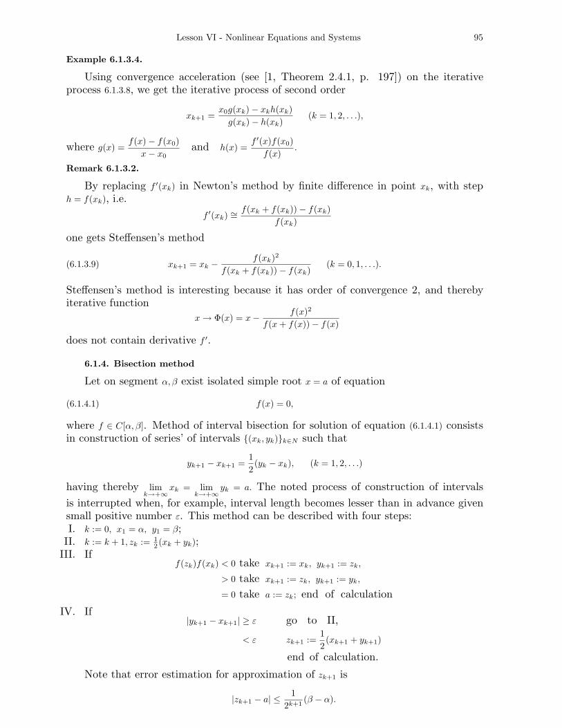
Example 6.1.3.4.
Using convergence acceleration (see [1, Theorem 2.4.1, p. 197]) on the iterativeprocess 6.1.3.8, we get the iterative process of second order
xk+1 =x0g(xk)− xkh(xk)
g(xk)− h(xk)(k = 1, 2, . . .),
where g(x) =f(x)− f(x0)
x− x0and h(x) =
f ′(x)f(x0)f(x)
.
Remark 6.1.3.2.
By replacing f ′(xk) in Newton’s method by finite difference in point xk, with steph = f(xk), i.e.
f ′(xk) ∼=f(xk + f(xk))− f(xk)
f(xk)
one gets Steffensen’s method
(6.1.3.9) xk+1 = xk −f(xk)2
f(xk + f(xk))− f(xk)(k = 0, 1, . . .).
Steffensen’s method is interesting because it has order of convergence 2, and therebyiterative function
x → Φ(x) = x− f(x)2
f(x + f(x))− f(x)
does not contain derivative f ′.
6.1.4. Bisection method
Let on segment α, β exist isolated simple root x = a of equation
(6.1.4.1) f(x) = 0,
where f ∈ C[α, β]. Method of interval bisection for solution of equation (6.1.4.1) consistsin construction of series’ of intervals {(xk, yk)}k∈N such that
yk+1 − xk+1 =12(yk − xk), (k = 1, 2, . . .)
having thereby limk→+∞
xk = limk→+∞
yk = a. The noted process of construction of intervalsis interrupted when, for example, interval length becomes lesser than in advance givensmall positive number ε. This method can be described with four steps:I. k := 0, x1 = α, y1 = β;
II. k := k + 1, zk := 12 (xk + yk);
III. Iff(zk)f(xk) < 0 take xk+1 := xk, yk+1 := zk,
> 0 take xk+1 := zk, yk+1 := yk,
= 0 take a := zk; end of calculation
IV. If|yk+1 − xk+1| ≥ ε go to II,
< ε zk+1 :=12(xk+1 + yk+1)
end of calculation.
Note that error estimation for approximation of zk+1 is
|zk+1 − a| ≤ 12k+1 (β − α).

96 Numerical Methods in Computational Engineering
6.1.5. Schroder Development
Let function f : [α, β] → R be differentiable and f ′(x) 6= 0 (∀x ∈ [α, β]). Consequently, fis then strictly monotonous on [α, β] and there exists its inverse function F which is alsodifferentiable. Then
F ′(y) ==dxdy
=1
f ′(x)(y = f(x)).
If function f is two times differentiable on [α, β] then
F ′′(y) = − f ′′(x)f ′(x)3
.
Finding the higher derivatives of function F , supposing that it is enough times dif-ferentiable, could be very complicated. Being necessary for Schroder development, arecursive procedure is suggested (see [1], pp. 353).
Suppose that function f is (n + 1) times differentiable on [α, β] , and that
(6.1.5.1) F (k)(y) =Xk
(f ′)2k−1 (k = 1, . . . , n + 1),
where Xk is polynomial in f ′, f ′′, . . . , f (k) and f (i) ≡ f (i)(x) for i = 1, . . . , n + 1. By inductionone can prove the formula (6.1.5.1), where polynomial X is determined recursively
(6.1.5.2) Xk+1 = f ′Xk′ − (2k − 1)Xkf ′′,
starting with X1 = 1 and X2 = −f ′′.First five members of series {Xk} are
X1 = 1,
X2 = −f ′′,
X3 = −f ′f ′′′ + 3f ′′2
X4 = −f ′2f IV + 10f ′f ′′f ′′′ − 15f ′′3,
X5 = −f ′3fV + 15f ′2f ′′f IV + 10f ′2f ′′′2 − 105f ′f ′′2f ′′′ + 105f ′′4.
Suppose that function f has on segment [α, β] a simple zero x = a whose surroundingdenote with U(a). If we put h = − f(x)
f ′(x)(x ∈ U(a)), then f(x) + hf ′(x) = 0, wherefrom we
havea = F (0) = F (f + hf ′).
If f ∈ Cn+1[α, β], based on Taylor’s formula we have
a =n
∑
k=0
1k!
F (k)(y)(hf ′)k +F (n+1)(y)(n + 1)!
(hf ′)n+1,
where y = f + thf ′ = (1 − t)f = θf (t, θ ∈ (0, 1)). Finally, using (6.1.5.1) we get Schroderdevelopment
a− x =n
∑
k=1
1k!
Xk
(
f ′
f ′,f ′′
f ′, . . . ,
f (k)
f ′
)
hk + O(f(x)n+1
i.e.
a− x = h− f ′′
2f ′h2 +
3f ′′2 − f ′f ′′′
6f ′2h3(6.1.5.3)
+10f ′f ′′f ′′′ − f ′2f IV − 15f ′′3
24f ′3h4 + . . .

Lesson VI - Nonlinear Equations and Systems 97
6.1.6. Methods of higher order
In this section we will present some ways for obtaining iterative processes with orderof convergence greater than 2, supposing that equation
(6.1.6.1) f(x) = 0,
has on segment [α, β] unique simple root x = a, and that function f is enough timesdifferentiable on [α, β].
1. Using Schroder development, by taking finite number of first members on righthand site of (6.1.5.3), we can get a number of iterative formulas.
LetΦ2(x) = x + h = x− f(x)
f ′(x),
Φ3(x) = Φ2(x)− f(x)′′
2f ′(x)h2 = x− f(x)
f ′(x)− f ′′(x)f(x)2
2f ′(x)3,
Φ4(x) = Φ3(x) +3f ′′2 − f ′f ′′′
6f ′2h3
= x− f(x)f ′(x)
− f ′′(x)f(x)2
2f ′(x)3− f(x)3
6f ′(x)4
(
3f ′′(x)2
f ′(x)− f ′′′(x)
)
,
etc.Note that Φ2(x) is iteration function of Newton’s method.Because h being in first iteration a− x (x → a), based on (6.1.5.3) we have
Φm(x)− a = O(hm) = O((x− a)m) (m = 2, 3, . . .),
when x → a, meaning that
(6.1.6.2) xk+1 = Φm(xk) (k = 0, 1, . . .),
applied to finding root of equation (6.1.6.2), has order of convergence at least m.Formulas (6.1.6.2) are often called Chebyshev iterative formulas.Using Hermite’s interpolation formulas (see Chapter 7) for function f in points
x = xk−1 and x = xk one can get the iterative formula of form (see [10])
(6.1.6.3) xk+1 = xk −f(xk)f ′(xk)
− f(xk)2
2f ′(xk)f′′(xk) (k = 1, 2, . . .),
where f′′(xk) = − 6
ε2k(f(xk)− f(xk−1)) +
2εk
(2f ′(xk) + f ′(xk−1)) and ε = xk − xk−1. Order of con-
vergence of this process is r = 1+√
3. Iterative function of this process is one modificationof Chebyshev function Φ3.
In paper [11], Milovanovic and Petkovic considered one modification of function Φ3
using approximationf ′′(xk) ≈ f ′(xk + εk)− f ′(xk)
εk
whereby ε → 0 when k → +∞. The corresponding iterative process is
(6.1.6.4) xk+1 = xk −f(x)f ′(x)
− f(xk)2
2f ′(xk)3· f ′(xk + εk)− f ′(xk)
εk.
From asymptotic equation (see [1], pp. 357-358)
|ek+1| ∼∣
∣
∣
∣
f ′′′(a)4f ′(a)
∣
∣
∣
∣
|ek|2|ek−1|,
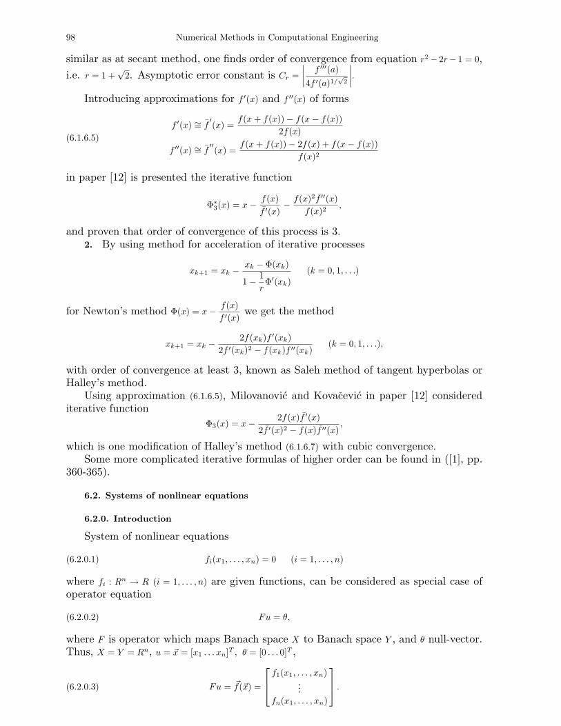
98 Numerical Methods in Computational Engineering
similar as at secant method, one finds order of convergence from equation r2− 2r− 1 = 0,i.e. r = 1 +
√2. Asymptotic error constant is Cr =
∣
∣
∣
∣
f ′′′(a)
4f ′(a)1/√
2
∣
∣
∣
∣
.
Introducing approximations for f ′(x) and f ′′(x) of forms
(6.1.6.5)f ′(x) ∼= f
′(x) =
f(x + f(x))− f(x− f(x))2f(x)
f ′′(x) ∼= f′′(x) =
f(x + f(x))− 2f(x) + f(x− f(x))f(x)2
in paper [12] is presented the iterative function
Φ∗3(x) = x− f(x)f ′(x)
− f(x)2f ′′(x)f(x)2
,
and proven that order of convergence of this process is 3.2. By using method for acceleration of iterative processes
xk+1 = xk −xk − Φ(xk)
1− 1rΦ′(xk)
(k = 0, 1, . . .)
for Newton’s method Φ(x) = x− f(x)f ′(x)
we get the method
xk+1 = xk −2f(xk)f ′(xk)
2f ′(xk)2 − f(xk)f ′′(xk)(k = 0, 1, . . .),
with order of convergence at least 3, known as Saleh method of tangent hyperbolas orHalley’s method.
Using approximation (6.1.6.5), Milovanovic and Kovacevic in paper [12] considerediterative function
Φ3(x) = x− 2f(x)f ′(x)2f ′(x)2 − f(x)f ′′(x)
,
which is one modification of Halley’s method (6.1.6.7) with cubic convergence.Some more complicated iterative formulas of higher order can be found in ([1], pp.
360-365).
6.2. Systems of nonlinear equations
6.2.0. Introduction
System of nonlinear equations
(6.2.0.1) fi(x1, . . . , xn) = 0 (i = 1, . . . , n)
where fi : Rn → R (i = 1, . . . , n) are given functions, can be considered as special case ofoperator equation
(6.2.0.2) Fu = θ,
where F is operator which maps Banach space X to Banach space Y , and θ null-vector.Thus, X = Y = Rn, u = ~x = [x1 . . . xn]T , θ = [0 . . . 0]T ,
(6.2.0.3) Fu = ~f(~x) =
f1(x1, . . . , xn)...
fn(x1, . . . , xn)
.

Lesson VI - Nonlinear Equations and Systems 99
Basic method for solving operator equation (6.2.0.2) and also system of equations (6.2.0.1)is Newton-Kantorowich (Newton-Raphson) method, which is generalization of Newtonmethod (6.1.1.3) .
6.2.1. Newton-Kantorowitch (Raphson) method
Basic iterative method for solving equation (6.2.0.2) is method of Newton-Kantoro-wich, which generalizes classical Newton’s method. Fundamental results regarding ex-istence and uniqueness of solutions of eq. (6.2.0.2) and convergence of the method aregiven by L.V. Kantorowich (see [22]).
Suppose that eq. (6.2.0.2) has a solution u = a and operator F : X → Y is Frechetdifferentiable in convex neighbourhood D of point a. Method of Newton-Kantorowichrely on linearization of eq. (6.2.0.2). Suppose that the approximative solution uk hasbeen found. Then, for obtaining the next approximation uk+1 replace eq. (6.2.0.2) with
(6.2.1.1) Fuk + F ′(uk)(u− uk) = θ.
If for operator F ′(uk) there exists inverse operator Γ(uk) = (F ′(uk))−1, from (6.2.1.1) we obtain
the iterative method
(6.2.1.2) uk+1 = uk − Γ(uk)Fuk (k = 0, 1, . . .)
known as Newton-Kantorowich method. Starting value u0 for generating series {uk} istaken from D, and its selection is very tough problem. Method (6.2.1.2) can be presentedas
uk+1 = Tuk (k = 0, 1, . . .),
whereTu = u− Γ(u)Fu.
For developing a methods for solution of systems of nonlinear equations, we will inducesome crucial theorems without proofs (see [1], pp. 375 - 380].
Theorem 6.2.1.1. Let operator F be two times Frechet differentiable on D, whereby for every u ∈ Dthere exists operator Γ(u). If the operators Γ(u) and F ′′(u) are limited, and u0 ∈ D is close enough topoint a, the iterative process (6.2.1.2) has order of convergence at least two.
For usual consideration we suppose that D is a ball in K[u0, R], where u0 is startingvalue of series {uk}k∈N0 .
If Lipschitz condition
(6.2.1.3) ||F ′(u) − F ′(v)|| ≤ L||u− v|| (u, v ∈ K[u0, R])
is fulfilled, from
Fu− Fv − F ′(v)(u− v) =
1∫
0
[F ′v+t(u−v)) − F ′(v)](u− v)dt
follows the inequality
||Fu− Fv − F ′(v)(u− v)|| ≤ L2
= ||u− v||2.
Theorem 6.2.1.2. Let operator F be Frechet differentiable in the ball K[u0, R] and satisfies the condi-tion (6.2.1.3) and let the nonequalities
(6.2.1.5) ||Γ0|| ≤ b0, ||Γ0Fu0|| ≤ η0, h0 = b0Lη0 ≤12,

100 Numerical Methods in Computational Engineering
where Γ0 = Γ(u0), hold. If
(6.2.1.6) R ≥ r0 =1−
√1− 2h0
h0η0,
series {uk}k∈N0 , generating by means of (6.2.1.2) converges to solution a ∈ K[u0, r0] of equation (6.2.0.2).
For given series’ {bk}, {ηk}, {hk}, {rk} defined with
bk+1 =bk
1− hk, ηk+1 =
hk
2(1− hk)ηk,
hk+1 = bk+1Lηk+1, rk =1−
√
1− 2hk+1
hk+1
the existence of series {uk}k∈N0 is proven and the following relations
(6.2.1.7) ||Γ(uk)|| ≤ bk, ||Γ(uk)Fuk|| ≤ ηk, hk ≤12
and
(6.2.1.8) K[uk, rk] ⊂ K[uk−1, rk−1].
hold.
Theorem 6.2.1.3. When conditions of previous theorem are fulfilled, then it holds
(6.2.1.9) ||uk − a|| ≤ 12k−1 (2h0)2
k−1η0 (k ∈ N).
In order to avoid determination of inverse operator Γ(u) = [F ′(u)]−1 at every step,
method of Newton-Kantorowich can be modified in the following way
(6.2.1.10) uk+1 = uk − Γ0Fuk (k = 0, 1, 2, . . .),
where Γ0 = Γ(u0). By introducing the operator T
(6.2.1.11) Tu = u− Γ0Fu,
the modified method (6.2.1.10) can be given in the form
uk+1 = Tuk (k = 0, 1, 2, . . .).
Suppose that the following conditions are met:a. Operator F is Frechet-differentiable in the ball K[u0, R],b. F ′(u) satisfies the condition (6.2.1.3),c. Operator Γ0 exists and
||Γ0|| ≤ b0, ||Γ0Fu0|| ≤ η0.
Then, it holds the following
Theorem 6.2.1.4. If the following condition hold,
h0 = b0Lη0 <12, and r0 =
1−√
1− 2h0
h0η0 ≤ R
the series generated using (6.2.1.10) converges to solution a ∈ K[u0, r0] of equation (6.2.0.2).
It can be shown that iterative process (6.2.1.10) is of first order.
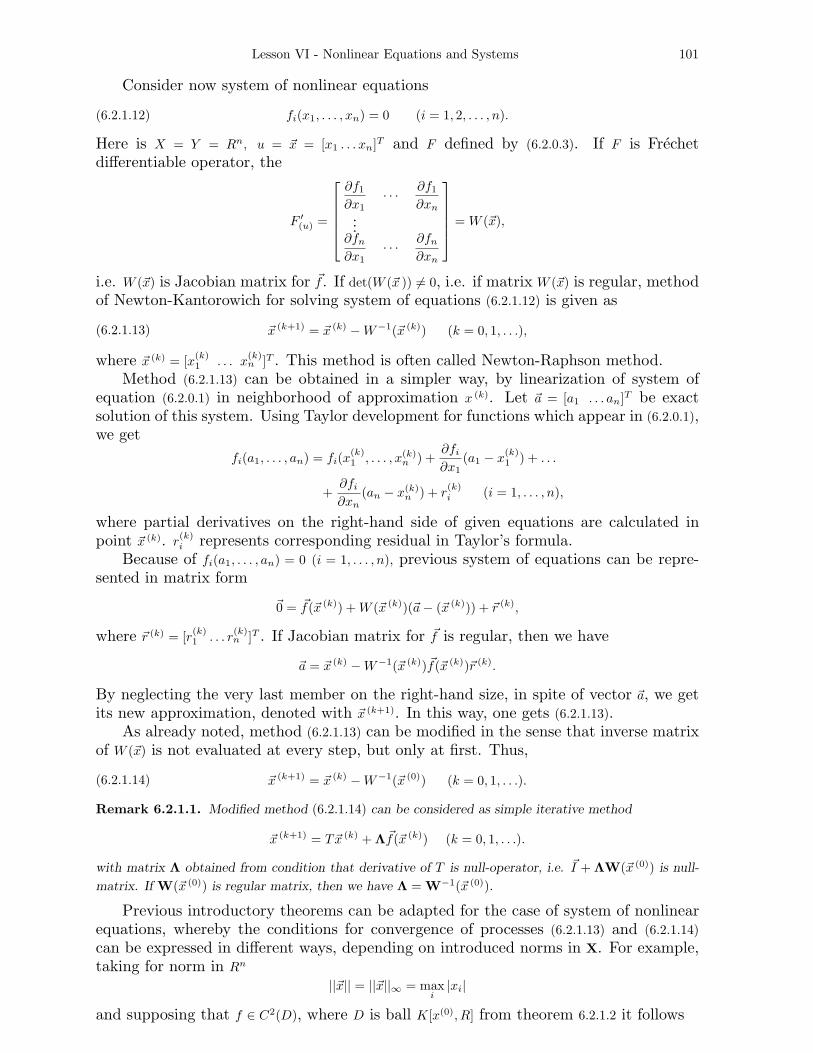
Lesson VI - Nonlinear Equations and Systems 101
Consider now system of nonlinear equations
(6.2.1.12) fi(x1, . . . , xn) = 0 (i = 1, 2, . . . , n).
Here is X = Y = Rn, u = ~x = [x1 . . . xn]T and F defined by (6.2.0.3). If F is Frechetdifferentiable operator, the
F ′(u) =
∂f1
∂x1· · · ∂f1
∂xn...
∂fn
∂x1· · · ∂fn
∂xn
= W (~x),
i.e. W (~x) is Jacobian matrix for ~f . If det(W (~x )) 6= 0, i.e. if matrix W (~x) is regular, methodof Newton-Kantorowich for solving system of equations (6.2.1.12) is given as
(6.2.1.13) ~x (k+1) = ~x (k) −W−1(~x (k)) (k = 0, 1, . . .),
where ~x (k) = [x(k)1 . . . x(k)
n ]T . This method is often called Newton-Raphson method.Method (6.2.1.13) can be obtained in a simpler way, by linearization of system of
equation (6.2.0.1) in neighborhood of approximation x (k). Let ~a = [a1 . . . an]T be exactsolution of this system. Using Taylor development for functions which appear in (6.2.0.1),we get
fi(a1, . . . , an) = fi(x(k)1 , . . . , x(k)
n ) +∂fi
∂x1(a1 − x(k)
1 ) + . . .
+∂fi
∂xn(an − x(k)
n ) + r(k)i (i = 1, . . . , n),
where partial derivatives on the right-hand side of given equations are calculated inpoint ~x (k). r(k)
i represents corresponding residual in Taylor’s formula.Because of fi(a1, . . . , an) = 0 (i = 1, . . . , n), previous system of equations can be repre-
sented in matrix form
~0 = ~f(~x (k)) + W (~x (k))(~a− (~x (k))) + ~r (k),
where ~r (k) = [r(k)1 . . . r(k)
n ]T . If Jacobian matrix for ~f is regular, then we have
~a = ~x (k) −W−1(~x (k))~f(~x (k))~r (k).
By neglecting the very last member on the right-hand size, in spite of vector ~a, we getits new approximation, denoted with ~x (k+1). In this way, one gets (6.2.1.13).
As already noted, method (6.2.1.13) can be modified in the sense that inverse matrixof W (~x) is not evaluated at every step, but only at first. Thus,
(6.2.1.14) ~x (k+1) = ~x (k) −W−1(~x (0)) (k = 0, 1, . . .).
Remark 6.2.1.1. Modified method (6.2.1.14) can be considered as simple iterative method
~x (k+1) = T~x (k) + Λ~f(~x (k)) (k = 0, 1, . . .).
with matrix Λ obtained from condition that derivative of T is null-operator, i.e. ~I + ΛW(~x (0)) is null-matrix. If W(~x (0)) is regular matrix, then we have Λ = W−1(~x (0)).
Previous introductory theorems can be adapted for the case of system of nonlinearequations, whereby the conditions for convergence of processes (6.2.1.13) and (6.2.1.14)can be expressed in different ways, depending on introduced norms in X. For example,taking for norm in Rn
||~x|| = ||~x||∞ = maxi|xi|
and supposing that f ∈ C2(D), where D is ball K[x(0), R] from theorem 6.2.1.2 it follows

102 Numerical Methods in Computational Engineering
Corollary 6.2.1.1. If in D are fulfilled the following conditions:
(6.2.1.15) sij =n
∑
k=1
∣
∣
∣
∣
∂2fi
∂xj∂xk
∣
∣
∣
∣
(i, j = 1, . . . , n);
(6.2.1.16) ||~f(~x(0)
)|| ≤ Q, ||W−1(~x(0)
)|| ≤ b;
(6.2.1.17) ∆0 = detW(~x(0)
) 6= 0, h = nNQb2 ≤ 12.
Then, if R ≥ r =1−
√1− 2hh
Qb, method Newton-Kantorowich (6.2.1.13) converges to solution a ∈
K[~x(0)
, r].
Because for 0 < h ≤ 1/2 it holds (1 −√
1− 2h)/h ≤ 2, so that for r in Corollary 6.2.1.1we can take r = 2Qb.
Modified Newton-Kantorowich method (6.2.1.14) converges also under conditionsgiven in Corollary 6.2.1.1.
In [1, pp. 384-386] the Newton-Kantorowich method is illustrated with system ofnonlinear equation in two unknowns. It is suggested to reader to write a program codein Mathematica and Fortran.
Example 6.2.1.1. Solve the system of nonlinear equation
f1(x1, x2) = 9x21x2 + 4x2
2 − 36 = 0
f2(x1, x2) = 16x22 − x4
1 + x2 + 1 = 0,
which has a solution in first quadrant (x1, x2 > 0).
Using graphic presentation of implicit functions f1 and f2 in first quadrant, one cansee that solution ~a is located in the neighborhood of point (2, 1), so that we take forinitial vector ~x(0) = [2 1]T , i.e. x(0)
1 = 2 and x(0)2 = 1.
By partial derivation of f1 and f2 one gets the Jacobian
W (x) =[
18x1x2 9x21 + 8x2
−4x31 32x2 + 1
]
,
and its inverseW−1(~x) =
1∆(~x )
[
32x2 + 1 −(9x21 + 8x2)
4x31 18x1x2
]
,
where∆(~x) = 18x1x2(32x2 + 1) + 4x3
1(9x21 + 8x2).
By putting f (k)i ≡ fi(x
(k)1 , x(k)
2 ) and ∆k ≡ ∆(x(k)) (i = 1, 2; k = 0, 1 . . .) in the scalar form ofNewton-Kantorowich formula (6.2.1.13), we get the iteration formula
x(k+1)1 = x(k)
1 − 1∆k
{(32x(k)2 + 1)f (k)
1 − (9x(k)2
1 + 8x(k)2 )f (k)
2 },
x(k+1)2 = x(k)
2 − 1∆k
{4x(k)3
1 f (k)1 + 18x(k)
1 x(k)2 f (k)
2 }.
The appropriate Fortran code for solving given nonlinear equation isDouble precision x1,x2,x10,x11,x20,x21,f1,f2,Delta,EPSF1(x1,x2)=9*x1**2*x2 + 4*x2**2-36F2(x1,x2)=16*x2**2 - x1**4 + x2 + 1Delta(x1,x2)=18*x1*x2*(32*x2+1)+4*x1**3*(9*x1**2+8*x2)

Lesson VI - Nonlinear Equations and Systems 103
Open(1, File=’Newt-Kant.out’)x10=2.d0x20=1.d0EPS=1.d-6Iter=0write(1,5)
5 format(1h ,// 3x, ’i’,7x,’x1(i)’,9x,’x2(i)’,* 9x,’f1(i)’, 9x,’f2(i)’/)write(1,10)Iter, x10,x20,F1(x10,x20),F2(x10,x20)
1 x11=x10-((32*x20+1)*f1(x10,x20)-(9*x10**2+8*x20)** f2(x10,x20)) /Delta(x10,x20)x21=x20-(4*x10**3*f1(x10,x20)+18*x10*x20*f2(x10,x20))
* /Delta(x10,x20)Iter=Iter+1write(1,10)Iter, x11,x21,F1(x11,x21),F2(x11,x21)
10 Format(1x,i3, 4D14.8,2x)If(Dabs(x10-x11).lt.EPS.and.Dabs(x20-x21).lt.EPS)stopIf(Iter.gt.100)Stopx10=x11x20=x21go to 1End
and the output list of results isi x1(i) x2(i) f1(i) f2(i)0 .20000000D+01 .10000000D+01 .40000000D+01 .20000000D+011 .19830508D+01 .92295840D+00 .73136345D-01 .88110835D-012 .19837071D+01 .92074322D+00-.28694053D-04 .68348441D-043 .19837087D+01 .92074264D+00-.10324186D-10-.56994853D-104 .19837087D+01 .92074264D+00 .00000000D+00-.15543122D-14
6.2.2. Gradient method
Because Newton-Kantorowich method demands obtaining inverse operator F ′−1(u),
what can be very complicated, and even impossible, it have been developed a wholeclass of quasi-Newton methods, which use some approximations of noted operator (see[21], [22], [23], [24]). One of this methods is gradient method.
For given system of nonlinear equations (6.2.1.12), with matrix form (see (6.2.0.3))
(6.2.2.1) ~f(~x) = ~0.
The gradient method for solving a given system of equations is based on minimizationof functional
U(~x) =n
∑
i=1
fi(x1, . . . , xn)2 = (~f(~x), ~f(~x)).
It is easy to show that the equivalence U(~x) = 0 ⇐⇒ ~f(~x) = ~0 holds.Suppose that equation (6.2.2.1) has unique solution ~x = ~a, for which functional U riches
minimum value. Let ~x(0) be initial approximation of this solution. Let us construct series{~x(k)} such that U(~x(0)) > U(~x(1)) > U(~x(2)) > · · ·. In a same way as at linear equations (seeChap. IV), we take
(6.2.2.2) ~x (k+1) = ~x (k) − λk∇U(~x (k)) (k = 0, 1, . . .),
where ∇U(~x) = grad(~x) =[
∂U∂x1
· · · ∂U∂xn
]T
. Parameter λk is to be determined from condition
that scalar function S, defined with S(t) = U(~x (k) − t∇U(~x (k))) has a minimum value inpoint t = λk. Having in mind that equation S′(t) = 0 is non-linear, proceed its linearizationaround t = 0. In this case we have
L(k)i = fi(~x (k) − t∇U(~x (k))) = fi(~x (k))− t(∇fi(~x (k)),∇U(~x (k)))

104 Numerical Methods in Computational Engineering
so that linearized equation is
n∑
i=1
L(k)i
ddt
L(k)i = −
n∑
i=1
L(k)i (∇fi~x (k)),∇U(~x (k))) = 0,
wherefrom we obtain
(6.2.2.3) λk = t =
n∑
i=1Hifi(~x (k))
n∑
i=1H2
i
,
where we put Hi = (∇fi(~x (k)), ∇U(~x (k))) (i = 1, . . . , n). Because of
∂U∂xj
=∂
∂xj
{ n∑
i=1
fi(~x )2}
= 2n
∑
i=1
fi(~x )∂fi(~x )
∂xj,
we have
(6.2.2.4) ∇U(~x ) = 2WT (~x )~f(~x ),
where W(~x ) is Jacobian matrix.According to previous, (6.2.2.3) reduces to
λk =12· (~f (k),WkWT
k~f (k))
(WkWTk
~f (k),WkWTk
~f (k)),
where ~f (k) = ~f(~x (k)) and Wk = W(~x (k)). Finally, gradient method can be represented inthe form
~x (k+1) = ~x (k) − 2λkWTk
~f(~x (k)) (k = 0, 1, . . .).
As we see, in spite of matrix W−1(~x (k)) which appears in Newton-Kantorowichmethod, we have now matrix 2λkWT
k .
Example 6.2.1.2. System of nonlinear equations given in example 6.2.1.1 will be solved using gradientmethod, starting with the same initial vector ~x(0) = [2 1]T , giving the following list of results
i x1(i) x2(i) 2lam_k0 .2000000000D+01 .1000000000D+01 .305787395D-031 .1975537008D+01 .9259994504D+00 .538747689D-032 .1983210179D+01 .9201871306D+00 .339553623D-033 .1983643559D+01 .9207840032D+00 .535596539D-034 .1983705230D+01 .9207387845D+00 .339328604D-035 .1983708270D+01 .9207429317D+00 .535573354D-036 .1983708709D+01 .9207426096D+00 .393325162D-037 .1983708731D+01 .9207426391D+00 .535990624D-038 .1983708234D+01 .9207429368D+00 .337793301D-039 .1983708734D+01 .9207426370D+00
Note that the convergence here is much slower than at Newton-Kantorowich method,due to fact that gradient method is of first order.
Gradient method is successfully used in many optimization problems of nonlinearprogramming, with large number of methods, especially of gradient type, which are basisfor number of programming packages for solving nonlinear programming problems.
6.2.3. Globally convergent methods
We have seen that Newtons method and Newton-like methods (quasi-Newton meth-ods) for solving nonlinear equations has an unfortunate tendency not to converge if theinitial guess is not sufficiently close to the root. A global method is one that converges

Lesson VI - Nonlinear Equations and Systems 105
to a solution from almost any starting point. Therefore, it is our goal to develop analgorithm that combines the rapid local convergence of Newtons method with a glob-ally convergent strategy that will guarantee some progress towards the solution at eachiteration. The algorithm is closely related to the quasi-Newton method of minimization(see [5], p. 376).
From (6.2.1.13), Newton-Raphson method, we have so known Newton step in iterationformula
(6.2.3.1) ~x (k+1) − ~x (k) = δ~x = −W−1(~x (k))~f(~x (k)), (k = 0, 1, . . .)
where W is Jacobian matrix. The question is how one should decide to accept theNewton step δx? If we denote F = ~f(~x (k)), a reasonable strategy for step acceptance isthat |F|2 = F · F decreases, what is the same requirement one would impose if trying tominimize
(6.2.3.2) f =12F · F.
Every solution of (6.2.1.12) minimizes (6.2.3.2), but there may be some local minima of(6.2.3.2) that are not solution of (6.2.1.12). Thus, simply applying some minimum findingalgorithms can be wrong.
To develop a better strategy, note that Newton step (6.2.3.1) is a descent directionfor f :
(6.2.3.3) ∇f · δ~x = (F ·W) · (−W−1 · F) = −F · F < 0.
Thus, the strategy is quite simple. One should first try the full Newton step, becauseonce we are close enough to the solution, we will get quadratic convergence. However,we should check at each iteration that the proposed step reduces f . If not, we goback (backtrack) along the Newton direction until we get acceptable step. Because theNewton direction is descent direction for f , we fill find for sure an acceptable step bybacktracking.
It is to mention that this strategy essentially minimizes f by by taking Newton stepsdetermined in such a way that bring ∇f to zero. In spite of fact that this method canoccasionally lead to local minimum of f , this is rather rare in practice. In such a case,one should try a new starting point.
Line Searches and Backtracking
When we are not close enough to the minimum of f , taking the full Newton step ~p =δ~x need not decrease the function; we may move too far for the quadratic approximationto be valid. All we are guaranteed is that initially f decreases as we move in the Newtondirection. So the goal is to move to a new point xnew along the direction of the Newtonstep ~p, but not necessarily all the way (see [5], pp. 377-378):
(6.2.3.4) ~xnew = ~xold + λ~p (0 < λ ≤ 1)
The aim is to find λ so that f(~xold + λ~p) has decreased sufficiently. Until the early 1970s,standard practice was to choose λ so that ~xnew exactly minimizes f in the direction ~p.However, we now know that it is extremely wasteful of function evaluations to do so. Abetter strategy is as follows: Since ~p is always the Newton direction in our algorithms,we first try λ = 1, the full Newton step. This will lead to quadratic convergence when~x is sufficiently close to the solution. However, if f(~xnew) does not meet our acceptancecriteria, we backtrack along the Newton direction, trying a smaller value of λ, until

106 Numerical Methods in Computational Engineering
we find a suitable point. Since the Newton direction is a descent direction, we areguaranteed to decrease f for sufficiently small λ. What should the criterion for acceptinga step be? It is not sufficient to require merely that f(~xnew) < f(~xold). This criterion canfail to converge to a minimum of f in one of two ways. First, it is possible to constructa sequence of steps satisfying this criterion with f decreasing too slowly relative to thestep lengths. Second, one can have a sequence where the step lengths are too smallrelative to the initial rate of decrease of f . A simple way to fix the first problem is torequire the average rate of decrease of f to be at least some fraction α of the initial rateof decrease ∇f · ~p
(6.2.3.5) f(~xnew) ≤ f(~xold) + α∇f · (~xnew − ~xold).
Here the parameter α satisfies 0 < α < 1. We can get away with quite small values ofα; α = 10−4 is a good choice. The second problem can be fixed by requiring the rate ofdecrease of f at ~xnew to be greater than some fraction β of the rate of decrease of f at ~xold.In practice, we will not need to impose this second constraint because our backtrackingalgorithm will have a built-in cutoff to avoid taking steps that are too small.
Here is the strategy for a practical backtracking routine. Define
(6.2.3.6) g(λ) ≡ f(~xold + λ~p)
so that
(6.2.3.7) g′(λ) = ∇f · ~p
If we need to backtrack, then we model g with the most current information we haveand choose λ to minimize the model. We start with g(0) and g′(0) available. The firststep is always the Newton step, λ = 1. If this step is not acceptable, we have availableg(1) as well. We can therefore model g(λ) as a quadratic:
(6.2.3.8) g(λ) ≈ [g(1)− g(0)− g′(0)]λ2 + g(0).
By first derivative of this function we find the minimum condition
(6.2.3.9) λ = − g′(0)2[g(1)− g(0)− g′(0)]
.
Since the Newton step failed, we can show that λ<∼
12 for small α. We need to guard
against too small a value of λ, however. We set λmin = 0.1.On second and subsequent backtracks, we model g as a cubic in λ, using the previous
value g(λ1) and the second most recent value g(λ2).
(6.2.3.10) g(λ) = aλ3 + bλ2 + g′(0)λ + g(0)
Requiring this expression to give the correct values of g at λ1 and λ2 gives twoequations that can be solved for the coefficients a and b.
(6.2.3.11)[
ab
]
=1
λ1 − λ2
[
1/λ21 −1/λ2
2−λ2/λ2
1 λ1/λ22
]
·[
g(λ1)− g′(0)λ1 − g(0)g(λ2)− g′(0)λ2 − g(0)
]
.
The minimum of the cubic (6.2.3.10) is at
(6.2.3.12) λ =−b +
√
b2 − 3ag′(0)3a
.

Lesson VI - Nonlinear Equations and Systems 107
One should enforce that λ lie between λmax = 0.5λ1 and λmin = 0.1λ1. The correspondingcode in FORTRAN is given in [5], pp. 378-381. It it suggested to reader to write thecorresponding code in Mathematica.
Multidimensional Secant Methods: Broyden’s Method
Newton’s method as used previously is rather efficient, but it still have several dis-advantages. One of the most important is that it needs Jacobian matrix. In manyproblems the Jacobian matrix is not available, i.e. there do not exist analytic deriva-tives. If the function evaluation is complicated, the finite-difference determination ofJacobian can be prohibitive. There are quasi-Newton methods which provide cheapapproximation to the Jacobian for the purpose of zero finding. The methods are oftencalled secant methods, because they reduce in one dimension to the secant method. Oneof the best of those methods is Broyden’s method (see [21]).
If one denotes approximate Jacobian by B, then the i-th quasi-Newton step δ~xi isthe solution of
(6.2.3.13) Bi · δ~xi = −Fi,
where δ~xi = ~xi+1 − ~xi. Quasi-Newton or secant condition is that Bi+1 satisfy
(6.2.3.14) Bi+1 · δ~xi = δFi,
where δFi = Fi+1−Fi. This is generalization of the one-dimensional secant approximationto the derivative, δF/δx. However, equation (6.2.3.14) does not determine Bi+1 uniquelyin more than one dimension. Many different auxiliary conditions to determine Bi+1 havebeen examined, but the best one results from the Broyden’s formula. This formula isbased on idea of getting Bi+1 by making a least change to Bi in accordance to the secantequation (6.2.3.14). Broyden gave the formula
(6.2.3.15) Bi+1 = Bi +(δFi −Bi · δ~xi)⊗ δ~xi
δ~xi · δ~xi.
One can check that Bi+1 satisfies (6.2.3.14).Early implementations of Broyden’s method used the Sherman-Morrison formula to
invert equation analytically,
(6.2.3.16) B−1i+1 = B(−1)
i +(δ~xi −B−1
i · δFi)⊗ δ~xi ·B−1i
δ~xi · δB−1i · δFi
.
Thus, instead of solving equation (6.2.3.1) by, for example, LU decomposition, one de-termined
(6.2.3.17) δ~xi = −B−1i · Fi
by matrix multiplication in O(n2) operations. The disadvantage of this method is thatit cannot be easily embedded in a globally convergent strategy, for which the gradientof equation (6.2.3.2) requires B, not B−1
(6.2.3.18) ∇(12F · F) ' BT · F
Accordingly, one should implement the update formula in the form (6.2.3.15). However,we can still preserve the O(n2) solution of (6.2.3.1) by using QR decomposition of Bi+1
in O(n2) operations. All needed is initial approximation B0 to start process. It is oftenaccepted to take identity matrix, and then allow O(n) updates to produce a reasonable

108 Numerical Methods in Computational Engineering
approximation to the Jacobian. In [5], p. 382-383, the first n function evaluations arespent on a finite-difference approximation in order to initialize B. Since B is not exactJacobian, it is not guaranteed that δ~x is descent direction for f = 1
2F ·F (see eq. (6.2.3.3)).That has a consequence that the line search algorithm can fail to return the suitablestep if B is far from the true Jacobian. In this case we simply reinitialize B.
Like the secant method in one dimension, Broyden’s method converges superlinearlyonce you get close enough to the root. Embedded in a global strategy, it is almost asrobust as Newton’s method, and often needs far fewer function evaluations to determinea zero. Note that the final value of B is not always close to the true Jacobian at theroot, in spite of fact that method converges.
The programme code ([5], pp. 383-385) of Broyden’s method differs from Newtonianmethods in using QR decomposition instead of LU, and determination of Jacobian byfinite-difference approximation instead of direct evaluation.
More Advanced Implementations
One of the principal ways that the methods described above can fail is if matrix W(Newton-Kantorowich) or B (Broyden’s method) becomes singular or nearly singular,so that ∆x cannot be determined. This situation will not occur very often in practice.Methods developed so far to deal with this problem involve the monitoring of conditionnumber of W and perturbing W if singularity or near singularity is detected. Thisfeature is most easily implemented if QR decomposition instead of LU decompositionin Newton (or quasi-Newton) method is applied. However, in spite of fact that thismethod can solve problems when W is exactly singular and Newton’s and Newton-likemethods fail, it is occasionally less robust on other problems where LU decompositionsucceeds. Implementation details, like roundoff, underflow, etc. are to be consideredand taken in account.
In [5], considering effectiveness of strategies for minimization and zero finding, theglobal strategies have been based on line searches. Other global algorithms, like hookstep and dogleg step methods, are based on the model-trust region approach, which isrelated to the Levenberg-Marquardt algorithm for nonlinear least-squares. In spite beingmore complicated than line searches, these methods have a reputation for robustnesseven when starting far from desired zero or minimum.
Numerous libraries and software packages are available for solving nonlinear equa-tions. Many workstations and mainframe computers have such libraries attached tooperating systems. Many commercial software packages contain nonlinear equationsolvers. Very popolar among engineers are Matlab and Matcad. More sophisticatedpackages like Mathematica, IMSL, Macsyma, and Maple contain programs for nonlin-ear equation solving. The book Numerical recipes [5] contains numerous programs forsolving nonlinear equation.
Bibliography (Cited references and further reading)
[1] Milovanovic, G.V., Numerical Analysis I, Naucna knjiga, Beograd, 1988 (Serbian).[2] Hoffman, J.D., Numerical Methods for Engineers and Scientists. Taylor & Francis,
Boca Raton-London-New York-Singapore, 2001.[3] Milovanovic, G.V. and Djordjevic, Dj.R., Programiranje numerickih metoda na
FORTRAN jeziku. Institut za dokumentaciju zastite na radu ”Edvard Kardelj”,Nis, 1981 (Serbian).
[4] Stoer, J., and Bulirsch, R., Introduction to Numerical Analysis, Springer, New York,1980.
[5] Press, W.H., Flannery, B.P., Teukolsky, S.A., and Vetterling, W.T., Numerical Re-cepies - The Art of Scientific Computing. Cambridge University Press, 1989.

Lesson VI - Nonlinear Equations and Systems 109
[6] Djordjevic, L.N., An iterative solution of algebraic equations with a parameter toaccelerate convergence. Univ. Beograd. Publ. Elektrotehn. Fak. Ser. Mat.Fiz. No.412- No. 460(1973), 179-182.
[7] Tihonov, O.N., O bystrom vychyslnii najbolshih kornei mnogoclena. Zap. Leningrad.gorn. in-ta 48, 3(1968), 36-41.
[8] Ostrowski, A., Solution of Equations and System of Equations. Academic Press,New Yurk, 1966.
[9] Wegstein, J.H., Accelerating convergence of iterative processes. Comm. ACM 1(1958), 9-13.
[10] Ralston,A., A First Course in Numerical Analysis.McGraw-Hill, New York, 1965.
[11] Milovanovic, G.V. & Petkovic, M.S., On some modifications of a third order methodfor solving equations. Univ. Beograd. Publ. Elektroteh. Fak. Ser. Mat. Fiz. No. 678- No. 715 (1980), pp. 63-67.
[12] Milovanovic, Kovacevic, M.A., Two iterative processes of third order without deriva-tives. IV Znanstveni skup PPPR, Stubicke Toplice, 1982, Proceedings, pp. 63-67(Serbian).
[13] Varjuhin, V.A. and Kasjanjuk, S.A., Ob iteracionnyh metodah utocnenija korneiuravnenii. Z. Vychysl. Mat. i Mat. Fiz. 9(1969), 684-687.
[14] Lika, D.K., Ob iteracionnyh metodah vissego porjadka. Dokl. 2-i Nauc.-tehn. respubl.konf. Moldavii. Kishinev, 1965, pp.13-16.
[15] Djordjevic, L.N. & Milovanovic, G.V., A combined iterative formula for solving equa-tions. Informatika 78, Bled 1978, 3(207).
[16] Petkovic, M.S., Some iterative interval methods for solving equations. Ph.D. thesis,University Nis, 1980.
[17] Petkovic, M.S. & Petkovic, D. Lj., On a method for two-sided approaching for solvingequations. Freiburger Intervall-Berichte 10(1980), pp. 1-10.
[18] Hoffman, J.D., Numerical Methods for Engineers and Scientists. Taylor & Francis,Boca Raton-London-New York-Singapore, 2001.
[19] IMSL Math/Library Users Manual , IMSL Inc., 2500 City West Boulevard, HoustonTX 77042
[20] NAG Fortran Library, Numerical Algorithms Group, 256 Banbury Road, OxfordOX27DE, U.K., Chapter F02.
[21] Broyden, C.G., Quasi-Newton methods and their application to function minimiza-tion, Math. Comp. 29(1967), 368-381.
[22] Kantorowich, L.V., Funkcional’nyi analiz i prikladnaja matematika., Uspehi Mat.Nauk 3(1948), 89-185.
[23] Ortega, J.M. & Rheinboldt, W.C., Iterative solution of nonlinear equations in severalvariables, Academic Press, New York, 1970.
[24] Rall, L., Computational solution of nonlinear operator equations, New York, 1969.[25] Kul’cickii, O.Ju. & Simelevic, L.I., O nahozdenii nacal’nogo pribizenija., Z. Vycisl.
Mat. i Mat. Fiz. 14(1974), pp. 1016-1018.[26] Dennis, J.E. and Schnabel, R.B., Numerical Methods for Unconstrained Optimiza-
tion and Nonlinear Equations, Englewood Cliffs, NJ: Prentice Hall, 1983.