6.002x circuits and electronics · pdf filemotivating example – slow case our old...
TRANSCRIPT
1
Second-Order Systems
6.002x CIRCUITS AND ELECTRONICS
[Review complex algebra Appendix C in textbook]
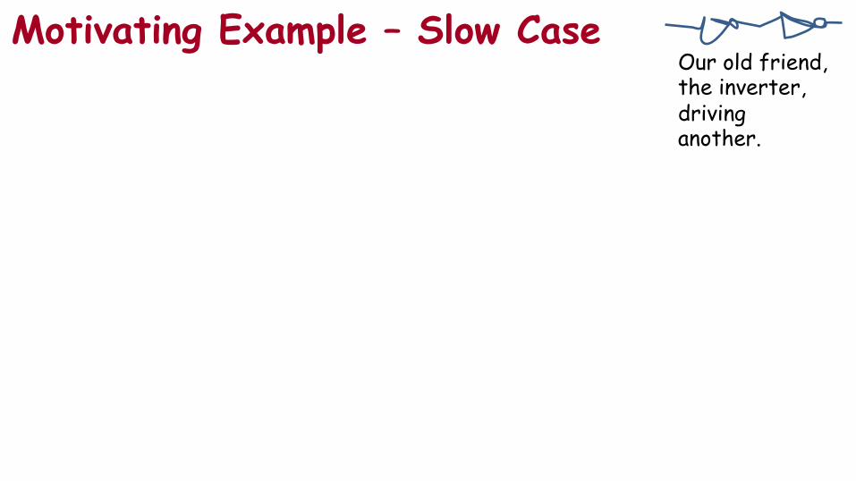
Motivating Example – Slow Case Our old friend, the inverter, driving another.

3
Observed Output - Slow
vA
5
0
vB
0
vC
0 t
t
t
C A B
5V
+!–!
5V
CGS
2KΩ 2KΩ
5
5
Demo
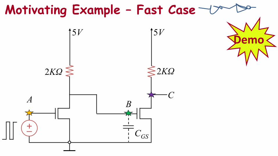
Motivating Example – Fast Case
C A B
5V
+!–!
5V
CGS
2KΩ 2KΩ
Demo

5
Observed Output – Fast Case
vA
5
0
vB
0
vC
0 t
t
t
C A B
5V
+!–!
5V
CGS
2KΩ 50Ω
2KΩ S
5
5

Fast Case – What’s Really Going On
C A B
5V
+!–!
5V
CGS
2KΩ 50Ω
2KΩ S

Second-Order Systems
+!–!5V CGS
2KΩ B
L
Relevant circuit: C A B
5V
+!–!
5V
CGS
large loop
2KΩ 50Ω
2KΩ S
L

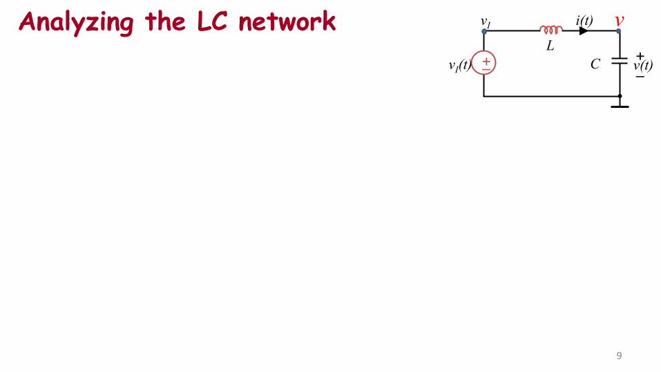
First, let’s analyze the LC network
9
Analyzing the LC network +!–! C
L +!–!v(t)
i(t) v
vI(t)
vI

10
Solving

11
Let’s solve

12
1 Particular solution

13
1 Particular solution
IPP Vv
dtvdLC =+2
2

14
Homogeneous solution 2

15
02
2
=+ HH v
dtvdLCSolution to
Homogeneous solution 2
Recall, vH : solution to homogeneous equation (drive set to zero)
Four-step method:
Assume solution of the form* 2A ?s,A,Aev st
H ==*Differential equations are commonly solved by guessing solutions

16
02
2
=+ HH v
dtvdLCHomogeneous solution 2

17
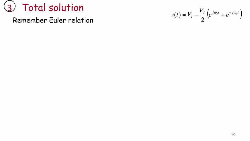
Total solution 3

18
Total solution 3 Find unknowns from initial conditions.
tjtjI
oo eAeAVtv ωω −++= 21)(v(t) = vP(t) = vH (t)
19
Remember Euler relation Total solution 3 ( )tjtjI
Ioo eeVVtv ωω −+−=
2)(

20
Plotting the Total Solution
0 0
v(t) i(t)
tVVtv oII ωcos)( −=
Demo

21
Summary of Method Write DE for circuit by applying node method.
Find particular solution vP by guessing and trial & error.
Find homogeneous solution vH
Total solution is vP + vH , then solve for remaining constants using initial conditions.
Assume solution of the form Aest .
Obtain characteristic equation.
Solve characteristic equation for roots si .
Form vH by summing Ai esit terms.
1
2 3
4
D
C
A
B

22
What if we have:
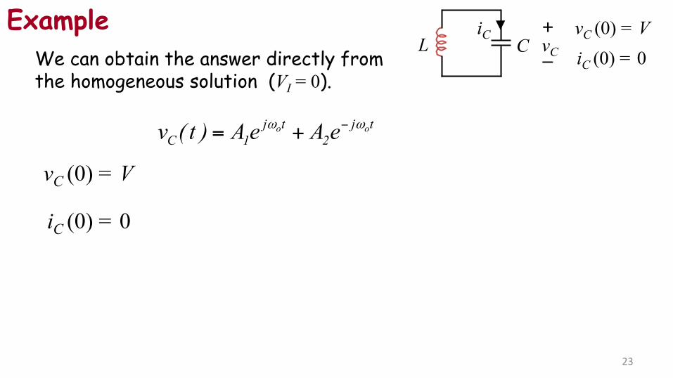
Example
23
We can obtain the answer directly from the homogeneous solution (VI = 0).
tj2
tj1C
oo eAeA)t(v ωω −+=
Example C L
+!
–!iC
vC
vC (0) = V
iC (0) = 0
vC (0) = V
iC (0) = 0

24
Example
π2
iC
π2
vc V

25
Energy
toωπ2
EC
toωπ2
EL

26
Next, introduce R: RLC Circuits
More in the next sequence! If you are impatient, see A&L Section 13.2
+!–! C
L
+!
–!vI (t)
i(t)
v(t)
v(t)
t