6254 ieee transactions on signal processing, …people.oregonstate.edu/~fuxia/tsp_rvolmin.pdf ·...
TRANSCRIPT

6254 IEEE TRANSACTIONS ON SIGNAL PROCESSING, VOL. 64, NO. 23, DECEMBER 1, 2016
Robust Volume Minimization-Based MatrixFactorization for Remote Sensing
and Document ClusteringXiao Fu, Member, IEEE, Kejun Huang, Student Member, IEEE, Bo Yang, Student Member, IEEE,
Wing-Kin Ma, Senior Member, IEEE, and Nicholas D. Sidiropoulos, Fellow, IEEE
Abstract—This paper considers volume minimization (VolMin)-based structured matrix factorization. VolMin is a factorizationcriterion that decomposes a given data matrix into a basis matrixtimes a structured coefficient matrix via finding the minimum-volume simplex that encloses all the columns of the data matrix.Recent work showed that VolMin guarantees the identifiability ofthe factor matrices under mild conditions that are realistic in a widevariety of applications. This paper focuses on both theoretical andpractical aspects of VolMin. On the theory side, exact equivalenceof two independently developed sufficient conditions for VolMinidentifiability is proven here, thereby providing a more compre-hensive understanding of this aspect of VolMin. On the algorithmside, computational complexity and sensitivity to outliers are twokey challenges associated with real-world applications of VolMin.These are addressed here via a new VolMin algorithm that han-dles volume regularization in a computationally simple way, andautomatically detects and iteratively downweights outliers, simul-taneously. Simulations and real-data experiments using a remotelysensed hyperspectral image and the Reuters document corpus areemployed to showcase the effectiveness of the proposed algorithm.
Index Terms—Document clustering, hyperspectral unmixing,identifiability, matrix factorization, robustness against outliers,simplex-volume minimization (VolMin).
I. INTRODUCTION
S TRUCTURED MATRIX FACTORIZATION (SMF) hasbeen a popular tool in signal processing and machine learn-
ing. For decades, factorization models such as the singular valuedecomposition (SVD) and eigen-decomposition have been ap-plied for dimensionality reduction (DR), subspace estimation,noise suppression, feature extraction, etc. Motivated by the in-fluential paper of Lee and Seung [2], new SMF models suchas nonnegative matrix factorization (NMF) have drawn much
Manuscript received March 3, 2016; revised June 8, 2016 and July 28, 2016;accepted August 6, 2016. Date of publication August 25, 2016; date of currentversion October 6, 2016. The associate editor coordinating the review of thismanuscript and approving it for publication was Prof. Wee Peng Tay. Thiswork was supported in part by the National Scientific Foundation (NSF) underProject NSF-ECCS 1608961 and in part by the Hong Kong Research GrantsCouncil under Project CUHK 14205414. A part of this work was presented inthe Proceedings of the IEEE International Conference on Acoustics, Speech,and Signal Processing 2016 [1].
X. Fu, K. Huang, B. Yang, and N. D. Sidiropoulos are with the De-partment of Electrical and Computer Engineering, University of Minnesota,Minneapolis, MN 55455, USA (e-mail: [email protected]; [email protected];[email protected]; [email protected]).
W.-K. Ma is with the Department of Electronic Engineering, TheChinese University of Hong Kong, Shatin, N.T., Hong Kong (e-mail:[email protected]).
Color versions of one or more of the figures in this paper are available onlineat http://ieeexplore.ieee.org.
Digital Object Identifier 10.1109/TSP.2016.2602800
attention, since they are capable of not only reducing dimension-ality of the collected data, but also retrieving loading factors thathave physically meaningful interpretations.
In addition to NMF, some related SMF models have attractedconsiderable interest in recent years. The remote sensing com-munity has spent much effort on a class of factorizations wherethe columns of one factor matrix are constrained to lie in theunit simplex [3]. The same SMF model has also been utilized fordocument clustering [4], and, most recently, multi-sensor arrayprocessing and blind separation of power spectra for dynamicspectrum access [5], [6].
The first key question concerning SMF lies in identifiability–when does a factorization model or criterion admit unique so-lution in terms of its factors? Identifiability is important inapplications such as parameter estimation, feature extraction,and signal separation. In recent years, identifiability conditionshave been investigated for the NMF model [7]–[9]. An unde-sirable property of NMF highlighted in [9] is that identifiabilityhinges on both loading factors containing a certain number ofzeros. In many applications, however, there is at least one factorthat is dense. In hyperspectral unmixing (HU), for example, thebasis factor (i.e., the spectral signature matrix) is always dense.On the other hand, very recent work [5], [10] showed that theSMF model with the coefficient matrix columns lying in theunit simplex admits much more relaxed identifiability condi-tions. Specifically, Fu et al. [5] and Lin et al. [10] proved that,under some realistic conditions, unique loading factors (up tocolumn permutations) can be obtained by finding a minimum-volume enclosing simplex of the data vectors. Notably, theseidentifiability conditions of the so-called volume minimization(VolMin) criterion allow working with dense basis matrix fac-tors; in fact, the model does not impose any constraints on thebasis matrix except for having full-column rank. Since the NMFmodel can be recast as (viewed as a special case of) the aboveSMF model [11], such results suggest that VolMin is an attrac-tive alternative to NMF for the wide range of applications ofNMF and beyond.
Compared to NMF, VolMin-based matrix factorization iscomputationally more challenging. The notable prior worksin [12] and [13] formulated VolMin as a constrained (log-)determinant minimization problem, and applied successiveconvex optimization and alternating optimization to deal withit, respectively. The major drawback of these pioneering worksis that the algorithms were developed under a noiseless setting,and thus only work well for high signal-to-noise ratio (SNR)cases. Also, these algorithms work in the dimension-reduceddomain, but the DR process may be sensitive to outliers and
1053-587X © 2016 IEEE. Personal use is permitted, but republication/redistribution requires IEEE permission.See http://www.ieee.org/publications standards/publications/rights/index.html for more information.
FU et al.: ROBUST VOLUME MINIMIZATION-BASED MATRIX FACTORIZATION FOR REMOTE SENSING AND DOCUMENT CLUSTERING 6255
modeling errors. The work [14] took noise into consideration,but the algorithm is computationally prohibitive and has noguarantee of convergence. Some other algorithms [15], [16]work in the original data domain, and deal with a volume-regularized data fitting problem. Such a formulation can tol-erate noise to a certain level, but is harder to tackle thanthose in [12], [13], [16]–volume regularizers typically intro-duce extra difficulty to an already very hard bilinear fittingproblem.
The second major challenge of implementing VolMin is thatthe VolMin criterion is very sensitive to outliers: it has beennoted in the literature that even a single outlier can make theVolMin criterion fail [3]. However, in real-world applications,outlying measurements are commonly seen: in HU, pixels thatdo not always obey the nominal model are frequently spottedbecause of the complicated physical environment [17]; and indocument clustering, articles that are difficult to be classified toany known category may also act like outliers. The algorithm in[18] is the state-of-the-art VolMin algorithm that takes outliersinto consideration. It imposes a ‘soft penalty’ on outliers that lieoutside the simplex that is sought, thereby allowing the existenceof some outliers and achieving robustness. The algorithm worksfairly well when the data are not severely corrupted, but it worksin the reduced-dimension domain–and DR pre-processing canfail due to outliers.
Contributions: In this work, we explore both theoretical andpractical aspects of VolMin. On the theory side, we show thattwo existing sufficient conditions for VolMin identifiability arein fact equivalent. The two identifiability results were developedin parallel, rely on different mathematical tools, and offer seem-ingly different characterizations of the sufficient conditions–sotheir equivalence is not obvious. Our proof ‘cross-validates’ theexisting results, and thus leads to a deeper understanding of theVolMin problem.
On the algorithm side, we propose a new algorithmic frame-work for dealing with the VolMin criterion. The proposed frame-work takes outliers into consideration, without requiring DRpre-processing. Specifically, we impose an outlier-robust lossfunction onto the data fitting part, and propose a modified log-determinant loss function as the volume regularizer. By majoriz-ing both functions, the fitting and the volume-regularizationterms can be taken care of in a refreshingly easy way, and asimple inexact alternating optimization algorithm is derived. ANesterov-type first-order optimization technique is further em-ployed within this framework to accelerate convergence. Theproposed algorithm is flexible–problem-specific prior informa-tion on the factors and different volume regularizers can beeasily incorporated. Convergence of the proposed algorithm toa stationary point is also shown.
Besides a judiciously designed set of simulations, we alsovalidate the proposed algorithm using real-life datasets. Specif-ically, we use remotely sensed hyperspectral image data anddocument data to showcase the effectiveness of the proposedalgorithm in hyperspectral unmixing and document clusteringapplications, respectively. Notice that VolMin has never beenused for document clustering before, to the best of our knowl-edge, and our work shows that VolMin is indeed very effective inthis context, outperforming the state-of-art in terms of clusteringaccuracy.
A conference version of part of this work appears in [1].Beyond [1], this journal version includes the equivalenceof the identifiability conditions, first-order optimization-basedupdates, consideration of different types of regularization andconstraints, proof of convergence, extensive simulations, andexperiments using real data.
Notation: We largely follow common notational conventionsin signal processing. x ∈ Rn and X ∈ Rm×n denote a real-valued n-dimensional vector and a real-valued m × n matrix,respectively (resp.). x ≥ 0 (resp. X ≥ 0) means that x (resp.X) is element-wise non-negative. x ∈ Rn
+ (resp. X ∈ Rm×n+ )
also means that x (resp. X) is element-wise non-negative. X �0 and X � 0 mean that X is positive definite and positivesemidefinite, resp. The superscripts “T ” and “−1” stand for thetranspose and inverse operations, resp. The �p norm of a vectorx ∈ Rn , p ≥ 1, is denoted by ‖x‖p = (
∑ni=1 |xi |p)1/p . The �p
quasi-norm, 0 < p < 1, is denoted by the same notation. TheFrobenious norm and the matrix 2-norm are denoted by ‖X‖F
and ‖X‖2 , respectively. The all-one vector is denoted by 1.In this paper, we also make extensive use of convex anal-
ysis. Let X = [x1 , . . . ,xm ]. The convex cone of x1 , . . . ,xm is denoted by cone{x1 , . . . ,xm} = cone(X) = {y|y =Xθ,θ ≥ 0}; the convex hull of x1 , . . . ,xm is de-noted by conv{x1 , . . . ,xm} = conv(X) = {y|y = Xθ,θ ≥0,1T θ = 1}; when {x1 , . . . ,xm} are linearly independent,conv(X) is also called a simplex; the set of extreme rays ofcone(X) is denoted by ex{cone(X)}; and the dual cone of aconvex X is denoted by X∗ = {y|yT x ≥ 0,x ∈ X}; bdX de-notes the set of the boundary points of the second order coneX . We point the readers to [5], [9], [19] for detailed illustrationof the above concepts.
II. THE VOLMIN CRITERION AND IDENTIFIABILITY
In this section, we first give a brief introduction to the VolMincriterion for SMF and a concise review of the existing identifia-bility results. Then, we prove that the two independently devel-oped identifiability results (using rather different mathematicaltools) are equivalent.
A. Background
Consider the following signal model:
x[�] = As[�] + v[�], � = 1, . . . , L, (1)
where x[�] ∈ RM is a measured data vector that is indexed by�, A ∈ RM ×K is a basis which is assumed to have full column-rank, s[�] ∈ RK is the coefficient vector representing x[�] in thelow dimensional subspace range(A), and v[�] ∈ RM denotesnoise. We assume that every s[�] satisfies
s[�] ≥ 0 and 1T s[�] = 1. (2)
The model can be compactly written as X = AS + V ,where X = [x[1], . . . ,x[L]], S = [s[1], . . . , s[L]] and V =[v[1], . . . ,v[L]].
The task of SMF is to factor X into A and S. The simplemodel in (1) and (2) parsimoniously captures the essence of alarge variety of applications. For document clustering or topicmining [4], estimating A and S can help recognize the mostpopular topics/opinions in textual data (e.g., documents, web
6256 IEEE TRANSACTIONS ON SIGNAL PROCESSING, VOL. 64, NO. 23, DECEMBER 1, 2016
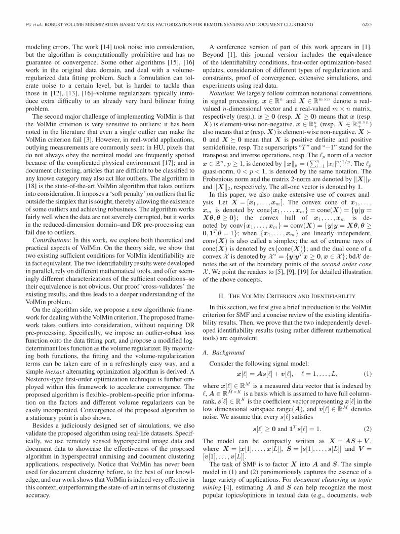
Fig. 1. Motivating examples: Hyperspectral unmixing and documentclustering.
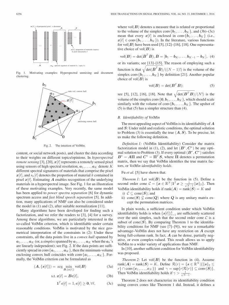
Fig. 2. The intuition of VolMin.
content, or social network posts), and cluster the data accordingto their weights on different topics/opinions. In hyperspectralremote sensing [3], [20], x[�] represents a remotely sensed pixelusing sensors of high spectral resolution, a1 , . . . ,aK denote Kdifferent spectral signatures of materials that comprise the pixelx[�], and sk [�] denotes the proportion of material k contained inpixel x[�]. Estimating A enables recognition of the underlyingmaterials in a hyperspectral image. See Fig. 1 for an illustrationof these motivating examples. Very recently, the same modelhas been applied to power spectra separation [6] for dynamicspectrum access and fast blind speech separation [5]. In addi-tion, many applications of NMF can also be considered underthe model in (1) and (2), after suitable normalization [11].
Many algorithms have been developed for finding such afactorization, and we refer the readers to [3], [4] for a survey.Among these algorithms, we are particularly interested in theso-called VolMin criterion, which is identifiable under certainreasonable conditions. VolMin is motivated by the nice geo-metrical interpretation of the constraints in (2): Under theseconstraints, all the data points live in a convex hull spanned bya1 , . . . ,aK (or, a simplex spanned by a1 , . . . ,aK when the ak ’sare linearly independent); see Fig. 2. If the data points are suffi-ciently spread in conv{a1 , . . . ,aK }, then the minimum-volumeenclosing convex hull coincides with conv{a1 , . . . ,aK }. For-mally, the VolMin criterion can be formulated as
(A, {s[�]}) = arg minB,{c[�]}
vol(B) (3a)
s.t. x[�] = Bc[�], (3b)
1T c[�] = 1, c[�] ≥ 0,∀�, (3c)
where vol(B) denotes a measure that is related or proportionalto the volume of the simplex conv{b1 , . . . , bK }, and (3b)–(3c)mean that every x[�] is enclosed in conv{b1 , . . . , bK } (i.e.,x[�] ∈ conv{b1 , . . . , bK }). In the literature, various functionsfor vol(B) have been used [5], [12]–[16], [18]. One representa-tive choice of vol(B) is
vol(B) = det(BTB), B = [b1 − bK , . . . , bK−1 − bK ], (4)
or its variants; see [13]–[15]. The reason of employing such a
function is that√
det(BTB)/((N − 1)!) is the volume of the
simplex conv{b1 , . . . , bK } by definition [21]. Another popularchoice of vol(B) is
vol(B) = det(BT B); (5)
see [5], [12], [16], [18]. Note that√
det(BT B)/(N !) is thevolume of the simplex conv{0, b1 , . . . , bK }, which should scalesimilarly with the volume of conv{b1 , . . . , bK }. The upshot of(5) is that (5) has a simpler structure than (4).
B. Identifiability of VolMin
The most appealing aspect of VolMin is its identifiability of Aand S: Under mild and realistic conditions, the optimal solutionto Problem (3) is essentially the true (A,S). To be precise, letus make the following definition.
Definition 1: (VolMin Identifiability) Consider the matrixfactorization model in (1), (2), and let (B� ,C�) be any opti-mal solution to Problem (3). If every optimal (B� ,C�) satisfiesB� = AΠ and C� = ΠT S, where Π denotes a permutationmatrix, then we say that VolMin identifies the true matrix fac-tors, or VolMin identifiability holds.
Fu et al. [5] have shown that.
Theorem 1: Let vol(B) be the function in (5). Define asecond order cone C = {x ∈ RN |1T x ≥ 1√
N −1‖x‖2}. Then
VolMin identifiability holds if rank(A) = rank(S) = K andi) C ⊆ cone(S); and
ii) cone(S) �⊆ cone(Q) where Q is any unitary matrix ex-cept the permutation matrices.
In plain words, a sufficient condition under which VolMinidentifiability holds is when {s[�]}L
�=1 are sufficiently scatteredover the unit simplex, such that the second order cone C is asubset of cone(S). By comparing Theorem 1 to the identifia-bility conditions for NMF (see [7]–[9]), we see a remarkableadvantage–VolMin does not have any restriction on A exceptbeing full-column rank. In fact, A can be dense, partially neg-ative, or even complex-valued. This result allows us to applyVolMin to a wider variety of applications than NMF.
In [10], another sufficient condition for VolMin identifiabilitywas proposed.
Theorem 2: Let vol(B) be the function in (4). Assumerank(A) = rank(S) = K. Define R(r) = {s ∈ RN |{‖s‖2 ≤r} ∩ conv{e1 , . . . ,eN }} and γ = sup{r|R(r)} ⊆ conv(S)}.Then VolMin identifiability holds if γ > 1√
N −1.
Theorem 2 does not characterize its identifiability conditionusing convex cones like Theorem 1 did. Instead, it defines a
FU et al.: ROBUST VOLUME MINIMIZATION-BASED MATRIX FACTORIZATION FOR REMOTE SENSING AND DOCUMENT CLUSTERING 6257
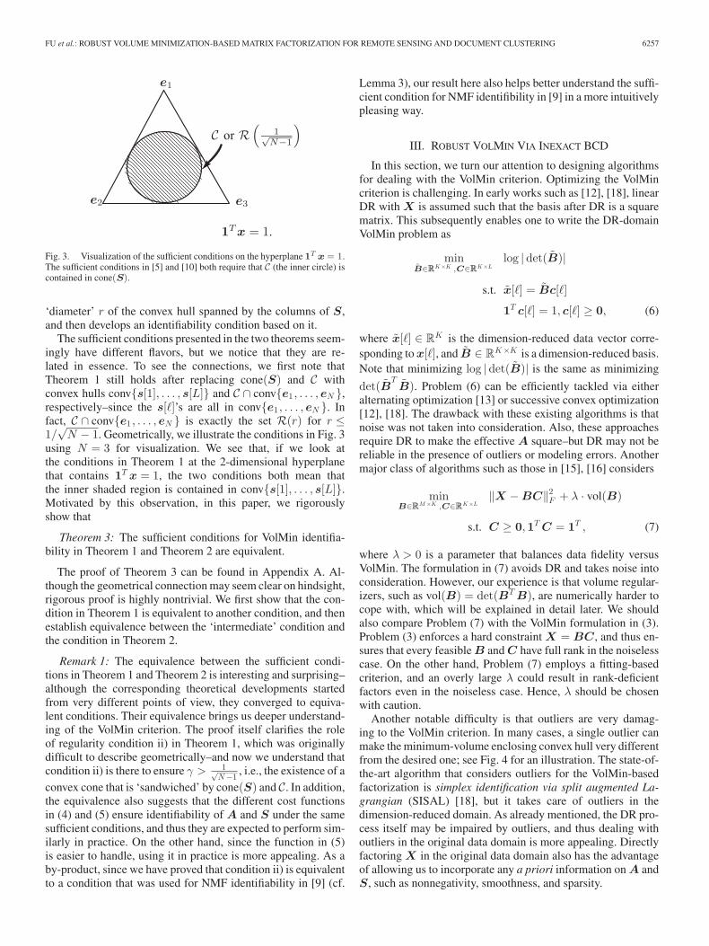
Fig. 3. Visualization of the sufficient conditions on the hyperplane 1T x = 1.The sufficient conditions in [5] and [10] both require that C (the inner circle) iscontained in cone(S).
‘diameter’ r of the convex hull spanned by the columns of S,and then develops an identifiability condition based on it.
The sufficient conditions presented in the two theorems seem-ingly have different flavors, but we notice that they are re-lated in essence. To see the connections, we first note thatTheorem 1 still holds after replacing cone(S) and C withconvex hulls conv{s[1], . . . , s[L]} and C ∩ conv{e1 , . . . ,eN },respectively–since the s[�]’s are all in conv{e1 , . . . ,eN }. Infact, C ∩ conv{e1 , . . . ,eN } is exactly the set R(r) for r ≤1/√
N − 1. Geometrically, we illustrate the conditions in Fig. 3using N = 3 for visualization. We see that, if we look atthe conditions in Theorem 1 at the 2-dimensional hyperplanethat contains 1T x = 1, the two conditions both mean thatthe inner shaded region is contained in conv{s[1], . . . , s[L]}.Motivated by this observation, in this paper, we rigorouslyshow that
Theorem 3: The sufficient conditions for VolMin identifia-bility in Theorem 1 and Theorem 2 are equivalent.
The proof of Theorem 3 can be found in Appendix A. Al-though the geometrical connection may seem clear on hindsight,rigorous proof is highly nontrivial. We first show that the con-dition in Theorem 1 is equivalent to another condition, and thenestablish equivalence between the ‘intermediate’ condition andthe condition in Theorem 2.
Remark 1: The equivalence between the sufficient condi-tions in Theorem 1 and Theorem 2 is interesting and surprising–although the corresponding theoretical developments startedfrom very different points of view, they converged to equiva-lent conditions. Their equivalence brings us deeper understand-ing of the VolMin criterion. The proof itself clarifies the roleof regularity condition ii) in Theorem 1, which was originallydifficult to describe geometrically–and now we understand thatcondition ii) is there to ensure γ > 1√
N −1, i.e., the existence of a
convex cone that is ‘sandwiched’ by cone(S) and C. In addition,the equivalence also suggests that the different cost functionsin (4) and (5) ensure identifiability of A and S under the samesufficient conditions, and thus they are expected to perform sim-ilarly in practice. On the other hand, since the function in (5)is easier to handle, using it in practice is more appealing. As aby-product, since we have proved that condition ii) is equivalentto a condition that was used for NMF identifiability in [9] (cf.
Lemma 3), our result here also helps better understand the suffi-cient condition for NMF identifibility in [9] in a more intuitivelypleasing way.
III. ROBUST VOLMIN VIA INEXACT BCD
In this section, we turn our attention to designing algorithmsfor dealing with the VolMin criterion. Optimizing the VolMincriterion is challenging. In early works such as [12], [18], linearDR with X is assumed such that the basis after DR is a squarematrix. This subsequently enables one to write the DR-domainVolMin problem as
minB∈RK×K ,C∈RK×L
log |det(B)|
s.t. x[�] = Bc[�]
1T c[�] = 1, c[�] ≥ 0, (6)
where x[�] ∈ RK is the dimension-reduced data vector corre-sponding to x[�], and B ∈ RK×K is a dimension-reduced basis.Note that minimizing log |det(B)| is the same as minimizing
det(BTB). Problem (6) can be efficiently tackled via either
alternating optimization [13] or successive convex optimization[12], [18]. The drawback with these existing algorithms is thatnoise was not taken into consideration. Also, these approachesrequire DR to make the effective A square–but DR may not bereliable in the presence of outliers or modeling errors. Anothermajor class of algorithms such as those in [15], [16] considers
minB∈RM ×K ,C∈RK×L
‖X − BC‖2F + λ · vol(B)
s.t. C ≥ 0,1T C = 1T , (7)
where λ > 0 is a parameter that balances data fidelity versusVolMin. The formulation in (7) avoids DR and takes noise intoconsideration. However, our experience is that volume regular-izers, such as vol(B) = det(BT B), are numerically harder tocope with, which will be explained in detail later. We shouldalso compare Problem (7) with the VolMin formulation in (3).Problem (3) enforces a hard constraint X = BC, and thus en-sures that every feasible B and C have full rank in the noiselesscase. On the other hand, Problem (7) employs a fitting-basedcriterion, and an overly large λ could result in rank-deficientfactors even in the noiseless case. Hence, λ should be chosenwith caution.
Another notable difficulty is that outliers are very damag-ing to the VolMin criterion. In many cases, a single outlier canmake the minimum-volume enclosing convex hull very differentfrom the desired one; see Fig. 4 for an illustration. The state-of-the-art algorithm that considers outliers for the VolMin-basedfactorization is simplex identification via split augmented La-grangian (SISAL) [18], but it takes care of outliers in thedimension-reduced domain. As already mentioned, the DR pro-cess itself may be impaired by outliers, and thus dealing withoutliers in the original data domain is more appealing. Directlyfactoring X in the original data domain also has the advantageof allowing us to incorporate any a priori information on A andS, such as nonnegativity, smoothness, and sparsity.

6258 IEEE TRANSACTIONS ON SIGNAL PROCESSING, VOL. 64, NO. 23, DECEMBER 1, 2016
Fig. 4. The impact of outliers to VolMin. The dots are x[�]’s; the shaded areais conv{a1 , . . . , aN }, the triangles with dashed lines are data-enclosing convexhulls, and the one with solid lines is the minimum-volume enclosing convexhull. Left: the case where no outliers exist. Right: the case where a single outlierexists.
A. Proposed Robust VolMin Algorithm
We are interested in the VolMin-regularized matrix factor-ization, but we take the outlier problem into consideration.Specifically, we propose to employ the following optimizationsurrogate of the VolMin criterion:
minB,C
L∑
�=1
12
(‖x[�] − Bc[�]‖2
2 + ε) p
2+
λ
2log det(BT B + τI)
s.t. 1T c[�] = 1, c[�] ≥ 0,∀�, (8)
where p ∈ (0, 2], λ > 0, ε > 0, and τ > 0. Here, ε > 0 is a smallregularization parameter, which keeps the first term inside itssmooth region for computational convenience when p < 1; ifp ∈ (1, 2], we can simply let ε = 0. The parameter τ > 0 is alsoa small positive number, which is used to ensure that the costfunction is bounded from below for any B.
The motivation of using log det(BT B + τI) instead of thecommonly used volume regularizers such as det(BT B) is com-putational simplicity: Although both functions are non-convexand conceptually equally hard to deal with, the former featuresa much simpler update rule because it admits a tight upperbound while the latter does not–this point will become clearershortly. Interestingly, log det(BT B + τI) has been used inthe context of low-rank matrix recovery [22], [23], but herewe instead apply it for simplex-VolMin. The �2/�p -(quasi-)norm data fitting part is employed to downweight the impactof the outliers–when 0 < p < 2, such a fitting criterion is lesssensitive to large fitting errors and thus is robust against out-liers. Other robust fitting criteria can also be considered–e.g.,the �p norm-based criterion ‖X − BC‖p
p for 0 < p < 2 where‖Y ‖p
p =∑m
i=1∑m
j=1 |Yi,j |p is known to be robust to entry-level outliers [24]–[26]. Nevertheless, the type of outliers thatmatters in VolMin is column outliers (or gross outliers) whichrepresents a point lying outside the ground-truth convex hull,and the proposed criterion is natural for fending against suchoutliers. In addition, computationally, the �2/�p mixed-normcriterion can be handled efficiently, as we will see.
Our primary objective is to handle Problem (8) efficiently.Nonetheless, we will also show that the proposed algorithmicframework can easily incorporate different volume-associatedregularizers in the literature, such as the previously mentionedvol(B) = det(BT B), and
vol(B) =K−1∑
i=1
K∑
j=i+1
‖bi − bj‖22 ; (9)
see [27]. Notice that (9) is a coarse approximation of the volumeof conv{b1 , . . . , bK }, which measures the volume by simplyadding up the squared distances between the vertices.
B. Update of C
Our idea is to update B and C alternately, i.e., using blockcoordinate descent (BCD). Unlike classic BCD [28], we solvethe partial optimization problems in an inexact fashion for effi-ciency. We first consider updating C. The problem w.r.t. C isseparable w.r.t. � and convex. Therefore, after t iterations withthe current solution (Bt ,Ct), we consider:
ct+1[�] := arg minc[�]
12
∥∥x[�] − Btc[�]
∥∥2
2
s.t. 1T c[�] = 1, c[�] ≥ 0, (10)
for � = 1, . . . , L. Since Problem (10) is convex, one can updateC by solving Problem (10) to optimality. An alternating direc-tion method of multipliers (ADMM)-based algorithm was pro-vided in the conference version of this work for this purpose; seethe detailed implementation in [1]. Nevertheless, exactly solv-ing Problem (10) at each iteration is computationally costly,especially when the problem size is large. Here, we propose todeal with Problem (10) using local approximation. Specifically,let
f(c[�];Bt) =12‖x[�] − Btc[�]‖2
2 .
Then, f(c[�];Bt) can be locally approximated at ct [�] by thefollowing:
u(c[�];Bt) = f(ct [�];Bt) +(∇f(ct [�];Bt)
)T (c[�] − ct [�])
+Lt
2‖c[�] − ct [�]‖2
2 ,
where Lt ≥ 0. On the right hand side (RHS) of the above,the first two terms constitute a first-order approximation off(c[�];Bt) at ct [�], and the second term restrains ct+1[�] to beclose to ct [�] in terms of Euclidean distance. It is well-knownthat when Lt ≥ ‖(Bt)T Bt‖2 ,
u(c[�];Bt) ≥ f(c[�];Bt),∀c[�] ∈ RK
holds for all c[�] and the equality holds if and only if c[�] =ct [�] [29]. In other words, when Lt ≥ ‖(Bt)T Bt‖2 , u(c[�]) isa ‘majorizing’ function of f(c[�];Bt). Given this majorizingfunction, we update c[�] by the following simple rule:
ct+1[�] = arg min1T c[�]=1,c[�]≥0
u(c[�];Bt). (11)
By re-arranging the terms and discarding constants, Prob-lem (11) is equivalent to the following
min1T c[�]=1,c[�]≥0
∥∥∥∥c[�] −
(
ct [�] − 1Lt
∇f(ct [�];Bt))∥
∥∥∥
2
2.
The RHS of the above can be considered as a gradient pro-jection step with step size 1/Lt . Letting PLt (ct [�]) denote theoptimal solution of the above, we simplify the notation of up-dating c[�] as
ct+1[�] = PLt (ct [�]). (12)
FU et al.: ROBUST VOLUME MINIMIZATION-BASED MATRIX FACTORIZATION FOR REMOTE SENSING AND DOCUMENT CLUSTERING 6259
Problem (12) is a simple projection that can be solved withworst-case complexity of O(K log K) flops; see [30] for a de-tailed implementation.
The described update of C has light per-iteration complexity,but it could result in slow convergence of the overall alternat-ing optimization algorithm; see Fig. 6 in the simulations. Toimprove the convergence speed in practice, and inspired by thesuccess of Nesterov’s optimal first-order algorithm and its re-lated algorithms [31], [32], we propose the following updateof C:
ct+1[�] = PLt (yt [�]) (13a)
qt+1 =1 +
√1 + 4(qt)2
2(13b)
yt [�] = ct [�] +(
qt − 1qt+1
)(ct [�] − ct−1 [�]
), (13c)
where {qt}∞t=1 is a sequence with q1 = 1. Simply speaking, in-stead of locally approximating f(c[�];Bt) at ct [�], we approx-imate it at an ‘extrapolated point’ yt [�]. Without the alternatingoptimization procedure, using extrapolation is provably muchfaster than using the plain gradient-based methods [31], [32].Embedding extrapolation into alternating optimization was firstconsidered in [33] in the context of tensor factorization, whereacceleration of convergence was observed. In our case, the ex-trapolation procedure also substantially reduces the number ofiterations for achieving convergence, as will be shown in thesimulations.
C. Update of B
The update of B relies on the following two lemmas.
Lemma 1: [34] Assume 0 < p ≤ 2, ε > 0, and letφp(w) := 2−p
2 ( 2p w)
pp −2 + εw. Then, we have (x2 + ε)p/2 =
minw≥0 wx2 + φp(w). Also, the minimizer is unique and givenby wopt = p
2 (x2 + ε)p −2
2 .
Lemma 2: [35] Let E ∈ RK×K be any matrix such thatE � 0. Consider the function f(F ) = Tr(FE) − log det F −K. Then, log det E = minF�0 f(F ), and the minimizer isuniquely given by F opt = E−1 .
The lemmas provide two functions that majorize the datafitting part and the volume-regularization part in (8), respec-tively. Specifically, at iteration t and after updating C, we have
(Bt, {ct+1[�]}L
�=1). Then, the following holds:
log det(BT B + εI) ≤ Tr(F tBT B) − log det F t − K,(14)
where F t = ((Bt)T Bt + εI)−1 and the equality holds whenB = Bt . Similarly, we have
L∑
�=1
12
(∥∥x[�] − Bct+1[�]
∥∥2
2 + ε) p
2
≤L∑
�=1
wt�
2
∥∥x[�] − Bct+1[�]
∥∥2
2 +L∑
�=1
φp(wt�), (15)
where wt� = p
2 (‖x − Btct+1[�]‖22 + ε)
p −22 and the equality
holds when B = Bt . Putting (14), (15) together and dropping
the irrelevant terms, we find Bt+1 by solving the following:
Bt+1 := arg minB
L∑
�=1
w�
2
∥∥x[�] − Bct+1[�]
∥∥2
2
+λ
2Tr(F t(BT B)). (16)
Problem (16) is a convex quadratic program that admits thefollowing closed-form solution:
Bt+1 := XW t(Ct+1)T(Ct+1W (Ct+1)T + λF t
)−1,
(17)
where W t = Diag(wt1 , . . . , w
tL ).
Remark 2: The expression in (16) reveals why the proposedcriterion and algorithm can automatically downweight the effectbrought by the outliers. Suppose that (Bt ,Ct+1) is a “goodenough” solution which is close to the ground truth. Then, wt
� issmall when x[�] is an outlier since the fitting error term ‖x[�] −Btct+1[�]‖2
2 is large. Hence, for the next iteration, Bt+1 isestimated with the importance of the outlier x[�] downweighted.
Remark 3: In practice, adding constraints on B by lettingB ∈ B is sometimes instrumental, since a lot of applications dohave prior information that can be used to enhance performance.For example, in image processing, a nonnegative B is oftensought, and thus one can set B = RM ×N
+ . When B is convex,the problem in (16) can usually be solved in an efficient man-ner; e.g., one can call general-purpose solvers such as interior-point methods. However, using general-purpose solvers heremay lose efficiency since solving constrained least squares to acertain accuracy per se may require a lot of iterations. To sim-plify the update, we update Bt following the same spirit of up-dating C: Let g(B;Ct+1) =
∑L�=1
w�
2 ‖x[�] − Bct+1[�]‖22 +
λ2 Tr(F t(BT B)) + const, where const =
∑L�=1 φp(wt
�) − K.We solve a local approximation of g(B;Ct+1):
Bt+1 := arg minB∈B
g(Bt ;Ct+1) + ∇g(Bt ;Ct+1)T (B − Bt)
+μt
2‖B − Bt‖2
F
:= ProjB(Bt − μt∇g(Bt ;Ct+1)
), (18)
where μt ≥ 0 and
∇g(Bt ;Ct+1) = Bt(Ct+1W t(Ct+1)T + λF t
)
− XW t(Ct+1)T ,
is the partial derivative of the cost function in (16) w.r.t. B atBt , and ProjB(Z) denotes the Euclidean projection of Z onB. For some B’s, the projection is easy to compute; e.g., whenB = RM
+ , we have ProjB(Z) = max{Z,0}; see other easilyimplementable projections in [36]. Notice that the update in(18) can also easily incorporate extrapolation.
The robust volume minimization (RVolMin) algorithm issummarized in Algorithm 1. Its convergence properties arestated in Proposition 1, whose proof is relegated to Appendix B.
Proposition 1: Assume that Lt and μt are chosen such thatLt ≥ ‖(Bt)T Bt‖2 and μt ≥ ‖(F t)T F t‖2 , respectively. Also,

6260 IEEE TRANSACTIONS ON SIGNAL PROCESSING, VOL. 64, NO. 23, DECEMBER 1, 2016
assume that B is a convex closed set. Then, if the initial objec-tive value is finite, the whole solution sequence generated byAlgorithm 1 converges to the set S that consists of all the sta-tionary points of Problem (8), i.e.,
limt→∞
d(t) ((Bt ,Ct
),S
)= 0,
where d(t)((Bt ,Ct),S) = minY ∈S ‖Y − (Bt ,Ct)‖2F .
Remark 4: As mentioned before, we may also use differentvolume regularizers. Let us consider the volume regularizer in(9) first. It was shown in [27] that this regularizer can also beexpressed as vol(B) = Tr(GBT B), where G = KI − 11T .Therefore, by letting F t = G in Algorithm 1, the updates canbe directly applied to handle the regularizer in (9). Dealing with(5) is more difficult. One possible way is to make use of (18)since det(BT B) is differentiable. The difficulty is that a globalupper bound of the subproblem w.r.t. B may not exist. Undersuch circumstances, sufficient decrease at each iteration needsto be guaranteed for establishing convergence to a stationarypoint [37]. In practice, the Armijo rule is usually invoked toachieve this goal, which in general is computationally morecostly compared to the cases where μt can be determined inclosed form.
Remark 5: Problem (8) is a nonconvex optimization prob-lem. Hence, a good starting point of RVolMin can help reachmeaningful solutions quickly. In practice, different initializa-tions can be considered:• Existing VolMin algorithms. Many VolMin algorithms, suchas the ones working in the reduced-dimension domain (e.g., thealgorithms in [13], [18]), exhibit good efficiency. The difficultyis that these algorithms are usually sensitive to the DR processin the presence of outliers. Nevertheless, one can employ robustDR algorithms together with the algorithms in [13], [18] as aninitialization approach. Nuclear norm-based algorithms [38] areviable options for robust DR, but are not suitable for large-scaleproblems because of the computational complexity. Under suchcircumstances, one may adopt simple alternatives such as thatproposed in [39].• Nonnegative matrix factorization. If A is known to be non-negative, any NMF algorithm can be employed as initialization.In practice, dealing with NMF is arguably simpler relative toVolMin, and many efficient solvers for NMF exist–see [40] fora survey. Although NMF usually does not provide a satisfac-tory result on its own in cases where it cannot guarantee theidentifiability of its factors, using the NMF-estimated factors to
initialize the algorithms that provide identifiability guaranteescan sometimes enhance the performance of the latter.
IV. SIMULATIONS
In this section, we provide simulations to showcase the ef-fectiveness of the proposed algorithm. We generate the ele-ments of A ∈ RM ×K from the uniform distribution betweenzero and one. We generate s[�] on the unit simplex andwith maxi si [�] ≤ γ, where 1
K ≤ γ ≤ 1 is given. We chooseγ = 0.85, which results in a so-called ‘no-pure-pixel case’ inthe context of remote sensing and is known to be challengingto handle; see [3], [4] for details. Zero-mean white Gaussiannoise is added to the generated data. To model outliers, we de-fine the outlier at data point � as o[�] and let A ⊆ {1, . . . , L} bethe index set of outliers. We assume that o[�] = 0 if � /∈ A andx[�] = o[�] otherwise. We denote No = |A| as the total num-ber of outliers. Those active outliers are generated following theuniform distribution between zero and one, and are scaled to sat-isfy problem specifications. For the proposed algorithm, we fixp = 0.5, ε = 10−12 , and τ = 10−8 unless otherwise specified.We stop the proposed algorithm when the absolute change ofthe cost function is smaller than 10−5 or the number of iterationsreaches 1000.
We define the signal-to-noise ratio (SNR) as SNR =10 log10(
E{‖As[�]‖22 }
E{‖v[�]‖22 }
). Also, to quantify the corruption causedby the outliers, we define the signal-to-outlier ratio (SOR) as
SOR = 10 log10(E{‖As[�]‖2
2 }E{‖o[�]‖2
2 }). We use the mean-squared-error
(MSE) of A as a measure of factorization performance, definedas
MSE = minπ∈Π
1K
K∑
k=1
∥∥∥∥
ak
‖ak‖2− aπk
‖aπk‖2
∥∥∥∥
2
2,
where Π is the set of all permutations of {1, 2, . . . ,K}; and ak
is the estimate of ak .In this section, we use the SISAL algorithm proposed in [18]
as a baseline. SISAL is a state-of-art robust VolMin algorithmthat takes outliers into account by solving
minB,1T C=1T ,{x[�]=Bc[�]}
log det(B) + η‖C‖h ,
where ‖ · ‖h =∑L
�=1∑K
k=1 max(−ck [�], 0) is an element-wisehinge function. The intuition behind SISAL is to penalize theoutliers whose c[�] has negative elements, but still allowingthem to exist, thereby having some robustness to outliers. Thetuning parameter η > 0 in SISAL controls the amount of outliersthat are “allowed,” and we test multiple η’s for SISAL in thesimulations. We run the original SISAL that uses SVD-baseddimension reduction and the modified SISAL which uses therobust dimension reduction (RDR) algorithm in [39]. The latteris also used to initialize the proposed algorithm.
We first use an illustrative example to show the effective-ness of the proposed algorithm in the presence of outliers. Inthis example, we set SNR = 18 dB, SOR = −10 dB, No =20, (M,K) = (50, 3), and L = 1000. The results are pro-jected onto the affine set that contains conv{a1 ,a2 ,a3}, i.e., atwo-dimensional hyperplane. In Fig. 5, we see that SISAL withdifferent η’s cannot yield reasonable estimates of A since the
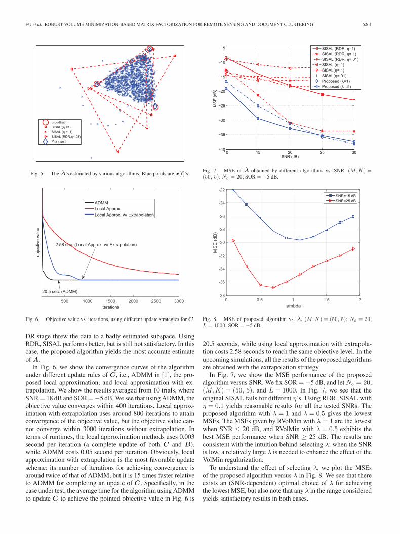
FU et al.: ROBUST VOLUME MINIMIZATION-BASED MATRIX FACTORIZATION FOR REMOTE SENSING AND DOCUMENT CLUSTERING 6261
Fig. 5. The A’s estimated by various algorithms. Blue points are x[�]’s.
Fig. 6. Objective value vs. iterations, using different update strategies for C.
DR stage threw the data to a badly estimated subspace. UsingRDR, SISAL performs better, but is still not satisfactory. In thiscase, the proposed algorithm yields the most accurate estimateof A.
In Fig. 6, we show the convergence curves of the algorithmunder different update rules of C, i.e., ADMM in [1], the pro-posed local approximation, and local approximation with ex-trapolation. We show the results averaged from 10 trials, whereSNR = 18 dB and SOR =−5 dB. We see that using ADMM, theobjective value converges within 400 iterations. Local approx-imation with extrapolation uses around 800 iterations to attainconvergence of the objective value, but the objective value can-not converge within 3000 iterations without extrapolation. Interms of runtimes, the local approximation methods uses 0.003second per iteration (a complete update of both C and B),while ADMM costs 0.05 second per iteration. Obviously, localapproximation with extrapolation is the most favorable updatescheme: its number of iterations for achieving convergence isaround twice of that of ADMM, but it is 15 times faster relativeto ADMM for completing an update of C. Specifically, in thecase under test, the average time for the algorithm using ADMMto update C to achieve the pointed objective value in Fig. 6 is
Fig. 7. MSE of A obtained by different algorithms vs. SNR. (M, K ) =(50, 5); No = 20; SOR = −5 dB.
Fig. 8. MSE of proposed algorithm vs. λ. (M, K ) = (50, 5); No = 20;L = 1000; SOR = −5 dB.
20.5 seconds, while using local approximation with extrapola-tion costs 2.58 seconds to reach the same objective level. In theupcoming simulations, all the results of the proposed algorithmsare obtained with the extrapolation strategy.
In Fig. 7, we show the MSE performance of the proposedalgorithm versus SNR. We fix SOR = −5 dB, and let No = 20,(M,K) = (50, 5), and L = 1000. In Fig. 7, we see that theoriginal SISAL fails for different η’s. Using RDR, SISAL withη = 0.1 yields reasonable results for all the tested SNRs. Theproposed algorithm with λ = 1 and λ = 0.5 gives the lowestMSEs. The MSEs given by RVolMin with λ = 1 are the lowestwhen SNR ≤ 20 dB, and RVolMin with λ = 0.5 exhibits thebest MSE performance when SNR ≥ 25 dB. The results areconsistent with the intuition behind selecting λ: when the SNRis low, a relatively large λ is needed to enhance the effect of theVolMin regularization.
To understand the effect of selecting λ, we plot the MSEsof the proposed algorithm versus λ in Fig. 8. We see that thereexists an (SNR-dependent) optimal choice of λ for achievingthe lowest MSE, but also note that any λ in the range consideredyields satisfactory results in both cases.

6262 IEEE TRANSACTIONS ON SIGNAL PROCESSING, VOL. 64, NO. 23, DECEMBER 1, 2016
Fig. 9. MSE of A versus K . M = 50; No = 20; L = 1000; SOR = −5 dB.
Fig. 10. MSE of A versus SOR. (M, K ) = (50, 5); No = 20; L = 1000;SNR = 20 dB.
Fig. 9 shows the MSE performance of the algorithms versusK. We fix SNR = 20 dB and the other settings are the sameas in the previous simulation. The results of SISAL and SISALwith RDR are also used as baselines. We run several η’s forSISAL and present the results of the one with the lowest MSEs.As expected, all the algorithms work better when the rank ofthe factorization model is lower–which is consistent with pastexperience on different matrix factorization algorithms, suchas [40]. SISAL and SISAL with RDR work reasonably whenK = 3, but deteriorate when K ≥ 6. On the other hand, evenwhen K = 15, the proposed algorithm still works well, givingthe lowest MSE.
Fig. 10 shows the MSEs of the algorithms versus SORs. Onecan see that when some data are badly corrupted, i.e., whenSOR ≤ −10 dB, the proposed algorithm yields significantlylower MSEs than SISAL and SISAL with RDR. When SOR ≥0 dB, all three algorithms provide comparable performance.
We also test the algorithms versus the number of outliers.In Fig. 11, one can see that the proposed algorithm is not verysensitive to the change of No : the MSE curve of the proposed al-gorithm is quite flat for different No ’s in this simulation. SISAL
Fig. 11. MSE of A versus No . (M, K ) = (50, 5); L = 1000; SOR =−5 dB; SNR = 20 dB.
TABLE ITHE MSES OF THE ALGORITHMS UNDER ILL-CONDITIONED A.
(M, K ) = (50, 5); L = 1000; No = 20; SOR = −5 DB.
TABLE IITHE MSES OF THE PROPOSED ALGORITHM WITH DIFFERENT VOL(B)’S.
(M, K ) = (50, 5); L = 1000; No = 20; SNR = 20 DB.
with RDR yields reasonable MSEs when No ≤ 40, but its per-formance deteriorates when No is larger.
Table I presents the MSEs of the estimated A under well- andill-conditioned A’s, respectively. To generate an ill-conditionedA, we use a way that is similar to the method suggestedin [11]: in each trial, we first generate A whose columnsare uniformly distributed between zero and one, and suchA’s are relatively well-conditioned. Then, we apply singularvalue decomposition to obtain A = UΣV T . Finally, we re-place Σ by Σ = Diag([1, 0.1, 0.01, 0.005, 0.001]) and obtainA = UΣV T . This way, the condition number of the generatedA is 103 . The other settings are the same as those in Fig. 7.One can see from Table I that using such ill-conditioned A, allthe algorithms perform worse compared to the scenario whereA has uniformly distributed columns (cf. the first and secondcolumns in Table I). Nevertheless, the proposed algorithm stillgives the lowest MSEs.
In Table II, we present the MSE performance of the proposedalgorithm using different volume regularizers. We see that us-ing vol(B) = Tr(GBBT ) has the shortest runtime since the
FU et al.: ROBUST VOLUME MINIMIZATION-BASED MATRIX FACTORIZATION FOR REMOTE SENSING AND DOCUMENT CLUSTERING 6263
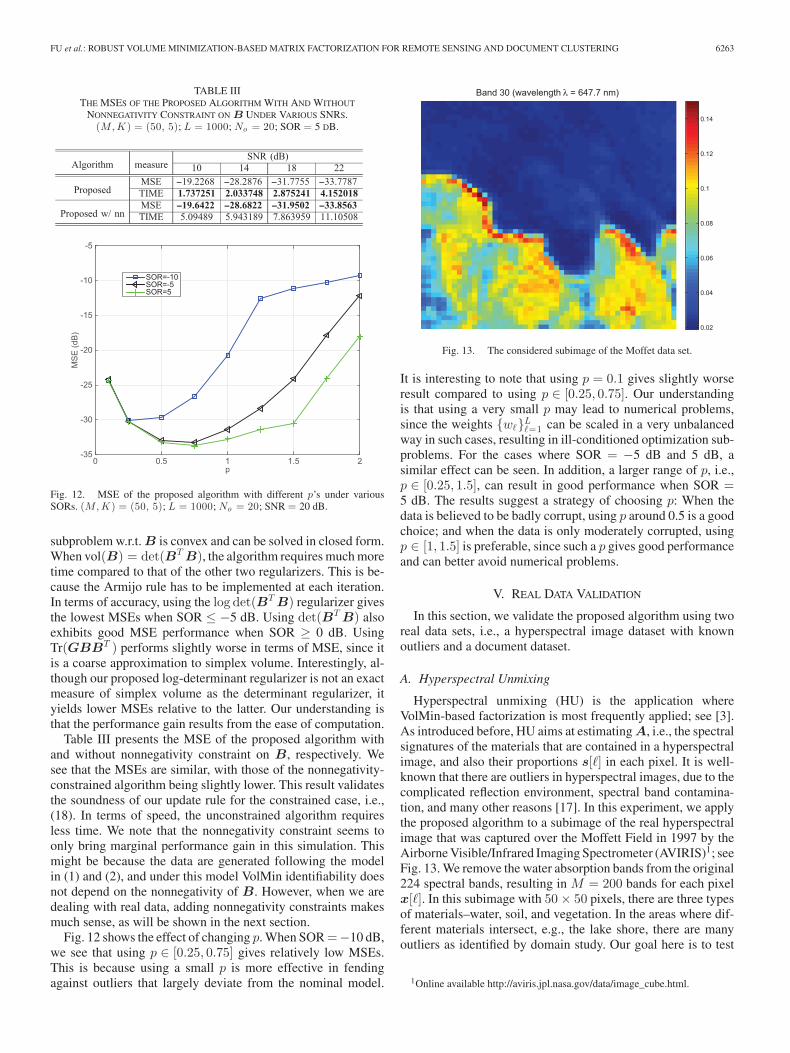
TABLE IIITHE MSES OF THE PROPOSED ALGORITHM WITH AND WITHOUT
NONNEGATIVITY CONSTRAINT ON B UNDER VARIOUS SNRS.(M, K ) = (50, 5); L = 1000; No = 20; SOR = 5 DB.
Fig. 12. MSE of the proposed algorithm with different p’s under variousSORs. (M, K ) = (50, 5); L = 1000; No = 20; SNR = 20 dB.
subproblem w.r.t. B is convex and can be solved in closed form.When vol(B) = det(BT B), the algorithm requires much moretime compared to that of the other two regularizers. This is be-cause the Armijo rule has to be implemented at each iteration.In terms of accuracy, using the log det(BT B) regularizer givesthe lowest MSEs when SOR ≤ −5 dB. Using det(BT B) alsoexhibits good MSE performance when SOR ≥ 0 dB. UsingTr(GBBT ) performs slightly worse in terms of MSE, since itis a coarse approximation to simplex volume. Interestingly, al-though our proposed log-determinant regularizer is not an exactmeasure of simplex volume as the determinant regularizer, ityields lower MSEs relative to the latter. Our understanding isthat the performance gain results from the ease of computation.
Table III presents the MSE of the proposed algorithm withand without nonnegativity constraint on B, respectively. Wesee that the MSEs are similar, with those of the nonnegativity-constrained algorithm being slightly lower. This result validatesthe soundness of our update rule for the constrained case, i.e.,(18). In terms of speed, the unconstrained algorithm requiresless time. We note that the nonnegativity constraint seems toonly bring marginal performance gain in this simulation. Thismight be because the data are generated following the modelin (1) and (2), and under this model VolMin identifiability doesnot depend on the nonnegativity of B. However, when we aredealing with real data, adding nonnegativity constraints makesmuch sense, as will be shown in the next section.
Fig. 12 shows the effect of changing p. When SOR =−10 dB,we see that using p ∈ [0.25, 0.75] gives relatively low MSEs.This is because using a small p is more effective in fendingagainst outliers that largely deviate from the nominal model.
Fig. 13. The considered subimage of the Moffet data set.
It is interesting to note that using p = 0.1 gives slightly worseresult compared to using p ∈ [0.25, 0.75]. Our understandingis that using a very small p may lead to numerical problems,since the weights {w�}L
�=1 can be scaled in a very unbalancedway in such cases, resulting in ill-conditioned optimization sub-problems. For the cases where SOR = −5 dB and 5 dB, asimilar effect can be seen. In addition, a larger range of p, i.e.,p ∈ [0.25, 1.5], can result in good performance when SOR =5 dB. The results suggest a strategy of choosing p: When thedata is believed to be badly corrupt, using p around 0.5 is a goodchoice; and when the data is only moderately corrupted, usingp ∈ [1, 1.5] is preferable, since such a p gives good performanceand can better avoid numerical problems.
V. REAL DATA VALIDATION
In this section, we validate the proposed algorithm using tworeal data sets, i.e., a hyperspectral image dataset with knownoutliers and a document dataset.
A. Hyperspectral Unmixing
Hyperspectral unmixing (HU) is the application whereVolMin-based factorization is most frequently applied; see [3].As introduced before, HU aims at estimating A, i.e., the spectralsignatures of the materials that are contained in a hyperspectralimage, and also their proportions s[�] in each pixel. It is well-known that there are outliers in hyperspectral images, due to thecomplicated reflection environment, spectral band contamina-tion, and many other reasons [17]. In this experiment, we applythe proposed algorithm to a subimage of the real hyperspectralimage that was captured over the Moffett Field in 1997 by theAirborne Visible/Infrared Imaging Spectrometer (AVIRIS)1; seeFig. 13. We remove the water absorption bands from the original224 spectral bands, resulting in M = 200 bands for each pixelx[�]. In this subimage with 50 × 50 pixels, there are three typesof materials–water, soil, and vegetation. In the areas where dif-ferent materials intersect, e.g., the lake shore, there are manyoutliers as identified by domain study. Our goal here is to test
1Online available http://aviris.jpl.nasa.gov/data/image_cube.html.
6264 IEEE TRANSACTIONS ON SIGNAL PROCESSING, VOL. 64, NO. 23, DECEMBER 1, 2016
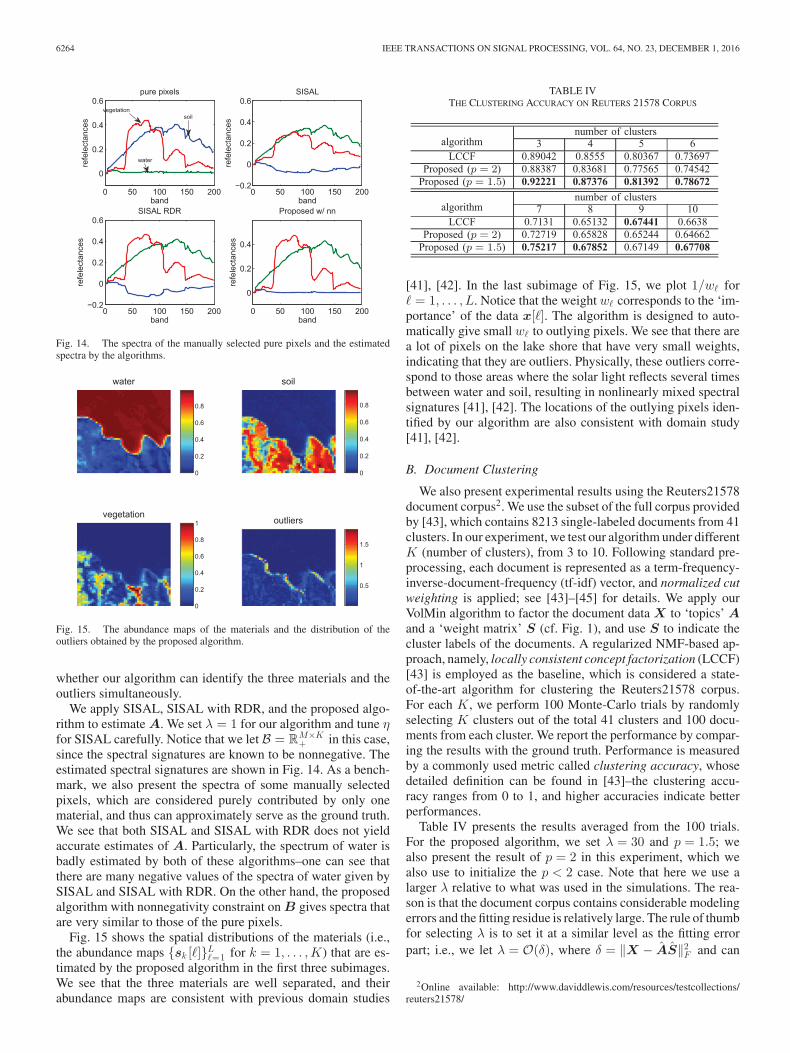
Fig. 14. The spectra of the manually selected pure pixels and the estimatedspectra by the algorithms.
Fig. 15. The abundance maps of the materials and the distribution of theoutliers obtained by the proposed algorithm.
whether our algorithm can identify the three materials and theoutliers simultaneously.
We apply SISAL, SISAL with RDR, and the proposed algo-rithm to estimate A. We set λ = 1 for our algorithm and tune ηfor SISAL carefully. Notice that we let B = RM×K
+ in this case,since the spectral signatures are known to be nonnegative. Theestimated spectral signatures are shown in Fig. 14. As a bench-mark, we also present the spectra of some manually selectedpixels, which are considered purely contributed by only onematerial, and thus can approximately serve as the ground truth.We see that both SISAL and SISAL with RDR does not yieldaccurate estimates of A. Particularly, the spectrum of water isbadly estimated by both of these algorithms–one can see thatthere are many negative values of the spectra of water given bySISAL and SISAL with RDR. On the other hand, the proposedalgorithm with nonnegativity constraint on B gives spectra thatare very similar to those of the pure pixels.
Fig. 15 shows the spatial distributions of the materials (i.e.,the abundance maps {sk [�]}L
�=1 for k = 1, . . . ,K) that are es-timated by the proposed algorithm in the first three subimages.We see that the three materials are well separated, and theirabundance maps are consistent with previous domain studies
TABLE IVTHE CLUSTERING ACCURACY ON REUTERS 21578 CORPUS
[41], [42]. In the last subimage of Fig. 15, we plot 1/w� for� = 1, . . . , L. Notice that the weight w� corresponds to the ‘im-portance’ of the data x[�]. The algorithm is designed to auto-matically give small w� to outlying pixels. We see that there area lot of pixels on the lake shore that have very small weights,indicating that they are outliers. Physically, these outliers corre-spond to those areas where the solar light reflects several timesbetween water and soil, resulting in nonlinearly mixed spectralsignatures [41], [42]. The locations of the outlying pixels iden-tified by our algorithm are also consistent with domain study[41], [42].
B. Document Clustering
We also present experimental results using the Reuters21578document corpus2. We use the subset of the full corpus providedby [43], which contains 8213 single-labeled documents from 41clusters. In our experiment, we test our algorithm under differentK (number of clusters), from 3 to 10. Following standard pre-processing, each document is represented as a term-frequency-inverse-document-frequency (tf-idf) vector, and normalized cutweighting is applied; see [43]–[45] for details. We apply ourVolMin algorithm to factor the document data X to ‘topics’ Aand a ‘weight matrix’ S (cf. Fig. 1), and use S to indicate thecluster labels of the documents. A regularized NMF-based ap-proach, namely, locally consistent concept factorization (LCCF)[43] is employed as the baseline, which is considered a state-of-the-art algorithm for clustering the Reuters21578 corpus.For each K, we perform 100 Monte-Carlo trials by randomlyselecting K clusters out of the total 41 clusters and 100 docu-ments from each cluster. We report the performance by compar-ing the results with the ground truth. Performance is measuredby a commonly used metric called clustering accuracy, whosedetailed definition can be found in [43]–the clustering accu-racy ranges from 0 to 1, and higher accuracies indicate betterperformances.
Table IV presents the results averaged from the 100 trials.For the proposed algorithm, we set λ = 30 and p = 1.5; wealso present the result of p = 2 in this experiment, which wealso use to initialize the p < 2 case. Note that here we use alarger λ relative to what was used in the simulations. The rea-son is that the document corpus contains considerable modelingerrors and the fitting residue is relatively large. The rule of thumbfor selecting λ is to set it at a similar level as the fitting errorpart; i.e., we let λ = O(δ), where δ = ‖X − AS‖2
F and can
2Online available: http://www.daviddlewis.com/resources/testcollections/reuters21578/
FU et al.: ROBUST VOLUME MINIMIZATION-BASED MATRIX FACTORIZATION FOR REMOTE SENSING AND DOCUMENT CLUSTERING 6265
be coarsely estimated using plain NMF. This way, λ can bal-ance the fitting part and the volume regularizer. From Table IV,we see that VolMin with p = 2 already yields comparable clus-tering accuracy with LCCF. This indicates that, even withoutoutlier-robustness, modeling the document clustering problemusing VolMin-based SMF is effective. Better accuracies can beseen by using p = 1.5, where we see that for most K, the pro-posed RVolMin algorithm gives the best accuracy. In particular,for K = 6, 7, more than 4% accuracy improvement can be seen,which is considered significant in the context of document clus-tering. Interestingly, further decreasing p does not yield betterperformance. This implies that the modeling error is not verysevere, but outliers do exist, since using p < 2 gives better clus-tering result than using p = 2 which is not robust to modelingerrors.
VI. CONCLUSION
In this work, we looked into theoretical and practical aspectsof the VolMin criterion for matrix factorization. On the theoryside, we showed that two independently developed sufficientconditions for VolMin identifiability are in fact equivalent. Onthe practical side, we proposed an outlier-robust optimizationsurrogate of the VolMin criterion, and devised an inexact BCDalgorithm to deal with it. Extensive simulations showed thatthe proposed algorithm outperforms a state-of-the-art robustVolMin algorithm, i.e., SISAL. The proposed algorithm wasalso validated using real-world hyperspectral image data anddocument data, where interesting and favorable results wereobserved.
APPENDIX A
A. Proof of Theorem 3
To show Theorem 3, several properties of convex cones willbe constantly used. They are:
Property 1: Let K1 and K2 be convex cones. Then, K1 ⊆K2 ⇒ K∗
2 ⊆ K∗1 .
Property 2: Let K1 and K2 be convex cones. Then, (K1 ∩K2)∗ = conv{K∗
1 ∪ K∗2}.
Property 3: If Q is a unitary matrix. Then, cone(Q)∗ =cone(Q).
We show Theorem 3 step by step. First, we show the followinglemma:
Lemma 3: Assume that C ⊆ cone(S) and Q is any uni-tary matrix except the permutation matrices. Then, wehave cone(S)∗ ∩ bdC∗ = {λiei |i = 1, . . . , N} ⇔ cone(S) �⊆cone(Q).
Proof: We first show the “⇒” part. Given a unitary Q, sup-pose that
cone(S) ⊆ cone(Q).
By the basic properties of convex cones, we see thatcone(Q)∗ ⊆ cone(S)∗, and cone(Q)∗ = cone(Q). Combining,we see
cone(Q) ⊆ cone(S)∗. (19)
Also, we have
C ⊆ cone(S) ⇒ cone(S)∗ ⊆ C∗ ⇒ cone(Q) ⊆ C∗. (20)
Combining Eqs. (19) and (20), we have
cone(Q) ⊆ C∗ ∩ cone(S)∗. (21)
We also know that the extreme rays of cone(Q) lie in theboundary of C∗, i.e., ex{cone(Q)} ⊆ bdC∗ [9, Lemma 1]. Thus,we have
ex{cone(Q)} ⊆ bdC∗ ∩ cone(S)∗. (22)
Since we assumed cone(S)∗ ∩ bdC∗ = {λiei |i = 1, . . . , N},we have
ex{cone(Q)} ⊆ {e1 , . . . ,eN }. (23)
Therefore, Q can only be a permutation matrix.We now show the “⇐” part. Following (22), and knowing
that cone(S) is a subset of the convex cone of some permutationmatrix, we see that
{e1 , . . . ,eN } ⊆ cone(S)∗ ∩ bdC∗. (24)
Now, suppose that there are a set of vectors {r1 , . . . , rp} thatdoes not include any unit vectors such that
cone(S)∗ ∩ bdC∗ = {e1 , . . . ,eN , r1 , . . . , rp}.
Then, we see that we can represent cone(S)∗ = conv{RN+ ∪
cone{r1 , . . . , rp}}. By Property 2, we see that
cone(S) = conv{RN+ ∪ cone{r1 , . . . , rp}}∗
= RN+ ∩ cone{r1 , . . . , rp}∗. (25)
Since RN+ ∩ cone{r1 , . . . , rp}∗ = cone(S) ⊆ RN
+ , (25)leads to
cone{r1 , . . . , rp}∗ ⊆ RN+ .
By Property 1, we see that
(RN+ )∗ = RN
+ ⊆ cone{r1 , . . . , rp}.
This is a contradiction to the assumption that {r1 , . . . , rp}does not include the unit vectors. �
Now we are ready to prove Theorem 3. We first noticethat C ⊆ cone(S) is equivalent to γ ≥ 1
N −1 . In fact, we seethat C ∩ S = R( 1√
N −1), where S = {s|1T s = 1, s ∈ RN },
and thus the claim holds. Thus, our remaining work is to showthat condition (ii) in Theorem 1 is equivalent to restricting γsuch that γ > 1√
N −1Step 1: Let us consider a conic representation of Theorem 2.
Specifically, the corresponding convex cone of R(r) = {s ∈RN |‖{s‖2 ≤ r} ∩ conv{e1 , . . . ,eN }} is R(r) = C(r) ∩RN
+ ,where
C(r) = {s ∈ RN | ‖s‖2 ≤ r1T s},
and γ = sup{r|C(r) ⊆ cone(S)} under this definition. It is alsonoticed that C(r) can be re-expressed as
C(r) ={
s∣∣∣∣
1T s‖1‖2‖s‖2
≥ 1r√
N
}
.
In words, the vectors whose angles between 1 are less thanor equal to arccos 1
r√
Ncomprises C(r). Therefore, by the def-
inition of dual cone, i.e., C(r)∗ = {s|sT y ≥ 0,y ∈ C}, C(r)∗
6266 IEEE TRANSACTIONS ON SIGNAL PROCESSING, VOL. 64, NO. 23, DECEMBER 1, 2016
contains all the vectors that have the angle with 1 less than orequal to arccos r√
r 2 N −1, which leads to
C(r)∗ = C(
r√r2N − 1
)
. (26)
Step 2: Now, we consider the dual cone representation ofTheorem 2. Let us define
T (r) = conv(C(r) ∪RN+ ).
Then, following Property 2 and (26), we have
R(r)∗ = (C(r) ∩RN+ )∗ (27a)
= conv
(
C(
r√r2N − 1
)
∪RN+
)
, (27b)
= T(
r√r2N − 1
)
, (27c)
where we have used (RN+ )∗ = RN
+ , i.e., Property 3. Accordingto Property 1, we see that
R(r) ⊆ cone(S) ⇔ cone(S)∗ ⊆ T(
r√r2N − 1
)
. (28)
If we define κ = inf{r|cone(S)∗ ⊆ T (r)}, we see from (28)and the definition of γ that
γ >1√
N − 1⇔ κ < 1. (29)
Step 3: To show the equivalence between the sufficient condi-tions, let us begin from Theorem 1. The condition C ⊆ cone(S)means that C∗ ⊆ cone(S)∗ by Property (1), and it further im-plies that {e1 , . . . ,eN } ⊆ ex{cone(S)∗} [9]. Suppose the restof cone(S)∗’s extreme rays are r1 , . . . , rp , and t is defined ast = inf{r|cone{r1 , . . . , rp} ⊆ C(r)}. Then, we have
cone(S)∗ = cone{r1 , . . . , rp ,e1 , . . . ,eN }
⊆ conv{C(t) ∪RN+ } = T (t).
Hence, by the definitions of t and κ, we have t = κ.Given the above analysis, we first show that Theorem 1 im-
plies Theorem 2. Now, assume that Condition (ii) in Theo-rem 1 is satisfied. We see that cone(S)∗ ∩ bdC∗ = {λiei |i =1, . . . , N} by Lemma 3. Then, r1 , . . . , rp are in the interior ofC∗ = C(1). Therefore, we have t < 1, and subsequently κ < 1and γ > 1√
N −1strictly.
Now we show the converse by contradiction. Assume thatγ > 1√
N −1holds (the condition in Theorem 2 is satisfied). If at
least one point in r1 , . . . , rp touches the boundary of C∗ (con-dition (ii) in Theorem 1 is not satisfied), then t = 1, and wecannot decrease it further while still contain cone(S)∗ in T (t)∗.This means that κ = 1, or, equivalently, γ = 1√
N −1, which con-
tradicts our first assumption that γ > 1√N −1
.
B. Proof of Proposition 1
In the following, we prove the proposition under the algo-rithmic structure without extrapolation. For the case where weupdate C using (13), it is easy to see that yt [�] → ct [�] given
t → ∞ by (13c). Hence, if the proposition holds for the algo-rithm without extrapolation, it also holds for the extrapolatedversion asymptotically.
First, let us cast the proposed algorithm into the frameworkof block successive upper bound minimization (BSUM) [29],[37]. Unlike the classic block coordinate descent algorithm thatsolves every block subproblem exactly [28], BSUM cyclicallysolves the upper-bound problems of every block subproblems.We consider the updates using (12) and (16) as an example. Theproof of using other updates will follow. Our update rule in (12)and (16) can be equivalently written as
Ct+1 = arg min1T C=1T ,C≥0
uC (C;Bt) (30a)
Bt+1 = arg minB
uB (B;Ct+1). (30b)
where uC (C;Bt) =∑L
�=112 (2u(c[�];Bt) + ε)p/2+λ
2 log det((Bt)T Bt + τI), u(c[�];Bt) is defined as before, and
uB (B;Ct+1) =L∑
�=1
w�
2
∥∥x[�] − Bct+1[�]
∥∥2
2
+λ
2Tr(F t(BT B)) + const,
in which const =∑L
�=1 φp(wt�) − K. Note that solving (30a) is
equivalent to solving (12) over different �’s since the problemsw.r.t. � = 1, . . . , L are not coupled. Also denote v(B,C) as theobjective value of Problem (8). When Lt ≥ ‖(Bt)T Bt‖2 , wehave
v(Bt ,C) ≤ uC (C;Bt), ∀C (31a)
v(B,Ct+1) ≤ uB (B;Ct+1), ∀B, (31b)
where (31a) holds because under Lt ≥ ‖(Bt)T Bt‖2 we have
f(c[�];Bt) =12‖x[�] − Btc[�]‖2
2 ≤ u(c[�];Bt),∀c[�],
and thus
v(Bt ,C) =L∑
�=1
12
(2f(c[�];Bt) + ε
) p2
+λ
2log det((Bt)T Bt + τI)
≤L∑
�=1
12(2u(c[�];Bt) + ε)
p2
+λ
2log det((Bt)T Bt + τI)
= uC (C;Bt);
Eq. (31b) holds because of Lemmas 1 and 2; also note that theequalities hold when C = Ct and B = Bt , respectively. Sinceall the functions above are continuously differentiable, we alsohave
∇Cv(Bt ,Ct) = ∇CuC (Ct ;Bt) (32a)
∇Bv(Bt ,Ct+1) = ∇BuB (Bt ;Ct+1). (32b)
Note that if we update C using ADMM, we have v(Bt ,C) =uC (C;Bt) for all C–Eqs. (31a) and (32a) still hold. Also, if

FU et al.: ROBUST VOLUME MINIMIZATION-BASED MATRIX FACTORIZATION FOR REMOTE SENSING AND DOCUMENT CLUSTERING 6267
we update B by (18), the conditions in (31b) and (32b) are alsosatisfied when μt ≥ ‖(F t)T F t‖2 since we now we have
uB (B;Ct+1) = g(Bt ;Ct+1) + ∇g(Bt ;Ct+1)T (B − Bt)
+μt
2‖B − Bt‖2
F ,
and it can be shown that v(B,Ct+1) ≤ g(B;Ct+1) ≤uB (B;Ct+1) and
∇Bv(Bt ,Ct+1) = ∇Bg(Bt ;Ct+1) = ∇BuB (Bt ;Ct+1),
and the equalities hold simultaneously at B = Bt . Eqs. (31),(32) satisfy the sufficient conditions for a generic BSUM algo-rithm to converge (cf. Assumption 2 in [37]). In addition, by[37, Theorem 2 (b)], if we can show that (Bt ,Ct) lives in acompact set for all t, we can prove Proposition 1.
Next, we show that in every iteration, Bt and Ct are bounded.The boundness of Ct is evident because we enforce feasibilityat each iteration. To show that Bt is bounded, we first note that
v(Bt ,Ct) ≥ v(Bt+1 ,Ct+1),
where the inequality holds since the non-increasing property ofthe BSUM framework [37]. By the assumption that v(B0 ,C0)is bounded, i.e.,
v(B0 ,C0) ≤ V,
where V < ∞, we haveL∑
�=1
12
(‖x[�] − Bc[�]‖2
2 + ε) p
2+
λ
2log det(BT B + τI) ≤ V
holds for every (B,C) ∈ {Bt ,Ct}t=1,..., that is generated bythe algorithm. Since the first term on the left hand side of theabove inequality is nonnegative, we have
log det(BT B + τI) ≤ V ⇔ log
(N∏
i=1
(σ2i + τ)
)
≤ V
⇒ log(σ2i + τ) ≤ V − (N − 1) log τ,∀i (33a)
⇒ σ2i ≤ exp (V − (N − 1) log τ) − τ,∀i, (33b)
where σ1 , . . . , σN denote the singular values of B, and (33a)holds since log(σ2
i + τ) ≥ log τ for all i. The right hand sideof (33b) is bounded, which implies that every singular value ofBt for t = 1, 2, . . . is bounded. Since B is a closed convex set,we conclude that the sequence {Bt ,Ct}t lies in a compact set.Now, invoking [37, Theorem 2 (b)], the proof is completed.
ACKNOWLEDGMENT
The authors would like to thank Prof. N. Dobigeon for pro-viding the subimage of the Moffet data.
REFERENCES
[1] X. Fu, W.-K. Ma, K. Huang, and N. Sidiropoulos, “Robust volumeminimization-based structured matrix factorization via alternating opti-mization,” in Proc. 2016 IEEE Int. Conf. Acoust., Speech, Signal Process.,Mar. 2016, pp. 2534–2538.
[2] D. Lee and H. Seung, “Learning the parts of objects by non-negative matrix factorization,” Nature, vol. 401, no. 6755, pp. 788–791,1999.
[3] W.-K. Ma et al., “A signal processing perspective on hyperspectral un-mixing,” IEEE Signal Process. Mag., vol. 31, no. 1, pp. 67–81, Jan. 2014.
[4] N. Gillis, “The why and how of nonnegative matrix factorization,” in Reg-ularization, Optimization, Kernels, and Support Vector Machines, vol. 12.London, U.K.: Chapman & Hall, 2014, pp. 257–291.
[5] X. Fu, W.-K. Ma, K. Huang, and N. D. Sidiropoulos, “Blind separationof quasi-stationary sources: Exploiting convex geometry in covariancedomain,” IEEE Trans. Signal Process., vol. 63, no. 9, pp. 2306–2320,May 2015.
[6] X. Fu, N. D. Sidiropoulos, and W.-K. Ma, “Tensor-based power spectraseparation and emitter localization for cognitive radio,” in Proc. IEEE8th Sensor Array Multichannel Signal Process. Workshop, 2014, pp. 421–424.
[7] D. Donoho and V. Stodden, “When does non-negative matrix factorizationgive a correct decomposition into parts?” in Proc. 17th Annu. Conf. NeuralInf. Process. Syst., 2003, vol. 16, pp. 1141–1148.
[8] H. Laurberg, M. G. Christensen, M. D. Plumbley, L. K. Hansen, andS. Jensen, “Theorems on positive data: On the uniqueness of NMF,”Comput. Intell. Neurosci., vol. 2008, 2008, Art. ID. 764206.
[9] K. Huang, N. D. Sidiropoulos, and A. Swami, “Non-negative matrix fac-torization revisited: New uniqueness results and algorithms,” IEEE Trans.Signal Process., vol. 62, no. 1, pp. 211–224, Jan. 2014.
[10] C.-H. Lin, W.-K. Ma, W.-C. Li, C.-Y. Chi, and A. Ambikapathi, “Identifia-bility of the simplex volume minimization criterion for blind hyperspectralunmixing: The no-pure-pixel case,” IEEE Trans. Geosci. Remote Sens.,vol. 53, no. 10, pp. 5530–5546, Oct. 2015.
[11] N. Gillis and S. Vavasis, “Fast and robust recursive algorithms for sepa-rable nonnegative matrix factorization,” IEEE Trans. Pattern Anal. Mach.Intell., vol. 36, no. 4, pp. 698–714, Apr. 2014.
[12] J. Li and J. M. Bioucas-Dias, “Minimum volume simplex analysis: A fastalgorithm to unmix hyperspectral data,” in Proc. IEEE Int. Geosci. RemoteSens. Symp., 2008, vol. 3, pp. 250–253.
[13] T.-H. Chan, C.-Y. Chi, Y.-M. Huang, and W.-K. Ma, “A convex analysis-based minimum-volume enclosing simplex algorithm for hyperspectralunmixing,” IEEE Trans. Signal Process., vol. 57, no. 11, pp. 4418–4432,Nov. 2009.
[14] A. Ambikapathi, T.-H. Chan, W.-K. Ma, and C.-Y. Chi, “Chance-constrained robust minimum-volume enclosing simplex algorithm for hy-perspectral unmixing,” IEEE Trans. Geosci. Remote Sens., vol. 49, no. 11,pp. 4194–4209, Nov. 2011.
[15] L. Miao and H. Qi, “Endmember extraction from highly mixed data usingminimum volume constrained nonnegative matrix factorization,” IEEETrans. Geosci. Remote Sens., vol. 45, no. 3, pp. 765–777, Mar. 2007.
[16] G. Zhou, S. Xie, Z. Yang, J.-M. Yang, and Z. He, “Minimum-volume-constrained nonnegative matrix factorization: Enhanced ability of learn-ing parts,” IEEE Trans. Neural Netw., vol. 22, no. 10, pp. 1626–1637,Oct. 2011.
[17] N. Dobigeon, J.-Y. Tourneret, C. Richard, J. Bermudez, S. Mclaughlin,and A. O. Hero, “Nonlinear unmixing of hyperspectral images: Modelsand algorithms,” IEEE Signal Process. Mag., vol. 31, no. 1, pp. 82–94,Dec. 2014.
[18] J. M. Bioucas-Dias, “A variable splitting augmented lagrangian approachto linear spectral unmixing,” in Proc. 1st Workshop Hyperspectral ImageSignal Process. Evol. Remote Sens. 2009, 2009, pp. 1–4.
[19] S. Boyd and L. Vandenberghe, Convex Optimization. Cambridge, U.K.:Cambridge Univ. Press, 2004.
[20] X. Fu, W.-K. Ma, T.-H. Chan, and J. M. Bioucas-Dias, “Self-dictionarysparse regression for hyperspectral unmixing: Greedy pursuit and purepixel search are related,” IEEE J. Sel. Topics Signal Process., vol. 9, no. 6,pp. 1128–1141, Sep. 2015.
[21] P. Gritzmann, V. Klee, and D. Larman, “Largest j-simplices in n-polytopes,” Discr. Comput. Geom., vol. 13, no. 1, pp. 477–515, 1995.
[22] M. Fazel, H. Hindi, and S. P. Boyd, “Log-det heuristic for matrix rankminimization with applications to hankel and euclidean distance matrices,”in Proc. Amer. Control Conf. 2003, 2003, vol. 3, pp. 2156–2162.
[23] G. Liu, Z. Lin, S. Yan, J. Sun, Y. Yu, and Y. Ma, “Robust recoveryof subspace structures by low-rank representation,” IEEE Trans. PatternAnal. Mach. Intell., vol. 35, no. 1, pp. 171–184, Jan. 2013.
[24] Y.-F. Liu, S. Ma, Y.-H. Dai, and S. Zhang, “A smoothing SQP frame-work for a class of composite l_q minimization over polyhedron,” Math.Program., pp. 1–34, 2015.
[25] H. Ekblom, “lp -methods for robust regression,” BIT Numer. Math., vol. 14,no. 1, pp. 22–32, 1974.
[26] S. A. Vorobyov, Y. Rong, N. D. Sidiropoulos, and A. B. Gershman, “Ro-bust iterative fitting of multilinear models,” IEEE Trans. Signal Process.,vol. 53, no. 8, pp. 2678–2689, Aug. 2005.
[27] M. Berman, H. Kiiveri, R. Lagerstrom, A. Ernst, R. Dunne, and J. Hunt-ington, “ICE: A statistical approach to identifying endmembers in hy-perspectral images,” IEEE Trans. Geosci. Remote Sens., vol. 42, no. 10,pp. 2085–2095, Oct. 2004.
[28] D. P. Bertsekas, Nonlinear Programming. Belmont, MA, USA: AthenaScientific, 1999.
[29] M. Hong, M. Razaviyayn, Z.-Q. Luo, and J.-S. Pang, “A unified algo-rithmic framework for block-structured optimization involving big data:With applications in machine learning and signal processing,” IEEE SignalProcess. Mag., vol. 33, no. 1, pp. 57–77, Jan. 2016.

6268 IEEE TRANSACTIONS ON SIGNAL PROCESSING, VOL. 64, NO. 23, DECEMBER 1, 2016
[30] W. Wang and M. A. Carreira-Perpinan, “Projection onto the probabilitysimplex: An efficient algorithm with a simple proof, and an application,”2013, arxiv preprint, arxiv: 1309.1541v1.
[31] Y. Nesterov, Introductory Lectures on Convex Optimization, vol. 87. NewYork, NY, USA: Springer, 2004.
[32] A. Beck and M. Teboulle, “A fast iterative shrinkage-thresholding al-gorithm for linear inverse problems,” SIAM J. Imag. Sci., vol. 2, no. 1,pp. 183–202, 2009.
[33] Y. Xu and W. Yin, “A block coordinate descent method for regularizedmulticonvex optimization with applications to nonnegative tensor factor-ization and completion,” SIAM J. Imag. Sci., vol. 6, no. 3, pp. 1758–1789,2013.
[34] X. Fu, K. Huang, W.-K. Ma, N. Sidiropoulos, and R. Bro, “Joint ten-sor factorization and outlying slab suppression with applications,” IEEETrans. Signal Process., vol. 63, no. 23, pp. 6315–6328, Dec. 2015.
[35] J. Jose, N. Prasad, M. Khojastepour, and S. Rangarajan, “On robustweighted-sum rate maximization in MIMO interference networks,” inProc. IEEE Int. Conf. Commun., 2011, pp. 1–6.
[36] N. Parikh and S. Boyd, “Proximal algorithms,” Found. Trends Optim.,vol. 1, no. 3, pp. 123–231, 2013.
[37] M. Razaviyayn, M. Hong, and Z.-Q. Luo, “A unified convergence analysisof block successive minimization methods for nonsmooth optimization,”SIAM J. Optim., vol. 23, no. 2, pp. 1126–1153, 2013.
[38] E. J. Candes, X. Li, Y. Ma, and J. Wright, “Robust principal componentanalysis?” J. ACM, vol. 58, no. 3, p. 11, 2011.
[39] F. Nie, J. Yuan, and H. Huang, “Optimal mean robust principal componentanalysis,” in Proc. 31st Int. Conf. Mach. Learn., 2014, pp. 1062–1070.
[40] K. Huang and N. Sidiropoulos, “Putting nonnegative matrix factorizationto the test: A tutorial derivation of pertinent Cramer–Rao bounds andperformance benchmarking,” IEEE Signal Process. Mag., vol. 31, no. 3,pp. 76–86, May 2014.
[41] C. Fevotte and N. Dobigeon, “Nonlinear hyperspectral unmixing withrobust nonnegative matrix factorization,” IEEE Trans. Image Process.,vol. 24, no. 12, pp. 4810–4819, Aug. 2015.
[42] A. Halimi, Y. Altmann, N. Dobigeon, and J.-Y. Tourneret, “Nonlinearunmixing of hyperspectral images using a generalized bilinear model,”IEEE Trans. Geosci. Remote Sens., vol. 49, no. 11, pp. 4153–4162,Nov. 2011.
[43] D. Cai, X. He, and J. Han, “Locally consistent concept factorization fordocument clustering,” IEEE Trans. Knowl. Data Eng., vol. 23, no. 6,pp. 902–913, Jun. 2011.
[44] W. Xu and Y. Gong, “Document clustering by concept factorization,” inProc. 27th Annu. Int. ACM SIGIR Conf. Res. Develop. Inf. Retrieval, 2004,pp. 202–209.
[45] C. D. Manning, P. Raghavan, and H. Schutze, Introduction to InformationRetrieval, vol. 1. Cambridge, U.K.: Cambridge Univ. Press, 2008.
Xiao Fu (S’12–M’15) received the B.Eng. andM.Eng. degrees in communication and informationengineering from the University of Electronic Sci-ence and Technology of China, Chengdu, China, in2005 and 2010, respectively and the Ph.D. degree inelectronic engineering from the Chinese Universityof Hong Kong (CUHK), Shatin, N.T., Hong Kong, in2014. From 2005 to 2006, he was an Assistant En-gineer at China Telecom Co. Ltd., Shenzhen, China.He is currently a Postdoctoral Associate at the De-partment of Electrical and Computer Engineering,
University of Minnesota, Minneapolis, MN, USA. His research interests in-clude signal processing and machine learning, with a recent emphasis on factoranalysis and its applications. He received the Best Student Paper Award at IEEEInternational Conference on Acoustics, Speech and Signal Processing 2014, andwas a finalist of the Best Student Paper Competition at IEEE Systems Analysisand Modeling Workshop 2014. He also co-authored a paper that received theBest Student Paper Award at IEEE International Workshop on ComputationalAdvances in Multi-Sensor Adaptive Processing 2015.
Kejun Huang (S’13) received the bachelor’s degreefrom Nanjing University of Information Science andTechnology, Nanjing, China, in 2010, and the Ph.D.degree in electrical engineering from the Universityof Minnesota, Minneapolis, MN, USA, in 2016. Hisresearch interests include signal processing, machinelearning, and optimization.
Bo Yang (S’15) received the B.Eng. and M.Eng.degrees in communication and information systemfrom the Huazhong University of Science and Tech-nology of China, Wuhan, China, in 2011 and 2014,respectively. Since 2014, he has been working to-ward the Ph.D. degree in the Department of Electricaland Computer Engineering, University of Minnesota,Minneapolis, MN, USA. His research interests in-clude data analytics and machine learning, with arecent emphasis on factor analysis. He received theBest Student Paper Award at International Workshop
on Computational Advances in Multi-Sensor Adaptive Processing 2015.
Wing-Kin Ma (M’01–SM’11) received the B.Eng.degree in electrical and electronic engineering fromthe University of Portsmouth, Portsmouth, U.K., in1995, and the M.Phil. and Ph.D. degrees, both in elec-tronic engineering, from The Chinese University ofHong Kong (CUHK), Shatin, N.T., Hong Kong, in1997 and 2001, respectively. He is currently an As-sociate Professor with the Department of ElectronicEngineering, CUHK. From 2005 to 2007, he was alsoan Assistant Professor with the Institute of Communi-cations Engineering, National Tsing Hua University,
Taiwan, R.O.C. Prior to becoming a faculty member, he held various researchpositions with McMaster University, Canada; CUHK; and the University ofMelbourne, Melbourne, Vic, Australia. His research interests include signal pro-cessing, communications and optimization, with a recent emphasis on MIMOtransceiver designs and interference management, blind separation and struc-tured matrix factorization, and hyperspectral unmixing in remote sensing.
He currently serves as a Senior Area Editor of IEEE TRANSACTIONS ON SIG-NAL PROCESSING and Associate Editor of Signal Processing. Also, he has previ-ously served as an Associate Editor and a Guest Editor of several journals, whichinclude IEEE TRANSACTIONS ON SIGNAL PROCESSING, IEEE SIGNAL PROCESS-ING LETTERS, IEEE JOURNAL OF SELECTED AREAS IN COMMUNICATIONS, andIEEE SIGNAL PROCESSING MAGAZINE. He was a tutorial speaker in EuropeanSignal Processing Conference 2011 and International Conference on Acoustics,Speech and Signal Processing (ICASSP) 2014. He is currently a Member of theSignal Processing Theory and Methods Technical Committee (SPTM-TC) andthe Signal Processing for Communications and Networking Technical Commit-tee (SPCOM-TC). He received several awards, such as ICASSP Best StudentPaper Awards, in 2011 and 2014, respectively (by his students), WHISPERS2011 Best Paper Award, Research Excellence Award 2013–2014 by CUHK, and2015 IEEE SIGNAL PROCESSING MAGAZINE Best Paper Award.
Nicholas D. Sidiropoulos (F’09) received theDiploma degree in electrical engineering from theAristotelian University of Thessaloniki, Thessa-loniki, Greece, and the M.S. and Ph.D. degreesin electrical engineering from the University ofMaryland—College Park, College Park, MD, USA,in 1988, 1990, and 1992, respectively. He servedas an Assistant Professor at the University of Vir-ginia (1997–1999); an Associate Professor at theUniversity of Minnesota, Minneapolis, MN, USA(2000–2002); a Professor at the Technical Univer-
sity of Crete, Greece (2002–2011); and a Professor at the University of Min-nesota (2011–present). His current research interest includes signal and tensoranalytics, with applications in cognitive radio, big data, and preference measure-ment. He received the NSF/CAREER award (1998), the IEEE Signal ProcessingSociety (SPS) Best Paper Award (2001, 2007, 2011), and the IEEE SPS Mer-itorious Service Award (2010). He has served as an IEEE SPS DistinguishedLecturer (2008–2009), and a Chair of the IEEE Signal Processing for Com-munications and Networking Technical Committee (2007–2008). He receivedthe Distinguished Alumni Award of the Department of Electrical and ComputerEngineering, University of Maryland, College Park, in 2013, and was electedEURASIP Fellow in 2014.