7.1 the standard normal curve standardizing normal ...the "bell-shaped" curve, or normal...

Math 120 – Introduction to Statistics – Prof. Toner’s Lecture Notes

© 2015 Stephen Toner 39

7.1 The Standard Normal Curve

The "bell-shaped" curve, or normal curve, is a

probability distribution that describes many real-

life situations.

Basic Properties

1. The total area under the curve is .

2. The curve extends infinitely in both directions

along the horizontal z-axis.

3. The curve is symmetric about .

4. Most of the area under the curve lies between

and .

Two items of importance relative to normal

distributions are as follows:

If a variable of a population is normally

distributed and is the only variable under

consideration, then it has become common

statistical practice to say that the population

is normally distributed or that we have a

normally distributed population.

In practice it is unusual for a distribution to

have exactly the shape of a normal curve. If

a variable’s distribution is shaped roughly

like a normal curve, then we say that the

variable is approximately normally

distributed or has approximately a normal

distribution.

Three normal distributions

Graph of generic normal distribution.

To find areas under a normal

curve, we must first

standardize the distribution,

turning the data values x into

standardized z-scores:

Standardizing normal distributions

Key Facts:

If you were to add 10 to every observation in

a data set, the mean of the data set would

increase by 10 and the standard deviation

would remain the same; this is like “shifting”

the graph 10 units to the right on the x-axis

while keeping the shape intact.

If you were to combine two distributions

together, you would not be allowed to add

their means and standard deviations together.

To find areas under the curve, use the normalcdf

function found in the DIST menu.

To access this

menu, press 2nd

and dist (above

the vars button).

You will likely

never use the

normalpdf

option (option

1).

Here is the TI-84

Plus screen.

Note that the

default values of

0 and 1

are already listed

there.

The 1 99E is the calculator’s way of denoting

negative infinity.

For those of you using an older calculator, here is

the format to enter:


40 © 2015 Stephen Toner

Normalcdf ( lowerbound, upperbound [, mu, sigma] )

example: Find the shaded area under the

standard normal curves:

a)

b)

c)

Normal Curve Summary:

Comparison with Chebyshev’s Theorem:

The actual formula for the normal curve is 2

2

2

x

ey

. Technically, the curve changes

concavity 1 standard deviation to either side of

the mean.

Going Backwards: Given a shaded area, find

its corresponding z-value. Use the InvNorm

command in the DIST menu:

To access this menu,

press 2nd and dist (above

the vars button).

The area is always to the

left of z.

For older calculators: InvNorm(area [, mu,

sigma])

example: Find the associated z-value:

a)

b)

at least...%

# std. dev. Chebyshev Normal Distribution

0 0 0

1 0 68.26%

2 75% 95.44%

3 89% 99.74%



The standard normal curve had 0 and 1.

However a normal curve refers to a whole

family of curves defined by and .

example: Sketch the normal curve with 5

and 2 . (Recall that most of the data lies

within 3 ). On top of your sketch, draw the

normal curve with 5 and 05. .

5

To find areas under any normal curve (not just

the ones with 0 and 1) use the

normalcdf function, entering in the values of mu

and sigma:

Normalcdf ( lowerbound, upperbound [, mu, sigma] )

example: For 5 and 2 , find the area to

the right of x=7.5.

example: Find the area between x=3 and x=11.5

when 11 and 4.

example: Find the area between x=5 and x=11

when 4 and 13. .

To find particular x values, given the area under

the normal curve, use the InvNorm command

followed by mu and sigma:

InvNorm (area [, mu, sigma] )

example: 150 and 20 . Find the x-value

with an area of 0.1056 to its left.

example: Assume that the mean length of an

adult cat's tail is 13.5 inches with a standard

deviation of 1.5 inches. Complete the following

sentence: 13% of adult cats have tails that are

longer than inches.



7.2 Applications of the Normal Distribution

A population is said to be normally distributed if

percentages of the population are approximately

equal to areas under the normal curve.

*heights, ages, test scores, IQ's

Example: Assume the heights of US males

over 18 years old are approximately normally

distributed with 68" and 3". (I made

these numbers up!)

Find the percentage of US men between 6' and

6'4" tall.

Example: The mean travel time to work in New

York State is 29 minutes. Let x be the time, in

minutes, that it takes a randomly selected New

Yorker to get to work on a randomly selected

day. If the travel times are normally distributed

with a standard deviation of 9.3 minutes, find...

a) P( x < 45 )

b) P( 20 x 30 )

c) Interpret your results to parts (a) and (b).

Example: The weights of a certain type of adult

bird are approximately normally distributed with

a mean of 1384 grams and a standard deviation

of 159 grams.

a. What proportion weigh between 1100 and

1200 grams?

b. What is the probability that a randomly

selected bird will weigh more than 1500

grams?

c. Is it unusual for an adult bird of this type to

weigh more than 1550 grams?

Example: The average charitable contribution

itemized per income tax return is $758. Suppose

the distribution of contributions is normal with a

standard deviation of $102. Find the limits for

the middle50% of contributions.

Example: To qualify to become a security guard

at a certain firm, applicants need to be tested for

stress tolerance. The scores are normally

distributed with a mean of 61 and a standard

deviation of 8. If only the top 15% are selected,

find the cutoff score.



7.3 Central Limit Theorem

A sampling error is the error resulting from using a sample instead of a census to estimate a population

quantity. The larger the sample size, the smaller the sampling error in estimating a population mean by

a sample mean x .

An illustration:

Heights of the five starting players Possible samples and sample

means for samples of size two

Dotplot for the sampling

distribution of the mean for samples

of size two (n = 2)

Possible samples and Dotplot for the sampling

sample means for samples of distribution of the mean for samples

size four of size four (n = 4)



Sample size and sampling error illustrations for the heights of the basketball players

Dotplots for the sampling distributions of the mean for samples of sizes one, two, three, four, and five



For a large enough sample size, we can assume that x and

x

n

.

x

is referred to as the sampling error of the mean.

If a random sampling of size n is taken from a normally distributed population with and , then the

random variable x is also normally distributed with x and

x

n

.

For n sufficiently large, the random variable x is normally distributed regardless of the distribution of the

population. The approximation is better with increasing sample size.

30n is considered to be a "large sample"

(a) Normal distribution for IQs

(b) Sampling distribution of the mean for n = 4

(c) Sampling distribution of the mean for n = 16

Sampling distributions for (a) normal, (b) reverse-J-shaped, and (c) uniform variables

example: The mean price of new mobile homes is $43,800 with a standard deviation of $7200.



example: The length of the western rattlesnake is

normally distributed with = 42 inches and =

2.04 inches.

a) Sketch a normal curve for this population.

b) Determine the sampling distribution of the

mean for random samples of size four. Draw the

normal curve for x on top of the curve above.

example: Referring to the previous example,

suppose a random sample of n=16 snakes is to be

taken.

a) Determine the probability that the mean length

x , of the snakes obtained will be within 1 inch of

the population mean of 42 inches, that is, between

41 and 43 inches.

b) Interpret your result in part (a) in terms of

sampling error.

c) For samples of size 16, what percentage of the

possible samples have means that lie within 1

inch of the population mean of 42 inches?

d) Repeat part (a) for a sample of size 50.

example: An air-conditioning contractor is

preparing to offer service contracts on the brand

of compressor used in all of the units her

company installs. Before she can work out the

details, she must estimate how long those

compressors last on the average. The contractor

anticipated this need and has kept detailed

records on the lifetimes of a random sample of

250 compressors. She plans to use the sample

mean lifetime, x , of those 250 compressors as

her estimate for the population mean lifetime ,

of all such compressors. If the lifetimes of this

brand of compressor have a standard deviation of

40 months, what is the probability that the

contractor's estimate will be within 5 months of

the true mean of 62 months?



7.6 Assessing Normality

Method #1- Normal Probability Plots

In this section we plot the sample data versus

normal scores based on sample size. The idea is

that we wish to know if the data is approximately

normally distributed.

• If the graph is roughly linear, then accept as

reasonable that the population is

approximately normally distributed.

• If the graph has curves, then conclude that the

population is not approximately normally

distributed.

Adjusted gross incomes ($1000s)

Normal probability plot (also known as a

normal quantile plot)for the sample of adjusted

gross incomes

TI-84 Plus Directions:

Go into the StatPlot

menu (2nd followed

by the y= button in

the top left corner of

the calculator).

Choose the last type

of plot from the list.

example: In Jan. 1984, the US Dept. of

Agriculture reported that a typical US family of

four with an intermediate budget spent about

$117 per week for food. A consumer researcher

in Kansas suspected the median weekly cost was

less in her state. She took a sample of 10 Kansas

families of four, each with an intermediate

budget, and obtained the following weekly food

costs (in dollars):

Construct a normal probability plot for the data

and analyze your results.

Sometimes a normal probability plot can help you

identify an outlier in a data set:

Normal probability plots for chicken consumption:

(a) original data (b) data with outlier removed

103 129 109 95 121

98 112 110 101 119



8.1 Estimating a Population Mean

A point estimate for a parameter is the value of

the statistic used to estimate the parameter. For

example, if we wanted to know the mean

purchase price of Victor Valley homes, we might

take a sample of perhaps 500 homes and compute

x . This would be a point estimate for , the

actual mean value.

A confidence interval estimate of a parameter

consists of an interval of numbers obtained from

the point estimate together with a percentage that

specifies how confident we are that the

parameter lies in the interval.

The confidence percentage is called the

confidence level. If we were to draw many

samples and use each one to construct a

confidence interval, then in the long run, the

percentage of confidence intervals that cover the

true value would be equal to the confidence level.

Example: An educational psychologist at a large

university wants to estimate the mean IQ of the

students in attendance. A random sample of 30

students yields the following data on IQs.

107 134 101 131 108

99 132 128 106 103

101 103 113 119 111

93 109 106 102 119

99 104 126 98 112

103 103 103 116 105

a) Use the data to obtain a point estimate for the

mean IQ, , of all students attending the

university. (Note: The sum of the data is 3294.)

b) Is it likely that your estimate in part (a) is

exactly equal to ? Explain.

Example: Referring to the previous example,

assume that the standard deviation of IQs for all

students attending the university is 12.

a) Use the data from the previous example to

find a 95.44% confidence interval for the mean

IQ, , of all students attending the university.

zn

b) Interpret your answer to part (a) in two ways:

To find a confidence interval on the TI-83, use

the Zinterval command in the STAT TEST

menu. Enter in the appropriate information.

Confidence and Significance Levels

The words confidence and significance are

complements of each other. When a problem has

a 90% confidence level, we can also say that it

has a 10% significance level. Likewise, a 95%

confidence level is associated with a 5%

significance level.



Sample Size

We define E, the maximum error of the

estimate, to be E= Zs

n 2

E is equal to half of the length of the confidence

interval. You might consider this to be the "plus

or minus" amount usually accompanying a survey

to refer to its margin of error.

• In order to get a 95% confidence level,

sometimes the maximum error E must be

larger than we would want. To increase the

precision of our estimate, we must increase n,

the sample size.

Q// How large of a sample do we take?

A// The sample size required for a particular

confidence level to obtain a maximum error of

the estimate E is given by the formula:

n

Z

E

2

2

Example: Referring back to the previous

example, you were asked to determine a 95.44%

confidence interval, based on a sample of size 30,

for the mean IQ, , of college students. Use the

data from part c of the problem, after any outliers

were removed.

a) Determine the margin of error E.

b) Explain the meaning of E in this context as far

as the accuracy of the estimate is concerned.

c) Determine the sample size required to ensure

that we can be 95% confident that our estimate x

is within 2 IQ points of . (Recall that 12

points.)

n

Z

E

2

2

d) Find a 95% confidence interval for if a

sample of the size determined in part (c) yields a

mean of x =112.

Why was the mean value of 109.8 IQ points

changed to 112 IQ points in order to answer part

d?



Using your TI-84 Plus calculator:

Press Stat and then

highlight the Tests

menu.

Select 7: ZInterval.

If your data is in a

list, select Data in

the top row and

make sure the list

containing your data

is typed in.

If you don’t have the

raw data, select Stats

in the top row and

enter the requested

values.

8.2 t-Curves

When a large sample is impractical, impossible,

or too costly, a t-curve is used. We say that the t-

curve has n-1 degrees of freedom ( 1df n ).

The t-curve is a very robust measure: it is very

sensitive to departures from the assumptions.

This is because there is a different t-curve for

each sample size.

Standard normal curve and two t-curves

For t-curves we must assume that the sample

is taken from a population that is already

normally distributed. To check this

assumption, you must sometimes create a normal

probability plot or a modified boxplot.

Properties

1. The total area under the t-curve is equal to 1.

2. A t-curve extends infinitely along the x-axis to

both the left and right.

3. A t-curve is symmetric about t=0.

4. As the number of degrees of freedom

increases, t-curves look increasingly like the

standard normal curve.

• t represents the area to the right of t under

the t-curve:

To find a t-value,

select the dist

button (above vars

key) and use the

4: invT choice.

Make sure the area

you enter is to the

right of the t-value.

For confidence

intervals, press Stat

and then highlight

the Tests menu.

Select 8: TInterval.



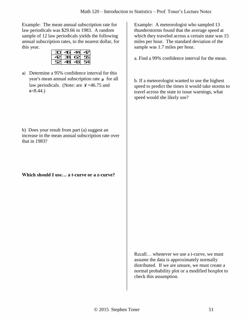
Example: The mean annual subscription rate for

law periodicals was $29.66 in 1983. A random

sample of 12 law periodicals yields the following

annual subscription rates, to the nearest dollar, for

this year.

30 46 44 47

42 38 62 55

52 48 43 54

a) Determine a 95% confidence interval for this

year's mean annual subscription rate for all

law periodicals. (Note: are x =46.75 and

s=8.44.)

b) Does your result from part (a) suggest an

increase in the mean annual subscription rate over

that in 1983?

Which should I use… a t-curve or a z-curve?

Example: A meteorologist who sampled 13

thunderstorms found that the average speed at

which they traveled across a certain state was 15

miles per hour. The standard deviation of the

sample was 1.7 miles per hour.

a. Find a 99% confidence interval for the mean.

b. If a meteorologist wanted to use the highest

speed to predict the times it would take storms to

travel across the state to issue warnings, what

speed would she likely use?

Recall… whenever we use a t-curve, we must

assume the data is approximately normally

distributed. If we are unsure, we must create a

normal probability plot or a modified boxplot to

check this assumption.



8.3 Population Proportions

Suppose we wish to know what proportion of a

population has a particular attribute.

Let p = population proportion

p = sample proportion

Formula: px

n

Note that p is a statistic being used to make a

prediction about the population parameter p .

example: If 108 families were sampled to see if

they have a microwave and x=102 responded

"yes," then 102

ˆ108

p .

Suppose a large random sample of size n is to be

taken from a 2-category population with

population proportion p. Then the random

variable p is approximately normally distributed

with p and

p

p p

n

1

Assumptions:

a simple random sample was taken

the population is at least 20 times larger than

the sample

the items in the population are divided into

two categories

the samples must contain at least 10

individuals in each category

The margin of error E for the estimate of p is

given by E=

Z

p p

n 2

1

. (It is equal to

half of the confidence interval.)

example: Studies are performed to determine the

percentage of the nation's 10 million asthmatics

who are allergic to sulfites. In a recent survey, 38

of 500 randomly selected U.S. asthmatics were

found to be allergic to sulfites.

a) Determine a 95% confidence interval for the

proportion, p, of all U.S. asthmatics who are

allergic to sulfites.

b) Interpret your results from part (a).

Sample Size:

To determine the proper sample size to match the

margin of error with the confidence level, first

determine whether p (or an estimate for p ) is

known or not. Use n= p p

Z

E

12

2

, then

round up to the nearest integer when p is known.

Use n=0 252

2

.

Z

E

, rounded up to the nearest

integer when a guess for p is unknown.

Graph of p versus pp ˆ1ˆ



example: Referring to the previous example

(U.S. asthmatics),

a) Determine the margin of error for the estimate

of p.

b) Obtain a sample size that will ensure a margin

of error of at most 0.01 for a 95% confidence

interval without making a guess for the

observed value of p .

c) Find a 95% confidence interval for p if for a

sample of the size determined in part (b), the

proportion of asthmatics allergic to sulfites is

0.071.

d) Determine the margin of error for the estimate

in part (c) and compare it to the margin of

error specified in part (b).

Example: 35% of adults in America eat pizza at

least once per week. A random sample of 250

adults in a medium-size college town were

surveyed, and it was found that 110 eat pizza at

least once per week. Estimate the true proportion

of American adults who eat pizza at least once

per week with 90% confidence and comment on

your results.

A recent study indicated that 29% of the women

of the 100 women over age 55 in a study were

widows.

a. How large a sample must you take to be 90%

confident that the estimate is within 0.05 of the

true proportion of women over age 55 who are

widows?

b. If no estimate of the sample proportion is

available, how large should the sample be?

7.1 the standard normal curve standardizing normal ...the "bell-shaped" curve, or normal...

Documents