Economics 314 Coursebook, 2017 Jeffrey Parker

8 BASIC MACROECONOMIC MODELS: THE

MULTIPLIER, QUANTITY THEORY, IS/LM, AND AGGREGATE SUPPLY AND DEMAND

Chapter 8 Contents

A. Topics and Tools ............................................................................. 2 B. The Quantity Theory of Money .......................................................... 3

Money supply and demand ........................................................................................... 3 Equation of exchange .................................................................................................... 4 The quantity theory ...................................................................................................... 5

C. Income, Expenditures, and the Keynesian Multiplier ............................... 6 Keynes and the classics .................................................................................................. 6 The multiplier process in math terms .............................................................................. 8 More direct derivation: Solving the model ....................................................................... 9 Graphical analysis of the income-expenditure model ...................................................... 10

D. The IS/LM Model........................................................................... 12 The structure of the model ........................................................................................... 13 Expenditure equilibrium and the IS curve ..................................................................... 14 Asset equilibrium and the LM curve ............................................................................. 15 Equilibrium in the IS/LM model ................................................................................ 18

E. Aggregate Demand and Supply .......................................................... 19 Output and prices ....................................................................................................... 20 Levels or growth rates? ................................................................................................ 20 Aggregate supply and the natural level of output ............................................................ 22 Upward-sloping aggregate supply ................................................................................. 23 A fixed point on the short-run AS curve ........................................................................ 24 Aggregate demand ...................................................................................................... 26 The IS/LM model and aggregate demand .................................................................... 27 The quantity theory and aggregate demand .................................................................. 29 Static equilibrium ....................................................................................................... 30 Shocks to aggregate demand ........................................................................................ 31 Shocks to aggregate supply .......................................................................................... 32

F. Dynamic Equilibrium in the AS/AD Model .......................................... 34 Why the AS curve shifts over time ................................................................................ 34

1 – 2

Why the AD curve shifts over time ............................................................................... 34 Equilibrium with growth and inflation ......................................................................... 35 A “growth recession” .................................................................................................. 37

G. A Preview of Romer’s Text from the Perspective of Aggregate Supply/Demand ................................................................................. 38

Growth models ........................................................................................................... 38 Real business cycles ..................................................................................................... 39 The IS/LM model ..................................................................................................... 39

H. Suggestions for Further Reading ........................................................ 40 I. Works Cited in Text ......................................................................... 40

A. Topics and Tools

Several basic macroeconomic models are staples of introductory and intermediate macroeconomics textbooks. Romer’s text does not cover this basic material, which most graduate students would be expected to know from their undergraduate courses. This chapter attempts to fill that gap, providing brief and simple expositions of these models as background for subsequent sections of the course. The first model is the quantity theory of money, which predates Keynes and is a simple mechanism for adding a monetary asset into the model. The second is the Keynesian multiplier, which was arguably the most important policy conclusion of Keynes’s General Theory. We then consider the IS/LM model developed by Hicks (1937), which became the standard exposition of Keynesian, aggregate-demand-based macroeconomics in the 1950s and 1960s. Finally, we consider a simple model of ag-gregate demand and aggregate supply. These models are not built on rigorous foundations of well-specified maximization behavior; hence they have largely been abandoned by today’s academic macroecono-mists. However, they are of interest to us for two main reasons. First, they are an im-portant part of the historical evolution of macroeconomics and are part of the basic lexicon of macroeconomists. Second, purely because of their simplicity, these models are sometimes more useful than more elaborate micro-based models for explaining changes in the macroeconomy.

1 – 3

B. The Quantity Theory of Money

The quantity theory of money, or just “quantity theory” for short, was central to the “classical economics” paradigm against which the Keynesian revolution rebelled. Among the most cited expositions of classical macroeconomics and the quantity the-ory are those of Irving Fisher (1913) and A. C. Pigou (1933). On the micro side, classical economics developed the model we now know as com-petitive general-equilibrium theory. This theory uses supply and demand curves for individual commodities and resources to predict the equilibrium quantities and relative prices of everything, including all goods and services, labor, and capital resources, in-cluding future goods as well as present ones. There was one notable missing link on this classical microeconomic model; it did not explain how the overall general price level was determined. In other words, it could explain using demand and supply curves whether asparagus should be expensive or cheap relative to other goods—the “relative price” of asparagus—but it could not tie down that price in absolute dollar terms. What was required to fill in this missing link was to determine the value, or price, of money in terms of goods, which is the reciprocal of the price of goods in terms of money, which we call the “general price level.” Given that supply and demand analy-sis determined the value of all of the other goods in the model, it made sense to con-sider the supply of and demand for money as determinants of the value of money. Before proceeding to discuss the supply and demand for money, we must clarify

that money is a stock rather than a flow.1 When we talk about the “supply of money”

we are talking about the current available stock of whatever monetary assets are used in the economy. For example, if money is just dollar bills, the supply of money is the total number of dollar bills that are held in the economy at a moment of time: add up the number in your wallet and the wallets and cash drawers of all of the households and firms in the economy. Similarly, the demand for money is the amount of its total stock of wealth that households and firms want to hold in the form of the monetary asset. When thinking of the demand for money we should think in terms of our desire to hold cash vs. other kinds of assets such as bonds, stock, or physical assets.

Money supply and demand The quantity theory treats the supply of money as exogenous. In the gold-standard era (when the model was created), the stock of money mainly depended on the quan-tity of monetary gold circulating in the economy. The monetary gold stock changed

1 In later chapters we shall examine in more detail the characteristics of the assets that we clas-

sify as money and what assets have those characteristics.

1 – 4

largely as a result of mining activity that created new gold or of imbalances in foreign trade that led to gold leaving or entering the economy from abroad. In modern econ-omies, we think of the stock of monetary assets as being determined by a process driven by a central bank that, as an initial approximation, can be considered to set the money supply exogenously. The demand for money is decided by the households and firms that hold it, bal-ancing the costs and benefits of holding money against those of other assets. We dis-cussed the demand for money in detail in the previous chapter. In the basic formula-tion of the quantity theory money demand is assumed to be mathematically propor-tional to transaction volume. More sophisticated models also incorporate the cost of holding money, of which the main component is the forgone interest or other return that could be earned on nonmonetary assets. We will defer discussion of these models until later.

Equation of exchange The central mathematical expression of the quantity theory is the equation of ex-change: MV = PY. Both sides measure total nominal (dollar) transactions in the econ-omy, so the equation is a tautology that must always hold. To make it a theory, we add assumptions about the causal relationships among the variables. The right-hand side of the equation PY is the product of the price level and real GDP, which is just nominal GDP. This is the dollar value of all final goods and ser-vices produced and purchased in the economy during the year—the dollar value of all final transactions. The left-hand side is the product of the money stock, which is assumed to be ex-ogenous, and the “income velocity” of money V. Income velocity is the number of times that the average dollar in the economy is spent on final goods and services during

a year.2 The product of the number of dollars times the number of times the average

dollar is spent during the year must equal the total volume of dollar spending, so MV always equals PY by construction. Because M is a stock and PY is a flow, velocity must be doing something to trans-late between stocks and flows. To see how this works, consider the units in which the variables are measured. Y is a flow of goods per year and P is the price level measured in dollars per good, so the measurement unit of their product is dollars per year. The money stock M is measured in dollars, with no time unit at all. Velocity is a number

2 We must make sure that the collection of transactions that are counted on the left-hand side

matches the collection counted on the right. Because Y includes only final goods and services, we use income velocity on the left rather than the more intuitive “transactions velocity,” which would count monetary expenditures on intermediate goods as well as final goods.

1 – 5

of times per year, so its units are 1/years. Multiplying M by V converts it from a stock to a flow with units of dollars per year, matching the units of the right-hand side. Velocity reflects (inversely) people’s demand for money, given their transaction flow. A higher velocity corresponds to making a given quantity of money perform more transactions, so high velocity reflects a low desire to hold money. We can repre-sent the nominal demand for money in the equation of exchange as

d PYM

V= , (1)

so the equation of exchange shows how velocity and transactions volume work to de-termine how much money people want to hold.

The quantity theory The quantity theory makes assumptions about how the four variables in the equa-tion of exchange are determined. The supply of money M is assumed to be exoge-nously determined by the central bank (or by the gold stock in classical times). Real output Y is assumed to be the aggregation of the quantities of individual goods and services determined by the interaction of demand and supply equations in individ-ual markets. This is the “natural” or “potential” level of output in the economy, a concept that we shall use frequently in this course. In contrast to Keynes’s assumption that real output is determined wholly by aggregate demand (which we introduce later in this chapter), the quantity theory assumes that only aggregate-supply factors matter; real output does not depend in any important way on the price level, the money supply, or velocity. We established in the previous chapter that the demand for money should depend on the costs and benefits of holding money. The benefits are facilitation of transac-tions, which is represented by the PY expression in the numerator of equation (1). Any effects of the cost of money holding, such as the forgone interest on other assets, would have to affect money demand by changing velocity in this formulation. In the simple form of the quantity theory, classical economists treated V as a con-stant. They recognized that different economies might have different monetary insti-tutions that would allow them to use money more or less efficiently and lead to a higher or lower V (consider ATMs in the modern context). But they argued that these institutional characteristics of the monetary system were unlikely to change easily or quickly, so they claimed that V could reasonably be assumed not to change in response to shocks such as changes in the money supply. Having provided theories for how M, Y, and V are determined, all that remains is to consider P, the general price level. The quantity theory asserts that P is determined by the equation of exchange, with M, Y, and V taking on given values as discussed

1 – 6

above. Thus, the quantity theory is a causal version of the equation of exchange, stat-ing that P will be

MV

PY

= (2)

with the variables on the right-hand side all being determined independently. The principal implication of the quantity theory is that money is neutral, which means that changes in the nominal quantity of money lead to proportional increases in prices (as well as wages, nominal exchange rates, and any other dollar magnitudes in the economy) and leave all “real” variables such as output and employment (and the real wage, measured in terms of purchasing power) unchanged. In terms of elastic-ities, the elasticity of the price level with respect to the money supply is one and the elasticity of output with respect to the money supply is zero.

C. Income, Expenditures, and the Keynesian Multiplier

Keynes and the classics The quantity theory offered no clue about why high unemployment might persist as it did during the Great Depression. Classical economists could only assert that ad-justment to the inevitable full-employment equilibrium was very slow. The quantity theory is also very pessimistic about the prospect that government policies might mit-igate the slump in output. If money is neutral, as their theory asserts, then monetary policy is useless because it does not affect real output. In undergraduate macroeconomics courses that begin with the study of short-run fluctuations, the usual starting point is the income-expenditure model that leads to the basic Keynesian expenditure multiplier. This model achieved fame through its expo-sition in Chapter 10 of Keynes’s General Theory, although Keynes points out that the idea of the multiplier originates with R. F. Kahn (1931). Kahn and Keynes were writ-ing in the midst of the Great Depression, when major economies had extensive unu-tilized productive capacity and prices were falling. This led to a set of assumptions that are unreasonable when applied to a “normal” economy near full employment, but that are more realistic in the context in which they were proposed. The crucial difference between the Keynes’s income-expenditure model and the quantity theory lies in how output is determined. In the former, desired aggregate spending (aggregate demand) is the sole determinant of output—firms in the aggregate

1 – 7

will produce whatever amount they can sell. In the latter, production levels are deter-mined by the economy’s resources of labor and capital and by the technological knowledge that is available for using them in production—there is no role for “aggre-gate demand” because aggregate supply is assumed to be perfectly inelastic. The central point in Keynes’s analysis is the importance of what he called “effec-tive demand,” and we now call aggregate demand. His model assumes that the econ-omy’s real output is determined principally (or in simple versions, solely) by the quan-tity of goods and services that people want to buy rather than by the economy’s capac-ity to produce. Any increase in desired expenditures is assumed to lead to an increase

in firms’ production, but not to any increase in prices.3 This assumption is plausible

for a depression economy, in a situation with high levels of unemployed labor and underutilized plant capacity. But it would not be appropriate for an economy operating near or above capacity. Modern macroeconomic models recognize that neither a perfectly elastic nor a perfectly inelastic aggregate-supply curve explains the economy well. As we will ex-amine below in this chapter, and in great detail in those that follow, modern macroe-conomic models typically feature an upward-sloping short-run aggregate-supply curve, allowing aggregate demand a role—but not the sole role—in determining the amount produced in the short run. But the long-run aggregate-supply curve is usually assumed to be perfectly inelastic: in the long run, the quantity theory is approximately correct, money is neutral, and monetary and fiscal policy do not influence aggregate output. Under the assumption of perfectly elastic supply, any increase in spending on do-mestically produced (i.e., not foreign) goods, whether from an increase in business in-vestment, government spending, or net exports, leads to an increase in output. The Keynesian expenditure multiplier recognizes that this expenditure-induced increase in output is simultaneously an increase in the incomes of those who produce the addi-tional goods. Those whose incomes increase can be expected to increase their own spending, leading to a second round of stimulus to output and income. This is, of course, followed by a third round as those who produce goods that are newly de-manded at the second round see rises in their incomes and choose to increase spending as a result, and by further rounds of spending increases ad infinitum. Each successive round of increase in spending is smaller than its predecessor as long as people spend only part of the increase in their incomes. Under simple assump-tions (such as a constant marginal spending share that is less than one), the increments to spending of successive rounds die away to zero and the ultimate increase in output, income, and spending approaches a finite multiple of the original increase in spend-ing—the Keynesian expenditure multiplier.

3 Later in this chapter, we will characterize this assumption as a perfectly elastic short-run ag-

gregate-supply curve.

1 – 8

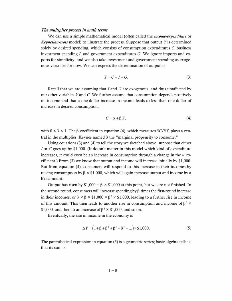
The multiplier process in math terms We can use a simple mathematical model (often called the income-expenditure or Keynesian-cross model) to illustrate the process. Suppose that output Y is determined solely by desired spending, which consists of consumption expenditures C, business investment spending I, and government expenditures G. We ignore imports and ex-ports for simplicity, and we also take investment and government spending as exoge-nous variables for now. We can express the determination of output as .Y C I G= + + (3)

Recall that we are assuming that I and G are exogenous, and thus unaffected by our other variables Y and C. We further assume that consumption depends positively on income and that a one-dollar increase in income leads to less than one dollar of increase in desired consumption. ,C Y= α +β (4)

with 0 < β < 1. The β coefficient in equation (4), which measures ∂C/∂Y, plays a cen-

tral in the multiplier; Keynes named β the “marginal propensity to consume.” Using equations (3) and (4) to tell the story we sketched above, suppose that either I or G goes up by $1,000. (It doesn’t matter in this model which kind of expenditure

increases, it could even be an increase in consumption through a change in the α co-efficient.) From (3) we know that output and income will increase initially by $1,000. But from equation (4), consumers will respond to this increase in their incomes by

raising consumption by β × $1,000, which will again increase output and income by a like amount.

Output has risen by $1,000 + β × $1,000 at this point, but we are not finished. In

the second round, consumers will increase spending by β times the first-round increase

in their incomes, or β × β × $1,000 = β2 × $1,000, leading to a further rise in income

of this amount. This then leads to another rise in consumption and income of β3 ×

$1,000, and then to an increase of β4 × $1,000, and so on. Eventually, the rise in income in the economy is

( )2 3 41 ... $1,000.Y∆ = +β +β +β +β + × (5)

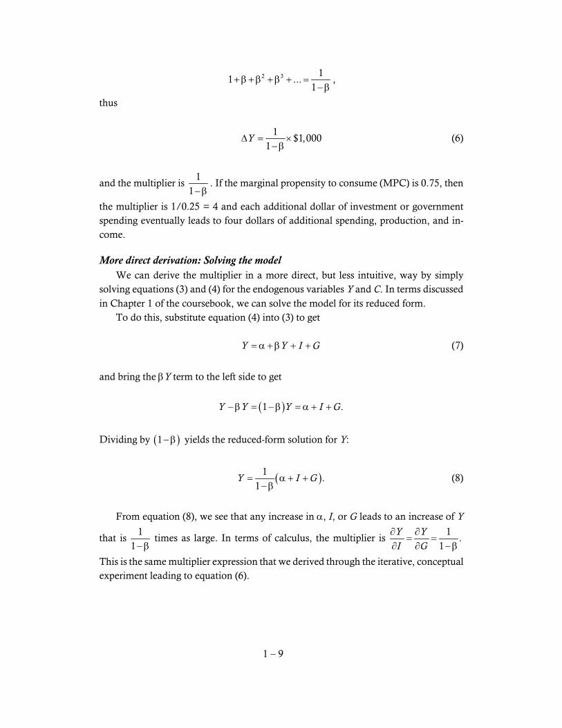
The parenthetical expression in equation (5) is a geometric series; basic algebra tells us that its sum is

1 – 9

2 3 11 ...

1+β +β +β + =

−β,

thus

1

$1,0001

Y∆ = ×−β

(6)

and the multiplier is 1

1−β. If the marginal propensity to consume (MPC) is 0.75, then

the multiplier is 1/0.25 = 4 and each additional dollar of investment or government spending eventually leads to four dollars of additional spending, production, and in-come.

More direct derivation: Solving the model We can derive the multiplier in a more direct, but less intuitive, way by simply solving equations (3) and (4) for the endogenous variables Y and C. In terms discussed in Chapter 1 of the coursebook, we can solve the model for its reduced form. To do this, substitute equation (4) into (3) to get Y Y I G= α +β + + (7)

and bring the βY term to the left side to get

( )1 .Y Y Y I G−β = −β = α + +

Dividing by ( )1−β yields the reduced-form solution for Y:

( )1.

1Y I G= α + +

−β (8)

From equation (8), we see that any increase in α, I, or G leads to an increase of Y

that is 1

1−β times as large. In terms of calculus, the multiplier is

1.

1Y YI G

∂ ∂= =

∂ ∂ −β

This is the same multiplier expression that we derived through the iterative, conceptual experiment leading to equation (6).

1 – 10

Graphical analysis of the income-expenditure model Introductory macroeconomics textbooks often describe the income-expenditure model and the multiplier using a graph with desired expenditures on the vertical axis and income on the horizontal axis. From equation (7), desired expenditures are an increasing linear function of income, as shown by the curve labeled E in Figure 1. The model is in equilibrium when desired expenditures equal income, which hap-pens on the line through the origin with slope of one—the 45-degree line in Figure 1. Equilibrium thus occurs where the desired-expenditure line intersects the 45-degree line at income level Y*. This diagram is often called the “Keynesian cross.”

Figure 1. Income-expenditure model equilibrium

To see that the multiplier is greater than one, consider the effect on equilibrium income of an upward shift in the E curve, such as would occur if investment or gov-ernment spending were to rise. Figure 2 shows the effect of a small increase in govern-

ment spending, represented by the small arrow marked ∆G. The increase in govern-ment spending shifts the desired expenditure curve parallel upward by that amount, as

shown by the E′ curve.

The upward shift of amount ∆G in the expenditure curve raises the equilibrium

level of income from Y* to Y′, an amount shown by the ∆Y arrow in Figure 2. It is

Income

Desired Expenditures

45-degree line

E

Y*

Y*

1 – 11

evident that the change in income is much larger than the original change in govern-

ment spending because of the multiplier. The ratio of the length of the ∆Y arrow to the

∆G arrow is the expenditure multiplier.

Figure 2. Keynesian multiplier

Before leaving the income-expenditure model, it is important to reiterate both its implications and its limitations. In an economic environment such as the Great De-pression with many unemployed workers and extensive idle plant capacity, producers are likely to respond to increases in demand by raising output not price. In this setting, the multiplier analysis shows that an exogenous stimulus to expenditures can lead to a magnified effect on GDP. This is the argument behind using fiscal policy—some combination of increases in government spending and reductions in taxes to increase consumption—to combat economic slumps. It was this analysis that underlay the “stimulus package” (formally, the American Recovery and Reinvestment Act of 2009) that was enacted in February 2009 to mitigate the adverse effects of the financial crisis on the macroeconomy. However, the income-expenditure model makes two crucial assumptions that are unlikely to hold when the economy is near full employment. First, we must assume that the increase in government spending does not displace any private spending. As-suming that taxes are not raised (which would in itself probably offset much of the stimulus), the increase in spending is likely financed by raising government borrowing.

Income

Desired Expenditures

45-degree line

E

Y*

Y*

E′

Y′

Y′

∆G

∆Y

1 – 12

Depending on conditions in financial markets, this increase in borrowing might raise interest rates, making it more expensive for private firms to borrow to build factories and for households to borrow for purchases of cars and houses. This effect is modeled in the IS/LM model that we discuss later in this chapter. If private spending goes down when government spending rises, then the net increase in spending may be much smaller, reducing the stimulative effect on output. However, in both the Great Depres-sion and the 2009 stimulus, interest rates were very low and did not seem to rise when government spending rose. The second crucial assumption is that firms respond to increased demand solely by raising output. We argued above that this assumption was reasonable (at least as a first approximation) during the Great Depression, but firms that are near their optimal production capacity are likely to respond to a rise in demand by increasing their prices more than by increasing output. If this happens, then the stimulative effect of increased government spending will be dissipated on price increases rather than expansion of real output. We shall see this later in this chapter when we discuss the slope of the aggregate-supply curve and its effect on the responses of output and prices to changes in aggregate demand. In the recent recession, the magnitude of fiscal-policy multipliers was a controver-sial and heavily studied topic. Three articles in the September 2011 issue of Journal of Economic Literature provide a good sample from different ideological and methodolog-ical perspectives: Taylor (2011), Parker (2011), and Ramey (2011). Expenditure multipliers are also often used by urban economists to analyze the secondary effects of activities that boost local spending, such as a large public-works project, the movement into the area of a large new plant, or the creation, attraction, or retention of a new professional sports franchise. In each case, expenditures by those who earn income from the initial activity lead to secondary income effects. However, to evaluate local effects, one must be careful to restrict the MPC to include only income-induced expenditures on local goods and services.

D. The IS/LM Model

The multiplier analysis of the income-expenditure model gained widespread ac-ceptance after its publication in the early 1930s. Its explanation of the causes of and potential solution to the Great Depression resonated with those who despaired at the laissez-faire mantra of classical economics. But even its proponents recognized that sev-eral mitigating factors would cause the actual effect of an increase in expenditures to be smaller than the simple multiplier suggests.

1 – 13

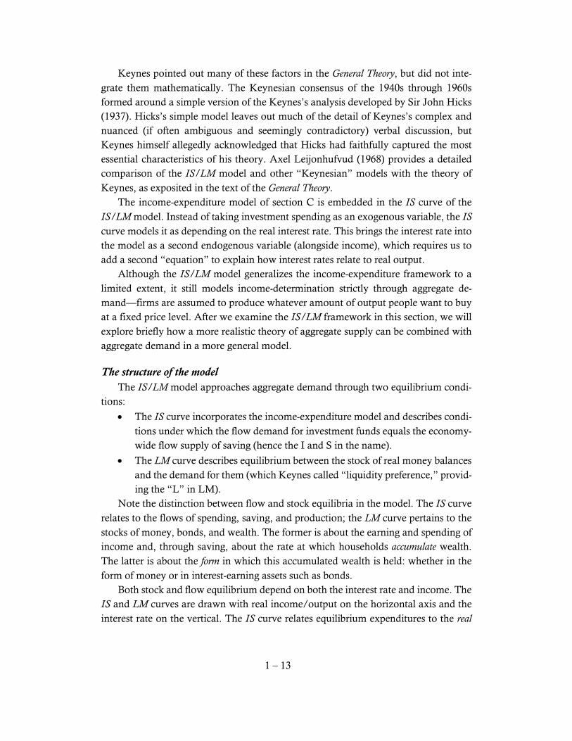
Keynes pointed out many of these factors in the General Theory, but did not inte-grate them mathematically. The Keynesian consensus of the 1940s through 1960s formed around a simple version of the Keynes’s analysis developed by Sir John Hicks (1937). Hicks’s simple model leaves out much of the detail of Keynes’s complex and nuanced (if often ambiguous and seemingly contradictory) verbal discussion, but Keynes himself allegedly acknowledged that Hicks had faithfully captured the most essential characteristics of his theory. Axel Leijonhufvud (1968) provides a detailed comparison of the IS/LM model and other “Keynesian” models with the theory of Keynes, as exposited in the text of the General Theory. The income-expenditure model of section C is embedded in the IS curve of the IS/LM model. Instead of taking investment spending as an exogenous variable, the IS curve models it as depending on the real interest rate. This brings the interest rate into the model as a second endogenous variable (alongside income), which requires us to add a second “equation” to explain how interest rates relate to real output. Although the IS/LM model generalizes the income-expenditure framework to a limited extent, it still models income-determination strictly through aggregate de-mand—firms are assumed to produce whatever amount of output people want to buy at a fixed price level. After we examine the IS/LM framework in this section, we will explore briefly how a more realistic theory of aggregate supply can be combined with aggregate demand in a more general model.

The structure of the model The IS/LM model approaches aggregate demand through two equilibrium condi-tions:

• The IS curve incorporates the income-expenditure model and describes condi-tions under which the flow demand for investment funds equals the economy-wide flow supply of saving (hence the I and S in the name).

• The LM curve describes equilibrium between the stock of real money balances and the demand for them (which Keynes called “liquidity preference,” provid-ing the “L” in LM).

Note the distinction between flow and stock equilibria in the model. The IS curve relates to the flows of spending, saving, and production; the LM curve pertains to the stocks of money, bonds, and wealth. The former is about the earning and spending of income and, through saving, about the rate at which households accumulate wealth. The latter is about the form in which this accumulated wealth is held: whether in the form of money or in interest-earning assets such as bonds. Both stock and flow equilibrium depend on both the interest rate and income. The IS and LM curves are drawn with real income/output on the horizontal axis and the interest rate on the vertical. The IS curve relates equilibrium expenditures to the real

1 – 14

interest rate; the LM curve describes equilibrium in asset holding in terms of the nomi-nal interest rate. One can put either the real or nominal interest rate on the vertical axis, but in either case one of the curves must be adjusted to account for the expected rate of inflation—the difference between the nominal and real interest rates. There is no standard among textbooks about which convention to use; many inferior texts ig-nore the distinction entirely. In this analysis, we will use the real interest rate r on the vertical axis.

Expenditure equilibrium and the IS curve The IS curve generalizes the income-expenditure model by considering the ways in which other variables, notably including the real interest rate, affect the desired-expenditure curve E in Figure 1. In general, anything (other than income itself) that causes desired expenditures to change will shift the E curve upward or downward and cause a (multiplied) change in equilibrium spending. The real interest rate r is one of the variables that affects desired expenditures, so the equilibrium level of income in the income-expenditure model depends on the level of r. Without (for now) deriving the theory from rigorous individual-choice founda-tions, it is reasonable to assert that both the consumption and investment components of desired expenditures are likely to be negatively related to real interest rates. A higher real interest rate increases the reward to saving, leading to a substitution effect away from current consumption spending (and toward future consumption), reducing C. Purchases of consumer durables, which are often financed explicitly by borrowing, are especially likely to be interest-sensitive because people will easily recognize the effect of a higher interest rate on their monthly loan payments. The real interest rate also measures the cost (either directly, if the firm borrows, or as an implicit opportunity cost) of business investment in plant and equipment, so an increase in interest rates is likely to lower firms’ desired spending I on new capital goods. A higher real interest rate implies lower desired expenditures, so it shifts the de-sired-expenditure curve in the income-expenditure diagram downward, leading to a (multiplied) contraction of aggregate demand and GDP. The downward-sloping curve that plots the effect of the real interest rate (on the vertical axis) on the level of equilib-

rium income (on the horizontal axis) is called the IS curve.4

4 Hicks’s derivation of the IS curve used investment = saving as the condition for equilibrium;

we have used income = expenditures. Ignoring government, Y = C + I is our condition for income = expenditures. Since households allocate their current income between consumption and saving, Y = C + S. Setting these two equations equal to one another, equilibrium between expenditures and income can also be written as I = S, which is the form used by Hicks, leading him to call the resulting curve the IS curve.

1 – 15

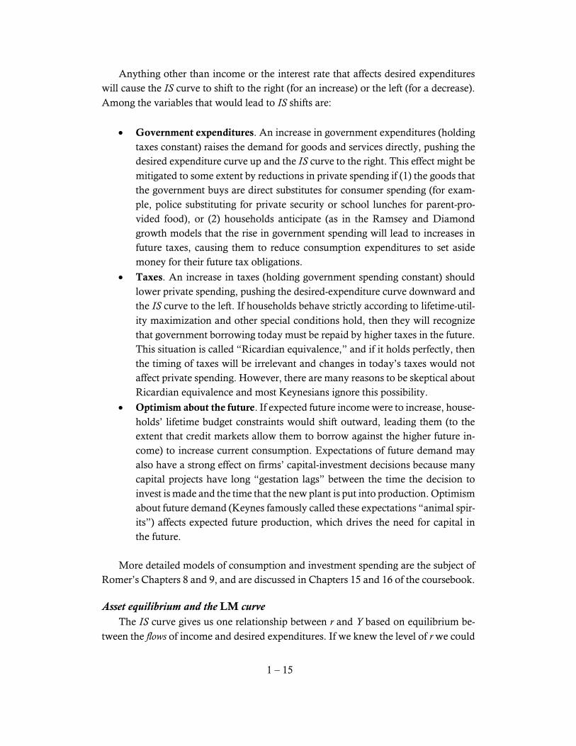
Anything other than income or the interest rate that affects desired expenditures will cause the IS curve to shift to the right (for an increase) or the left (for a decrease). Among the variables that would lead to IS shifts are:

• Government expenditures. An increase in government expenditures (holding taxes constant) raises the demand for goods and services directly, pushing the desired expenditure curve up and the IS curve to the right. This effect might be mitigated to some extent by reductions in private spending if (1) the goods that the government buys are direct substitutes for consumer spending (for exam-ple, police substituting for private security or school lunches for parent-pro-vided food), or (2) households anticipate (as in the Ramsey and Diamond growth models that the rise in government spending will lead to increases in future taxes, causing them to reduce consumption expenditures to set aside money for their future tax obligations.

• Taxes. An increase in taxes (holding government spending constant) should lower private spending, pushing the desired-expenditure curve downward and the IS curve to the left. If households behave strictly according to lifetime-util-ity maximization and other special conditions hold, then they will recognize that government borrowing today must be repaid by higher taxes in the future. This situation is called “Ricardian equivalence,” and if it holds perfectly, then the timing of taxes will be irrelevant and changes in today’s taxes would not affect private spending. However, there are many reasons to be skeptical about Ricardian equivalence and most Keynesians ignore this possibility.

• Optimism about the future. If expected future income were to increase, house-holds’ lifetime budget constraints would shift outward, leading them (to the extent that credit markets allow them to borrow against the higher future in-come) to increase current consumption. Expectations of future demand may also have a strong effect on firms’ capital-investment decisions because many capital projects have long “gestation lags” between the time the decision to invest is made and the time that the new plant is put into production. Optimism about future demand (Keynes famously called these expectations “animal spir-its”) affects expected future production, which drives the need for capital in the future.

More detailed models of consumption and investment spending are the subject of Romer’s Chapters 8 and 9, and are discussed in Chapters 15 and 16 of the coursebook.

Asset equilibrium and the LM curve The IS curve gives us one relationship between r and Y based on equilibrium be-tween the flows of income and desired expenditures. If we knew the level of r we could

1 – 16

use the IS curve to figure out what the equilibrium Y must be, or vice versa. But in order to determine the levels of both variables, we need a second equilibrium relationship. We seek the needed relationship by examining the equilibrium between the stock sup-plies of monetary and non-monetary assets and the demand for these assets. The traditional way to characterize the asset-equilibrium relationship is the LM curve, describing the conditions leading the quantity of money demanded by house-holds and firms to equal the quantity supplied by the central bank and the financial system. Since the demand for money depends on the interest rate (negatively) and in-come (positively), there are many alternative combinations of r and Y for which the demand will equal any given level of money supply. This upward-sloping collection of (Y, r) pairs is the LM curve. The LM analysis was developed to describe a financial system in which the time path of the money stock is exogenously determined by the institutions of monetary supply, either through the rules of the gold standard or by the decisions of a central bank that sets a target level or growth rate for the money stock. Under such a regime, the short-term interest rate adjusts in order to balance endogenous money demand with the exogenous quantity supplied. The IS/LM analysis has fallen out of favor—even among Keynesian macroecon-omists who do not object to the absence of microfoundations—because most modern central banks no longer set monetary policy according to money-supply or money-growth targets. Instead, most now follow policies that target a specific short-term in-terest rate and allow the money supply to adjust to whatever level achieves balances

asset markets at the desired interest-rate target.5 This makes the money supply endog-

enous and suggests that we should model the central bank’s decision rule for setting the interest rate as our second curve. We shall study a variant of this kind, the IS/MP model, when we get to Romer’s Chapter 6. For now, we explore the historically im-portant IS/LM model. If the income velocity of money is constant, as we assumed in the quantity theory, then the nominal demand for money is given by equation (1). But Keynes (and some classical economists before him) noted that the interest rate should affect the share of people’s wealth that they want to hold in the form of money. In the simplest setting,

bonds (and other assets) bear interest at real rate r and nominal rate i = r + π, where π is the rate of inflation (actual or expected, we do not distinguish between them here for simplicity). Money—think gold or currency here—bears zero nominal interest, and

its real return is –π; money’s real value depreciates at the rate of inflation. The difference between the rate of interest on bonds and the rate of interest on money is the opportunity cost of holding wealth as money rather than as bonds. This

5 The Federal Reserve Board in the United States last followed a strict monetary rule between

1979 and 1982. Since then, interest-rate targets have been more important.

1 – 17

difference equals the nominal rate of interest on bonds.6 A higher nominal interest rate

should cause households to economize on money holdings (choosing to shift wealth into bonds), turning over their dollars more quickly in order to make their needed transactions. In other words, when the interest rate rises people will increase their ve-locity of money. We can incorporate this effect into equation (1) very simply:

( )

d PYM

V r=

+ π, (9)

where ( )V r + π is velocity written as a function of the nominal interest rate with the

assumption that ( ) 0V r′ + π > . Equation (9) is usually rewritten in terms of the de-

mand for real money balances M/P. Dividing both sides by P yields

( ) ( ), ,

dM YL Y r

P V r= ≡ + π

+ π (10)

where the L function is Keynes’s “liquidity preference” function. From equation (10) to the equation for the LM curve is a small step: setting the amount of real money that people want to hold (from (10)) equal to the exogenous real supply of money provided by the central bank (or the stock of monetary gold). Taking M s as exogenous and assuming that P is also given—because we are still assuming that producers supply output perfectly elastically at the given price level—the LM curve is given by

( )

.sM Y

P V r=

+ π (11)

In equation (11), π is the underlying or expected rate of inflation. We take this variable to be exogenous as well, so the only two endogenous variables in (11) are Y and r. This, then, is the second equation that we require to work alongside the IS curve to determine the equilibrium values of Y and r. Whereas the IS curve was shown to slope downward, we can easily demonstrate that the LM curve must slope upward. Suppose that income in the economy were to

6 The difference between the nominal returns on bonds and money is i – 0 = i. The difference

between the real returns is r – (–π) = i – π + π = i. Thus we get the same answer whether we

calculate the difference between bonds and money in nominal returns or real returns.

1 – 18

increase. This would mean more real transactions and would induce people to want to hold greater money balances. (The right-hand side of (11) would increase.) With a given supply of money and a given price level, the only way to rebalance equation (11) would be through a change in r. To offset the increase in money demand arising from higher income, the interest rate would have to increase in order to raise velocity so that the denominator of (11) rises to match the increase in the numerator. Thus, the LM curve must slope upward: other things held constant, an increase in real income re-quires an increase in the interest rate in order to rebalance money demand with money supply.

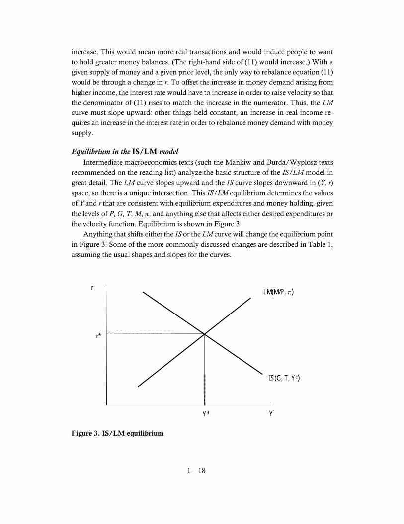
Equilibrium in the IS/LM model Intermediate macroeconomics texts (such the Mankiw and Burda/Wyplosz texts recommended on the reading list) analyze the basic structure of the IS/LM model in great detail. The LM curve slopes upward and the IS curve slopes downward in (Y, r) space, so there is a unique intersection. This IS/LM equilibrium determines the values of Y and r that are consistent with equilibrium expenditures and money holding, given

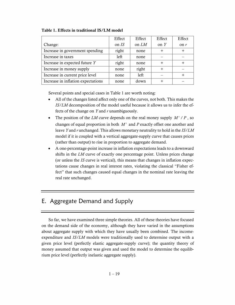
the levels of P, G, T, M, π, and anything else that affects either desired expenditures or the velocity function. Equilibrium is shown in Figure 3. Anything that shifts either the IS or the LM curve will change the equilibrium point in Figure 3. Some of the more commonly discussed changes are described in Table 1, assuming the usual shapes and slopes for the curves.

Figure 3. IS/LM equilibrium

r

Y

IS(G, T, Ye)

LM(M/P, π)

Yd

r*

1 – 19

Table 1. Effects in traditional IS/LM model

Change: Effect on IS

Effect on LM

Effect on Y

Effect on r

Increase in government spending right none + +

Increase in taxes left none – –

Increase in expected future Y right none + +

Increase in money supply none right + –

Increase in current price level none left – +

Increase in inflation expectations none down + –

Several points and special cases in Table 1 are worth noting:

• All of the changes listed affect only one of the curves, not both. This makes the IS/LM decomposition of the model useful because it allows us to infer the ef-fects of the change on Y and r unambiguously.

• The position of the LM curve depends on the real money supply /sM P , so

changes of equal proportion in both sM and P exactly offset one another and leave Y and r unchanged. This allows monetary neutrality to hold in the IS/LM model if it is coupled with a vertical aggregate-supply curve that causes prices (rather than output) to rise in proportion to aggregate demand.

• A one-percentage-point increase in inflation expectations leads to a downward shifts in the LM curve of exactly one percentage point. Unless prices change (or unless the IS curve is vertical), this means that changes in inflation expec-tations cause changes in real interest rates, violating the classical “Fisher ef-fect” that such changes caused equal changes in the nominal rate leaving the real rate unchanged.

E. Aggregate Demand and Supply

So far, we have examined three simple theories. All of these theories have focused on the demand side of the economy, although they have varied in the assumptions about aggregate supply with which they have usually been combined. The income-expenditure and IS/LM models were traditionally used to determine output with a given price level (perfectly elastic aggregate-supply curve); the quantity theory of money assumed that output was given and used the model to determine the equilib-rium price level (perfectly inelastic aggregate supply).

1 – 20

Whether we think of these models as determining Y given P or determining P given Y, all three are basically models of aggregate demand. In this section, we combine aggregate demand with aggregate supply to examine the short-run and long-run equi-librium of the macroeconomy.

Output and prices The central endogenous variables in aggregate supply-demand analysis are real output and the general price level. With the assignment of quantity to the horizontal axis and price to the vertical axis, the AS/AD model resembles the familiar supply-demand model of perfect competition. Indeed they are very similar in some ways, however it is extremely important not to push the parallels too far; some properties of the curves and models are very different. There are important differences between the variables Y and P on the axes of the AS/AD model and the familiar quantity and price variables of microeconomics. The quantity variable Y on the horizontal axis of the AS/AD model measures the total output of the economy (real GDP) rather than the physical output of some specific commodity. This leads to important differences in the interpretation of the curves. For example, the demand curve for zucchini slopes downward because consumers will substitute other foods as zucchini get expensive. In the macro model, GDP is all goods,

so there is nothing obvious to substitute for GDP if it gets expensive.7 Thus, in the

macro context we cannot rely on the familiar logic of substitution to motivate the neg-ative slope of the demand curve. The price variable P on the vertical axis is also fundamentally different. In the AS/AD model, price refers to the aggregate price of all goods and services—a price index like the GDP deflator—rather than the relative price of zucchini as in the micro model. Again, this has important implications for the behavior of the curves. An in-crease in all prices may not have any effect on either quantity supplied or quantity demanded if, along with the increase in prices, nominal wages and nominal stocks of assets such as money all increase in equal proportion. This is the familiar principle that the economy exhibits no money illusion—people care only about the real value of things, not about the number of dollars attached to them. If all dollar labels are rede-fined in a proportional way, nothing is more or less expensive than before and there is no reason for real purchases or sales to change.

Levels or growth rates? The simplest form of the AS/AD model puts the level of real GDP on the horizon-tal axis and the level of prices on the vertical axis. Constructing the model in terms of

7 Future goods and foreign goods are possible substitutes. We shall have more to say about such

issues later on.

1 – 21

levels has the advantage of simplicity: the point of intersection defines a unique equi-librium level of output and prices. This is the most common form of the model and is adequate as a momentary snapshot of the macroeconomy. However, modern economies typically exhibit year-to-year growth in real output and year-to-year inflation in the price level rather than levels that stay constant over time. We are often more interested in these rates of change than in the absolute level of GDP and prices. To capture this ongoing behavior in the “levels” version of the AS/AD model, the “equilibrium point” would be moving upward and to the right

over time.8 We can keep the model in terms of levels only if we are willing to discard

the notion of a fixed point of long-run equilibrium and depict the long run as an equi-librium growth/inflation path involving a sequence (or continuum) of points of mo-mentary equilibrium. An alternative modeling strategy is to put the growth rate of output on the hori-zontal axis and/or the inflation rate on the vertical axis, modeling aggregate supply and aggregate demand in terms of percentage changes rather than levels of output and/or prices. By recasting the model in terms of rates of change, the economy may converge to a single point of long-run equilibrium on the graph: one where the growth rate of output and the rate of inflation are constant. However, there are difficulties with casting the model in rates of change as well. Putting the graphical analysis entirely in terms of growth rates means that there is no information on the graph about the level of output. Suppose that last year’s growth rate was unusually low, so the current level of output in the economy is below its long-run growth trend. Conventional macroeconomic theory suggests that such an economy would be expected to grow more quickly in the coming years to recover toward the trend path. On the graph, this means that aggregate supply or aggregate demand (or both) must shift to the right when output is below trend in order to increase growth. In order to incorporate this into the graph, the position of the AD and AS curves must depend on the current level of GDP relative to a benchmark trend. We shall model aggregate supply and demand in levels rather than growth rates. In the simple model that we introduce first, we ignore the tendency of output and prices to grow over the long run. Later in this chapter we will consider the nature of equilibrium behavior with growth and inflation. In competitive microeconomic markets, we use the supply curve and the demand curve to represent, respectively, the behavior of the producers and buyers of a com-modity. By examining the interaction of the two curves and imposing an assumption that the price adjusts to clear the market, we model the equilibrium levels of quantity exchanged and price at the intersection of the two curves.

8 Or downward in the case of deflation and to the left in the case of economic contraction.

1 – 22

The aggregate supply (AS) curve and aggregate demand (AD) curve perform sim-ilar roles for the aggregate macroeconomy. The AS curve summarizes the behavior of the production side of the market: production decisions of firms and activities in the markets for factor inputs. The AD curve summarizes desired purchases in the macro-economy and activities in asset markets that influence demand behavior. Like microeconomic supply curves, the AS curve often slopes upward, though the underlying logic justifying its shape is quite different. The AS curve is horizontal or vertical under some conditions. Unlike microeconomic supply curves, which tend to me more elastic in the long run than in the short run, the AS curve is perfectly inelastic (vertical) in the long run and may be highly elastic (flat) in the short run. The AD curve is generally downward-sloping, just as the microeconomic demand curve is, but again the reasons for the negative slope and the conditions under which it is elastic or ine-lastic are quite different.

Aggregate supply and the natural level of output In microeconomic markets, the positive slope of the supply curve is very natural. If a single good becomes more valuable relative to other goods (i.e., its relative price increases) then firms in the economy will devote more of their productive activity to producing that good, taking resources away from production of other goods. However, this logic does not work the same way in the aggregate macroeconomy. A price increase in the macroeconomy means that the prices of all goods have in-creased. Will this across-the-board price increase impel firms to use more resources to produce goods and services? Maybe, but not necessarily. The benchmark model of neoclassical economics is the perfectly competitive gen-eral-equilibrium (PCGE) model. This is the core model of most microeconomics courses; it is the model that most economists think of first when trying to answer ques-tions about market economies. In the PCGE model, the prices of all goods and inputs are perfectly flexible, all agents are perfectly informed, entry and exit are costless, and no one has any market power. Because buyers and sellers are price-takers, there are well-defined demand and supply curves relating quantities demanded and supplied to price. The quantity of each good and service produced and sold is determined uniquely by the point of intersection of the supply and demand curves. If we were to add up the real value of all of the commodities produced in equilib-rium of the PCGE model, we would obtain a unique value of GDP that reflects the equilibrium amount of production. This unique equilibrium quantity of aggregate out-put in the PCGE model is called the “natural level of output,” or sometimes capacity output or full-employment output. Theorems of welfare economics assure us that the competitive equilibrium allocation of resources (and therefore the amount produced) is Pareto-optimal, given the amounts of factors of production that are available and

1 – 23

the utility-maximizing decisions by laborers about allocating their time between work and leisure. We studied the long-run behavior of natural output in our analysis of growth models. Although natural output is crucially important for macroeconomic theory and pol-icy, it cannot be directly observed or measured. Policymakers must try to estimate the amount that could or should be produced with the current technology and resource endowments in order to know whether current actual output is too low or too high. The natural level of output does not depend on the dollar value of prices in any way. PCGE determines an equilibrium relative price for each commodity. For exam-ple, equilibrium might require that apples be half as expensive as bananas and that the real wage of unskilled labor be 10 apples per hour of work. However, whether this is achieved by apples costing $0.10, bananas $0.20, and a nominal wage of $1.00 or by apples costing $500, bananas costing $1,000, and a nominal wage of $5,000 is com-pletely irrelevant to PCGE model equilibrium. The natural level of output can be achieved at any aggregate price level. If the world behaved according to the PCGE model, real GDP would always equal the natural level of output (Yn) regardless of the nominal level of aggregate prices in the economy. Thus, the assumptions of the PCGE model lead to a vertical aggregate supply curve at Y = Yn.

Upward-sloping aggregate supply Most macroeconomists believe that the PCGE model provides a reasonable ap-proximation of macroeconomic behavior in the “long run,” when prices have time to adjust fully and information becomes fully available, so we usually take the “long-run aggregate supply curve” to be vertical. This implies that output will return to the nat-ural level of output (full employment) in the long run as the equilibrating forces of price movements and information pervasion pull the economy back to the vertical

long-run AS curve.9

However, from a macroeconomic perspective, a vertical AS curve eliminates a lot of interesting possibilities. With a vertical AS, the level of output is always at Yn re-gardless of how the AD curve fluctuates: aggregate demand has no effect on output. Ever since Keynes’s analysis of the Great Depression, most economists have been con-vinced that changes in aggregate demand do affect output, at least temporarily, thus

9 Of course, this assumes that there is no change over time in the determinants of natural output.

If the labor force and capital stock increase and technology improves, then we expect the nat-ural level of output to increase, which will mean that the long-run AS curve is not stationary but instead shifts to the right over time. Thus, the long-run AS curve is “long-run” in the sense that the economy moves toward it in the long run, but not in the sense that it remains stable in the long run.

1 – 24

the vertical AS curve seems like an inadequate description of macroeconomic supply behavior. There are multitudes of theories explaining why the short-run AS curve might slope upward. We will study several of these theories in Romer’s Chapter 6, so there is no need to elaborate the details now. A couple of examples should demonstrate the nature of elastic short-run supply. One possibility is that firms face costs of changing their prices. These costs are often called “menu costs,” as in the costs a restaurant faces when it must reprint menus to reflect changed prices. In that case, if there is upward pressure on nominal prices due to an increase in aggregate demand, some firms may choose not to raise their prices immediately, even if other firms do raise their prices. The relative prices charged by the firms that do not raise prices will be lower than before and they will sell more output as a result. Thus, in the presence of menu costs, some firms will raise prices and others will increase production, so in the aggregate there will be an increase in both

prices and output along an upward-sloping short-run AS curve.10 Note that in this case

we would expect all firms eventually to change their prices (once the old menus wear out), so the justification for an upward-sloping AS curve holds only in the short run. Even with menu costs, we still expect the long-run response to be an increase in all nominal prices with production back at Yn, so the long-run AS curve is vertical. Another possibility is that some of the firm’s nominal costs fail to rise along with prices. For example, if wages are set for a period of time by nominal (fixed-dollar) contracts, an increase in prices (assuming no menu costs) would temporarily raise the firm’s revenues relative to their (labor) costs. This would make it profitable to expand output in the short run while this positive gap between revenues and costs exists. Once again, production increases and prices rise in the short run, so the short-run AS curve slopes upward. However, as in the previous example, we would expect production eventually to return to Yn at the higher price level. In this case, nominal wages would rise when contracts expire and workers whose cost of living has increased bargain for a compensating wage increase. Thus, again, the long-run AS curve is vertical.

A fixed point on the short-run AS curve The two simple aggregate-supply theories sketched above have several character-istics in common. As we shall see later, these characteristics are shared by most short-run aggregate-supply models. Two important characteristics have been stressed above:

10

Note also that we have already strayed from one of the key assumptions of the PCGE model. A price-taking firm in a perfectly competitive market cannot defer its price change; it must charge the market-clearing price. If a few firms kept their prices low in a perfectly competitive market, all buyers would attempt to buy from them, forcing them to increase production dra-matically, which would increase costs and force them to raise prices.

1 – 25

(1) the short-run AS curve slopes upward and (2) the long-run AS curve is vertical at Yn. A third property that connects the short-run and long-run supply curves is less ob-vious: the short-run AS curve passes through the vertical long-run AS (Y = Yn) at the

expected price level. Thus, the point ( ), enY P always lies on the short-run AS curve.

We can explain the logic of this “fixed point” on the AS curve for the two simple models discussed above. With menu costs, we assume that the prices that firms have set for this period (and printed on their menus) are those that they expected to prevail at the time the menus were printed. Thus, if aggregate demand turns out to be as ex-pected, firms will have set the appropriate prices and the economy will be in PCGE with P = Pe and Y = Yn. In the case discussed above, AD is higher than expected, lead-ing to P > Pe and Y > Yn. In the wage-contract model, we assume that firms and workers try to set the nom-inal wage in a way that leads to the PCGE real wage (W/P)*. If they expect the price

level to be Pe, then they set the nominal wage at ( / ) *eW P W P= ⋅ . If aggregate de-

mand is as expected and the price level actually turns out to be Pe, then the actual real

wage will be / ( / ) *eW P W P= and the economy will be in PCGE. If aggregate de-

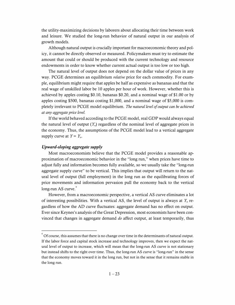
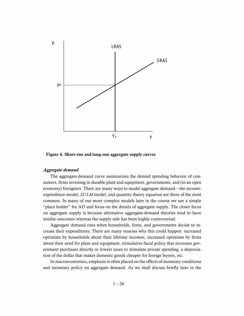
mand is unexpectedly high and the price level exceeds Pe then the real wage will be lower than (W/P)* and firms will expand production. To summarize the conventional properties of aggregate supply, as depicted in Fig-ure 4: The long-run AS curve is vertical at Y = Yn. In the long run, changes in aggre-

gate demand affect only the price level and not the level of real output. The short-run AS curve slopes upward and passes through the point where

Y = Yn and P = Pe. In the short run, increases in aggregate demand lead to in-creases in both price and real output.

1 – 26

Aggregate demand The aggregate-demand curve summarizes the desired spending behavior of con-sumers, firms investing in durable plant and equipment, governments, and (in an open economy) foreigners. There are many ways to model aggregate demand—the income-expenditure model, IS/LM model, and quantity theory equation are three of the most common. In many of our more complex models later in the course we use a simple “place holder” for AD and focus on the details of aggregate supply. The closer focus on aggregate supply is because alternative aggregate-demand theories tend to have similar outcomes whereas the supply side has been highly controversial. Aggregate demand rises when households, firms, and governments decide to in-crease their expenditures. There are many reasons why this could happen: increased optimism by households about their lifetime incomes, increased optimism by firms about their need for plant and equipment, stimulative fiscal policy that increases gov-ernment purchases directly or lowers taxes to stimulate private spending, a deprecia-tion of the dollar that makes domestic goods cheaper for foreign buyers, etc. In macroeconomics, emphasis is often placed on the effects of monetary conditions and monetary policy on aggregate demand. As we shall discuss briefly later in the

P

Y

LRAS

Yn

SRAS

Pe

Figure 4. Short-run and long-run aggregate supply curves

1 – 27

course, an expansionary monetary policy involves the central bank (the Federal Re-serve System in the United States) increasing the supply of monetary assets and, in the process, driving down nominal interest rates on very-short-term loans between finan-cial institutions. The combination of more plentiful monetary assets and lower interest rates tends to stimulate households’ and firms’ desire to spend. In the simplest sense, households that find that they hold additional wealth in the form of monetary assets may simply spend some of it. More subtly, if the reduction in the nominal interbank rate targeted by the central bank diffuses through the market to lower real rates on the interest-bear-ing assets bought and sold by households and firms, then monetary policy may act through an interest-rate channel. Lower (real) interest rates encourage spending by re-ducing the reward to saving and lowering the cost of home mortgages, car loans, and student loans. For businesses, lower real interest rates reduce the cost of borrowing to invest in plants and equipment.

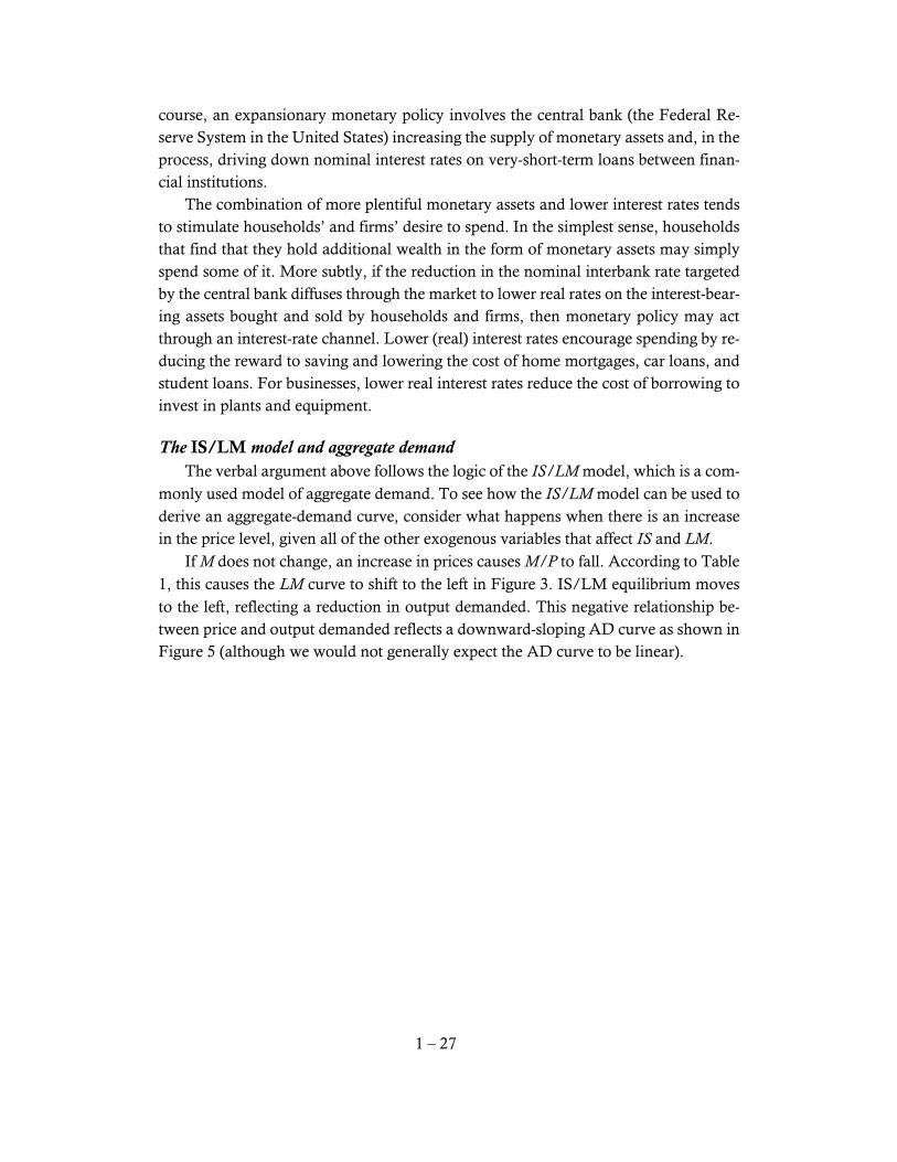
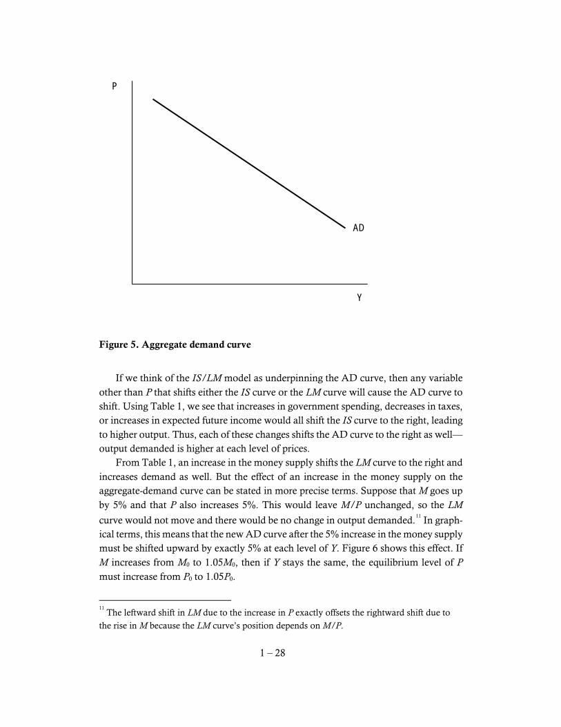
The IS/LM model and aggregate demand The verbal argument above follows the logic of the IS/LM model, which is a com-monly used model of aggregate demand. To see how the IS/LM model can be used to derive an aggregate-demand curve, consider what happens when there is an increase in the price level, given all of the other exogenous variables that affect IS and LM. If M does not change, an increase in prices causes M/P to fall. According to Table 1, this causes the LM curve to shift to the left in Figure 3. IS/LM equilibrium moves to the left, reflecting a reduction in output demanded. This negative relationship be-tween price and output demanded reflects a downward-sloping AD curve as shown in Figure 5 (although we would not generally expect the AD curve to be linear).

1 – 28

P

Y

AD

Figure 5. Aggregate demand curve

If we think of the IS/LM model as underpinning the AD curve, then any variable other than P that shifts either the IS curve or the LM curve will cause the AD curve to shift. Using Table 1, we see that increases in government spending, decreases in taxes, or increases in expected future income would all shift the IS curve to the right, leading to higher output. Thus, each of these changes shifts the AD curve to the right as well—output demanded is higher at each level of prices. From Table 1, an increase in the money supply shifts the LM curve to the right and increases demand as well. But the effect of an increase in the money supply on the aggregate-demand curve can be stated in more precise terms. Suppose that M goes up by 5% and that P also increases 5%. This would leave M/P unchanged, so the LM

curve would not move and there would be no change in output demanded.11 In graph-

ical terms, this means that the new AD curve after the 5% increase in the money supply must be shifted upward by exactly 5% at each level of Y. Figure 6 shows this effect. If M increases from M0 to 1.05M0, then if Y stays the same, the equilibrium level of P must increase from P0 to 1.05P0.

11

The leftward shift in LM due to the increase in P exactly offsets the rightward shift due to

the rise in M because the LM curve’s position depends on M/P.

1 – 29

Figure 6. Effect of 5% increase in money supply on AD

The quantity theory and aggregate demand A simpler alternative to the IS/LM model for underpinning aggregate demand is the quantity theory. If velocity is taken as exogenous, then equation (2) can be viewed as a downward-sloping aggregate-demand curve, expressing P as a function of Y and the two exogenous variables M and V. This curve will be nonlinear (specifically, a rectangular hyperbola) in the levels of P and Y. The quantity-theory AD curve has the same property shown in Figure 6 as the AD curve based on the IS/LM model. A 5% increase in the money supply (or in velocity in this case) leads to a 5% upward shift in the AD curve. Any effect of fiscal policy and other “IS” variables on the quantity-theory-based AD curve is indirect. If changes in government spending, taxes, or expected future incomes do not affect the money supply or velocity, then they will have no effect on aggregate demand. But if we take into account the possible effect of the interest rate on velocity, then these “IS” variables might affect velocity indirectly through their ef-fects on the interest rate. For example, if an increase in government spending raises interest rates in the economy, this would raise the opportunity cost of holding money (vs. bonds), which might increase money velocity as households economize on hold-ing money. The increase in velocity would shift the AD curve up and to the right. When we use the quantity-theory formulation of aggregate demand—which we will often do in later chapters because of its simplicity—we should think of MV as a

P

Y

AD(M=M0)

AD′(M=1.05M0)

5% increase in P

P0

1.05 P0

1 – 30

general indicator of aggregate demand, incorporating both monetary policy and all of the other factors that might reasonably determine the position of the AD curve.

Static equilibrium It is probably obvious that the short-run equilibrium of the economy occurs at the intersection of the aggregate demand and short-run aggregate supply curves and that the long-run equilibrium is where the aggregate demand curve intersects the long-run aggregate supply curve. The situation depicted in Figure 7 shows a state of long-run and short-run equilibrium at point e. If the aggregate demand curve and aggregate sup-ply curves were to remain unchanged, the economy would continue to produce Yn and have a price level of Pe indefinitely. However, as noted above, there are many reasons why the AD and AS curves could shift. In the next section, we consider ongoing changes such as steady growth in natural output and sustained inflation. Here we examine one-time changes as pertur-bations from a static equilibrium such as a point e.

P

Y

LRAS

Yn

SRAS

Pe

AD

e

Figure 7. Long-run equilibrium

1 – 31

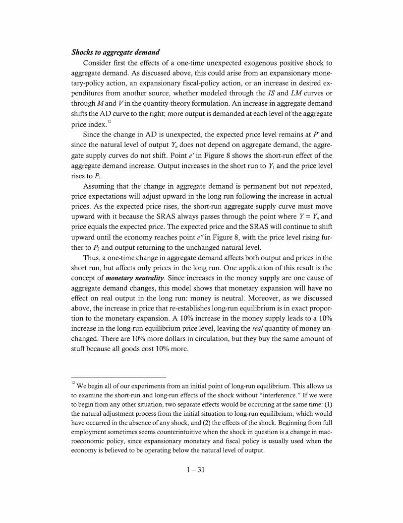
Shocks to aggregate demand Consider first the effects of a one-time unexpected exogenous positive shock to aggregate demand. As discussed above, this could arise from an expansionary mone-tary-policy action, an expansionary fiscal-policy action, or an increase in desired ex-penditures from another source, whether modeled through the IS and LM curves or through M and V in the quantity-theory formulation. An increase in aggregate demand shifts the AD curve to the right; more output is demanded at each level of the aggregate

price index.12

Since the change in AD is unexpected, the expected price level remains at Pe and since the natural level of output Yn does not depend on aggregate demand, the aggre-

gate supply curves do not shift. Point e′ in Figure 8 shows the short-run effect of the aggregate demand increase. Output increases in the short run to Y1 and the price level rises to P1. Assuming that the change in aggregate demand is permanent but not repeated, price expectations will adjust upward in the long run following the increase in actual prices. As the expected price rises, the short-run aggregate supply curve must move upward with it because the SRAS always passes through the point where Y = Yn and price equals the expected price. The expected price and the SRAS will continue to shift

upward until the economy reaches point e″ in Figure 8, with the price level rising fur-ther to P2 and output returning to the unchanged natural level. Thus, a one-time change in aggregate demand affects both output and prices in the short run, but affects only prices in the long run. One application of this result is the concept of monetary neutrality. Since increases in the money supply are one cause of aggregate demand changes, this model shows that monetary expansion will have no effect on real output in the long run: money is neutral. Moreover, as we discussed above, the increase in price that re-establishes long-run equilibrium is in exact propor-tion to the monetary expansion. A 10% increase in the money supply leads to a 10% increase in the long-run equilibrium price level, leaving the real quantity of money un-changed. There are 10% more dollars in circulation, but they buy the same amount of stuff because all goods cost 10% more.

12

We begin all of our experiments from an initial point of long-run equilibrium. This allows us to examine the short-run and long-run effects of the shock without “interference.” If we were to begin from any other situation, two separate effects would be occurring at the same time: (1) the natural adjustment process from the initial situation to long-run equilibrium, which would have occurred in the absence of any shock, and (2) the effects of the shock. Beginning from full employment sometimes seems counterintuitive when the shock in question is a change in mac-roeconomic policy, since expansionary monetary and fiscal policy is usually used when the economy is believed to be operating below the natural level of output.

1 – 32

P

Y

LRAS

Yn

SRAS’

Pe

AD

e

AD’

e’

Y1

P1

SRAS e’’ P2

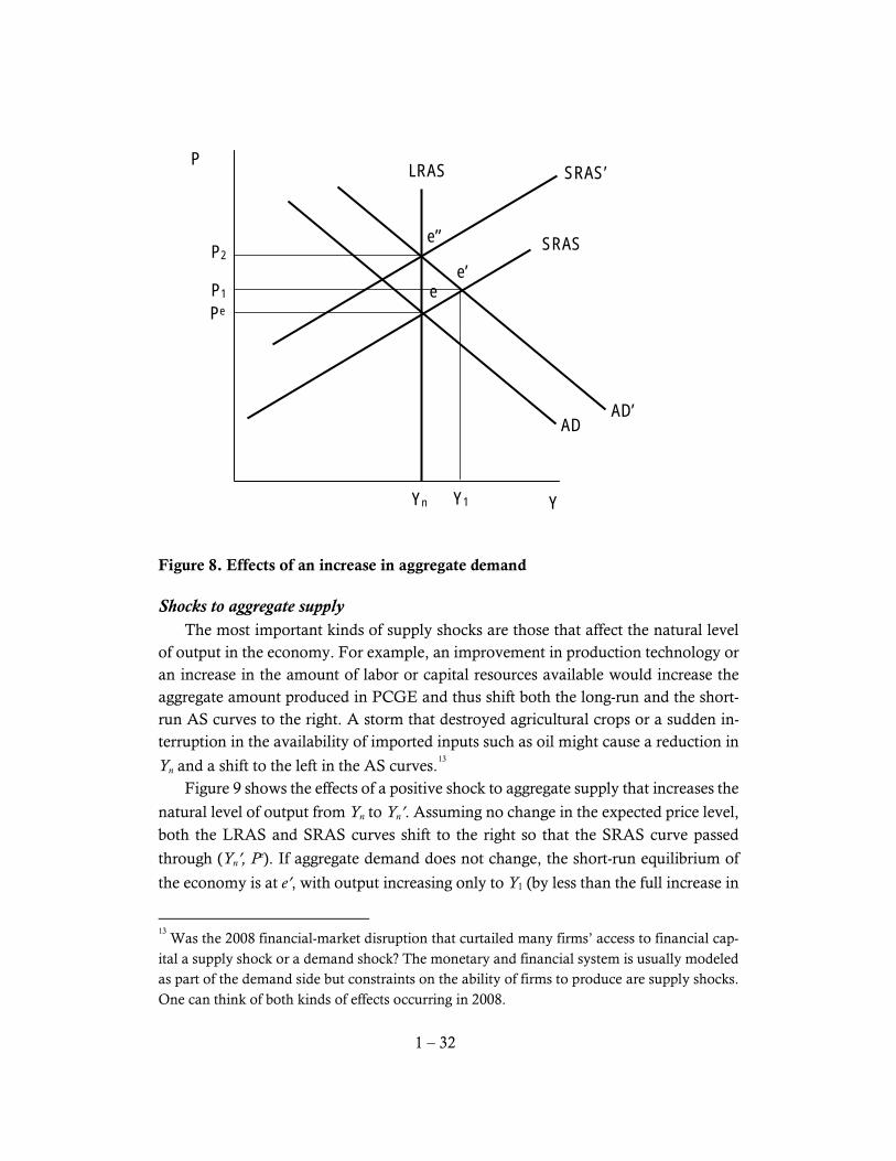
Figure 8. Effects of an increase in aggregate demand

Shocks to aggregate supply The most important kinds of supply shocks are those that affect the natural level of output in the economy. For example, an improvement in production technology or an increase in the amount of labor or capital resources available would increase the aggregate amount produced in PCGE and thus shift both the long-run and the short-run AS curves to the right. A storm that destroyed agricultural crops or a sudden in-terruption in the availability of imported inputs such as oil might cause a reduction in

Yn and a shift to the left in the AS curves.13

Figure 9 shows the effects of a positive shock to aggregate supply that increases the

natural level of output from Yn to Yn′. Assuming no change in the expected price level, both the LRAS and SRAS curves shift to the right so that the SRAS curve passed

through (Yn′, Pe). If aggregate demand does not change, the short-run equilibrium of

the economy is at e′, with output increasing only to Y1 (by less than the full increase in

13

Was the 2008 financial-market disruption that curtailed many firms’ access to financial cap-ital a supply shock or a demand shock? The monetary and financial system is usually modeled as part of the demand side but constraints on the ability of firms to produce are supply shocks. One can think of both kinds of effects occurring in 2008.

1 – 33

natural output) and price falling to P1. At e′ the economy is actually below its natural output, but it is unlikely that policymakers or the general public would easily recognize this gap because Yn is not directly observable and the absolute level of output has in-creased. In the long run, the expected price level will adjust downward following the de-

cline in prices. The eventual equilibrium of the economy will occur at e″, with price falling further to P2 and real output increasing to the new natural level. The one-time shocks depicted in Figure 8 and Figure 9 are interesting and they illustrate the short-run and long-run effects of demand and supply shocks. However, they are unrealistic in one important way: the economy in which they occur has neither ongoing growth in natural real output not inflation of the price level. Since output in nearly all modern economies is growing over time and inflation is a common phenomenon in most, we should also examine how the AS/AD model can be used to demonstrate the equilibrium evolution of such economies. We now turn to that task.

P

Y

LRAS

Yn

SRAS

Pe

AD

e

LRAS’

SRAS’

Yn’ Y1

P1

P2

e’ e’’

Figure 9. Effects of an aggregate supply shock

1 – 34

F. Dynamic Equilibrium in the AS/AD Model

As we examined in the first part of the course, modern economies grow; they do not stand still at a stationary point of equilibrium. If natural output and the determi-nants of aggregate demand (in particular, the money supply) are growing over time, then the economy does not remain perpetually in a static equilibrium such as the one depicted by point e in Figure 7. Instead, the whole system of AD and AS curves shifts over time, tracing out a dynamic time path of momentary equilibrium points. In this section, we first discuss why we would expect AS and AD curves to shift, then we examine the kind of equilibrium path that would results from steady growth in natural output and the money supply.

Why the AS curve shifts over time Recall that the natural level of output is the amount produced at full employment under perfect competition. With labor and capital resources fully employed, an in-crease in the amount of labor or capital available leads to a rise in natural output. Similarly an increase in the technological efficiency of production would result in greater natural output. Thus, in simple terms, we can think of Yn as reflecting the amount of output that can be produced by the available quantities of labor and capital using the best available technology. The labor force in most countries increases from year to year. Investment by firms in new capital typically exceeds the amount of old capital depreciating, so the amount of capital input also usually grows over time. Finally, technological progress means that economies are able to get more output from their resource inputs. Through growth in labor and capital inputs and technological progress, the natural level of output tends to grow steadily over time, pushing the aggregate supply curves to the right. On a steady-state growth path the annual percentage rate of growth in natural output would be constant, with the long-run aggregate-supply curve shifting to the right by a constant proportional amount each year.

Why the AD curve shifts over time The rightward shift in the aggregate demand curve over time is somewhat more complicated to explain than aggregate supply without resorting to formal, mathemat-ical analysis. To keep our initial exposition simple, we fall back on the simple quantity-theory model of aggregate demand that will suffice for most purposes. The simple AD curve of equation (2) shows an important mechanism by which aggregate demand moves in the long run: growth in the money supply. Most central banks accommodate growth in the economy’s transaction volume (i.e., growth in Y)

1 – 35

by expanding the supply of money. The growth in M pushes the AD curve up and to the right in proportion to the monetary expansion. You can see from equation (2) that if the central bank expands the money supply at the same rate that real output is growing (and if velocity is constant), then prices will be stable. The increases in M in the numerator and Y in the denominator will exactly balance with no change in V or P. If money growth exceeds real-output growth, then the quantity theory predicts that prices will rise to maintain the equation—there will be positive price inflation. If money growth falls short of output growth, then prices will tend to fall over time, which we call deflation.

Equilibrium with growth and inflation We have now established engines that can push the aggregate supply and aggregate demand curves to the right over time. Figure 10 shows a sequence of equilibria in an economy with both growth and inflation. Growth in labor, capital, and technological capability is increasing the natural level of output by 3 percent each year, from Yn,1 to Yn,2 to Yn,3 over the three years shown in Figure 10. This means that the LRAS curve is moving to the right as shown, by 3 percent per year. The money supply is growing at 5 percent per year, which shifts the aggregate demand curve upward and to the right by 5 percent each year. This is shown as AD1, AD2, and AD3 in Figure 10. (Of course, the AD curve should not be linear. It is drawn as a straight line in the figure for simplicity.) We assume that the behavior of the money supply and aggregate demand are cor-rectly predicted by everyone in the model—this is a smooth, ongoing process of growth and inflation with no shocks or surprises. Thus, price-setters and wage-setters would correctly anticipate that the price level would be P1 in the first period, P2 in the second period, and P3 in the third period. Since the SRAS curve always intersects the LRAS at the expected price level, it would move as shown by the SRAS1, SRAS2, and SRAS3 curves in Figure 10. Thus, the sequence of equilibrium will be traced out by the intersections of the AD and SRAS (and LRAS) curves at e1, e2, and e3. With AD shifting up 5 percent each year and AS shifting only 3 percent, the difference of 2 percent will be the increase in the price level. Thus, the economy pictured in Figure 10 would have a steady rate of infla-tion of 2 percent.

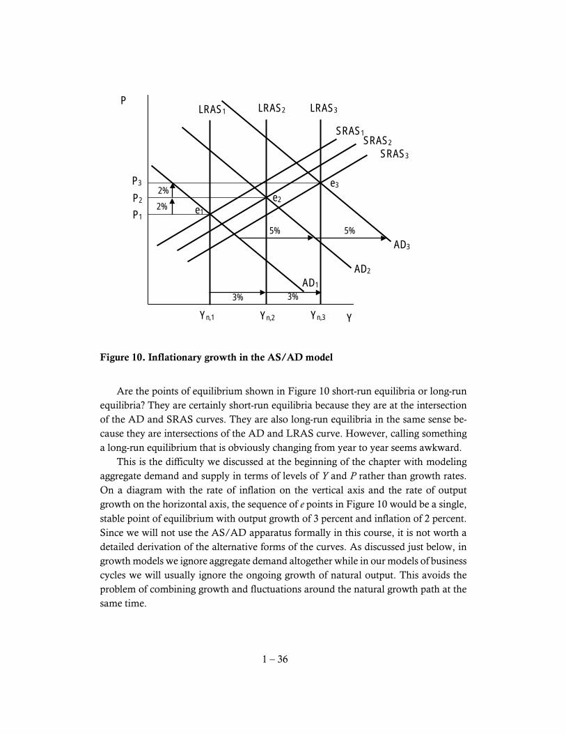
1 – 36

P

Y

LRAS2

Yn,2

SRAS2

P2

AD2

e2

Yn,1 Yn,3

LRAS1 LRAS3

AD1

AD3

e3

e1

SRAS3

SRAS1

P1

P3

3% 3%

5% 5%

2% 2%

Figure 10. Inflationary growth in the AS/AD model

Are the points of equilibrium shown in Figure 10 short-run equilibria or long-run equilibria? They are certainly short-run equilibria because they are at the intersection of the AD and SRAS curves. They are also long-run equilibria in the same sense be-cause they are intersections of the AD and LRAS curve. However, calling something a long-run equilibrium that is obviously changing from year to year seems awkward. This is the difficulty we discussed at the beginning of the chapter with modeling aggregate demand and supply in terms of levels of Y and P rather than growth rates. On a diagram with the rate of inflation on the vertical axis and the rate of output growth on the horizontal axis, the sequence of e points in Figure 10 would be a single, stable point of equilibrium with output growth of 3 percent and inflation of 2 percent. Since we will not use the AS/AD apparatus formally in this course, it is not worth a detailed derivation of the alternative forms of the curves. As discussed just below, in growth models we ignore aggregate demand altogether while in our models of business cycles we will usually ignore the ongoing growth of natural output. This avoids the problem of combining growth and fluctuations around the natural growth path at the same time.

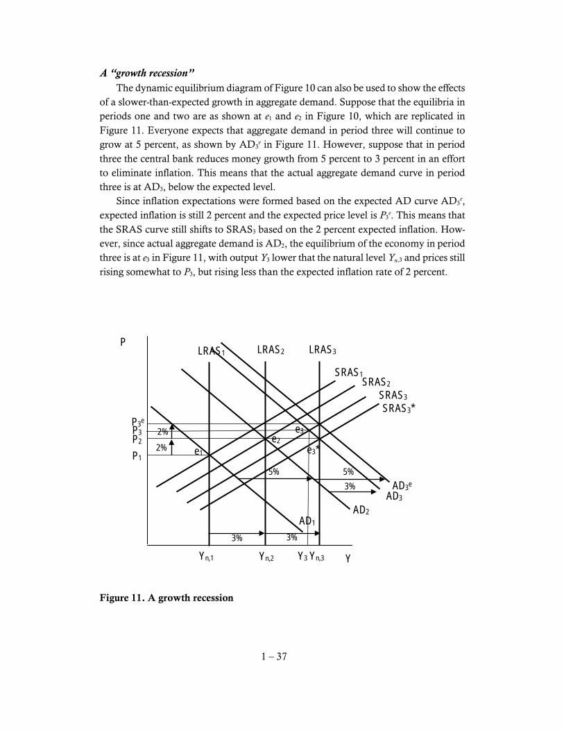
1 – 37

A “growth recession” The dynamic equilibrium diagram of Figure 10 can also be used to show the effects of a slower-than-expected growth in aggregate demand. Suppose that the equilibria in periods one and two are as shown at e1 and e2 in Figure 10, which are replicated in Figure 11. Everyone expects that aggregate demand in period three will continue to grow at 5 percent, as shown by AD3

e in Figure 11. However, suppose that in period three the central bank reduces money growth from 5 percent to 3 percent in an effort to eliminate inflation. This means that the actual aggregate demand curve in period three is at AD3, below the expected level. Since inflation expectations were formed based on the expected AD curve AD3

e, expected inflation is still 2 percent and the expected price level is P3

e. This means that the SRAS curve still shifts to SRAS3 based on the 2 percent expected inflation. How-ever, since actual aggregate demand is AD2, the equilibrium of the economy in period three is at e3 in Figure 11, with output Y3 lower that the natural level Yn,3 and prices still rising somewhat to P3, but rising less than the expected inflation rate of 2 percent.

P

Y

LRAS2

Yn,2

SRAS2

P2

AD2

e2

Yn,1 Yn,3

LRAS1 LRAS3

AD1

AD3e

e3

e1

SRAS3

SRAS1

P1

P3e

3% 3%

5% 5%

2% 2%

AD3

Y3

P3

3%

SRAS3*

e3*

Figure 11. A growth recession

1 – 38

This situation is sometimes called a “growth recession.” It does not officially qual-ify as a recession because real output continues to grow. However, the growth rate of output in period three is less than the growth in natural output—real output falls below its growth trend—hence the term growth recession. The situation shown in Figure 11 suggests that reducing the rate of inflation can be costly—it induces a temporary reduction in output growth. This change is tempo-rary because once expectations adjust to the change in monetary growth, the SRAS curve will adjust downward to reflect lowered inflation expectations and output will return to its natural growth path. Depending on the size of the gap between Y3 and Yn,3 and the length of time required for expectations adjustment to occur, this cost of dis-

inflation could be small or large.14

It is worth noting what would have happened if everyone had correctly anticipated the reduction in money growth in time to set wages and prices. In Figure 11, the ex-pected price level for period three would have remained at P2 rather than rising to P3

e, which would have shifted the SRAS curve further to the right to SRAS3*. In that case, equilibrium in period three would be at e3*, with output growing at the natural growth rate and inflation immediately jumping to the 0 percent rate that is consistent with the lowered rate of money growth. This makes it clear that it is the delayed adjustment of wages and prices based on faulty inflation expectations that causes the growth recession in Figure 11. In the sim-ple AS/AD model, a fully credible disinflation that is known about far enough in ad-vance to allow wage and price setters to adjust will not lead to a reduction of output below its natural level. Disinflation can be costly, but in this model it need not be if monetary policy has sufficient credibility.

G. A Preview of Romer’s Text from the Perspective of Aggregate Supply/Demand

Growth models Chapters 1 through 3 of Romer’s textbook describe the evolution of economic growth theory from the Solow model of the 1950s through the optimal growth models that Cass and Koopmans built on Ramsey’s framework in the 1960s to the endogenous

14

In a famous article, Laurence Ball (1994) has estimated the “sacrifice ratio”—the amount of forgone output for each percentage-point reduction in inflation—for late 20th century disinfla-tions.

1 – 39

growth models of Paul Romer and others since the 1980s. These growth models all describe the evolution over time in the natural level of output, ignoring any role of aggregate demand. The emphasis in these models is on increases in aggregate supplies of labor and capital resources and on technological progress—i.e., on the supply side of the macro-economy. By focusing exclusively on aggregate supply, these models ignore any de-mand-related fluctuations of output relative to its long-run equilibrium growth path, such as those in Figure 11.

Real business cycles Romer’s Chapter 5 presents a stylized version of the real business cycle (RBC) model. This model is also entirely based on the supply side of the economy, but rather than looking exclusively at smooth trend movements in natural output it considers situations where the increase in natural output is subject to shocks. These supply shocks, which can be bursts of rapid or slow technological progress, cause the amount of rightward shift in the natural level of output and the LRAS curve to vary from year to year. Like the growth models, the real business cycle model has no role for aggregate demand. It explains business cycles as fluctuations in supply-driven growth of Yn, not as movements of Y around a smoothly growing Yn. This difference is of critical im-portance for macroeconomic policy. Since Yn is the level of output generated by the PCGE model, an appropriate goal of macro policy is to keep Y close to Yn. If business cycles are fluctuations of Y around Yn, then countercyclical policy to diminish these movements is desirable. If, as in the RBC model, it is the natural level of output itself that fluctuates, then the resulting cyclical movements in output are both “natural” and desirable. It would be inappropriate for monetary and fiscal policies to attempt to smooth them out. (And of course the RBC model predicts that monetary and fiscal policy, because they affect AD, would not affect output anyway.)

The IS/LM model Romer introduces the IS/LM framework and a variant—the IS/MP model—in Chapter 6. The IS/LM model was developed for a closed economy—one with no trade or credit transactions with the rest of the world. The IS/LM and IS/MP models are models of aggregate demand. To the extent that they pretend, on their own, to be theories of real output determination, they are making the implicit assumption of fixed prices—a horizontal aggregate supply curve. This assumption is probably not very realistic even in the short run and is clearly inap-propriate in the long run. A more appropriate characterization of the macroeconomy would use these models to explain the AD curve, then combine them with theories of aggregate supply.

1 – 40

H. Suggestions for Further Reading

Much of the material discussed in this chapter is covered in standard introductory or intermediate macroeconomics texts. One of the best at each level is written by N. Gregory Mankiw: his Macroeconomics is an intermediate text and his Introduction to Macroeconomics is more basic. Other standard intermediate texts are those of Olivier Blanchard; Robert Hall and John Taylor; and Andrew Abel and Ben Bernanke. (All of these intermediate texts are called Macroeconomics.) Another useful intermediate text is Macroeconomics: A European Text by Michael Burda and Charles Wyplosz. This text is often used in Econ 304 at Reed; it contains a more complete treatment of open-economy and international issues than the American texts.

I. Works Cited in Text

Ball, Laurence. 1994. What Determines the Sacrifice Ratio? In Monetary Policy, edited by N. G. Mankiw. Chicago and London: University of Chicago Press.

Fisher, Irving. 1913. The Purchasing Power of Money: Its Determination and Relation to Credit, Interest and Crises. New York: Macmillan.

Hicks, John R. 1937. Mr. Keynes and the 'Classics'. Econometrica 5 (2):147-159. Leijonhufvud, Axel. 1968. On Keynesian Economics and the Economics of Keynes: A Study

in Monetary Theory. New York: Oxford University Press. Parker, Jonathan A. 2011. On Measuring the Effects of Fiscal Policy in Recessions.

Journal of Economic Literature 49 (3):703-718. Pigou, A. C. 1933. The Theory of Unemployment. London: Macmillan. Ramey, Valerie A. 2011. Can Government Purchases Stimulate the Economy? Journal

of Economic Literature 49 (3):673-685. Taylor, John B. 2011. An Empirical Analysis of the Revival of Fiscal Activism in the

2000s. Journal of Economic Literature 49 (3):686-702.