8. turbulence modelling in cfd spring 2007 · cfd 8-1 david apsley 8. turbulence modelling in cfd...
TRANSCRIPT
CFD 8-1 David Apsley
8. TURBULENCE MODELLING IN CFD SPRING 2007 8.1 Turbulence models for general-purpose CFD 8.2 Linear eddy-viscosity models 8.3 Non-linear eddy-viscosity models 8.4 Differential stress models 8.5 Implementation of turbulence models in CFD 8.1 Turbulence Models For General-Purpose CFD Turbulence models for general-purpose CFD must be frame-invariant – i.e. independent of any particular coordinate system – and hence must be expressed in tensor form. This rules out simpler models of boundary-layer type (e.g. mixing-length models). Turbulent flows are computed either by solving the Reynolds-averaged Navier-Stokes equations with suitable models for turbulent fluxes or by computing the fluctuating quantities directly. The main approaches are summarised below. Reynolds-Averaged Navier-Stokes (RANS) Models • Linear eddy-viscosity models (EVM) – assume that the (deviatoric) turbulent stress is proportional to the mean strain; – use an eddy viscosity constructed from turbulence scalars (usually k + one other),
determined by solving transport equations. • Non-linear eddy-viscosity models (NLEVM) – assume that the turbulent stress is a non-linear function of mean strain and vorticity; – use coefficients constructed from turbulence scalars (usually k + one other),
determined by solving transport equations; – mimic response of turbulence to certain important types of strain. • Differential stress models (DSM) – aka Reynolds-stress transport models (RSTM) or second-order closure (SOC); – solve transport equations for all turbulent fluxes. Computation of fluctuating quantities • Large-eddy simulation (LES) – compute time-varying flow, but model sub-grid-scale motions. • Direct numerical simulation (DNS) – no modelling; resolve the smallest scales of the flow.

CFD 8-2 David Apsley
8.2 Linear Eddy-Viscosity Models 8.2.1 General Form Stress-strain constitutive relation:
iji
j
j
itji k
x
U
x
Uuu
��3
2�� −��
�
�
��
�
�
∂∂
+∂∂
=− , tt ���� = (1)
The eddy viscosity � t is derived from turbulent quantities such as the turbulent kinetic energy k and dissipation rate � . These quantities are themselves determined by solving scalar-transport equations (see below). A typical shear stress and normal stress are given by
���
����
�
∂∂+
∂∂=−
x
V
y
Uuv t
��
kx
Uu t �3
22� 2 −∂∂=−
From these the other stress components are easily deduced by inspection/cyclic permutation. General Comments • � is a physical property of the fluid and can be measured; � t is a hypothetical property
of the flow and must be modelled. • �
t varies with position. • At high Reynolds numbers, � t � � throughout much of the flow. Advantages • Easy to implement in viscous solvers. • Extra viscosity aids stability. • Some theoretical foundation in simple shear flows. Disadvantages • Little turbulence physics; in particular, anisotropy and history effects are neglected. • Turbulent transport of momentum is determined by a single scalar � t, so at most one
Reynolds stress ( uv− ) can be represented accurately; such models are questionable in complex flow.
Most eddy-viscosity models in general-purpose CFD codes are of the 2-equation type; (i.e. scalar-transport equations are solved for 2 turbulent scales). The commonest types are k-� and k-� models, for which specifications are given below.
CFD 8-3 David Apsley
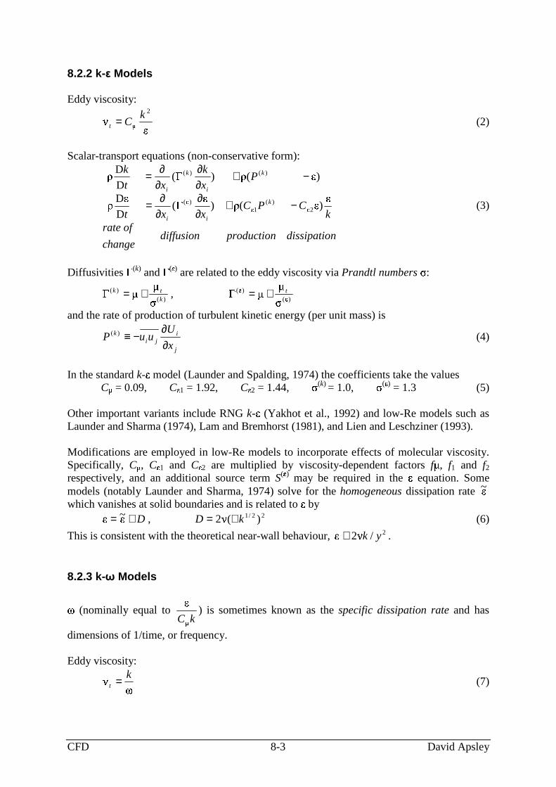
8.2.2 k- Models Eddy viscosity:
��
2� kCt = (2)
Scalar-transport equations (non-conservative form):
ndissipatioproductiondiffusionchange
ofratek
CPCxxt
Px
k
xt
k
k
ii
k
i
k
i �)
�(�)
��(
D
�D�
)�
(�)�
(D
D�
2�)(1�)�(
)()(
−+∂∂
∂∂=
−+∂∂
∂∂=
(3)
Diffusivities � (k) and � (� ) are related to the eddy viscosity via Prandtl numbers � :
)�(
)�()(
)( �, � t
ktk +=+=
and the rate of production of turbulent kinetic energy (per unit mass) is
j
iji
k
x
UuuP
∂∂
−≡)( (4)
In the standard k-� model (Launder and Spalding, 1974) the coefficients take the values C � = 0.09, C 1 = 1.92, C 2 = 1.44, � (k) = 1.0, � ( ) = 1.3 (5) Other important variants include RNG k-� (Yakhot et al., 1992) and low-Re models such as Launder and Sharma (1974), Lam and Bremhorst (1981), and Lien and Leschziner (1993). Modifications are employed in low-Re models to incorporate effects of molecular viscosity. Specifically, C � , C 1 and C 2 are multiplied by viscosity-dependent factors f� , f1 and f2 respectively, and an additional source term S( ) may be required in the � equation. Some models (notably Launder and Sharma, 1974) solve for the homogeneous dissipation rate �~ which vanishes at solid boundaries and is related to � by 22/1 )(�2,�~� kDD ∇=+= (6)
This is consistent with the theoretical near-wall behaviour, 2/�2� yk∼ . 8.2.3 k- Models
� (nominally equal to kC �
�) is sometimes known as the specific dissipation rate and has
dimensions of 1/time, or frequency. Eddy viscosity:
�� kt = (7)

CFD 8-4 David Apsley
Scalar-transport equations:
)����
�(�)
��(
D
�D�
)��
(�)�
(D
D�
2)()�(
)()( *
−+∂∂
∂∂=
−+∂∂
∂∂=
k
tii
k
i
k
i
Pxxt
kPx
k
xt
k
(8)
The diffusivities of k and � are related to the eddy-viscosity:
)�()�(
)()( �
, � tktk +=+=
The original k-� model was that of Wilcox (1988a) with coefficients taking the values
100
9� * = , 9
5� = , 40
3�= , � (k) = 2.0, � ( � ) = 2.0 (9)
The model was further developed by Wilcox (1998) in his book, with the coefficients becoming functions of the turbulent Reynolds number. Menter (1994) devised a shear-stress-transport (SST) model. The model, which is expressed in k-� form, blends the k-� model (which is – allegedly – superior in the near-wall region), with the k-� model (which is less sensitive to the level of turbulence in the free stream). All models of k-� type suffer from a problematic wall boundary condition (� � as y → 0). 8.2.4 Behaviour of Linear Eddy-Viscosity Models in Simple Shear In simple shear flow the shear stress is
y
Uuv t ∂
∂=− ��
The three normal stresses are predicted to be equal:
kwvu3
2222 ===
whereas, in practice, there is considerable anisotropy; e.g. in the log-law region:
6.0:4.0:0.1:: 222 ≈wvu Actually, in simple shear flows, this is not a problem, since only the gradient of the shear
stress uv� plays a dynamically-significant role in the mean-momentum equation. However, it is a warning of more serious problems in complex flows.
uv
U(y)
y

CFD 8-5 David Apsley
8.3 Non-Linear Eddy-Viscosity Models 8.3.1 General Form The stress-strain relationship for linear eddy-viscosity models gives for the deviatoric Reynolds stress (i.e. subtracting the trace):
��
�
�
��
�
�
∂∂
+∂∂
=−i
j
j
itijji x
U
x
Ukuu ��
3
2
Dividing by k and writing �/� 2� kCt = gives
��
�
�
��
�
�
∂∂
+∂∂
−=−i
j
j
iij
ji
x
U
x
UkC
k
uu ��3
2 � (10)
We define the LHS of (10) as the anisotropy tensor aij; it is the dimensionless and traceless form of the Reynolds stress:
ijji
ij k
uua �
3
2−≡ (11)
For the RHS of (10), the symmetric and antisymmetric parts of the mean-velocity gradient are called the mean strain and mean vorticity tensors, respectively:
)(2
1�,)(
2
1
i
j
j
iij
i
j
j
iij x
U
x
U
x
U
x
US
∂∂
−∂∂
≡∂
∂+
∂∂
≡ (12)
These can be made non-dimensional using the turbulent timescale k/� . Using lower case for the non-dimensional forms:
ijijijij
kS
ks
��,� ≡≡ (13)
Equation (10) can then be written in the simpler form ijij sCa 2−=
or, sa 2C−= (14)
Hence, the constitutive relation for linear eddy-viscosity models simply says: “anisotropy tensor is proportional to dimensionless mean strain”
The main idea of non-linear eddy-viscosity models is to generalise this to a non-linear relationship between the anisotropy tensor and the mean strain and vorticity: ),(2 sNLsa +−= C (15)
Additional non-linear components cannot be completely arbitrary, but must be symmetric and traceless. For example a quadratic NLEVM must be of the form
)}{(
�)(
�)}{(
� 22
312
322
312
1
�IssIss
sa
−+−+−+
−= C (16)
where { .} denotes a trace and I is the identity matrix: iiMtrace ≡≡ )(}{ MM , ijij )( ≡I (17)
We shall see below that an appropriate choice of the coefficients �
1, �
2 and �
3 allows the model to reproduce the correct anisotropy in simple shear. Theory (based on the Cayley-Hamilton Theorem) shows that the most general relationship

CFD 8-6 David Apsley
involves ten independent tensor bases and includes terms up to the 5th power in s and :
),(10
1�
�� sTa �=
= C (18)
where all T � are linearly-independent, symmetric, traceless, second-rank tensor products of s and . One possible choice of bases (but by no means the only one) is Linear: sT =1
Quadratic: IssT }{ 2312
2 −=
ssT −=3
I��T }{ 2312
4 −=
Cubic: IssssT }{}{ 32222
5 −−+=
ssT 226 −=
Quartic: IsIssssT }{)}{} ({ 22322
31222222
7 −−−+=
)} ({ 22122
8 sssssssT −−−=
)} ({ 22122
9 ssssT −−−=
Quintic: ssT 222210 −=
Exercise. (i) Prove that all these bases are symmetric and traceless. (ii) Show that bases T5 – T10 vanish in 2-d incompressible flow. The first base corresponds to a linear eddy-viscosity model and the next three to the quadratic extension in equation (16). T5, T7, T8, T9 contain multiples of earlier bases and hence could be replaced by simpler forms; however, the bases chosen here ensure that they vanish in 2-d incompressible flow. A number of routes have been taken in devising such NLEVMs, including: • assuming the form of the series expansion to quadratic or cubic order and simply
calibrating against important flows (e.g. Speziale, 1987; Craft, Launder and Suga, 1996);
• simplifying a differential stress model by an explicit solution (e.g. Speziale and Gatski, 1993) or by successive approximation (e.g. Apsley and Leschziner, 1998);
• renormalisation group methods (e.g. Rubinstein and Barton, 1990); • direct interaction approximation (e.g Yoshizawa, 1987). In devising such NLEVMs, model developers have sought to incorporate such physically-significant properties as realisability:
)inequalitySchwartzCauchy(1
stresses) normal positive(0
2�
2�
2��
2�
−≤
≥
uu
uu
u
(19)

CFD 8-7 David Apsley
8.3.2 Cubic Eddy-Viscosity Models The preferred level of modelling at the University of Manchester is a cubic eddy viscosity model, which can be written in the form
)(�)}{}{(�}{�}{�)}{(
�)(
�)}{(
�222
432222
32
22
1
2312
322
312
1
��
ssIsssssss
IssIss
sa
−−−−+−−−−+−+−+
−= fC
(20) Note the following properties (some of which will be developed further below and on the example sheet). (i) A cubic stress-strain relationship is the minimum order with at least the same number
of independent coefficients as the anisotropy tensor (i.e. 5). In this case it will be precisely 5 if we assume
�3 = 0 (see (vi) below) and note that the �
1 and �2 terms are
tensorially similar to the linear term (see (iv) below). (ii) The first term on the RHS corresponds to a linear eddy-viscosity model. (iii) The various non-linear terms evoke sensitivities to specific types of strain: – the quadratic (
�1,
�2,
�3) terms evoke sensitivity to anisotropy;
– the cubic �1 and �
2 terms evoke sensitivity to curvature; – the cubic �
4 term evokes sensitivity to swirl. (iv) The �
1 and �2 terms are tensorially proportional to the linear term; however they (or
rather their difference) provide a sensitivity to curvature, so have been kept distinct. (v) The �
3 and �4 terms vanish in 2-d incompressible flow.
(vi) Theory and experiment indicate that pure rotation generates no turbulence. This implies that
�3 ought to be 0, at least in the limit 0→S .
As an example of such a model we cite the Craft et al. (1996) model in which coefficients are functions of the mean-strain invariants and turbulent Reynolds number:
�~�,])400
()90
(exp[1
�35.01
)]36.0exp(1[3.0
222/1�
2/3
�75.0�k
RRR
f
eC
ttt =−−−=
+−−=
(21)
where
)�
,max(�~�,��
2�
,2 Sk
SSS ijijijij === (22)
The coefficients of the non-linear terms are (in the present notation): ��321 )04.1,4.0,4.0()
�,
�,
�( fC−−=
�3�4321 )80,0,40,40()�,�,�,�( fC−= (23)
Non-linearity is built into both tensor products and strain-dependent coefficients – notably C � . The model is completed by transport equations for k and �~ . Mean strain and vorticity are non-dimensionalised using �~ rather than � .
CFD 8-8 David Apsley
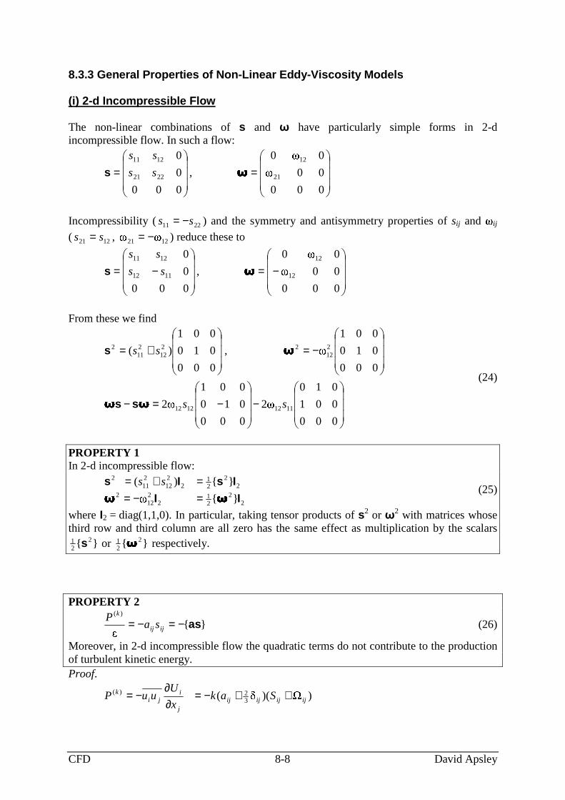
8.3.3 General Properties of Non-Linear Eddy-Viscosity Models (i) 2-d Incompressible Flow The non-linear combinations of s and have particularly simple forms in 2-d incompressible flow. In such a flow:
���
�
�
���
�
�
=���
�
�
���
�
�
=000
00�
0�0
,
000
0
0
21
12
2221
1211�ss
ss
s
Incompressibility ( 2211 ss −= ) and the symmetry and antisymmetry properties of sij and �
ij
( 1221 ss = , 1221�� −= ) reduce these to
���
�
�
���
�
�
−=���
�
�
���
�
�
−=000
00�
0�0
,
000
0
0
12
12
1112
1211�ss
ss
s
From these we find
���
�
�
���
�
�
−���
�
�
���
�
�
−=−
���
�
�
���
�
�
−=���
�
�
���
�
�
+=
000
001
010�2
000
010
001�2
000
010
001�,
000
010
001
)(
11121212
212
2212
211
2
ss
ss
��
�
ss
s
(24)
PROPERTY 1 In 2-d incompressible flow:
2
221
2212
22
221
2212
211
2
}{�
}{)(
II
IsIs�� =−=
=+= ss (25)
where I2 = diag(1,1,0). In particular, taking tensor products of s2 or 2 with matrices whose third row and third column are all zero has the same effect as multiplication by the scalars
}{ 221 s or }{ 2
21 � respectively.
PROPERTY 2
}{�
)(
as−=−= ijij
k
saP
(26)
Moreover, in 2-d incompressible flow the quadratic terms do not contribute to the production of turbulent kinetic energy. Proof.
)
)(
( 32)(
ijijijijj
iji
k Sakx
UuuP ++−=
∂∂
−=

CFD 8-9 David Apsley
Now 0�
)�
( 32 =+ ijijija since
ij is antisymmetric, whilst incompressibility implies
0�
== iiijij SS . Hence,
ijijk SkaP −=)(
or
}{�
)(
as−=−= ijij
k
saP
This is true for any incompressible flow, but, in the 2-d case, multiplying (20) by s, taking the trace and using the results (25) it is found that the contribution of the quadratic terms to { as} is 0. PROPERTY 3 In 2-d incompressible flow the � 3- and � 4-related terms of the non-linear expansion (20) vanish. Proof. Substitute the results (25) for s2 and 2 into (20). (ii) Particular Types of Strain The non-linear constitutive relationship (20) allows the model to mimic the response of turbulence to particular important types of strain. PROPERTY 4 The quadratic terms yield turbulence anisotropy in simple shear:
6
�)
��(
3
2
12
�)
��6
�(
3
2
12
�)
��6
�(
3
2
2
31
2
2
321
2
2
321
2
−−=
−−+=
−++=
k
w
k
v
k
u
where y
Uk
∂∂= �� (27)
This may be deduced by substituting the results (24) into (20), noting that s11 = 0, whilst
�2
1�2
1�1212 =
∂∂==
y
Uks
As an example the figure right shows application of the Apsley and Leschziner (1998) model to computing the Reynolds stresses in channel flow.
0
50
100
150
200
250
300
350
400
450
0 1 2 3 4 5 6 7 8
y+
uu+vv+ww+-uv+

CFD 8-10 David Apsley
PROPERTY 5 The � 1 and � 2-related cubic terms yield the correct sensitivity to curvature.
In curved shear flow, c
ss
R
U
x
V
R
U
y
U −=∂∂
∂∂
=∂∂
, , where Rc is radius of curvature. From (24),
)�(2}{}{ 212
212
22 −≡+ ss where
���
����
�+
∂∂
=���
����
�−
∂∂
=c
ss
c
ss
R
U
R
U
R
U
R
Us
2
1�,2
11212
Hence,
c
ss
R
U
R
Uk
∂∂
−≡+ 222 )�(2}{}{s
Inspection of the production terms in the stress-transport equations (Section 7.4) shows that curvature is stabilising (reducing turbulence) if Us increases in the direction away from the centre of curvature (∂Us/∂R > 0) and destabilising (increasing turbulence) if Us decreases in the direction away from the centre of curvature (∂Us/∂R < 0). In the constitutive relation (20) the response is correct if � 1 and � 2 are both positive. PROPERTY 6 In 3-d flows, the � 4-related term evokes the correct sensitivity to swirl.
'stable' curvature(reducing turbulence)
'unstable' curvature(increasing turbulence)
UW

CFD 8-11 David Apsley
8.4 Differential Stress Modelling Differential stress models (aka Reynolds-stress transport models or second-order closure)
solve a separate scalar-transport equation for each stress component jiuu :
)��
(�
D
)(D�ijijijij
k
ijkji FPx
d
t
uu−+++
∂∂
= (28)
(For a derivation see the course notes for the “Boundary Layers” module). Such models, in principle, contain much more turbulence physics because the rate-of-change, advection and production terms are exact. The nearest thing to a standard model is a high-Re closure based on that of Launder et al. (1975) and Gibson and Launder (1978). Term Name and role Model
t
uu ji
D
)(D� RATE OF CHANGE (time derivative + advection) Transport with the mean flow.
EXACT
ijP PRODUCTION (mean strain) Generation of turbulence energy from the mean flow.
EXACT
k
ikj
k
jkiij x
Uuu
x
UuuP
∂∂
−∂∂
−≡
Fij
PRODUCTION (body forces) Generation of turbulence energy by body forces.
EXACT (in principle)
ijjiij ufufF +≡
ijkd DIFFUSION Spatial redistribution.
)()�
�� �
( jil
lksklijk uu
x
uukCd
∂∂+=
ijΦ PRESSURE-STRAIN Redistribution of turbulence energy between components.
)()2()1( ���� wijijijij ++=
)�
(�
�
32
1)1(
ijjiij kuuk
C −−=
)�
(�
31
2)2(
ijkkijij PPC −−=
nij
wji
wij
kijkkjikijlkklw
ij
y
kCfCuu
kC
fnnnnnn
�
�/
,�
�� ~
)� ~� ~�� ~
(�
2/34/3�)2()(
2)(
1
23
23)(
=+=
−−=
ijε DISSIPATION Removal of turbulence energy by viscosity
ijij� ��
32=
Typical values of the constants are: 3.0,5.0,6.0,8.1 )(
2)(
121 ==== ww CCCC (29)

CFD 8-12 David Apsley
Energy in Turbulent Fluctuations In simple shear flow (where ∂U/∂y is the only non-zero mean-velocity gradient) the production terms of the normal stresses are:
0,2 332211 ==∂∂−= PP
y
UuvP
Hence, production of turbulence energy predominantly feeds the 2u component. Energy is then transferred to fluctuations in the cross-stream directions by the redistributive effect of pressure fluctuations. At small scales local gradients are sufficiently large for viscosity to dissipate turbulent energy. There is a continual energy cascade from the energy entering the turbulence at the large scales of the flow, though shear instabilities continually producing eddies at smaller scales, until ultimately energy is removed by viscosity.
PRODUCTION ADVECTION by mean flow
2u 2v2w
REDISTRIBUTION
DISSIPATION by viscosity
by pressure fluctuations

CFD 8-13 David Apsley
The stress-transport equations must be supplemented by a means of specifying � – typically
by its own transport equation, or one for a related quantity such as � . As is suggested by the table, the most significant term requiring modelling is the pressure-strain correlation (which is formed, in practice, by the average product of pressure fluctuations and fluctuating velocity gradients). This term is traceless (i.e. the sum of the diagonal terms 0
���
332211 =++ ) and its accepted role is to promote isotropy – hence the
form of model for )1(�
ij and )2(�
ij . Near walls this isotropising tendency must be over-ridden,
necessitating a “wall-correction” term )(� wij .
Where body forces are present (e.g. in buoyant or rotating flows) additional production terms must be included. General Assessment of DSMs For: • Include more turbulence physics than eddy-viscosity models. • Advection and production terms (“energy-in” terms) are exact and do not need
modelling. Against: • Models are very complex and many important terms (particularly the redistribution
and dissipation terms) require modelling. • Models are very expensive computationally (6 stress-transport equations in 3
dimensions) and tend to be numerically unstable (only the small molecular viscosity contributes to any sort of gradient diffusion term).
Other DSMs of Interest • Speziale et al. (1991) – non-linear
�ij formulation, eliminating wall-correction terms;
• Craft (1998) – low-Re DSM, attempting to eliminate wall-dependent parameters; • Jakirli � and Hanjali � (1995) – low-Re DSM admitting anisotropic dissipation; • Wilcox (1988b) – low-Re DSM, with � rather than
� as additional turbulent scalar.
Excellent references for developments in Reynolds-stress transport modelling can be found in Launder (1989) and Hanjali � (1994).

CFD 8-14 David Apsley
8.5 Implementation of Turbulence Models in CFD 8.5.1 Transport Equations The implementation of a turbulence model in CFD requires:
(1) a means of specifying the turbulent stresses jiuu , by either:
– a constitutive relation (eddy-viscosity models), or – individual transport equations (differential stress models); (2) the solution of additional scalar-transport equations. Special Considerations for the Mean Flow Equations
• jiuu� represents a turbulent flux of Ui-momentum in the xj direction, but only a part
of this can be treated implicitly as a diffusion-like term. e.g. for the U equation through a face normal to the y direction:
���� ����� �����
sourcetodtransferrepart
diffusive
t termslinearnonx
V
y
Uuv )()(�� −+
∂∂+
∂∂=−
The non-diffusive part of the flux is transferred to the source term (and treated explicitly – i.e. held constant for that iteration). Nevertheless, it is still treated in a conservative fashion; i.e. it is worked out on a cell face so that the mean momentum lost by one cell is equal to that gained by its neighbour.
• The lack of a turbulent viscosity in differential stress models can lead to numerical
instability. This can be addressed by the use of “effective viscosities” – see below. Special Considerations for the Turbulence Equations • They are usually source-dominated; i.e. the most significant terms are production,
redistribution and dissipation; (this is sometimes used as an excuse for a low-order advection scheme).
• Variables such as k and
� must be non-negative. This demands:
– care in discretising the source term (see below); – use of an unconditionally-bounded advection scheme. Source-Term Linearisation For Non-Negative Quantities The general discretised scalar-transport equation for a control volume centred on node P is PPP
FFFPP sbaa φ+=φ−φ �
For stability one requires 0≤Ps
To ensure non-negative φ one requires, in addition,

CFD 8-15 David Apsley
0≥Pb You should, by inspection of the k and
� transport equations (3), be able to identify how the
source term is linearised in this way, with one positive part and one negative part, the latter preferably proportional to the transported variable, k or
�.
If bP < 0 for a quantity such as k or
� which is always non-negative (e.g. due to transfer of
non-linear parts of the advection term or non-diffusive fluxes to the source term) then, to ensure that the variable doesn’ t become negative, the source term should be rearranged as
0
)(*
→
φφ
+→
P
P
P
PPP
b
bss
(30)
where * denotes the current value of a variable. 8.5.2 Wall Boundary Conditions At walls the no-slip boundary condition applies, so that both mean and fluctuating velocities vanish. At high Reynolds numbers this presents three problems: • there are very large flow gradients; • wall-normal fluctuations are suppressed (i.e. selectively damped); • viscous and turbulent stresses are of comparable magnitude. There are two main ways of handling this in turbulent flow: •••• low-Reynolds-number turbulence models – resolve the flow right up to the wall with a very fine grid and viscous
modifications to the turbulence equations to ensure the correct near-wall rather than log-layer behaviour;
•••• wall functions – use a coarser grid and assume theoretical profiles between the near-wall
node and the boundary. Low-Reynolds-Number Turbulence Models • Aim to resolve the flow right up to the boundary. • Have to include effects of molecular viscosity in the coefficients of the eddy-viscosity
formula and � (or � ) transport equations.
• Try to ensure the theoretical near-wall behaviour:
)0(�,constant~�2
~�, 32
2 →∝∝ yyy
kyk t (31)
• Full resolution of the flow requires the near-wall node to satisfy y+ ≤ 1, where
�
� yuy ≡+ , �/�
� wu = (32)
This can be very computationally demanding, particularly for high-speed flows.

CFD 8-16 David Apsley
High-Reynolds-Number Turbulence Models • Bridge the near-wall region with wall
functions; i.e. assume profiles (based on boundary-layer theory) between near-wall node and boundary.
• OK if near equilibrium (e.g. slowly-developing
boundary layers), but dodgy in highly non-equilibrium regions (particularly near impingement, separation or reattachment points).
• The near-wall node should ideally be placed in the region 30 < y+ < 50 (range 15 -150
generally acceptable). This means that numerical meshes cannot be arbitrarily refined close to solid boundaries.
In the finite-volume method, various quantities are required from the wall-function approach. Values may be fixed on the wall (w) itself or by forcing a value at the near-wall node (P). Variable Wall boundary condition Required from wall function
Mean velocity (U,V,W) (relative) velocity = 0 at the wall Wall shear stress
k, jiuu 0== kuu ji at the wall; zero flux Cell-averaged production and dissipation
� P
� fixed at near-wall node Value at the near-wall node
The means of deriving these quantities are set out below. Mean-Velocity Equation: Wall Shear Stress The friction velocity u� is defined in terms of the wall shear stress: 2��� uw =
If the near-wall node lies in the logarithmic region then
�,)ln(�
1 �
�
uyyEy
u
U PPP
P == ++ (33)
where subscript P denotes the near-wall node. Given the value of UP this could be solved (iteratively) for u� and hence the wall stress �
w. However, a better approach when the turbulence is clearly far from equilibrium (e.g. near separation or reattachment points) is to estimate an “equivalent” friction velocity from the turbulent kinetic energy: 2/14/1�0 PkCu =
and integrate the mean-velocity profile assuming an eddy viscosity �
t. If we adopt the log-law version: yut 0
��=
Up
w
assumed velocityprofile
control volume
near-wallnode
τ
∆yp

CFD 8-17 David Apsley
and solve for U from
y
Utw ∂
∂= � ��
we get
)�ln(
��/�
0
0
uyE
Uu
P
Pw = (34)
(If the turbulence were genuinely in equilibrium, then u0 would equal u� and (33) and (34) would be equivalent). A better approach is to assume a total viscosity (molecular + eddy) which matches both the viscous (
�eff =
�) and log-layer (
�eff ∼ � u� y) limits:
)}(�,0max{�� �0 yyueff −+= (35)
where y� is a matching height. Similar integration to before leads to both viscous sublayer and log-law limits
�
��
≥−++
≤×= +++++
+++
���
�
200 )} ,(�1ln{�
1,
�
�
yyyyy
yyy
uu
U w , �
0yuy ≡+ (36)
where we note that y+ is based on u0 rather than the unknown u� . A similar approach can be applied for rough-wall boundary layers (Apsley, 2007), where +�y is a function of roughness.
A typical (smooth-wall) value of +�y is 7.37.
As far as the computational implementation is concerned the required output for a finite-volume calculation is the wall shear stress in terms of the mean velocity at the near-wall node, yp, not vice versa. To this end, (36) is conveniently rearranged in terms of an effective wall viscosity
�eff,wall such that
p
pwalleffw y
U,
� �� = (37)
where
��
��
�
≥−++
≤
×= ++
+++
+
++
�
��
�
, ,)}(�1ln{�
1
,1��
yyyyy
yyy
P
P
P
P
walleff (38)
k Equation: Cell-Averaged Production and Dissipation The source term of the k transport equation requires cell-averaged values of production P(k) and dissipation rate
�. These are derived by assuming profiles for these quantities:
�
�
�
>∂∂
≤=
∂∂−≡ �2
�
)(
)(�
0
yyy
Uyy
y
UuvP
t
k where �
t = �
eff – � (39)
�
�
�
>−
≤=
)()(�
)(�
��
30
�
yyyy
uyy
d
w
(40)

CFD 8-18 David Apsley
where, for smooth walls, the matching height y and offset yd are given in wall units by (see Apsley, 2007): 4.27� =+y , 9.4=+
dy
Integration over a cell (see example sheet) then leads to cell averages
� �
�
−+−
−−+=��
�≡ ++
++++
)�
(�1
)�
(�
)]�
(�1ln[��
)�/�(d�
1
���
0
2�
0
)()(
y
yy
uyPP wkk
av (41)
��
���
�+=�
�
�= 1)�
ln(��d�
�1�
�
30
�
0 y
uyav (42)
� Equation: Boundary Condition on
�
�P is fixed from its assumed profile (equation (40)) at the near-wall node. A particular value
at a cell centre can be forced in a finite-volume calculation by modifying the source coefficients: PPP bs �
�,� →−→
where � is a large number (e.g. 1030). The matrix equations for that cell then become PFFPP aa �
�)�( =φ−φ+ �
or
PPP
FFP aa
a ��
�� +
++
φ=φ �
Since � is a large number this effectively forces φP to take the value �
P. Reynolds-Stress Equations For the Reynolds stresses, one method is to fix the values at the near-wall node from the near-
wall value of k and the structure functions kuu ji / , the latter being derived from the
differential stress-transport equations on the assumption of local equilibrium. For the standard model this gives (see the example sheet):
k
v
CC
CCC
k
uv
k
v
C
C
C
CCCC
k
w
k
v
C
C
C
CCCC
k
u
CC
CCCC
k
v
w
w
ww
ww
w
w
2
)(12
31
2)(
223
2
2
1
)(1
1
2)(
2212
2
1
)(1
1
2)(
2212
)(11
2)(
2212
1
1
3
2
22
3
2
2
21
3
2
���
����
�
++−
=−
+���
����
� +++−=
+���
����
� +−+=
���
����
�
+−++−
=
(43)
With the values for C1, C2, etc. from the standard model this gives

CFD 8-19 David Apsley
255.0,654.0,248.0,098.1222
=−===k
uv
k
w
k
v
k
u (44)
When the near-wall flow and wall-normal direction are not conveniently aligned in the x and y directions respectively, the actual structure functions can be obtained by rotation. However, for 3-dimensional and separating/reattaching flow the flow-oriented coordinate system is not fixed a priori and can swing round significantly between iterations if the mean velocity is small, making convergence difficult to obtain. A second – and now my preferred – approach (Apsley, 2007) is to use cell-averaged production and dissipation in the Reynolds-stress equations in the same manner as the k-equation, noting that, in simple shear and in flow-aligned coordinates:
)(11 22 kP
y
UuvP =
∂∂−= , 03322 == PP
)(2
212
kPuv
v
y
UvP =
∂∂−= , 03123 == PP
with the ratio uvv /2 determined from (44) as –0.97. In the wall-function formulation, P(k) is proportional to the square of the velocity at the near-wall node, so rotating from flow-aligned coordinates to the actual Cartesian coordinate system does not cause discontinuities in the stress production where the velocity reverses sign; e.g. near separation or reattachment points. 8.5.3 Effective Viscosity for Differential Stress Models DSMs contain no turbulent viscosity and have a reputation for numerical instability. An artificial means of promoting stability is to add and subtract a gradient-diffusion term to the turbulent flux:
� �� �� �� ����� �)
�(
x
U
x
Uuuuu
∂∂
−∂∂
+= (45)
with the first part averaged between nodal values and the last part discretised across a cell face and treated implicitly; (very similar to the Rhie-Chow algorithm for pressure-velocity coupling in the momentum equations). The simplest choice for the effective viscosity
���� is just
��� 2
���� kCt == (46)
A better choice is to make use of a natural linkage between individual stresses and the corresponding mean-velocity gradient which arise from the actual stress-transport equations. Assuming that the stress-transport equations (with no body forces) are source-dominated then 0��
≈−+ ijijijP
or, with the basic DSM (without wall-reflection terms),
0� �
)�
()�
(�
32
31
232
1 ≈−−−−− ijijkkijijji
ij PPCk
uuCP
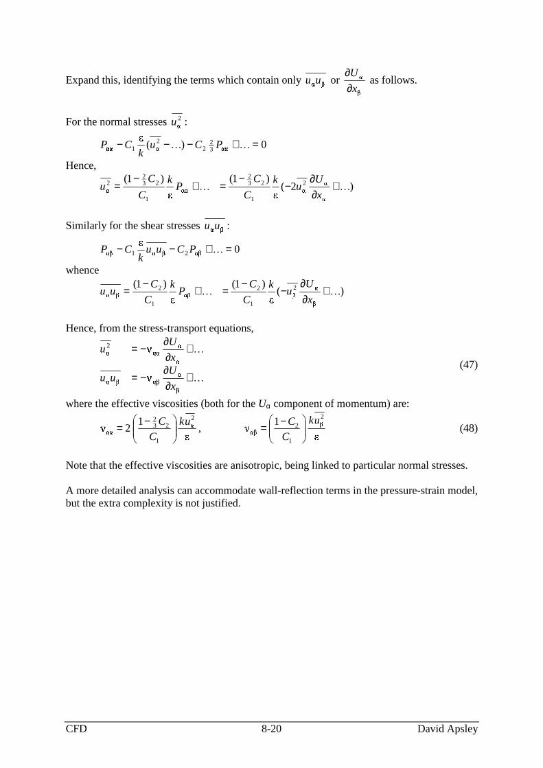
CFD 8-20 David Apsley
Expand this, identifying the terms which contain only �� uu or ��
x
U
∂∂
as follows.
For the normal stresses 2�u :
0)(�
���32
22�1��� =+−−− �� PCu
kCP
Hence,
)2(�)1(�)1(
��2�
1
232
���1
232
2� �� +∂∂
−−
=+−
=x
Uu
k
C
CP
k
C
Cu
Similarly for the shear stresses �� uu :
0�
� �2��1� � =+−− �PCuuk
CP
whence
)(�)1(�)1( � �2�
1
2� �1
2�� �� +
∂∂
−−
=+−
=x
Uu
k
C
CP
k
C
Cuu
Hence, from the stress-transport equations,
�
�
+∂∂
−=
+∂∂
−=
�
�� ���
�
����
2�
�
�
x
Uuu
x
Uu
(47)
where the effective viscosities (both for the Uα component of momentum) are:
�1�,�
12�
2�
1
2� �
2�
1
232
���uk
C
Cuk
C
C���
����
� −=���
����
� −= (48)
Note that the effective viscosities are anisotropic, being linked to particular normal stresses. A more detailed analysis can accommodate wall-reflection terms in the pressure-strain model, but the extra complexity is not justified.
CFD 8-21 David Apsley
Some References for Individual Turbulence Models Apsley, D.D., 2007, CFD calculation of turbulent flow with arbitrary wall roughness, Flow,
Turbulence and Combustion, 78, 153-175. Apsley, D.D. and Leschziner, M.A., 1998, A new low-Reynolds-number nonlinear two-
equation turbulence model for complex flows, Int. J. Heat Fluid Flow, 19, 209-222. Craft, T.J., 1998, Developments in a low-Reynolds-number second-moment closure and its
application to separating and reattaching flows, Int. J. Heat Fluid Flow, 19, 541-548. Craft, T.J., Launder, B.E. and Suga, K., 1996, Development and application of a cubic eddy-
viscosity model of turbulence, Int. J. Heat Fluid Flow, 17, 108-115. Gatski, T.B. and Speziale, C.G., 1993, On explicit algebraic stress models for complex
turbulent flows, J. Fluid Mech., 254, 59-78. Gibson, M.M. and Launder, B.E., 1978, Ground effects on pressure fluctuations in the
atmospheric boundary layer, J. Fluid Mech., 86, 491-511. Hanjali � , K., 1994, Advanced turbulence closure models: a view of current status and future
prospects, Int. J. Heat Fluid Flow, 15, 178-203. Jakirli � , S. and Hanjali � , K., 1995, A second-moment closure for non-equilibrium and
separating high- and low-Re-number flows, Proc. 10th Symp. Turbulent Shear Flows, Pennsylvania State University.
Lam, C.K.G. and Bremhorst, K.A., 1981, Modified form of the k-e model for predicting wall turbulence, Journal of Fluids Engineering, 103, 456-460.
Launder, B.E., 1989, Second-Moment Closure and its use in modelling turbulent industrial flows, Int. J. Numer. Meth. Fluids, 9, 963-985.
Launder, B.E., Reece, G.J. and Rodi, W., 1975, Progress in the development of a Reynolds-stress turbulence closure, J. Fluid Mech., 68, 537-566.
Launder, B.E. and Sharma, B.I., 1974, Application of the energy-dissipation model of turbulence to the calculation of flow near a spinning disc, Letters in Heat and Mass Transfer, 1, 131-138.
Launder, B.E. and Spalding, D.B., 1974, The numerical computation of turbulent flows, Computer Meth. Appl. Mech. Eng., 3, 269-289.
Lien, F-S. and Leschziner, M.A., 1993, Second-moment modelling of recirculating flow with a non-orthogonal collocated finite-volume algorithm, in Turbulent Shear Flows 8 (Munich, 1991), Springer-Verlag.
Menter, F.R., 1994, Two-equation eddy-viscosity turbulence models for engineering applications, AIAA J., 32, 1598-1605.
Rubinstein, R. and Barton, J.M., 1990, Nonlinear Reynolds stress models and the renormalisation group, Phys. Fluids A, 2, 1472-1476.
Speziale, C.G., 1987, On nonlinear K-l and K-� models of turbulence, J. Fluid Mech., 178,
459-475. Speziale, C.G., Sarkar, S. and Gatski, T.B., 1991, Modelling the pressure-strain correlation of
turbulence: an invariant dynamical systems approach, J. Fluid Mech., 227, 245-272. Wilcox, D.C., 1988, Reassessment of the scale-determining equation for advanced turbulence
models, AIAA J., 26, 1299-1310. Wilcox, D.C., 1988, Multi-scale model for turbulent flows, AIAA Journal, 26, 1311-1320. Wilcox, D.C., 1998, Turbulence modelling for CFD, 2nd Edition, DCW Industries. Yakhot, V., Orszag, S.A., Thangam, S., Gatski, T.B. and Speziale, C.G., 1992, Development
of turbulence models for shear flows by a double expansion technique, Phys. Fluids A, 7, 1510.
Yoshizawa, A., 1987, Statistical analysis of the derivation of the Reynolds stress from its eddy-viscosity representation, Phys. Fluids, 27, 1377-1387.