8/22/2018 2011 Transactions

http://www.amercrystalassn.org/2011-transactions-toc 1/1

Home About ACA Membership Meetings ACA RefleXions Publications Jobs/Education Awards & Prizes

Contact Us ACA History Donate Now Policy/Statements

TRANSACTIONS OF THE SYMPOSIUM HELD AT THE 2011 AMERICAN CRYSTALLOGRAPHIC ASSOCIATION ANNUAL MEETINGNew Orleans, LA

May 22 ­ June 2, 2011

Time Resolved and Charge Density ­ In Honor of Philip Coppens The ability to follow the 3D structural dynamics of photochemical processes in real time will revolutionize our understanding ofphotochemistry. The advancement of instrumentation capabilities and new light source LCLS, an x­ray free electron Laser, provides us withnew tools and techniques to conduct real time photochemistry research. It also opens up new scientific opportunities in structural dynamicstudies. This session reviewed current and future research prospects, in honor of Professor Philip Coppens' vision and leadership in thispioneering research area. Session Chairs: Peter Lee, Yu­Sheng Chen, and Jason Benedict

Table of Contents (Click on the title to download the paper)

PHASE TRANSITION DRIVEN BY LIGHT: THE KEY ROLE OF X­RAY DIFFRACTION AND TIME­RESOLVED TECHNIQUES Eric Collet, Marylise Buron, Maciej Lorenc, Marina Servol, Roman Bertoni, Ludovic Roudaut, Hiroshi Watanabe, Loic Toupet

OPTO­MAGNETIC SWITCHABLE CHARACTER IN FE(II) SPIN CROSSOVER COMPLEXES

Yu Wang, Chou­Fu Sheu, Che­Hsiu Shih, Masaki Takata DYNAMICS OF PHOTO­INDUCED PHASE SEPARATION IN SPIN CROSSOVER SOLIDS FROM TIME DEPENDENT PHOTO­CRYSTALLOGRAPHY

Sebastien Pillet, Dorothea Mader, El­Eulmi Bendeif, Gor Lebedev, William Nicolazzi, Claude Lecomte COMBINED CHARGE SPIN AND MOMENTUM DENSITIES REFINEMENT: APPLICATION TO MOLECULAR MAGNETIC MATERIALS

Claude Lecomte, Maxime Deusch, Nicolas Claiser, Mohamed Souhassou, Sebastien Pillet, Iurii Ciumacov, Beatrice Gillon, Jean Michel Gillet, Dominique Luneau DISTRIBUTED ATOMIC POLARIZABILITIES FROM ELECTRON DENSITY

Piero Macchi, Anna Krawczuk­Pantula, Daniel Pérez, Katarzyna Stadnicka CHARACTERIZATION OF WEAK INTRA­ AND INTERMOLECULAR INTERACTIONS USING EXPERIMENTAL CHARGE DENSITY DISTRIBUTIONS

Edwin Stevens

ACA more resourcesSociety Membership Publications About Crystallography

History

Bylaws Contact

Young ScientistsMember Benefits

Corporate Membership

Order FormACA PublicationsPhysics Today (AIP)

IUCr Journals

What is Crystallography? American Inst of Physics International Union of Crystallography

U.S. National Committee on Crystallography American Assoc. Crystal Growth

Powered by Fission Content Management System | Buffalo Website Design by 360 PSG

PHASE TRANSITION DRIVEN BY LIGHT: THE KEY ROLE OF X-RAY DIFFRACTION AND TIME-RESOLVED TECHNIQUES

Eric Collet, Hiroshi Watanabe, Laurent Guérin, Maciej Lorenc, Marina Servol, Loic Toupet,

Hervé Cailleau, Marylise Buron-Le Cointe Institut de Physique de Rennes, UMR UR1-CNRS Bat 11A Campus de Beaulieu, University

Rennes 1. 35042 Rennes France

The optical control of the macroscopic physical properties (magnetic, optical...) of a material by laser irradiation is gaining interest through the emerging field of photoinduced phase transitions. Light-induced changes of the macroscopic state of a material involves subtle coupling between the electronic and structural degrees of freedom, which are essential for stabilizing the photo-excited state, different in nature from the stable state. Therefore the new experimental field of photocrystallography plays a key role. This paper is reviewing different aspects of the use of this technique to investigate the nature, the mechanisms and the dynamics of photoinduced phase transitions. Crystallography coupled to laser excitation allows studying long-lived states, and time-resolved crystallography with 100 ps resolution makes it possible to catch transient states, as well a the mechanisms involved in the dynamical processes over different timescales. 1. INTRODUCTION A major challenge in physical science is the control of the physical state in a solid material on the atomic motion time-scale (100 femtosecond, 1 fs=10-15s). The femtosecond world of molecular materials represents fascinating possibilities by virtue of photoinduced co-operative and coherent changes in molecular identity, such as charge and/or spin state. Indeed, in co-operative solids the molecules are not independent and the environment of a transformed molecule is not passive but active. The structural relaxation of the electronically excited states following the simultaneous absorption of photons is no more localized on independent molecules but involves many molecules. Light may direct the functionality of a material through spectacular collective and/or cooperative photoinduced phenomena in the solid state. This can trigger the transformation of the material towards another macroscopic state of different electronic and/or structural order, for instance from non magnetic to magnetic[1], from insulator to conductor[2], from paraelectric to ferroelectric [3]. This addresses long-lived instabilities generated by cw laser excitation, as well as pulsed light driven transformations. On the one hand, cw light excitation can switch molecular states, through the trapping of the electronic excitation by structural reorganization. For some systems the live-time of the transient photoinduced state easily span over days allowing detailed analysis of the excited structure [4-8]. Light also makes it possible to reach states which can not be observed in normal thermal equilibrium conditions [1]. On the other hand, pulsed laser excitation can generate ultra-fast switching. The increase of sophisticated instrumentation, including ultra-fast time-resolved diffraction [9-18], gives fascinating capabilities not only to observe and understand the elementary dynamical processes in materials but also to watch how matter works and can be directed to a desired outcome. The key point is that in the solid state different degrees of freedom of different nature play their part

on different time scales and the pathway is complex, from the molecular to material lengths and time scales. 2. BROKEN SYMMETRY IN THE PHOTOINDUCED STATE Among switchable molecular materials, FeII spin crossover (SC) complexes have been widely

studied over the last decades:[1,6-8] the reversible low-spin (LS) high-spin (HS) switching

triggered by a change in temperature, pressure, or by light irradiation, has attracted much interest for both basic scientific understanding as well as potential technological applications in information storage or visual displays. Usually, the SC phenomenon is iso-structural. Very recently, it was demonstrated in a new material the new SC material [FeIIH2L2-Me][PF6]2 that light can drive symmetry breaking and that the photoinduced HS state generated at low temperature is different from the HS state existing at room temperature [1]. It is one of the key advantages of X-ray diffraction to be sensitive not only to the molecular structure but also to the order between the constituent molecules of the material.

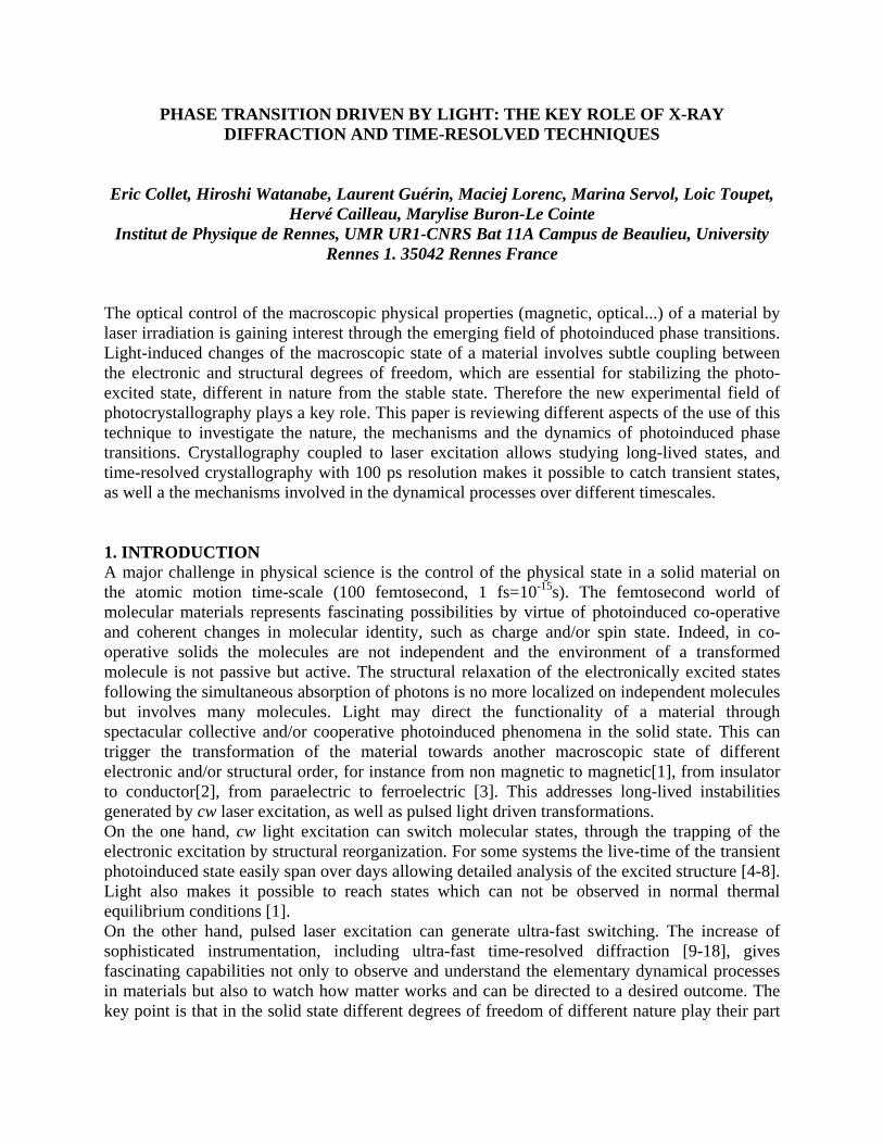
Figure 1: The photo-crystallography experimental set-up (left). The single crystal at 15 K in the He stream is excited by the laser before data collection. The change of crystal color is due to the change of electronic state between LS (violet) and HS (yellow) phases. The photo-crystallography experiment of the molecular compound [FeIIH2L2-Me][PF6]2 was performed at 15 K, after cw photo-excitation at 532 nm (Fig. 1) for generating the metastable photo-induced HS state (PIHS). The structural data were compared to the one at room temperature corresponding to the HS state existing at thermal equilibrium (Fig. 2).

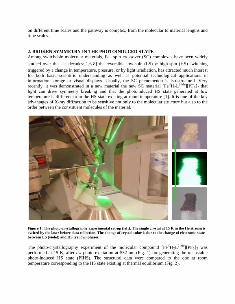
igure 2: Changes in the diffraction pattern between the HS (a) and PIHS (b) states. The broken symmetry in

iffraction data reveal different translation symmetry of the PIHS (a,b,3c) compared to the HS

h occurs upon generating the photo-induced HS phase (PIHS)

. TIME RESOLVED DIFFRACTION: DYNAMICS OF THE SPIN-STATE

ombining time-resolved optical and X-ray diffraction techniques, demonstrated

ed in Fig.3, reflects a sequence of physical processes,

. It is characterized by an elongation of <Fe-N> b

l expansion observed here through the evolution of the lattice parameter a. th.

Fthe PIHS state compared to HS state at high temperature is associated with the deformation of some molecules, associated with the loss of some 2 fold axis. D(a,b,c) state at room temperature. The structural analysis (Fig. 2) indicates that in the HT phase molecules are located on a 2 fold axis. In the PIHS phase, molecular torsion is associated with the loss of some 2 fold axis and cell triplication, resulting in a sequence of distorted and regular molecules along the c axis [1]. This symmetry breaking whicdemonstrate that different competing false ground states exist and that some of them can only be reached under non equilibrium condition by light irradiation. This is one of the important aspects of the research developed in the emerging field of photo-induced phase transitions. 3SWITCHING Recent reports cthat the switching of the spin state in a macroscopic crystal constituted of bi-stable molecules involves different mechanisms in time and space. The studies were performed in a Fe(III) solid, triggered by a femtosecond laser flash [10,11]. The ensuing dynamics span from sub-picosecond non-thermal molecular switching to microsecond diffusive heating processes through the lattice. The experiment was performed by using the optical pump / x-ray probe technique developed at the ESRF synchrotron (ID09B beamline). The existence of different steps, summarizhidden in the time domain, leaving different fingerprints for molecular transformation, cell deformation and macroscopic crystal switching:

- Step 1: local LMCT to HS relaxation cascadeond length, a well-known fingerprint of increased spin multiplicity from electron transfer to less

bonding orbitals. - Step 2: unit cel- Step 3: thermal switching characterized by an additional increase of the <Fe-N> bond leng

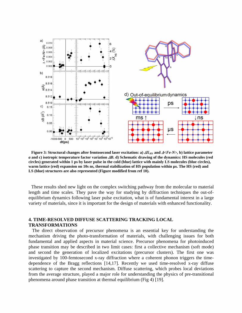
igure 3: Structural changes after femtosecond laser excitation: a) XHS and <Fe-N>, b) lattice parameter a

hese results shed new light on the complex switching pathway from the molecular to material le

. TIME-RESOLVED DIFFUSE SCATTERING TRACKING LOCAL

of precursor phenomena is an essential key for understanding the m

phenomena around phase transition at thermal equilibrium (Fig 4) [19].

F and c) isotropic temperature factor variation B. d) Schematic drawing of the dynamics: HS molecules (red

circles) generated within 1 ps by laser pulse in the cold (blue) lattice with mainly LS molecules (blue circles), warm lattice (red) expansion on 10s ns, thermal stabilization of HS population within µs. The HS (red) and LS (blue) structures are also represented (Figure modified from ref 10).

Tngth and time scales. They pave the way for studying by diffraction techniques the out-of-

equilibrium dynamics following laser pulse excitation, what is of fundamental interest in a large variety of materials, since it is important for the design of materials with enhanced functionality. 4TRANSFORMATIONS

The direct observation echanism driving the photo-transformation of materials, with challenging issues for both

fundamental and applied aspects in material science. Precursor phenomena for photoinduced phase transition may be described in two limit cases: first a collective mechanism (soft mode) and second the generation of localized excitations (precursor clusters). The first one was investigated by 100-femtosecond x-ray diffraction where a coherent phonon triggers the time-dependence of the Bragg reflections [14,17]. Recently we used time-resolved x-ray diffuse scattering to capture the second mechanism. Diffuse scattering, which probes local deviations from the average structure, played a major role for understanding the physics of pre-transitional

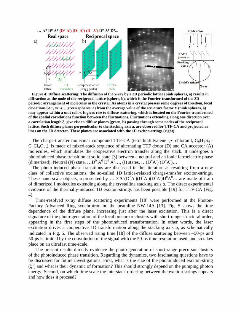
Figure 4: Diffuse scattering: The diffusion of the x-ray by a 3D periodic lattice (pink spheres, a) results in

diffraction at the node of the reciprocal lattice (sphere, b), which is the Fourier-transformed of the 3D pe l

hloranil, C6H4S4 - C Cl O ,), is made of mixed-stack sequence of alternating TTF donor (D) and CA acceptor (A) m

exciton-strings. T

ory Advanced Ring synchrotron on the beamline NW-14A [13]. Fig. 5 shows the time dep

ion. Regarding the dynamics, two fascinating questions have to be

riodic arrangement of molecules in the crystal. As atoms in a crystal possess some degrees of freedom, locadeviations (Fn=F-Fn, green spheres, a) from the average value of the structure factor F (pink spheres, a) may appear within a unit cell n. It gives rise to diffuse scattering, which is located on the Fourier-transformed of the spatial correlations function between the fluctuations. Fluctuations extending along one direction over a correlation length , give rise to diffuse planes (green, b) passing through some nodes of the reciprocal lattice. Such diffuse planes perpendicular to the stacking axis a, are observed for TTF-CA and projected as lines on the 2D detector. These planes are associated with the 1D exciton-strings (right).

The charge-transfer molecular compound TTF-CA (tetrathiafulvalene -p- c6 4 2

olecules, which stimulates the cooperative electron transfer along the stack. It undergoes a photoinduced phase transition at solid state [3] between a neutral and an ionic ferroelectric phase (dimerized). Neutral (N) state, …D0 A0 D0 A0…, (I) states, …(D+A-) (D+A-)…

The photo-induced phase transitions are discussed in the literature as resulting from a new class of collective excitations, the so-called 1D lattice-relaxed charge-transfer

hese nano-scale objects, represented by …D0A0(D+A-)(D+A-)(D+A-)D0A0… are made of train of dimerized I molecules extending along the crystalline stacking axis a. The direct experimental evidence of the thermally-induced 1D exciton-strings has been possible [19] for TTF-CA (Fig. 4).

Time-resolved x-ray diffuse scattering experiments [18] were performed at the Photon-Fact

endence of the diffuse plane, increasing just after the laser excitation. This is a direct signature of the photo-generation of the local precursor clusters with short-range structural order, appearing in the first steps of the photoinduced transformation. In other words, the laser excitation drives a cooperative 1D transformation along the stacking axis a, as schematically indicated in Fig. 5. The observed rising time [18] of the diffuse scattering between 50-ps and 50-ps is limited by the convolution of the signal with the 50-ps time resolution used, and so takes place on an ultrafast time-scale.

The present results directly evidence the photo-generation of short-range precursor clusters of the photoinduced phase transit

discussed for future investigations. First, what is the size of the photoinduced exciton-string (’) and what is their dynamic of formation? This should strongly depend on the pumping photon energy. Second, on which time scale the interstack ordering between the exciton-strings appears and how does it proceed?

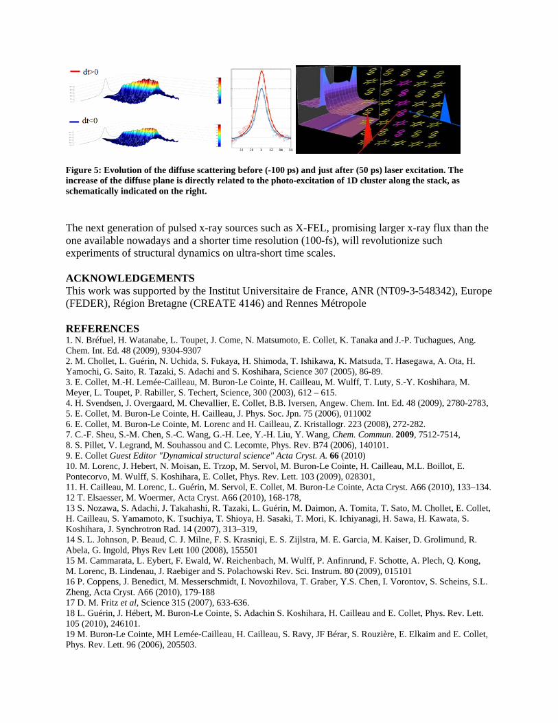
Figure 5: Evolution of the diffuse scattering before (-100 ps)

crease of the diffuse plane is directly related to the photo-e and just after (50 ps) laser excitation. The xcitation of 1D cluster along the stack, as

he next generation of pulsed x-ray sources such as X-FEL, promising larger x-ray flux than the ne available nowadays and a shorter time resolution (100-fs), will revolutionize such

his work was supported by the Institut Universitaire de France, ANR (NT09-3-548342), Europe EATE 4146) and Rennes Métropole

. N. Bréfuel, H. Watanabe, L. Toupet, J. Come, N. Matsumoto, E. Collet, K. Tanaka and J.-P. Tuchagues, Ang. 09), 9304-9307

83,

–134.

.

inschematically indicated on the right. Toexperiments of structural dynamics on ultra-short time scales. ACKNOWLEDGEMENTS T(FEDER), Région Bretagne (CR REFERENCES 1Chem. Int. Ed. 48 (202. M. Chollet, L. Guérin, N. Uchida, S. Fukaya, H. Shimoda, T. Ishikawa, K. Matsuda, T. Hasegawa, A. Ota, H. Yamochi, G. Saito, R. Tazaki, S. Adachi and S. Koshihara, Science 307 (2005), 86-89. 3. E. Collet, M.-H. Lemée-Cailleau, M. Buron-Le Cointe, H. Cailleau, M. Wulff, T. Luty, S.-Y. Koshihara, M. Meyer, L. Toupet, P. Rabiller, S. Techert, Science, 300 (2003), 612 – 615. 4. H. Svendsen, J. Overgaard, M. Chevallier, E. Collet, B.B. Iversen, Angew. Chem. Int. Ed. 48 (2009), 2780-275. E. Collet, M. Buron-Le Cointe, H. Cailleau, J. Phys. Soc. Jpn. 75 (2006), 011002 6. E. Collet, M. Buron-Le Cointe, M. Lorenc and H. Cailleau, Z. Kristallogr. 223 (2008), 272-282.

mun. 2009, 7512-7514, 7. C.-F. Sheu, S.-M. Chen, S.-C. Wang, G.-H. Lee, Y.-H. Liu, Y. Wang, Chem. Com8. S. Pillet, V. Legrand, M. Souhassou and C. Lecomte, Phys. Rev. B74 (2006), 140101. 9. E. Collet Guest Editor "Dynamical structural science" Acta Cryst. A. 66 (2010)

au, M.L. Boillot, E. 10. M. Lorenc, J. Hebert, N. Moisan, E. Trzop, M. Servol, M. Buron-Le Cointe, H. Caille, Pontecorvo, M. Wulff, S. Koshihara, E. Collet, Phys. Rev. Lett. 103 (2009), 028301

11. H. Cailleau, M. Lorenc, L. Guérin, M. Servol, E. Collet, M. Buron-Le Cointe, Acta Cryst. A66 (2010), 13312 T. Elsaesser, M. Woermer, Acta Cryst. A66 (2010), 168-178, 13 S. Nozawa, S. Adachi, J. Takahashi, R. Tazaki, L. Guérin, M. Daimon, A. Tomita, T. Sato, M. Chollet, E. Collet,

ori, K. Ichiyanagi, H. Sawa, H. Kawata, S. H. Cailleau, S. Yamamoto, K. Tsuchiya, T. Shioya, H. Sasaki, T. MKoshihara, J. Synchrotron Rad. 14 (2007), 313–319, 14 S. L. Johnson, P. Beaud, C. J. Milne, F. S. Krasniqi, E. S. Zijlstra, M. E. Garcia, M. Kaiser, D. Grolimund, R. Abela, G. Ingold, Phys Rev Lett 100 (2008), 155501 15 M. Cammarata, L. Eybert, F. Ewald, W. Reichenbach, M. Wulff, P. Anfinrund, F. Schotte, A. Plech, Q. Kong, M. Lorenc, B. Lindenau, J. Raebiger and S. Polachowski Rev. Sci. Instrum. 80 (2009), 015101 16 P. Coppens, J. Benedict, M. Messerschmidt, I. Novozhilova, T. Graber, Y.S. Chen, I. Vorontov, S. Scheins, S.LZheng, Acta Cryst. A66 (2010), 179-188 17 D. M. Fritz et al, Science 315 (2007), 633-636. 18 L. Guérin, J. Hébert, M. Buron-Le Cointe, S. Adachin S. Koshihara, H. Cailleau and E. Collet, Phys. Rev. Lett. 105 (2010), 246101. 19 M. Buron-Le Cointe, MH Lemée-Cailleau, H. Cailleau, S. Ravy, JF Bérar, S. Rouzière, E. Elkaim and E. Collet,Phys. Rev. Lett. 96 (2006), 205503.

OPTO-MAGNETIC SWITCHABLE CHARACTER IN FE(II) SPIN CROSSOVER

COMPLEXES

Yu Wang, Chou-Fu Sheu and Lai-Chin Wu

Department of Chemistry National Taiwan University, No. 1, Sec. 4, Roosevelt Road, Taipei

10617, Taiwan

Che-Hsiu Shih and Masaki Takata

Department of Advanced Materials Science, University of Tokyo, Kashiwa, Chiba 277-8561,

Japan

RIKEN SPring-8 center, Sayo, Hyogo 679-5148, Japan

Jey-Jau Lee

National Synchrotron Radiation Research Center, Hsin-Chu, Taiwan

Yu-Sheng Chen

CARS / Univ. of Chicago, IL 60637, USA

It is well known that octahedral coordinated Fe (II) complexes with proper ligands often exhibit

spin transition under external stimuli, such as temperature, pressure, light irradiation or even the

change of solvents. A simple abrupt transition at transition temperature will make clearly a

magnetic switch from a paramagnetic species with Fe(II) at high spin (HS) quintet state (5T2) to a

diamagnetic one at low spin (LS) singlet state (1A1) or vice versa. Typical structural changes are

often accompanied to such transition; structural magnetic relationship is established for some

very complicated magnetic behaviors. The LS to HS transition or in some rare cases, from HS to

LS could be induced by light irradiation with proper wavelength, often at extreme low

temperature, say below 50K; a so called light induced excited spin state trapping (LIESST) or a

reverse LIESST phenomenon. Examples will be given with a few Fe complexes with

triazole-containing ligands; property changes due to the light irradiation can be monitored by ir,

magnetic susceptibility, Fe K- or L-edge x-ray absorption as well as the x-ray diffraction.

Polymorphism and order-disorder of the structures are additional interests on these complexes;

which give rise to even richer property related aspects.

1. INTRODUCTION

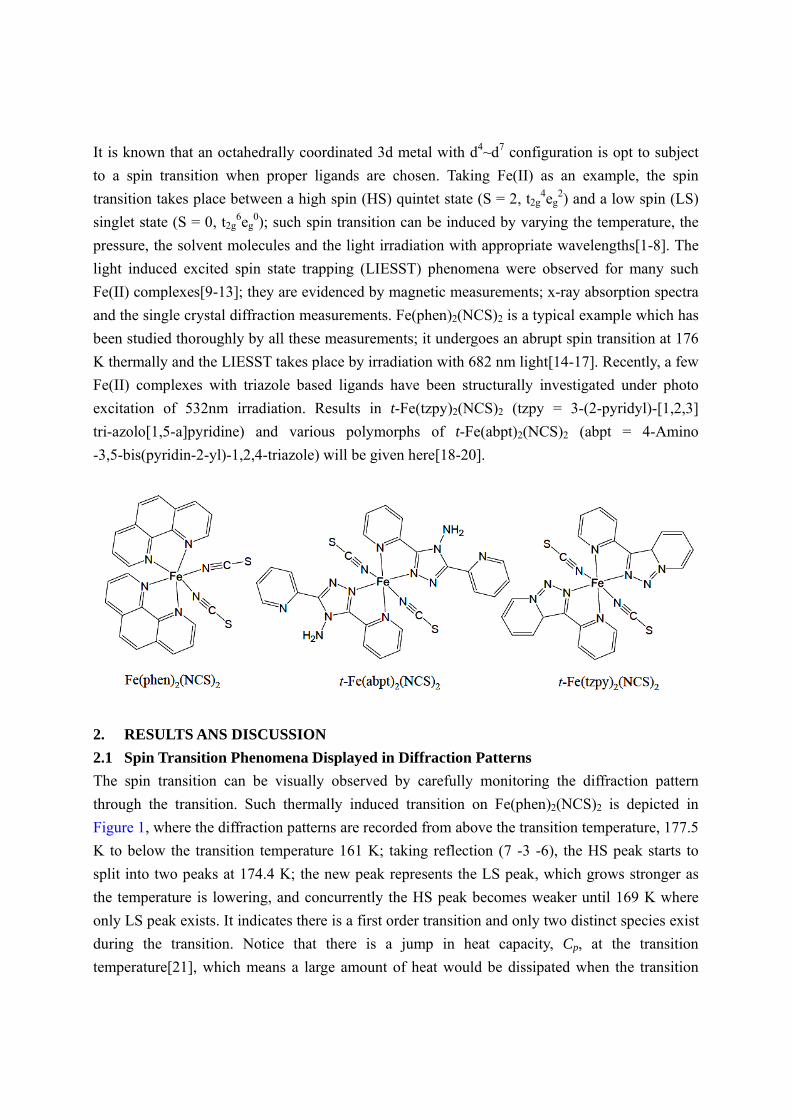
It is known that an octahedrally coordinated 3d metal with d4~d7 configuration is opt to subject

to a spin transition when proper ligands are chosen. Taking Fe(II) as an example, the spin

transition takes place between a high spin (HS) quintet state (S = 2, t2g4eg

2) and a low spin (LS)

singlet state (S = 0, t2g6eg

0); such spin transition can be induced by varying the temperature, the

pressure, the solvent molecules and the light irradiation with appropriate wavelengths[1-8]. The

light induced excited spin state trapping (LIESST) phenomena were observed for many such

Fe(II) complexes[9-13]; they are evidenced by magnetic measurements; x-ray absorption spectra

and the single crystal diffraction measurements. Fe(phen)2(NCS)2 is a typical example which has

been studied thoroughly by all these measurements; it undergoes an abrupt spin transition at 176

K thermally and the LIESST takes place by irradiation with 682 nm light[14-17]. Recently, a few

Fe(II) complexes with triazole based ligands have been structurally investigated under photo

excitation of 532nm irradiation. Results in t-Fe(tzpy)2(NCS)2 (tzpy = 3-(2-pyridyl)-[1,2,3]

tri-azolo[1,5-a]pyridine) and various polymorphs of t-Fe(abpt)2(NCS)2 (abpt = 4-Amino

-3,5-bis(pyridin-2-yl)-1,2,4-triazole) will be given here[18-20].

2. RESULTS ANS DISCUSSION

2.1 Spin Transition Phenomena Displayed in Diffraction Patterns

The spin transition can be visually observed by carefully monitoring the diffraction pattern

through the transition. Such thermally induced transition on Fe(phen)2(NCS)2 is depicted in

Figure 1, where the diffraction patterns are recorded from above the transition temperature, 177.5

K to below the transition temperature 161 K; taking reflection (7 -3 -6), the HS peak starts to

split into two peaks at 174.4 K; the new peak represents the LS peak, which grows stronger as

the temperature is lowering, and concurrently the HS peak becomes weaker until 169 K where

only LS peak exists. It indicates there is a first order transition and only two distinct species exist

during the transition. Notice that there is a jump in heat capacity, Cp, at the transition

temperature[21], which means a large amount of heat would be dissipated when the transition

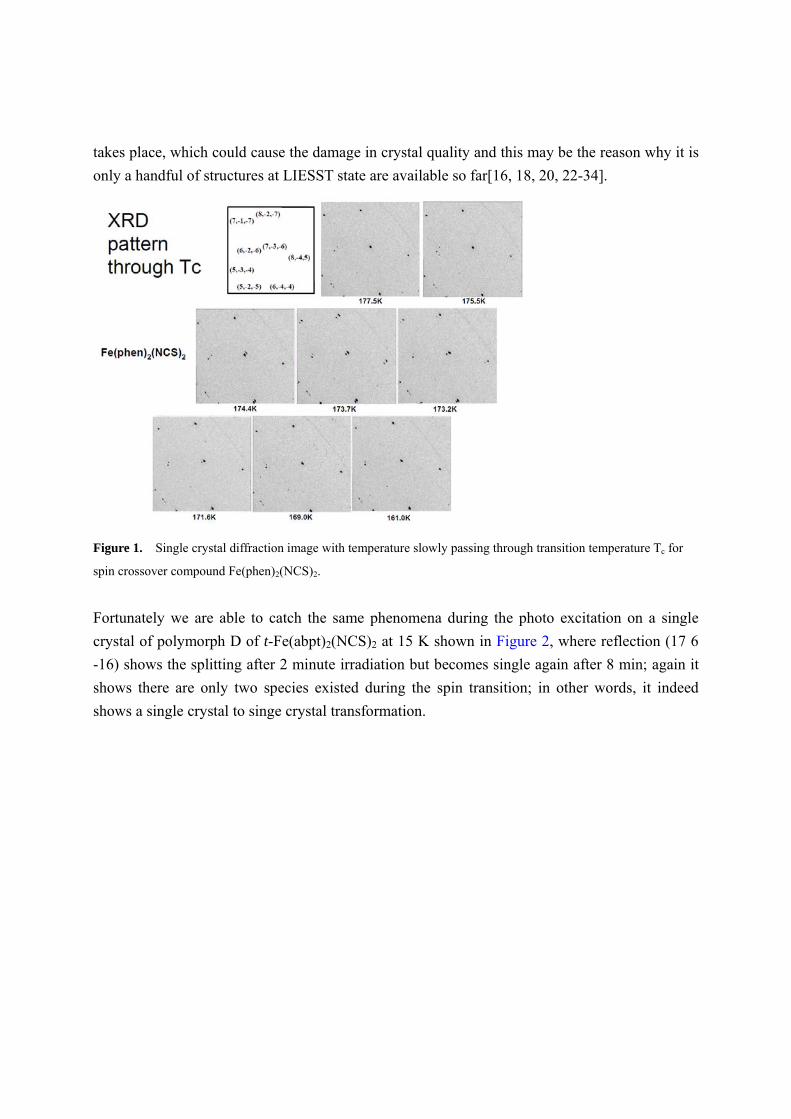
takes place, which could cause the damage in crystal quality and this may be the reason why it is

only a handful of structures at LIESST state are available so far[16, 18, 20, 22-34].

Figure 1. Single crystal diffraction image with temperature slowly passing through transition temperature Tc for

spin crossover compound Fe(phen)2(NCS)2.

Fortunately we are able to catch the same phenomena during the photo excitation on a single

crystal of polymorph D of t-Fe(abpt)2(NCS)2 at 15 K shown in Figure 2, where reflection (17 6

-16) shows the splitting after 2 minute irradiation but becomes single again after 8 min; again it

shows there are only two species existed during the spin transition; in other words, it indeed

shows a single crystal to singe crystal transformation.

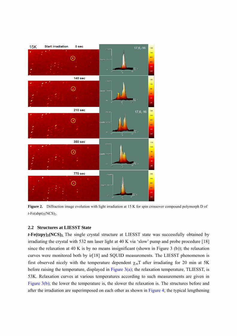
Figure 2. Diffraction image evolution with light irradiation at 15 K for spin crossover compound polymorph D of

t-Fe(abpt)2(NCS)2.

2.2 Structures at LIESST State

t-Fe(tzpy)2(NCS)2. The single crystal structure at LIESST state was successfully obtained by

irradiating the crystal with 532 nm laser light at 40 K via ‘slow’ pump and probe procedure [18]

since the relaxation at 40 K is by no means insignificant (shown in Figure 3 (b)); the relaxation

curves were monitored both by ir[18] and SQUID measurements. The LIESST phenomenon is

first observed nicely with the temperature dependent mT after irradiating for 20 min at 5K

before raising the temperature, displayed in Figure 3(a); the relaxation temperature, TLIESST, is

53K. Relaxation curves at various temperatures according to such measurements are given in

Figure 3(b); the lower the temperature is, the slower the relaxation is. The structures before and

after the irradiation are superimposed on each other as shown in Figure 4; the typical lengthening

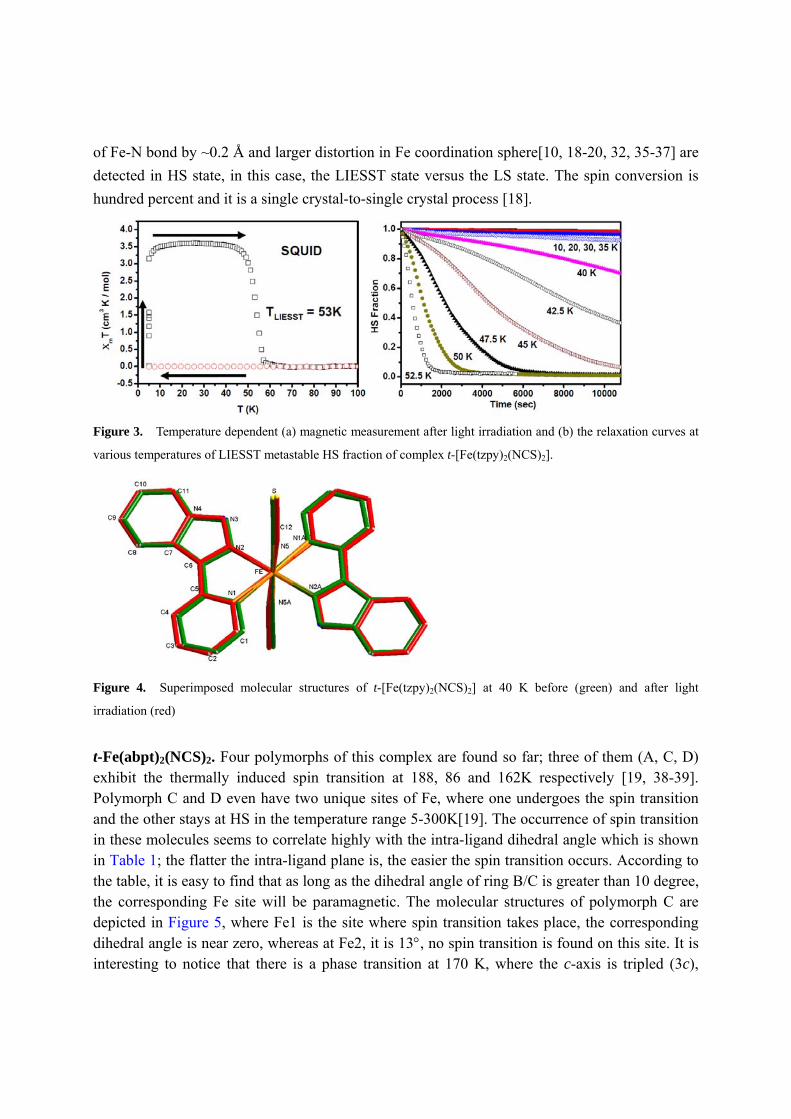
of Fe-N bond by ~0.2 Å and larger distortion in Fe coordination sphere[10, 18-20, 32, 35-37] are

detected in HS state, in this case, the LIESST state versus the LS state. The spin conversion is

hundred percent and it is a single crystal-to-single crystal process [18].

Figure 3. Temperature dependent (a) magnetic measurement after light irradiation and (b) the relaxation curves at

various temperatures of LIESST metastable HS fraction of complex t-[Fe(tzpy)2(NCS)2].

Figure 4. Superimposed molecular structures of t-[Fe(tzpy)2(NCS)2] at 40 K before (green) and after light

irradiation (red)

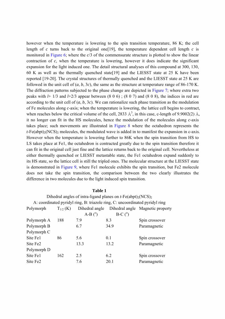
t-Fe(abpt)2(NCS)2. Four polymorphs of this complex are found so far; three of them (A, C, D) exhibit the thermally induced spin transition at 188, 86 and 162K respectively [19, 38-39]. Polymorph C and D even have two unique sites of Fe, where one undergoes the spin transition and the other stays at HS in the temperature range 5-300K[19]. The occurrence of spin transition in these molecules seems to correlate highly with the intra-ligand dihedral angle which is shown in Table 1; the flatter the intra-ligand plane is, the easier the spin transition occurs. According to the table, it is easy to find that as long as the dihedral angle of ring B/C is greater than 10 degree, the corresponding Fe site will be paramagnetic. The molecular structures of polymorph C are depicted in Figure 5, where Fe1 is the site where spin transition takes place, the corresponding dihedral angle is near zero, whereas at Fe2, it is 13, no spin transition is found on this site. It is interesting to notice that there is a phase transition at 170 K, where the c-axis is tripled (3c),

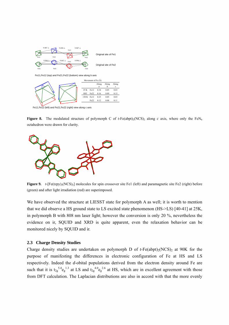
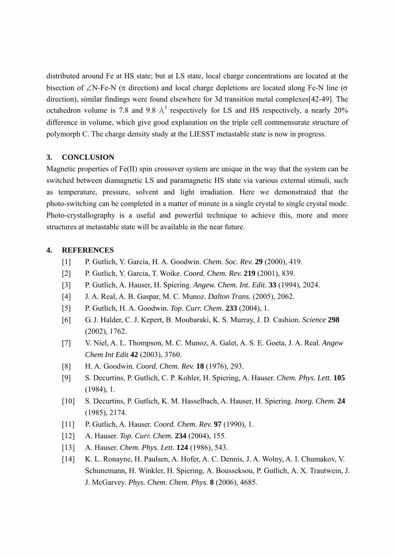
however when the temperature is lowering to the spin transition temperature, 86 K; the cell length of c turns back to the original one[19], the temperature dependent cell length c is monitored in Figure 6; where the c/3 of the commensurate structure is plotted to show the linear contraction of c, when the temperature is lowering, however it does indicate the significant expansion for the light induced one. The detail structural analyses of this compound at 300, 130, 60 K as well as the thermally quenched state[19] and the LIESST state at 25 K have been reported [19-20]. The crystal structures of thermally quenched and the LIESST state at 25 K are followed in the unit cell of (a, b, 3c), the same as the structure at temperature range of 86-170 K. The diffraction patterns subjected to the phase change are depicted in Figure 7; where extra two peaks with l+ 1/3 and l+2/3 appear between (8 0 6) ; (8 0 7) and (8 0 8), the indices in red are according to the unit cell of (a, b, 3c). We can rationalize such phase transition as the modulation of Fe molecules along c-axis; when the temperature is lowering, the lattice cell begins to contract, when reaches below the critical volume of the cell, 2833 Å3, in this case, c-length of 9.9002(2) Å, it no longer can fit in the HS molecules, hence the modulation of the molecules along c-axis takes place; such movements are illustrated in Figure 8 where the octahedron represents the t-Fe(abpt)2(NCS)2 molecules, the modulated wave is added in to manifest the expansion in c-axis. However when the temperature is lowering further to 86K when the spin transition from HS to LS takes place at Fe1, the octahedron is contracted greatly due to the spin transition therefore it can fit in the original cell just fine and the lattice returns back to the original cell. Nevertheless at either thermally quenched or LIESST metastable state, the Fe1 octahedron expand suddenly to its HS state, so the lattice cell is still the tripled ones. The molecular structure at the LIESST state is demonstrated in Figure 9, where Fe1 molecule exhibits the spin transition, but Fe2 molecule does not take the spin transition, the comparison between the two clearly illustrates the difference in two molecules due to the light induced spin transition.

Table 1 Dihedral angles of intra-ligand planes on t-Fe(abpt)2(NCS)2

A: coordinated pyridyl ring, B: triazole ring, C: uncoordinated pyridyl ring Polymorph T1/2 (K) Dihedral angle

A-B (o) Dihedral angle

B-C (o) Magnetic property

Polymorph A 188 7.9 8.3 Spin crossover Polymorph B 6.7 34.9 Paramagnetic Polymorph C Site Fe1 86 5.6 0.1 Spin crossover Site Fe2 13.3 13.2 Paramagnetic Polymorph D Site Fe1 162 2.5 6.2 Spin crossover Site Fe2 7.6 20.1 Paramagnetic

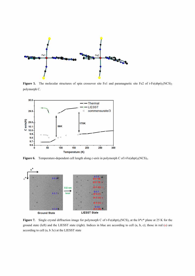
Figure 5. The molecular structures of spin crossover site Fe1 and paramagnetic site Fe2 of t-Fe(abpt)2(NCS)2

polymorph C.

Figure 6. Temperature-dependent cell length along c-axis in polymorph C of t-Fe(abpt)2(NCS)2.

Figure 7. Single crystal diffraction image for polymorph C of t-Fe(abpt)2(NCS)2 at the b*c* plane at 25 K for the

ground state (left) and the LIESST state (right). Indices in blue are according to cell (a, b, c); those in red (o) are

according to cell (a, b 3c) at the LIESST state

Movement of Fe (Ǻ)

130 K

HS3

25 K 0.030.050.34Fe12

0.150.090.16Fe22

0.110.080.12Fe22

0.030.050.25Fe12

Along c

Along b

Along a

Fe11,Fe12 (left) and Fe21,Fe22 (right) view along c axis

Fe11,Fe12 (top) and Fe21,Fe22 (bottom) view along b axis

9.907 Å 9.850 Å 9.907 Å

9.994 Å 9.663 Å 9.994 Å

Original site of Fe1

Original site of Fe2

Fe11 Fe12

Fe12

Fe11

Fe21 Fe21Fe22

Fe22

Figure 8. The modulated structure of polymorph C of t-Fe(abpt)2(NCS)2 along c axis, where only the FeN6

octahedron were drawn for clarity.

Figure 9. t-[Fe(tzpy)2(NCS)2] molecules for spin crossover site Fe1 (left) and paramagnetic site Fe2 (right) before

(green) and after light irradiation (red) are superimposed.

We have observed the structure at LIESST state for polymorph A as well; it is worth to mention

that we did observe a HS ground state to LS excited state phenomenon (HS->LS) [40-41] at 25K,

in polymorph B with 808 nm laser light; however the conversion is only 20 %, nevertheless the

evidence on ir, SQUID and XRD is quite apparent, even the relaxation behavior can be

monitored nicely by SQUID and ir.

2.3 Charge Density Studies

Charge density studies are undertaken on polymorph D of t-Fe(abpt)2(NCS)2 at 90K for the

purpose of manifesting the differences in electronic configuration of Fe at HS and LS

respectively. Indeed the d-obital populations derived from the electron density around Fe are

such that it is t2g5.4eg

1.3 at LS and t2g4.0eg

2.6 at HS, which are in excellent agreement with those

from DFT calculation. The Laplacian distributions are also in accord with that the more evenly

distributed around Fe at HS state; but at LS state, local charge concentrations are located at the

bisection of N-Fe-N ( direction) and local charge depletions are located along Fe-N line (

direction), similar findings were found elsewhere for 3d transition metal complexes[42-49]. The

octahedron volume is 7.8 and 9.8 Å3 respectively for LS and HS respectively, a nearly 20%

difference in volume, which give good explanation on the triple cell commensurate structure of

polymorph C. The charge density study at the LIESST metastable state is now in progress.

3. CONCLUSION

Magnetic properties of Fe(II) spin crossover system are unique in the way that the system can be

switched between diamagnetic LS and paramagnetic HS state via various external stimuli, such

as temperature, pressure, solvent and light irradiation. Here we demonstrated that the

photo-switching can be completed in a matter of minute in a single crystal to single crystal mode.

Photo-crystallography is a useful and powerful technique to achieve this, more and more

structures at metastable state will be available in the near future.

4. REFERENCES

[1] P. Gutlich, Y. Garcia, H. A. Goodwin. Chem. Soc. Rev. 29 (2000), 419.

[2] P. Gutlich, Y. Garcia, T. Woike. Coord. Chem. Rev. 219 (2001), 839.

[3] P. Gutlich, A. Hauser, H. Spiering. Angew. Chem. Int. Edit. 33 (1994), 2024.

[4] J. A. Real, A. B. Gaspar, M. C. Munoz. Dalton Trans. (2005), 2062.

[5] P. Gutlich, H. A. Goodwin. Top. Curr. Chem. 233 (2004), 1.

[6] G. J. Halder, C. J. Kepert, B. Moubaraki, K. S. Murray, J. D. Cashion. Science 298

(2002), 1762.

[7] V. Niel, A. L. Thompson, M. C. Munoz, A. Galet, A. S. E. Goeta, J. A. Real. Angew

Chem Int Edit 42 (2003), 3760.

[8] H. A. Goodwin. Coord. Chem. Rev. 18 (1976), 293.

[9] S. Decurtins, P. Gutlich, C. P. Kohler, H. Spiering, A. Hauser. Chem. Phys. Lett. 105

(1984), 1.

[10] S. Decurtins, P. Gutlich, K. M. Hasselbach, A. Hauser, H. Spiering. Inorg. Chem. 24

(1985), 2174.

[11] P. Gutlich, A. Hauser. Coord. Chem. Rev. 97 (1990), 1.

[12] A. Hauser. Top. Curr. Chem. 234 (2004), 155.

[13] A. Hauser. Chem. Phys. Lett. 124 (1986), 543.

[14] K. L. Ronayne, H. Paulsen, A. Hofer, A. C. Dennis, J. A. Wolny, A. I. Chumakov, V.

Schunemann, H. Winkler, H. Spiering, A. Bousseksou, P. Gutlich, A. X. Trautwein, J.

J. McGarvey. Phys. Chem. Chem. Phys. 8 (2006), 4685.

[15] J. J. Lee, H. S. Sheu, C. R. Lee, J. M. Chen, J. F. Lee, C. C. Wang, C. H. Huang, Y.

Wang. J. Am. Chem. Soc. 122 (2000), 5742.

[16] M. Marchivie, P. Guionneau, J. A. K. Howard, G. Chastanet, J. F. Letard, A. E.

Goeta, D. Chasseau. J. Am. Chem. Soc. 124 (2002), 194.

[17] E. Konig, K. Madeja. Chem. Commun. (1966), 61.

[18] C. F. Sheu, K. Chen, S. M. Chen, Y. S. Wen, G. H. Lee, J. M. Chen, J. F. Lee, B. M.

Cheng, H. S. Sheu, N. Yasuda, Y. Ozawa, K. Toriumi, Y. Wang. Chem. Eur. J. 15

(2009), 2384.

[19] C. F. Sheu, S. M. Chen, S. C. Wang, G. H. Lee, Y. H. Liu, Y. Wang. Chem. Commun.

(2009), 7512.

[20] C. H. Shih, C. F. Sheu, K. Kato, K. Sugimoto, J. Kim, Y. Wang, M. Takata. Dalton

Trans. 39 (2010), 9794.

[21] M. Sorai, S. Seki. J. Phys. Soc. Jpn. 33 (1972), 575.

[22] N. Huby, L. Guerin, E. Collet, L. Toupet, J. C. Ameline, H. Cailleau, T. Roisnel, T.

Tayagaki, K. Tanaka. Phys. Rev. B 69 (2004), 020101(R).

[23] J. Kusz, D. Schollmeyer, H. Spiering, P. Gutlich. J. Appl. Crystallogr. 38 (2005),

528.

[24] V. Legrand, S. Pillet, C. Carbonera, M. Souhassou, J. F. Letard, P. Guionneau, C.

Lecomte. Eur. J. Inorg. Chem. (2007), 5693.

[25] V. Legrand, S. Pillet, H. P. Weber, M. Souhassou, J. F. Letard, P. Guionneau, C.

Lecomte. J. Appl. Crystallogr. 40 (2007), 1076.

[26] E. J. MacLean, C. M. McGrath, C. J. O'Connor, C. Sangregorio, J. M. W. Seddon, E.

Sinn, F. E. Sowrey, S. L. Teat, A. E. Terry, G. B. M. Vaughan, N. A. Young. Chem.

Eur. J. 9 (2003), 5314.

[27] A. L. Thompson, A. E. Goeta, J. A. Real, A. Galet, M. C. Munoz. Chem. Commun.

(2004), 1390.

[28] V. Niel, A. L. Thompson, A. E. Goeta, C. Enachescu, A. Hauser, A. Galet, M. C.

Munoz, J. A. Real. Chem. Eur. J. 11 (2005), 2047.

[29] K. Ichiyanagi, J. Hebert, L. Toupet, H. Cailleau, P. Guionneau, J. F. Letard, E. Collet.

Phys. Rev. B 73 (2006), 060408.

[30] V. A. Money, I. R. Evans, M. A. Halcrow, A. E. Goeta, J. A. K. Howard. Chem.

Commun. (2003), 158.

[31] V. A. Money, J. Elhaik, M. A. Halcrow, J. A. K. Howard. Dalton Trans. (2004),

1516.

[32] C. F. Sheu, S. Pillet, Y. C. Lin, S. M. Chen, I. J. Hsu, C. Lecomte, Y. Wang. Inorg.

Chem. 47 (2008), 10866.

[33] E. Trzop, M. B. L. Cointe, H. Cailleau, L. Toupet, G. Molnar, A. Bousseksou, A. B.

Gaspar, J. A. Real, E. Collet. J. Appl. Crystallogr. 40 (2007), 158.

[34] J. Kusz, H. Spiering, P. Gutlich. J. Appl. Crystallogr. 34 (2001), 229.

[35] M. Marchivie, P. Guionneau, J. F. Letard, D. Chasseau. Acta Crystallogr. B 61

(2005), 25.

[36] P. Guionneau, M. Marchivie, G. Bravic, J. F. Letard, D. Chasseau. J. Mater. Chem.

12 (2002), 2546.

[37] P. Guionneau, C. Brigouleix, Y. Barrans, A. E. Goeta, J. F. Letard, J. A. K. Howard, J.

Gaultier, D. Chasseau. C. R. Acad. Sci., Ser. IIc: Chim. 4 (2001), 161.

[38] A. B. Gaspar, M. C. Munoz, N. Moliner, V. Ksenofontov, G. Levchenko, P. Gutlich,

J. A. Real. Monatsh. Chem. 134 (2003), 285.

[39] N. Moliner, M. C. Munoz, S. Letard, J. F. Letard, X. Solans, R. Burriel, M. Castro,

O. Kahn, J. A. Real. Inorg. Chim. Acta 291 (1999), 279.

[40] P. Gutlich, P. Poganiuch. Angew. Chem. Int. Edit. 30 (1991), 975.

[41] P. Poganiuch, S. Decurtins, P. Gutlich. J. Am. Chem. Soc. 112 (1990), 3270.

[42] V. Legrand, S. Pillet, M. Souhassou, N. Lugan, C. Lecomte. J. Am. Chem. Soc. 128

(2006), 13921.

[43] S. Pillet, V. Legrand, H. P. Weber, M. Souhassou, J. F. Letard, P. Guionneau, C.

Lecomte. Z. Kristallogr. 223 (2008), 235.

[44] T. S. Hwang, Y. Wang. J. Phys. Chem. A 102 (1998), 3726.

[45] L. E. Johnson, D. B. DuPre. J. Phys. Chem. A 113 (2009), 8647.

[46] C. R. Lee, L. Y. Tan, Y. Wang. , J. Phys. Chem. Solids, 62 (2001), 1613.

[47] J. J. Lee, G. H. Lee, Y. Wang. Chem. Eur. J. (2002), 1821.

[48] P. Macchi, A. Sironi. Coord. Chem. Rev. 238 (2003), 383.

[49] C. R. Lee, C. C. Wang, K. C. Chen, G. H. Lee, Y. Wang. , J. Phys. Chem. A, 103

(1999), 156.

DYNAMICS OF PHOTO-INDUCED PHASE SEPARATION IN SPIN CROSSOVER SOLIDS FROM TIME DEPENDENT PHOTO-CRYSTALLOGRAPHY

Sébastien Pillet,1 Gor Lebedev1,2 and William Nicolazzi1,3 1 Laboratoire de Cristallographie, Résonance Magnétique et Modélisations, UMR CNRS 7036,

Institut Jean Barriol, Nancy-Université, BP239, 54506 Vandoeuvre les Nancy, France. 2 present address : CEA, LETI, MINATEC Campus, Grenoble, France

3 present address : Laboratoire de Chimie de Coordination, CNRS UPR-8241, Université de Toulouse, UPS, INP, F-31077 Toulouse, France

1. ABSTRACT The use of time/temperature dependent x-ray photo-crystallographic technique to investigate the dynamics of solid state spin transition is illustrated, and combined with Monte-Carlo simulations of a microscopic elastic Ising-like model. Specifically, the kinetics of light-induced spin transition and relaxation in [FexZn1-x(phen)2(NCS)2] (phen=1,10-phenanthroline) is reported from kinetic x-ray powder diffraction at variable temperature with in situ optical excitation. It is shown that the light-induced phase transformation and subsequent thermal relaxation is driven by a heterogeneous nucleation and growth mechanism with phase separation. The high spin to low spin isothermal relaxation curves strongly differ from first-order kinetics, and are interpreted using the Kolmogorov-Johnson-Mehl-Avrami model of phase transformation, from which the activation energy to domain growth is derived. The dynamics of such photoinduced phase transition may well be appreciated using kinetic numerical simulations of a microscopic two-variable model with appropriate computation of the corresponding diffraction pattern. A comparative analysis of the experimental and simulated diffraction pattern with excitation duration and intensity as variables is performed. 2. INTRODUCTION The thorough description of structural reorganizations in solids undergoing phase transformations is of fundamental importance. Of prime interest are cases for which the phase transformation can be triggered by external stimuli, e.g. light, pressure, electric field, so that a direct control of the properties of such materials may be achieved. In this context, single crystal and powder x-ray diffraction under optical excitation, termed photocrystallography, is an essential technique which allows getting a clear structural description of the molecular and crystal lattice response to optical perturbation. Indeed, many solid-state processes can be triggered or driven by light which renders this technique very appealing for the study of out-of-equilibrium phenomena such as structural relaxation processes [1], long-lived metastable states [2], short-lived excited states [3,4] and solid-state photochemical reactions [5,6]. The recent achievements in time resolved x-ray monochromatic [7,8] or polychromatic Laue [9] diffraction have clearly open new exciting possibilities in the ultra-fast regime in combination to the emerging field of x-ray transient absorption spectroscopy [10]. The choice of suitable excitation conditions in terms of wavelength, bandwidth (broad-band or monochromatic), power and duration is a pre-requisite for

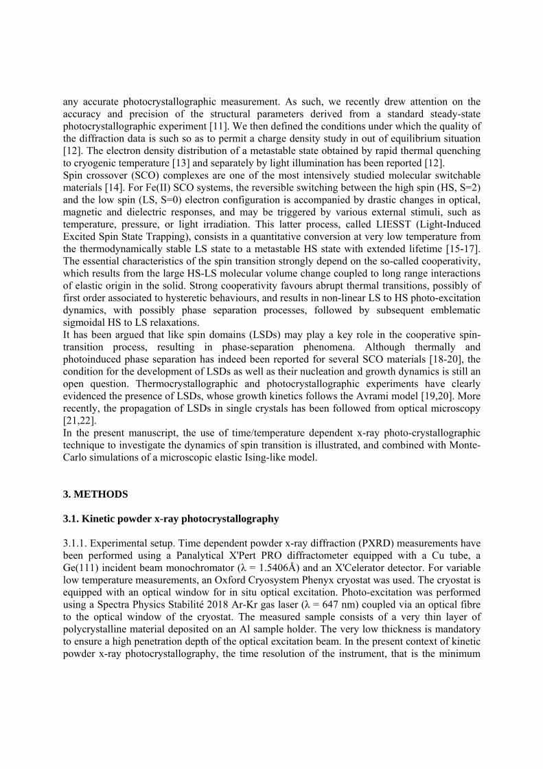
any accurate photocrystallographic measurement. As such, we recently drew attention on the accuracy and precision of the structural parameters derived from a standard steady-state photocrystallographic experiment [11]. We then defined the conditions under which the quality of the diffraction data is such so as to permit a charge density study in out of equilibrium situation [12]. The electron density distribution of a metastable state obtained by rapid thermal quenching to cryogenic temperature [13] and separately by light illumination has been reported [12]. Spin crossover (SCO) complexes are one of the most intensively studied molecular switchable materials [14]. For Fe(II) SCO systems, the reversible switching between the high spin (HS, S=2) and the low spin (LS, S=0) electron configuration is accompanied by drastic changes in optical, magnetic and dielectric responses, and may be triggered by various external stimuli, such as temperature, pressure, or light irradiation. This latter process, called LIESST (Light-Induced Excited Spin State Trapping), consists in a quantitative conversion at very low temperature from the thermodynamically stable LS state to a metastable HS state with extended lifetime [15-17]. The essential characteristics of the spin transition strongly depend on the so-called cooperativity, which results from the large HS-LS molecular volume change coupled to long range interactions of elastic origin in the solid. Strong cooperativity favours abrupt thermal transitions, possibly of first order associated to hysteretic behaviours, and results in non-linear LS to HS photo-excitation dynamics, with possibly phase separation processes, followed by subsequent emblematic sigmoidal HS to LS relaxations. It has been argued that like spin domains (LSDs) may play a key role in the cooperative spin-transition process, resulting in phase-separation phenomena. Although thermally and photoinduced phase separation has indeed been reported for several SCO materials [18-20], the condition for the development of LSDs as well as their nucleation and growth dynamics is still an open question. Thermocrystallographic and photocrystallographic experiments have clearly evidenced the presence of LSDs, whose growth kinetics follows the Avrami model [19,20]. More recently, the propagation of LSDs in single crystals has been followed from optical microscopy [21,22]. In the present manuscript, the use of time/temperature dependent x-ray photo-crystallographic technique to investigate the dynamics of spin transition is illustrated, and combined with Monte-Carlo simulations of a microscopic elastic Ising-like model. 3. METHODS 3.1. Kinetic powder x-ray photocrystallography 3.1.1. Experimental setup. Time dependent powder x-ray diffraction (PXRD) measurements have been performed using a Panalytical X'Pert PRO diffractometer equipped with a Cu tube, a Ge(111) incident beam monochromator (λ = 1.5406Å) and an X'Celerator detector. For variable low temperature measurements, an Oxford Cryosystem Phenyx cryostat was used. The cryostat is equipped with an optical window for in situ optical excitation. Photo-excitation was performed using a Spectra Physics Stabilité 2018 Ar-Kr gas laser (λ = 647 nm) coupled via an optical fibre to the optical window of the cryostat. The measured sample consists of a very thin layer of polycrystalline material deposited on an Al sample holder. The very low thickness is mandatory to ensure a high penetration depth of the optical excitation beam. In the present context of kinetic powder x-ray photocrystallography, the time resolution of the instrument, that is the minimum

acquiring time which gives meaningful and relevant information, is estimated as 2 min. Within this period, 8° in 2θ can be measured with satisfactory counting statistics. 3.1.2. Data collection and analysis. PXRD measurements have been conducted in several steps. First the complete diffraction pattern has been measured as a function of temperature and light excitation and subsequently treated using a pattern matching approach with the program HighScore Plus. The diffraction pattern exhibits significant difference between the LS and HS phase, owing to the large structural reorganisation occurring at the spin transition (see figure 1). It has been shown that [FexZn1-x(phen)2(NCS)2] is isostructural to the neat Fe material on the whole dilution range [23,24], which guarantee that the doped [FexZn1-x(phen)2(NCS)2] materials are perfect solid solutions. These diffraction patterns serve as HS and LS references for the subsequent kinetic measurements. In a second step, the samples have been cooled to 13K in the LS state, exposed to 647nm laser until the completeness of the LS to HS photoconversion was reached. Then, the temperature was raised in the dark to different temperatures in the 50K-60K range. At each temperature, isothermal repetitive measurements of the [9-17°] 2θ range have been performed as a function of time during the HS to LS relaxation process. As evidenced in the inset of figure 1, the (111) diffraction peak undergoes a significant 2θ displacement upon LS (2θ=12.40°) to HS (2θ=12.30°) transition; this peak displacement has been used to quantitatively monitor the progress of the phase conversion. We have beforehand calibrated the 2θ displacement to HS/LS phase volume fraction by diffraction pattern simulations. Hereafter, the 2θ displacement of the (111) diffraction peak is systematically converted to HS/LS phase volume fraction using this calibration. The isothermal (T=13K) photo-induced kinetics has been followed in a similar way as a function of laser power in the 0.1mW-100mW range. 3.1.3. Kinetic data analysis. The kinetic data for the relaxation process have been fitted with the Kolmogorov-Johnson-Mehl-Avrami (KJMA) rate equation [25-28]. In the conventional KJMA model, the phase transition in an infinite medium is initiated at randomly distributed nucleation sites, which develop as germs of the forming phase. Germs above a critical size further grow following a linear growth rate until the entire system is converted. In the classical nucleation theory, nucleation and growth are temperature dependent activated phenomena. In the KJMA formalism, the volume fraction of transformed phase is given by :

( ) ( )[ ] nitkTX τ−−−= exp1

τi is an incubation time, k is the rate constant related to a characteristic transformation time k=1/ τtransf and n is termed the Avrami exponent. The value of this exponent may vary between n=1 and n=4, depending on the nucleation mechanism (site saturated nucleation or constant nucleation rate) and growth dimensionality. Many kinetics of solid-state phase transformations obey the KJMA rate law; it has been shown recently that this model accounts also quite well for light-induced phase transformations [29,30], including SCO materials [19,20]. 3.2. Monte-Carlo simulation of photo-crystallographic experiments Several microscopic Ising-like models were developed [31-34]; they can explain most of the SC properties in the quasi-static regime. More recently, cooperative elastic models have been introduced using various approaches [35-42] such as one-dimensional atom-phonon coupling

[35], or lattice distortion model [40,41]. Several theoretical studies, tackled the dynamics of spin transition in the photoinduced and relaxation regimes [33,34,40-42]. In particular, these models can capture the nonlinear dynamics, threshold effect in excitation intensity and incubation period. 3.2.1. Elastic Ising-like model for spin crossover solids and computation details. The simulations presented here are based on the elastic Ising-like model introduced recently [39], we recall here only the main aspects. We consider the Ising-like formalism of fictitious spin operators distributed on a square lattice, which we take as deformable. The vibronic HS and LS states of Fe(II) are described by the two eigenvalues of the spin operators. The on-site Hamiltonian which accounts for the inner degrees of freedom of N SC entities writes

( )∑

∆=

ii

eff TH σ

20

where ( ) ( )gTkT Beff ln−∆=∆ , with ∆ the HS-LS difference in ligand-field energy and

−+= ggg the effective degeneracy ratio, related to the LS to HS electronic and vibrational entropy increase. The elastic interaction, responsible for the cooperativity, is introduced as follows. The position of each SCO entity is variable, allowing for lattice distortion and molecular volume change associated to the spin-state switching. The interaction energy is developed on anharmonic intersite potential of the empirical (6–3) Lennard-Jones type with finite range, and assumed to depend on the spin state iσ and relative position ir of the SCO molecules :

( ) ( )jiji

jijielast ArrVH σσ ,,,

0,,int ⋅= ∑

The equilibrium distance 0, jir in the undistorted lattice and the elastic coupling ( )jiA σσ ,

between a pair of sites i and j depend on their spin state to account for the difference in Fe…Fe distances and elastic constants between purely HS and purely LS phases. We have shown that this model accounts quite well for all the equilibrium properties of spin crossover solids [35]. For the present out-of-equilibrium treatment, we consider two transition processes, a thermal one and an optical one. The thermal switching of spin and lattice variable is described by a nonconserved order parameter dynamics of the Arrhenius type ( therm

spinW and therm

latticeW ), which corresponds to the transition probability from an initial configuration of energy Ei to a final configuration of energy Ef through a constant intramolecular vibronic energy barrier. The optical excitation, which is considered as a single site and unidirectional (LS to HS) process, is introduced in the spin-switching dynamics using a phenomenological transition rate opt

spinW . The behavior of the system is conveniently analyzed using the usual HS fraction γHS and a normalized lattice spacing rnorm; both take value 0 and 1 in purely LS and HS phases, respectively. 3.2.2. Simulation of the diffraction pattern. To interpret the dynamic photocrystallographic results, we have calculated the 2D diffraction pattern for each configuration of our simulations using an appropriate Fourier transform procedure as implemented in the DISCUS software [43,44]. The diffraction pattern is calculated at relevant simulation time along the numerical simulation.

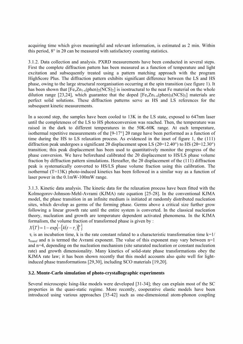
4. RESULTS 4.1. Kinetics of light-induced spin transition in the [FexZn1-x(phen)2(NCS)2] series The powder x-ray diffraction pattern of the neat [Fe(phen)2(NCS)2] and diluted [Fe0.5Zn0.5(phen)2(NCS)2] have been analyzed as described in the methods section above. The powder diffraction pattern at 13K in the ground LS state and the photo-induced metastable HS state are given in figure 1.

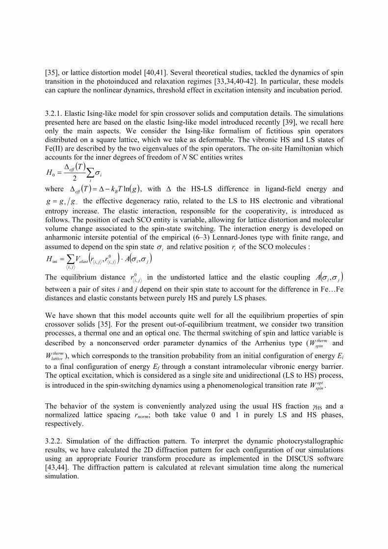
Figure 1. Left : Superposition of 13K LS (in blue) and HS (in red) diffraction patterns for [Fe(phen)2(NCS)2]. Inset: 2θ displacement of the (111) diffraction peak upon LS to HS transition. Right : Low Spin (LS) and photo-induced High Spin (HS) molecular structure of [Fe(phen)2(NCS)2]. The isothermal relaxation curves for the two samples have been followed at various temperatures from 50K to 60K, these are reported in figure 2. All these relaxation curves obviously deviate from a first-order behavior (mono-exponential relaxation), which would have been observed for a purely stochastic molecular relaxation process. Cooperativity plays a key role in the relaxation here. The relaxation curves have been adequately fitted to the rate equation of the KJMA model, which considers a nucleation and domain growth process of phase transformation. In the first stage, the relaxation is quite slow, this corresponds to the incubation time during which germs of the LS phase are formed. In a second step, the relaxation kinetics increases considerably owing to LS domain growth. It is evident that as temperature increases, the incubation time shortens and the relaxation rate increases. This is consistent with a thermally activated process, with easier crossing of the energy barrier as temperature is raised. Interestingly, the relaxation is slower for the diluted sample at each temperature.

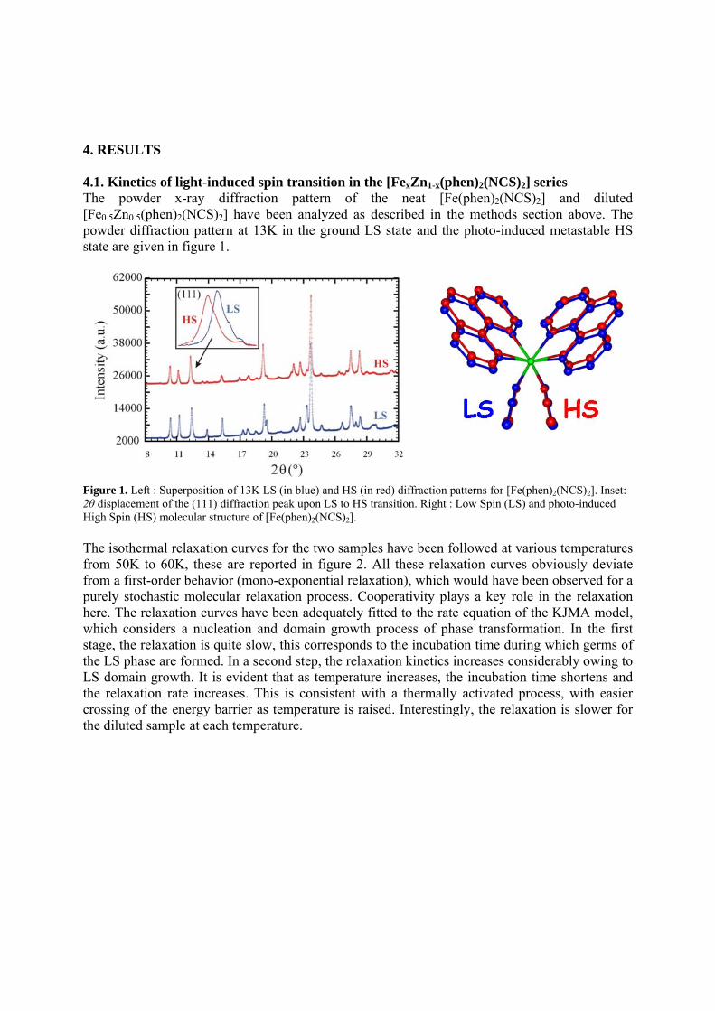
Figure 2. Relaxation kinetics for (a) [Fe(phen)2(NCS)2] and (b) [Fe0.5Zn0.5(phen)2(NCS)2] as a function of temperature from 50K to 60K. Solid lines are least squares fit to the KJMA model. Ln(kHL) as a function of reciprocal temperature is plotted in figure 3. The perfect linear dependence of the Arrhenius plots confirms the validity of a thermally activated process. The activation energy Ea is derived from a linear regression ln(kHL)=A-Ea/kbT, and leads to Ea(x=1.0) = 478 cm-1 and Ea(x=0.5) = 519 cm-1 with frequency factors (pre-exponential factors) of 2.102 s-1 and 2.2.102 s-1 respectively. The present activation energy is directly related to the activation energy to nucleation and domain growth, the relaxation rate kHL(T) in the KJMA formalism is only a function of temperature. We can conclude that the presence of 50% Zn impurity increases the energy barrier to domain growth; these defects probably hinder the propagation of LS domains in the solid. Dilution may enhance the number of favored nucleation sites, however the derived frequency factor is only marginally higher for the doped system. The increased activation energy is not completely compensated by the slightly higher frequency factor, so that globally the relaxation kinetics is slower for the doped [Fe0.5Zn0.5(phen)2(NCS)2] system. In both cases, the fitted Avrami exponent is close to 2.0, which indicates a constant nucleation rate.

Figure 3. Arrhenius plot ln(k) as a function of 1/T for [Fe(phen)2(NCS)2] and [Fe0.5Zn0.5(phen)2(NCS)2].

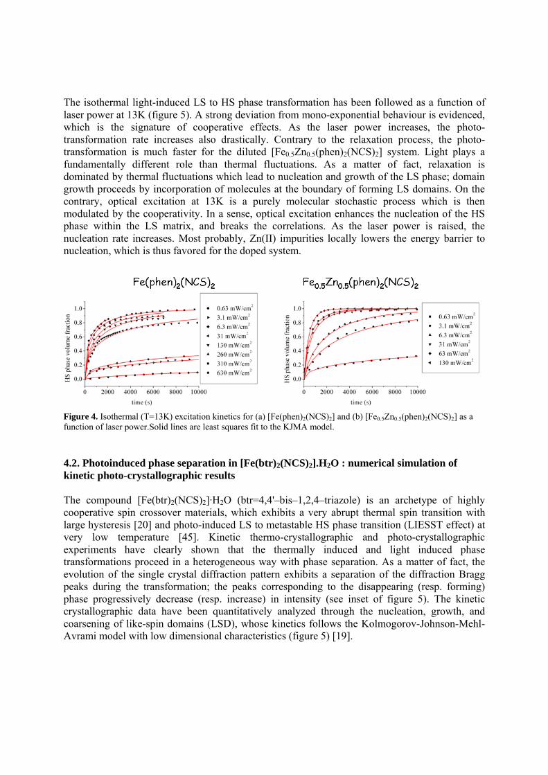
The isothermal light-induced LS to HS phase transformation has been followed as a function of laser power at 13K (figure 5). A strong deviation from mono-exponential behaviour is evidenced, which is the signature of cooperative effects. As the laser power increases, the photo-transformation rate increases also drastically. Contrary to the relaxation process, the photo-transformation is much faster for the diluted [Fe0.5Zn0.5(phen)2(NCS)2] system. Light plays a fundamentally different role than thermal fluctuations. As a matter of fact, relaxation is dominated by thermal fluctuations which lead to nucleation and growth of the LS phase; domain growth proceeds by incorporation of molecules at the boundary of forming LS domains. On the contrary, optical excitation at 13K is a purely molecular stochastic process which is then modulated by the cooperativity. In a sense, optical excitation enhances the nucleation of the HS phase within the LS matrix, and breaks the correlations. As the laser power is raised, the nucleation rate increases. Most probably, Zn(II) impurities locally lowers the energy barrier to nucleation, which is thus favored for the doped system.

Figure 4. Isothermal (T=13K) excitation kinetics for (a) [Fe(phen)2(NCS)2] and (b) [Fe0.5Zn0.5(phen)2(NCS)2] as a function of laser power.Solid lines are least squares fit to the KJMA model. 4.2. Photoinduced phase separation in [Fe(btr)2(NCS)2].H2O : numerical simulation of kinetic photo-crystallographic results The compound [Fe(btr)2(NCS)2]·H2O (btr=4,4'–bis–1,2,4–triazole) is an archetype of highly cooperative spin crossover materials, which exhibits a very abrupt thermal spin transition with large hysteresis [20] and photo-induced LS to metastable HS phase transition (LIESST effect) at very low temperature [45]. Kinetic thermo-crystallographic and photo-crystallographic experiments have clearly shown that the thermally induced and light induced phase transformations proceed in a heterogeneous way with phase separation. As a matter of fact, the evolution of the single crystal diffraction pattern exhibits a separation of the diffraction Bragg peaks during the transformation; the peaks corresponding to the disappearing (resp. forming) phase progressively decrease (resp. increase) in intensity (see inset of figure 5). The kinetic crystallographic data have been quantitatively analyzed through the nucleation, growth, and coarsening of like-spin domains (LSD), whose kinetics follows the Kolmogorov-Johnson-Mehl-Avrami model with low dimensional characteristics (figure 5) [19].

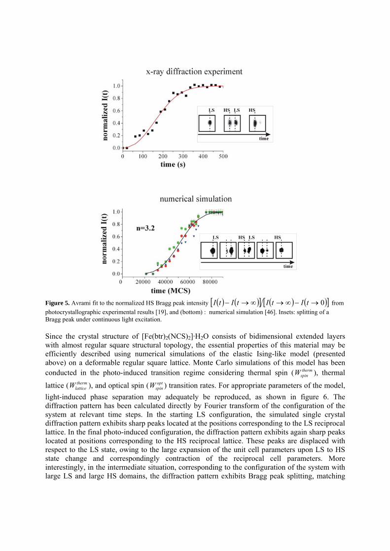
Figure 5. Avrami fit to the normalized HS Bragg peak intensity ( ) ( )[ ] ( ) ( )[ ]0→−∞→∞→− tItItItI from

photocrystallographic experimental results [19], and (bottom) : numerical simulation [46]. Insets: splitting of a Bragg peak under continuous light excitation. Since the crystal structure of [Fe(btr)2(NCS)2]·H2O consists of bidimensional extended layers with almost regular square structural topology, the essential properties of this material may be efficiently described using numerical simulations of the elastic Ising-like model (presented above) on a deformable regular square lattice. Monte Carlo simulations of this model has been conducted in the photo-induced transition regime considering thermal spin ( therm

spinW ), thermal

lattice ( thermlatticeW ), and optical spin ( opt

spinW ) transition rates. For appropriate parameters of the model,

light-induced phase separation may adequately be reproduced, as shown in figure 6. The diffraction pattern has been calculated directly by Fourier transform of the configuration of the system at relevant time steps. In the starting LS configuration, the simulated single crystal diffraction pattern exhibits sharp peaks located at the positions corresponding to the LS reciprocal lattice. In the final photo-induced configuration, the diffraction pattern exhibits again sharp peaks located at positions corresponding to the HS reciprocal lattice. These peaks are displaced with respect to the LS state, owing to the large expansion of the unit cell parameters upon LS to HS state change and correspondingly contraction of the reciprocal cell parameters. More interestingly, in the intermediate situation, corresponding to the configuration of the system with large LS and large HS domains, the diffraction pattern exhibits Bragg peak splitting, matching

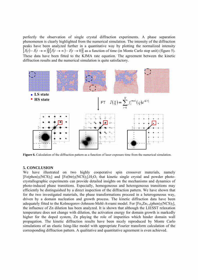
perfectly the observation of single crystal diffraction experiments. A phase separation phenomenon is clearly highlighted from the numerical simulation. The intensity of the diffraction peaks have been analyzed further in a quantitative way by plotting the normalized intensity ( ) ( )[ ] ( ) ( )[ ]0→−∞→∞→− tItItItI as a function of time (in Monte Carlo step unit) (figure 5).

These data have been fitted to the KJMA rate equation. The agreement between the kinetic diffraction results and the numerical simulation is quite satisfactory.

Figure 6. Calculation of the diffraction pattern as a function of laser exposure time from the numerical simulation. 5. CONCLUSION We have illustrated on two highly cooperative spin crossover materials, namely [Fe(phen)2(NCS)2] and [Fe(btr)2(NCS)2].H2O, that kinetic single crystal and powder photo-crystallographic experiments can provide detailed insights on the mechanisms and dynamics of photo-induced phase transitions. Especially, homogeneous and heterogeneous transitions may efficiently be distinguished by a direct inspection of the diffraction pattern. We have shown that for the two investigated materials, the phase transformations proceed in a heterogeneous way, driven by a domain nucleation and growth process. The kinetic diffraction data have been adequately fitted to the Kolmogorov-Johnson-Mehl-Avrami model. For [FexZn1-x(phen)2(NCS)2], the influence of Zn dilution has been analyzed. It is shown that although the LIESST relaxation temperature does not change with dilution, the activation energy for domain growth is markedly higher for the doped system, Zn playing the role of impurities which hinder domain wall propagation. The kinetic diffraction results have been nicely reproduced by Monte Carlo simulations of an elastic Ising-like model with appropriate Fourier transform calculation of the corresponding diffraction pattern. A qualitative and quantitative agreement is even achieved.

ACKNOWLEDGMENTS We thank Jean-François Létard, Philippe Guionneau and Chérif Baldé for providing the [FexZn1-

x(phen)2(NCS)2] series of microcrystalline powder samples. REFERENCES [1] S. Techert and K. A. Zachariasse, J. Am. Chem. Soc. 126 (2004), 5593. [2] P. Coppens, I. Novozhilova, and A. Kovalevsky, Chem. Rev. 102 (2002), 861. [3] P. Coppens, I. I. Vorontsov, T. Graber, M. Gembicky and A. Y. Kovalevsky, Acta Cryst. A61

(2005), 162. [4] E. Collet, M. H. Lemée-Cailleau, M. Buron-Le Cointe, H. Cailleau, M. Wulff, T. Luty, S. Y.

Koshihara, M. Meyer, L. Toupet, P. Rabiller and S. Techert, Science. 300 (2003), 612. [5] T. Friscic and L. R. MacGillivray, Z. Kristallogr. 220 (2005), 351. [6] S. Ohba and Y. Ito, Acta Cryst. B59 (2003), 149. [7] P. Coppens, J. Benedict, M. Messerschmidt, I. Novozhilova, T. Graber, Y.-S. Chen, I. Vorontsov, S. Scheins and S.-L. Zheng, Acta Cryst. A66 (2010), 179. [8] H. Cailleau, M. Lorenc, L. Guérin, M. Servol, E. Collet and M.-L. Buron-Le Cointe, Acta Cryst. A66 (2010), 189. [9] J. B. Benedict, A. Makal, J. D. Sokolow, E. Trzop, S. Scheins, R. Henning, T. Graber and P. Coppens, Chem. Commun. 47 (2011), 1704. [10] M. Chergui, Acta Cryst. A66 (2010), 229. [11] V. Legrand, S. Pillet, H.-P. Weber, M. Souhassou, J.-F. Létard, P. Guionneau and C. Lecomte, J. Appl. Cryst. 40 (2007), 1076. [12] S. Pillet, V. Legrand, H.-P. Weber, M. Souhassou, J.-F. Létard, P. Guionneau and C. Lecomte, Z. Krist. 223 (2008), 235. [13] V. Legrand, S. Pillet, M. Souhassou, N. Lugan and C. Lecomte, J. Am. Chem. Soc. 128 (2006), 13921. [14] Topics in Current Chemistry, Eds. P. Gütlich and H. A. Goodwin (Springer, Berlin, 2004), Vol. 233-235. [15] A. Hauser in : Topics in Current Chemistry, Eds. P. Gütlich and H. A. Goodwin (Springer, Berlin, 2004), Vol. 234, p 155. [16] A. Hauser, Chem. Phys. Lett. 192 (1992), 65. [17] A. Hauser, J. Jeftic, H. Romstedt, R. Hinek and H. Spiering, Coord. Chem. Rev. 190-192 (1999), 471. [18] K. Ichiyanagi, J. Hebert, L. Toupet, H. Cailleau, P. Guionneau, J.-F. Létard, and E. Collet, Phys. Rev. B 73, 060408(R) (2006). [19] S. Pillet, V. Legrand, M. Souhassou, and C. Lecomte, Phys. Rev. B 74, 140101(R) (2006). [20] S. Pillet, J. Hubsch, and C. Lecomte, Eur. Phys. J. B 38, 541 (2004). [21] C. Chong, A. Slimani, F. Varret, K. Boukheddaden, E. Collet, J.-C. Ameline, R. Bronisz and A. Hauser, Chem. Phys. Lett. 504 (2011), 29. [22] C. Chong, H. Mishra, K. Boukheddaden, S. Denise, G. Bouchez, E. Collet, J.-C. Ameline, A. D. Naik, Y. Garcia and F. Varret, J. Phys. Chem. B114 (2010), 1975. [23] C. Baldé, C. Desplanches, A. Wattiaux, P. Guionneau, P. Gütlich and J.-F. Létard, Dalton Trans. (2008), 2702. [24] C. Baldé, C. Desplanches, O. Nguyen and J.-F. Létard, J. Phys.: Conference Series 148 (2009), 012026. [25] A. N. Kolmogorov, Bull. Acad. Sci. URSS (Cl. Sci. Math. Nat.) 3 (1937), 355. [26] W. A. Johnson and R. F. Mehl, Trans. Am. Inst. Min. Engin. 135 (1939), 416.

[27] M. Avrami, J. Chem. Phys. 7 (1939), 1103. [28] M. Avrami, J. Chem. Phys. 8 (1940), 212. [29] M. Bertmer, R. C. Nieuwendaal, A. B. Barnes and S. E. Hayes, J. Phys. Chem. B 110 (2006), 6270. [30] M. Ito, H. Kamioka andY. Moritomo, J. Phys. Soc. Jap. 80 (2011), 023703. [31] A. Bousseksou, H. Constant-Machado and F. Varret, J. Phys. I 5 (1995), 747. [32] K. Boukheddaden, I. Shteto, B. Hôo and F. Varret, Phys. Rev. B 62 (2000), 14796. [33] K. Boukheddaden, I. Shteto, B. Hôo and F. Varret, Phys. Rev. B 62 (2000), 14806. [34] H. Romstedt, A. Hauser and H. Spiering, J. Phys. Chem. Solids 59 (1998), 265. [35] J. A. Nasser, Eur. Phys. J. B 21 (2001), 3. [36] M. Nishino, K. Boukheddaden, Y. Konishi and S. Miyashita, Phys. Rev. Lett. 98 (2007), 247203. [37] M. Nishino, K. Boukheddaden and S. Miyashita, Phys. Rev. B 79 (2009), 012409. [38] Y. Konishi, H. Tokoro, M. Nishino and S. Miyashita, Phys. Rev. Lett. 100 (2008), 067206. [39] W. Nicolazzi, S. Pillet and C. Lecomte, Phys. Rev. B 78 (2008), 174401. [40] O. Sakai, T. Ogawa and K. Koshino, J. Phys. Soc. Jpn. 71 (2002), 978. [41] O. Sakai, M. Ishii, T. Ogawa and K. Koshino, J. Phys. Soc. Jpn. 71 (2002), 2052. [42] T. Kawamoto and S. Abe, Phys. Rev. B 68 (2003), 235112. [43] B. D. Butler and T. R. Welberry, J. Appl. Crystallogr. 25 (1992), 391. [44] T. Proffen and R. B. Neder, J. Appl. Crystallogr. 30 (1997), 171. [45] V. Legrand, S. Pillet, C. Carbonera, M. Souhassou, J.-F. Létard, P. Guionneau and C. Lecomte, Eur. J. Inorg. Chem. 36 (2007), 5693. [46] W. Nicolazzi, S. Pillet and C. Lecomte, Phys. Rev. B 80 (2009), 132102.

Combined Charge Spin and Momentum Densities Refinement : Application to Magnetic Molecular Materials

Claude Lecomtea, Maxime Deutscha, Mohamed Souhassoua, Nicolas Claisera, Sebastien Pilleta,

Pierre Beckerb, Jean-Michel Gilletb, Béatrice Gillonc and Dominique Luneaud

a Laboratoire de Cristallographie, Résonance Magnétique et Modélisations (UMR CNRS 7036), BP 70239,

54506 Vandoeuvre-lès-Nancy France.

b Laboratoire. S.P.M.S., UMR CNRS 8580, École Centrale Paris, Grande Voie des Vignes, 92295 Chatenay-

Malabry France.

c Laboratoire Léon Brillouin (CEA-CNRS, UMR 12), Centre d'Etudes de Saclay, 91191 Gif-sur-Yvette France.

d Laboratoire des Multimatériaux et Interfaces (UMR 5615), Université Claude Bernard Lyon-1, 69622

Villeurbanne Cedex (France)

Introduction Interaction between crystals and X-ray/polarized neutrons, is due to all/unpaired electrons and allow describing and modelling the charge and spin density in position space (Coppens, 1997, Brown et al, 1980) (X-ray / polarized neutron diffraction) and in momentum space (Compton scattering / magnetic Compton scattering) (Cooper et al, 2004). Nowadays, models are mostly derived from one single experiment: X-ray diffraction and charge density modelling, polarized neutron diffraction and spin density modelling... and few attempts have been made to combine several experiments in order to have a more general and thorough electron density modelling. P. Coppens et al (1981) were among the first to propose a joint X-ray/neutron refinement in order to limit the effects of correlation between structural and charge density parameters. This X+N multipolar refinement (Hansen & Coppens 1978) was applied on oxalic acid dehydrate and it was found that the X+N model deformation density shows higher peaks in the lone pair regions. The weighting schemes have been discussed but are not of primary importance in that case because the number of neutron and X-ray diffraction data was similar; it was also shown that the dependence of the x,y,z,Uij structural parameters was in line with their X/N form factors. Schwarzenbach and co-workers (Lewis et al, 1982) have refined the charge density in α Al2O3 with respect to very accurate ultra high resolution data (1.5 Å-1) with AgKα radiation under the constraints of electric field gradient tensors at both Al and O atomic sites, using Hirshfeld deformation functions (Hirshfeld, 1977) and showed that this joint refinement mainly affects the quadrupolar deformation terms as expected. However the very strong anisotropic extinction did not allow drawing more conclusions about the quality of the density. More recently, several papers

report on the possibility to recover the diagonal part of the one particle reduced density matrix (1-RDM for more details see part 5):

( ) 4 41 1 1 2 1 2 2

*N N N; ' N ( , , , ) ( ' , , , )d d= ∫x x x x x x x x x x… … …Γ ψ ψ (1)

from X-ray refinements by minimizing the resulting energy (Jayatilaka & Grimwood, 2001, Grimwood & Jayatilaka, 2001, Bytheway et al., 2002b, Bytheway et al., 2002a, Grimwood et al., 2003) or imposing mathematical constraints like idempotency (Tanaka, 1988, Howard et al, 1994, Massa et al, 1985). All this research has been performed to give a more reliable model of the paired electron density in position space than from X-ray data refinement solely. In the case of magnetic crystals, the description of the electronic structure in position space relies on two diffraction experiments: - X-rays for all electron density - polarized neutrons (PN) for unpaired electron density. Both may be modelled using the Hansen Coppens multipole model (in the polarized neutrons experiment there are no core contributions to the scattering):

maxl l

3 3core val v l lm lm

l 0 m 0

( r ) ( r ) P ( r ) ' R ( ' r ) P y ( , )ρ ρ κ ρ κ κ κ θ φ± ±= =

= + + ∑ ∑

(2)

where ylm are the real spherical harmonics which differ from the corresponding Ylmp by normalizing conditions, R(κ’r ) are Slater type functions, κ and κ’ are expansion contraction coefficients. The net charge of the atom or spin population were estimated from the Pv/Poo parameters obtained respectively from X-ray and PN diffraction data but never from a joint X-ray, PND refinement as proposed by Becker & Coppens (1985). One of the problems to perform such a joint least squares refinement is the unbalanced number of observations as discussed below. According to the Hohenberg-Kohn theorem, if such a joint diffraction approach may yield an exact experimental

density and by consequence, the diagonal part of ( )11 ';xxΓ , the non diagonal parts related to the

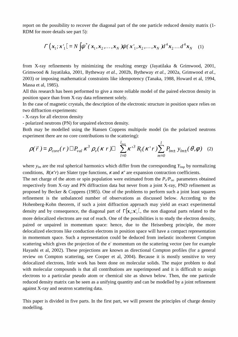
more delocalized electrons are out of reach. One of the possibilities is to study the electron density, paired or unpaired in momentum space: hence, due to the Heisenberg principle, the more delocalized electrons like conduction electrons in position space will have a compact representation in momentum space. Such a representation could be deduced from inelastic incoherent Compton scattering which gives the projection of the e- momentum on the scattering vector (see for example Hayashi et al, 2002). These projections are known as directional Compton profiles (for a general review on Compton scattering, see Cooper et al, 2004). Because it is mostly sensitive to very delocalized electrons, little work has been done on molecular solids. The major problem to deal with molecular compounds is that all contributions are superimposed and it is difficult to assign electrons to a particular pseudo atom or chemical site as shown below. Then, the one particule reduced density matrix can be seen as a unifying quantity and can be modelled by a joint refinement against X-ray and neutron scattering data. This paper is divided in five parts. In the first part, we will present the principles of charge density modelling.

The second part is devoted to spin density measurements. The third part will propose a strategy for a joint X-rays, neutron and polarized neutrons refinement The next part gives preliminary results applied to an end-to-end Azido Double Bridged CuII di nuclear complex (Cu2L2(N3)2) (L=1,1,1-trifluoro-7-(dimethylamino)-4-methyl-5-aza-3-hepten-2-onato). The last part will discuss how to go further in taking into account the non-magnetic and magnetic Compton scattering data. 1 Charge density measurement and modelling

In the kinematic approximation, the intensity of a Bragg reflection is proportional to the square of

the structure factor amplitude, ( )2

oF ; (for more details see, Blessing & Lecomte, 1991)

[ ] 223 **)/( oeoBragg FPLAVvrII λ≈ (3)

with Io the intensity of the incident X-rays beam supposed homogeneous and bathing the whole crystal, λ the wavelength, re the classical electron radius, L the Lorentz correction, P the polarization factor and A is the absorption factor. The measured intensity includes the Bragg reflection along with other contributions for which appropriate and accurate corrections are required:

[ ]1meas Bragg m Bragg m bkgm

I ( ) K I ( ) ( ) y( ) p I ( ) Iα= + + +∑H H H H H (4)

meas 1 m Bragg m bkgm

I ( ) KI ( ) p I ( ) I= + +∑H H H

The background (bkg) includes: Compton scattering, scattering by crystal mount, by air, fluorescence… Multiple scattering should also be corrected for: several reciprocal lattice points Hm may be in reflecting position simultaneously with H , α is the thermal diffuse contribution at the Bragg reflection and y the extinction coefficient:

yLPA

IKF

)1(

' 12

0 α+= (5)

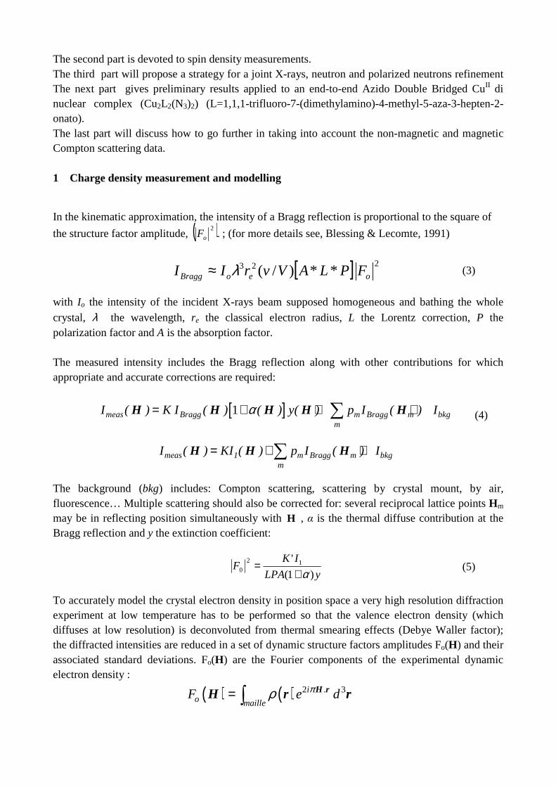
To accurately model the crystal electron density in position space a very high resolution diffraction experiment at low temperature has to be performed so that the valence electron density (which diffuses at low resolution) is deconvoluted from thermal smearing effects (Debye Waller factor); the diffracted intensities are reduced in a set of dynamic structure factors amplitudes Fo(H) and their associated standard deviations. Fo(H) are the Fourier components of the experimental dynamic electron density :

( ) ( ) 2 3i .o maille

F e dπρ= ∫H rH r r

with ( ) ( ) ( )urr Pstat ⊗= ρρ = ∫ − uuur 3)()( dPstatρ .

In the harmonic approximation, for a given atom in the unit cell,

( )

112

3

1

2

j kjk ( u u )

P( ) eσ

π σ

−−=u (6)

Where σ is the determinant ( product of the three eigen values ) by convolution theorem, the dynamic structure factor is:

( ) 2

1

j

Nati .

dyn j jj

F f e T ( )π

== ∑

H rH H (7)

The static structure factor is therefore:

( ) ( ) 2

1

j

Nati .

Stat jj

F f eπ

==∑

H rH H (8)

where fj is the scattering (or form) factor of atom j, Fourier transform of the total atomic electron density:

2 3i .

Vf ( ) ( )e dπρ= ∫

H rH r r (9)

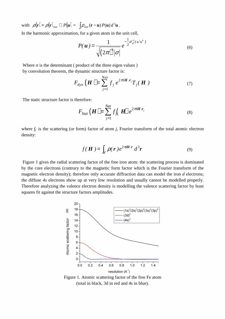
Figure 1 gives the radial scattering factor of the free iron atom: the scattering process is dominated by the core electrons (contrary to the magnetic form factor which is the Fourier transform of the magnetic electron density); therefore only accurate diffraction data can model the iron d electrons; the diffuse 4s electrons show up at very low resolution and usually cannot be modelled properly. Therefore analyzing the valence electron density is modelling the valence scattering factor by least squares fit against the structure factors amplitudes.

Figure 1. Atomic scattering factor of the free Fe atom

(total in black, 3d in red and 4s in blue).

This fit can be performed within the Hansen Coppens formalism (Hansen Coppens, 1978)

∑∑=

±±=

++=l

0mlmlm

l

llvalvcore yPrRPrr

max

),()'(')r()()(0

33 ϕθκκκρκρρ (10)

The corresponding scattering (or form ) factor for any ylm multipole density is

lnlm nl lmf ( ) i f ( H )y ( u,v )=H (11)

where u,v are the angular coordinates of vector H. The refined parameters are the expansion contraction coefficients κ,κ’ and the Pval and Plm populations

This allows computing static deformation maps

l max l

3 3stat val v val v l lm lm

l 0 m 0

( ) P ( r ) N ( r ) ' R ( ' r ) P y ( , )∆ρ κ ρ κ ρ κ κ θ φ± ±= =

= − + ∑ ∑r (12)

The Plm populations , l = 2 and 4, are related to the d orbitals populations through linear equations (Holladay et al, 1983) under the assumption that covalency is negligible; this can be applied to charge and spin density analysis .

2 Spin density measurements In PND experiments, a monochromatic polarized neutron beam with polarization vector P is

diffracted by a magnetically ordered single crystal. The diffracted intensities I+(ΚΚΚΚ) and I-(ΚΚΚΚ) of the

Bragg reflection with scattering vector K =2πH depend on the direction of polarization of the incident beam, parallel or antiparallel to the vertical applied magnetic field:

( ) ( ) 2

N MI ( ) F . ⊥± = ±K K P F K

(13)

where FN and FM refer to nuclear and magnetic structure factors. The magnetic structure factor

( )MF K is a vector, the direction of which is that of the magnetic moment µµµµ resulting from the

sum of the atomic moments µµµµι due to spin and orbit in the unit cell. Its magnitude is related to the normalized magnetization density m(r) by Fourier transform:

( ) ( ) i

cell

m e d= ∫Kr

MF K µ r r (14)

( )⊥MF K is its component perpendicular to the scattering vector: ( ) ( )ˆ ˆ⊥ = × ×M MF K K F K K , where

K is a unit vector parallel to the scattering vector ΚΚΚΚ, as shown in Figure 2.

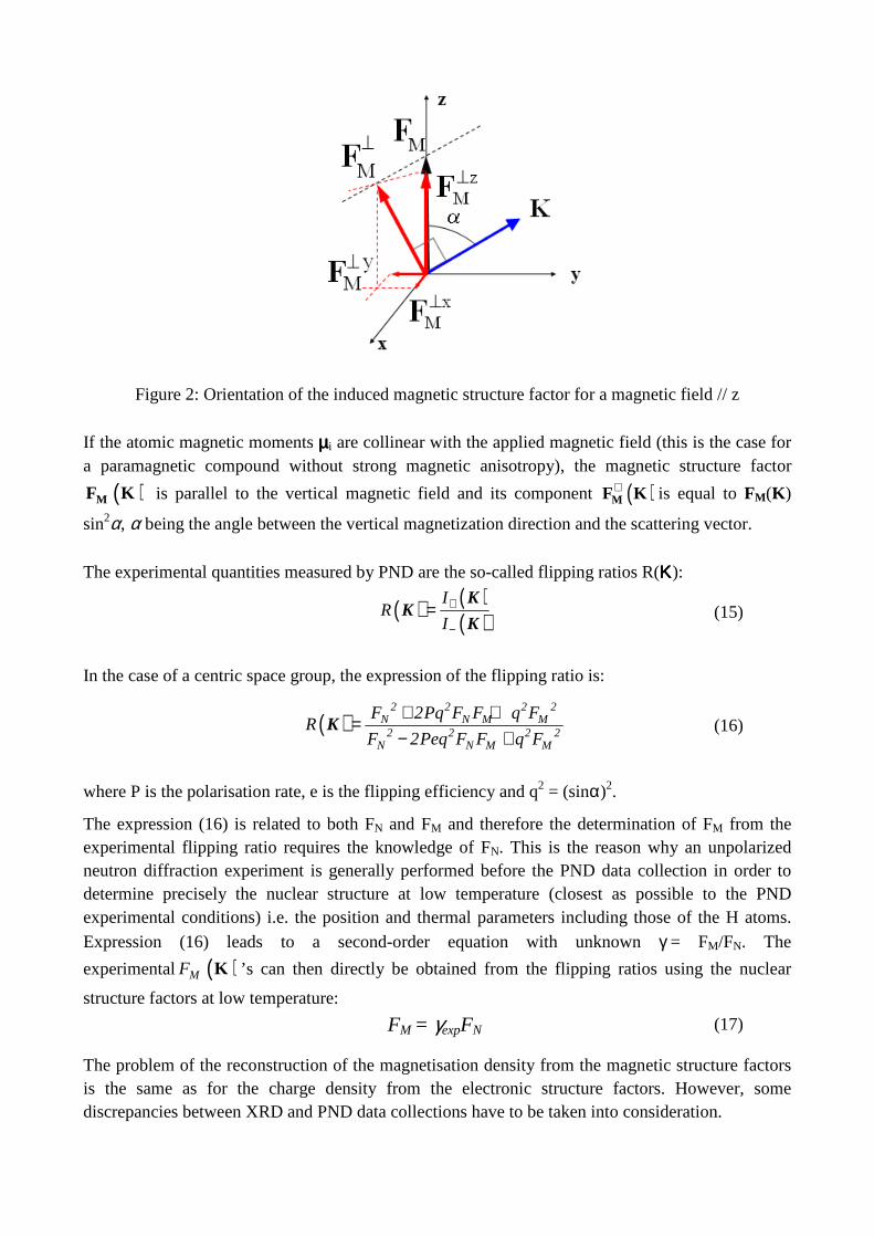
Figure 2: Orientation of the induced magnetic structure factor for a magnetic field // z

If the atomic magnetic moments µµµµi are collinear with the applied magnetic field (this is the case for a paramagnetic compound without strong magnetic anisotropy), the magnetic structure factor

( )MF K is parallel to the vertical magnetic field and its component ( )⊥MF K is equal to FM(K)

sin2α, α being the angle between the vertical magnetization direction and the scattering vector. The experimental quantities measured by PND are the so-called flipping ratios R(ΚΚΚΚ):

( ) ( )( )

IR

I+

−=

KK

K (15)

In the case of a centric space group, the expression of the flipping ratio is:

( )2 2 2 2

N N M M2 2 2 2

N N M M

F 2Pq F F q FR

F 2Peq F F q F

+ +=− +

K (16)

where P is the polarisation rate, e is the flipping efficiency and q2 = (sinα)2.

The expression (16) is related to both FN and FM and therefore the determination of FM from the experimental flipping ratio requires the knowledge of FN. This is the reason why an unpolarized neutron diffraction experiment is generally performed before the PND data collection in order to determine precisely the nuclear structure at low temperature (closest as possible to the PND experimental conditions) i.e. the position and thermal parameters including those of the H atoms. Expression (16) leads to a second-order equation with unknown γ = FM/FN. The

experimental ( )MF K ’s can then directly be obtained from the flipping ratios using the nuclear

structure factors at low temperature:

FM = γexpFN (17)

The problem of the reconstruction of the magnetisation density from the magnetic structure factors is the same as for the charge density from the electronic structure factors. However, some discrepancies between XRD and PND data collections have to be taken into consideration.

First of all, the number of observations in PND data collections is generally smaller than in XRD data collections, especially for molecular compounds. A first reason is that form factors of 2p and 3d shells decrease more rapidly than total electronic form factors for light atoms and transition metals as it can be seen in Figure 1. That is why the PND data collections are generally limited to smaller (sinθ/λ)max than XRD. For recall, in the independent atoms model, the magnetic structure factors are written as a discrete sum over the atoms in the cell:

( ) ( )a

i i

ni Wi

i magi 1

F e e−

== ∑ κR

MF κ µ κ (18)

where ( )κimagF is the normalized magnetic form factor of atom i, carrying a magnetic moment µµµµi and

Wi is the Debye-Waller factor of this atom:

( ) ( )i imag iF m e d= ∫

κrκ r r (19)

In the spherical approximation, the magnetic form factor is the Fourier transform of the unpaired electron radial density mi(r) centered on atom i and is analogous to the radial scattering factor displayed for 3d electrons in Figure 1. In addition, for weakly magnetic materials, only the magnetic structure factor corresponding to strong or medium nuclear structure factors can be accessed because of the relation (17). Therefore important magnetic structure factors may be missing in the data collection. On another hand, PND is generally applied to ferro, ferri or paramagnetic compounds in which a large enough magnetization can be induced by a magnetic field, at the difference to antiferromagnetic materials.

Secondly, because the experimental quantity R is a ratio between two intensities, it is not affected by absorption effects nor by scale factor. Therefore the value of the magnetisation in the cell can be directly deduced from the determination of the spin density. In the joint refinement method, we shall constrain the sum of the spin populations over the atoms of the molecular unit to be equal to the number of unpaired electrons. Therefore the scale factor refined for PND in this work provides a value of the magnetisation in the conditions of field and temperature during the data collection.

When studying molecular materials which usually contain a large number of hydrogen atoms, additional terms have to be introduced in the expression (16) of the flipping ratio, accounting for the contribution due to the polarization of the hydrogen nuclear spins at very low temperature and high magnetic field, with a polarization factor given by:

i 4NP

H(Tesla)f 14.89.10

T(K)−= (10-12 cm) (20)

The general expression of the flipping ratio taking into account this last contribution is:

2 2 2 2 2

N N M NP M NP M NP2 2 2 2 2

N N M NP M NP M NP

F 2PF ( q F F ) q F F 2qF FR( )

F 2PeF ( q F F ) q F F 2qF F

+ + + + +=− + + + +

K (21)

where FNP is the structure factor due to H nuclear polarisation and FM is the experimental magnetic structure factor due to spin and orbit.

For transition metal with non zero angular momentum, the orbital contribution has to be taken into account in order to retrieve the pure spin contribution. For that purpose the dipole approximation [Squires 1978] is used to evaluate the magnetic form factor due to angular momentum:

( )LM s 0 2

( g 2 )F ( ) j j

gµ −= +K (22)

where µs is the pure spin moment and g is the Landé factor.

3 Joint X-ray and polarized neutron refinement: Methodology and strategy

In this chapter we discuss the strategy for a joint refinement of the spin and charge densities according to an extended Hansen Coppens model which distinguishes the up and down spin contributions. The charge density is thus described as

r r

max max

3 3core

l ll l3 3

l lm lm l lm lml 0 m 0 l 0 m 0

( ) ( r ) P ( ) P ( )

' R ( ' r ) P y ( , ) ' R ( ' r ) P y ( , )

ν ν ν νρ ρ κ ρ κ κ ρ κ

κ κ θ φ κ κ θ φ

↑ ↑ ↑ ↑ ↓ ↓ ↓ ↓

↑ ↑ ↑ ↓ ↓ ↓± ± ± ±

= = = =

= + + +

+∑ ∑ ∑ ∑

r

(23)

↑νP and ↓

νP are the valence population of the electrons with spin up and down respectively,

associated with their respective ↑κ / ↓κ . ±↑

lmP and ±↓

lmP are multipole populations corresponding to spin up and down. The spin up and spin down electron distributions may not have the same radial

extension and that is taken into account by ↑κ / ↓κ and ↑'κ / ↓'κ . Therefore the refinement (up and down parameters) against X-ray and PND data lead to a simultaneous determination of spin and charge density and to the corresponding density maps. For atoms carrying a magnetic moment, the spin density is the difference between spin up and spin down densities:

3 3

3 3

0 0

r r

max maxl ll l

l lm lm l lm lml m 0 l m 0

s( ) P ( ) P ( )

' R ( ' r ) P y ( , ) ' R ( ' r ) P y ( , )

ν ν ν νκ ρ κ κ ρ κ

κ κ θ φ κ κ θ φ

↑ ↑ ↑ ↑ ↓ ↓ ↓ ↓

↑ ↑ ↑ ↓ ↓ ↓± ± ± ±

= = = =

= − +

−∑ ∑ ∑ ∑

r

(24)

To carry out such a refinement gathering X-ray, unpolarized neutrons (UPN) and polarized neutrons (PND) data, we make the following assumptions: - The cell parameters are those obtained from the X-ray experiments. - Two sets of anisotropic atomic displacement parameters Uij and extinction parameters are refined from X-ray and neutron separately. - The electroneutrality (all X-rays monopoles) and total magnetic moment (spin monopoles) constraints are added using Hamilton method (Hamilton, 1965). One of the main concerns in the joint refinement strategy is the weighting scheme: because we deal with a complete X-rays data set to very high or high resolution compared to medium resolution and incomplete PN data set, the weights have to be carefully assigned.

The easiest model is to use a score function C that minimises the sum of the χ2 of each experiment which should favour the large data sets; this model was used in the joint refinement (neutrons and X-ray) by Coppens and co-workers (Coppens et al,1981):

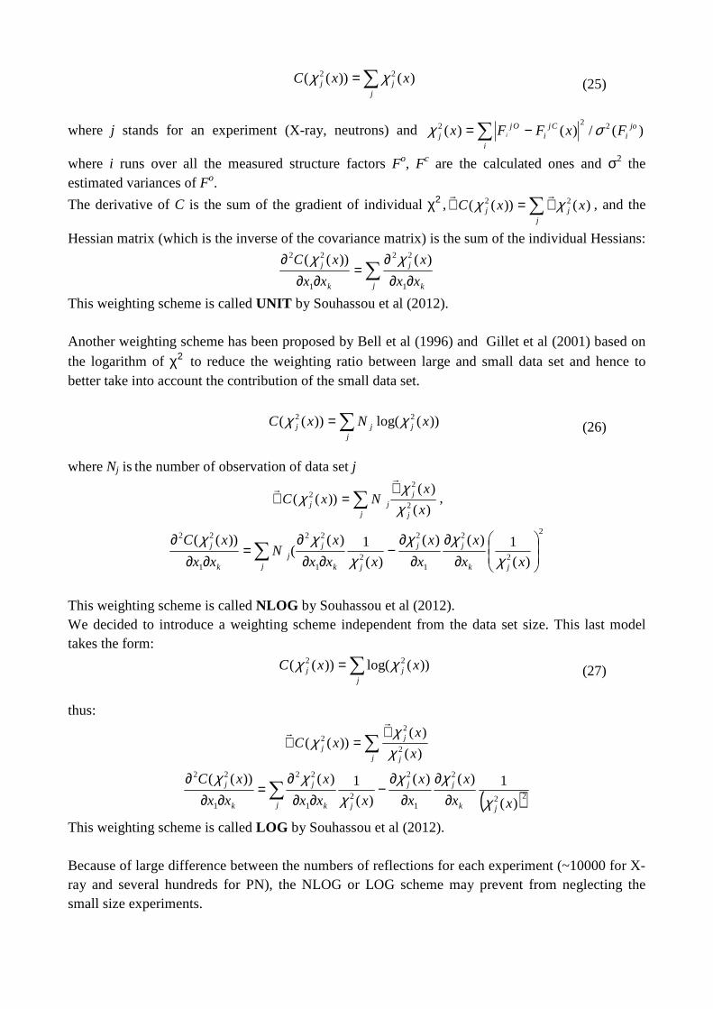
)())(( 22 xxCj

jj ∑= χχ (25)

where j stands for an experiment (X-ray, neutrons) and )(/)()( 222 ∑ −=i

joi

Cji

Ojj FxFFx i σχ

where i runs over all the measured structure factors Fo, Fc are the calculated ones and σ2 the estimated variances of Fo.

The derivative of C is the sum of the gradient of individual χ2 , )())(( 22 xxCj

jj ∑∇=∇ χχ

, and the

Hessian matrix (which is the inverse of the covariance matrix) is the sum of the individual Hessians:

∑ ∂∂∂

=∂∂

∂

j k

j

k

j

xx

x

xx

xC

1

22

1

22 )())(( χχ

This weighting scheme is called UNIT by Souhassou et al (2012). Another weighting scheme has been proposed by Bell et al (1996) and Gillet et al (2001) based on

the logarithm of χ2 to reduce the weighting ratio between large and small data set and hence to better take into account the contribution of the small data set.

))(log())(( 22 xNxCj

jjj ∑= χχ (26)

where Nj is the number of observation of data set j

∑∇

=∇j j

jjj x

xNxC

)(

)())((

2

22

χχ

χ

,

2

2

2

1

2

21

22

1

22

)(

1)()(

)(

1)((

))((

∂∂

∂∂

−∂∂

∂=

∂∂∂

∑xx

x

x

x

xxx

xN

xx

xC

jk

jj

jj k

jj

k

j

χχχ

χχχ

This weighting scheme is called NLOG by Souhassou et al (2012). We decided to introduce a weighting scheme independent from the data set size. This last model takes the form:

))(log())(( 22 xxCj

jj ∑= χχ (27)

thus:

∑∇

=∇j j

jj x

xxC

)(

)())((

2

22

χχ

χ

( )22

2

1

2

21

22

1

22

)(

1)()(

)(

1)())((

xx

x

x

x

xxx

x

xx

xC

jk

jj

jj k

j

k

j

χ

χχχ

χχ∂

∂∂

∂−

∂∂∂

=∂∂

∂∑

This weighting scheme is called LOG by Souhassou et al (2012). Because of large difference between the numbers of reflections for each experiment (~10000 for X-ray and several hundreds for PN), the NLOG or LOG scheme may prevent from neglecting the small size experiments.

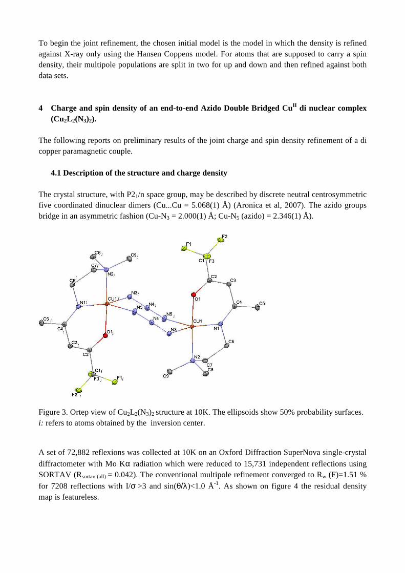
To begin the joint refinement, the chosen initial model is the model in which the density is refined against X-ray only using the Hansen Coppens model. For atoms that are supposed to carry a spin density, their multipole populations are split in two for up and down and then refined against both data sets. 4 Charge and spin density of an end-to-end Azido Double Bridged CuII di nuclear complex

(Cu2L2(N3)2). The following reports on preliminary results of the joint charge and spin density refinement of a di copper paramagnetic couple.

4.1 Description of the structure and charge density

The crystal structure, with P21/n space group, may be described by discrete neutral centrosymmetric five coordinated dinuclear dimers (Cu...Cu = 5.068(1) Å) (Aronica et al, 2007). The azido groups bridge in an asymmetric fashion (Cu-N3 = 2.000(1) Å; Cu-N5 (azido) = 2.346(1) Å).

Figure 3. Ortep view of Cu2L2(N3)2 structure at 10K. The ellipsoids show 50% probability surfaces. i: refers to atoms obtained by the inversion center. A set of 72,882 reflexions was collected at 10K on an Oxford Diffraction SuperNova single-crystal

diffractometer with Mo Kα radiation which were reduced to 15,731 independent reflections using SORTAV (Rsortav (all) = 0.042). The conventional multipole refinement converged to Rw (F)=1.51 %

for 7208 reflections with I/σ >3 and sin(θ/λ)<1.0 Å-1. As shown on figure 4 the residual density map is featureless.

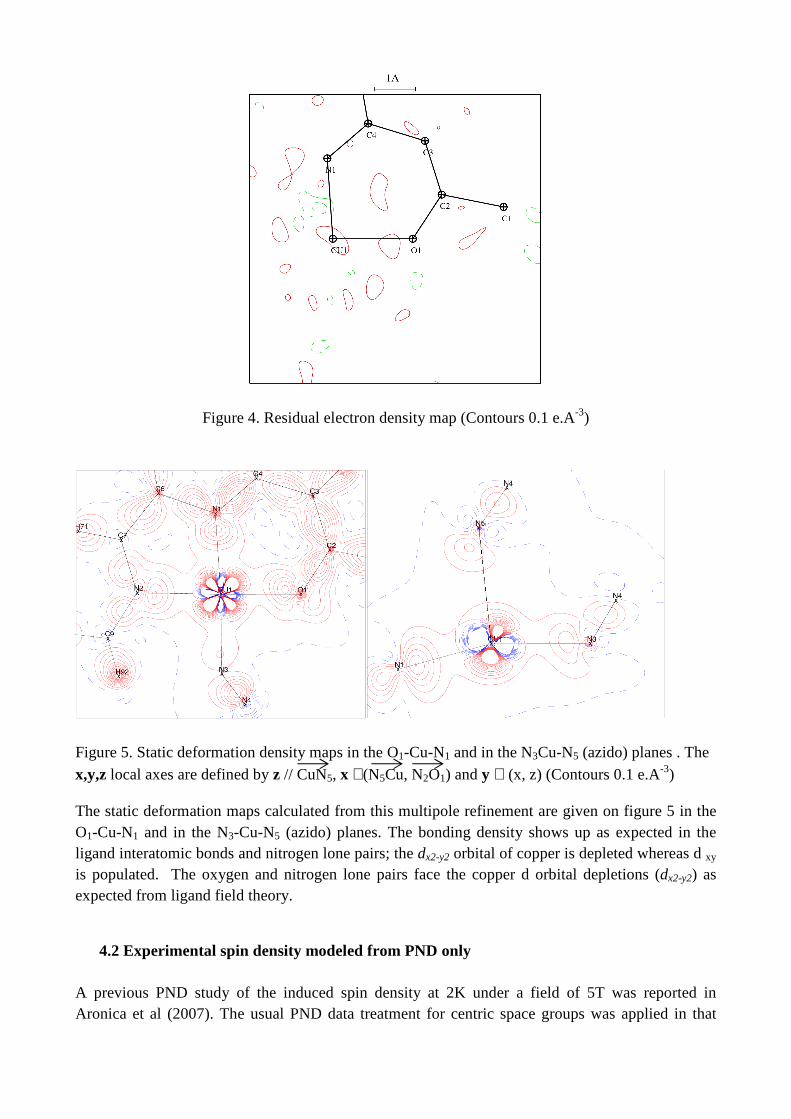
Figure 4. Residual electron density map (Contours 0.1 e.A-3)

Figure 5. Static deformation density maps in the O1-Cu-N1 and in the N3Cu-N5 (azido) planes . The

x,y,z local axes are defined by z // CuN5, x ⊥(N5Cu, N2O1) and y ⊥ (x, z) (Contours 0.1 e.A-3) The static deformation maps calculated from this multipole refinement are given on figure 5 in the O1-Cu-N1 and in the N3-Cu-N5 (azido) planes. The bonding density shows up as expected in the ligand interatomic bonds and nitrogen lone pairs; the dx2-y2 orbital of copper is depleted whereas d xy is populated. The oxygen and nitrogen lone pairs face the copper d orbital depletions (dx2-y2) as expected from ligand field theory.

4.2 Experimental spin density modeled from PND only A previous PND study of the induced spin density at 2K under a field of 5T was reported in Aronica et al (2007). The usual PND data treatment for centric space groups was applied in that

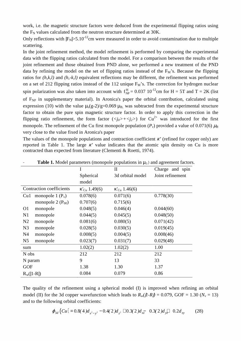
work, i.e. the magnetic structure factors were deduced from the experimental flipping ratios using the FN values calculated from the neutron structure determined at 30K.

Only reflections with |FN|>5.10-12cm were measured in order to avoid contamination due to multiple scattering. In the joint refinement method, the model refinement is performed by comparing the experimental data with the flipping ratios calculated from the model. For a comparison between the results of the joint refinement and those obtained from PND alone, we performed a new treatment of the PND data by refining the model on the set of flipping ratios instead of the FM’s. Because the flipping ratios for (h,k,l) and (h,-k,l) equivalent reflections may be different, the refinement was performed on a set of 212 flipping ratios instead of the 112 unique FM’s. The correction for hydrogen nuclear

spin polarization was also taken into account with HNPf = 0.037 10-12cm for H = 5T and T = 2K (list

of FNP in supplementary material). In Aronica's paper the orbital contribution, calculated using

expression (10) with the value µs(g-2)/g=0.069 µB, was subtracted from the experimental structure factor to obtain the pure spin magnetic structure factor. In order to apply this correction in the flipping ratio refinement, the form factor (<j 0>+<j 2>) for Cu2+ was introduced for the first

monopole. The refinement of the Cu first monopole population (Pv) provided a value of 0.071(6) µB very close to the value fixed in Aronica's paper

The values of the monopole populations and contraction coefficient κ’ (refined for copper only) are reported in Table 1. The large κ’ value indicates that the atomic spin density on Cu is more contracted than expected from literature (Clementi & Roetti, 1974). - Table 1. Model parameters (monopole populations in µB)and agreement factors.

I Spherical model

II 3d orbital model

Charge and spin Joint refinement

Contraction coefficients κ'Cu 1.49(6) κ'Cu 1.46(6)

Cu1 monopole 1 (Pv) 0.078(6) 0.071(6) 0.778(30) monopole 2 (P00) 0.707(6) 0.715(6) O1 monopole 0.048(5) 0.046(4) 0.044(60) N1 monopole 0.044(5) 0.045(5) 0.048(50) N2 monopole 0.081(6) 0.080(5) 0.071(42) N3 monopole 0.028(5) 0.030(5) 0.019(45) N4 monopole 0.008(5) 0.004(5) 0.008(46) N5 monopole 0.023(7) 0.031(7) 0.029(48) sum 1.02(2) 1.02(2) 1.00 N obs 212 212 212 N param 9 13 33 GOF 1.38 1.30 1.37

Rw(|1-R|) 0.084 0.079 0.86

The quality of the refinement using a spherical model (I) is improved when refining an orbital

model (II) for the 3d copper wavefunction which leads to Rw(|1-R|) = 0.079, GOF = 1.30 (Nv = 13) and to the following orbital coefficients:

( ) 2 2 23 0 8 4 0 4 2 0 3 2 0 3 2 0 2d xz yz xyx y zCu . ( )d . ( )d . ( )d . ( )d . dϕ −= − + − + (28)

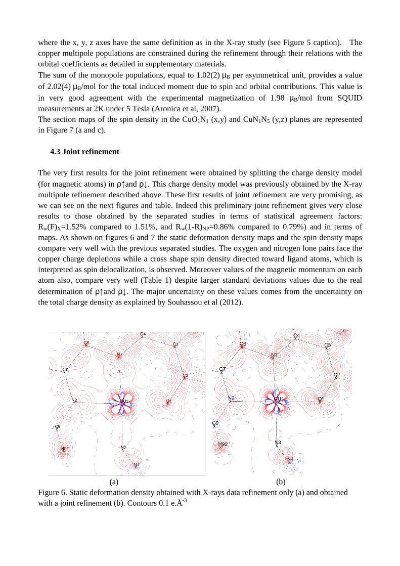
where the x, y, z axes have the same definition as in the X-ray study (see Figure 5 caption). The copper multipole populations are constrained during the refinement through their relations with the orbital coefficients as detailed in supplementary materials. The sum of the monopole populations, equal to 1.02(2) µB per asymmetrical unit, provides a value

of 2.02(4) µB/mol for the total induced moment due to spin and orbital contributions. This value is

in very good agreement with the experimental magnetization of 1.98 µB/mol from SQUID measurements at 2K under 5 Tesla (Aronica et al, 2007). The section maps of the spin density in the CuO1N1 (x,y) and CuN1N5 (y,z) planes are represented in Figure 7 (a and c).

4.3 Joint refinement

The very first results for the joint refinement were obtained by splitting the charge density model

(for magnetic atoms) in ρ↑and ρ↓. This charge density model was previously obtained by the X-ray multipole refinement described above. These first results of joint refinement are very promising, as we can see on the next figures and table. Indeed this preliminary joint refinement gives very close results to those obtained by the separated studies in terms of statistical agreement factors: Rw(F)X=1.52% compared to 1.51%, and Rw(1-R)NP=0.86% compared to 0.79%) and in terms of maps. As shown on figures 6 and 7 the static deformation density maps and the spin density maps compare very well with the previous separated studies. The oxygen and nitrogen lone pairs face the copper charge depletions while a cross shape spin density directed toward ligand atoms, which is interpreted as spin delocalization, is observed. Moreover values of the magnetic momentum on each atom also, compare very well (Table 1) despite larger standard deviations values due to the real

determination of ρ↑and ρ↓. The major uncertainty on these values comes from the uncertainty on the total charge density as explained by Souhassou et al (2012).

(a) (b) Figure 6. Static deformation density obtained with X-rays data refinement only (a) and obtained with a joint refinement (b). Contours 0.1 e.Å-3

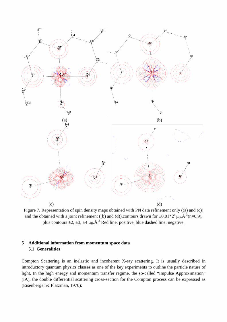
(a) (b)

(c) (d) Figure 7. Representation of spin density maps obtained with PN data refinement only ((a) and (c)) and the obtained with a joint refinement ((b) and (d)).contours drawn for ±0.01*2n

µB.Å-3(n=0,9), plus contours ±2, ±3, ±4 µB.Å-3 Red line: positive, blue dashed line: negative.

5 Additional information from momentum space data

5.1 Generalities Compton Scattering is an inelastic and incoherent X-ray scattering. It is usually described in introductory quantum physics classes as one of the key experiments to outline the particle nature of light. In the high energy and momentum transfer regime, the so-called “Impulse Approximation” (IA), the double differential scattering cross-section for the Compton process can be expressed as (Eisenberger & Platzman, 1970):

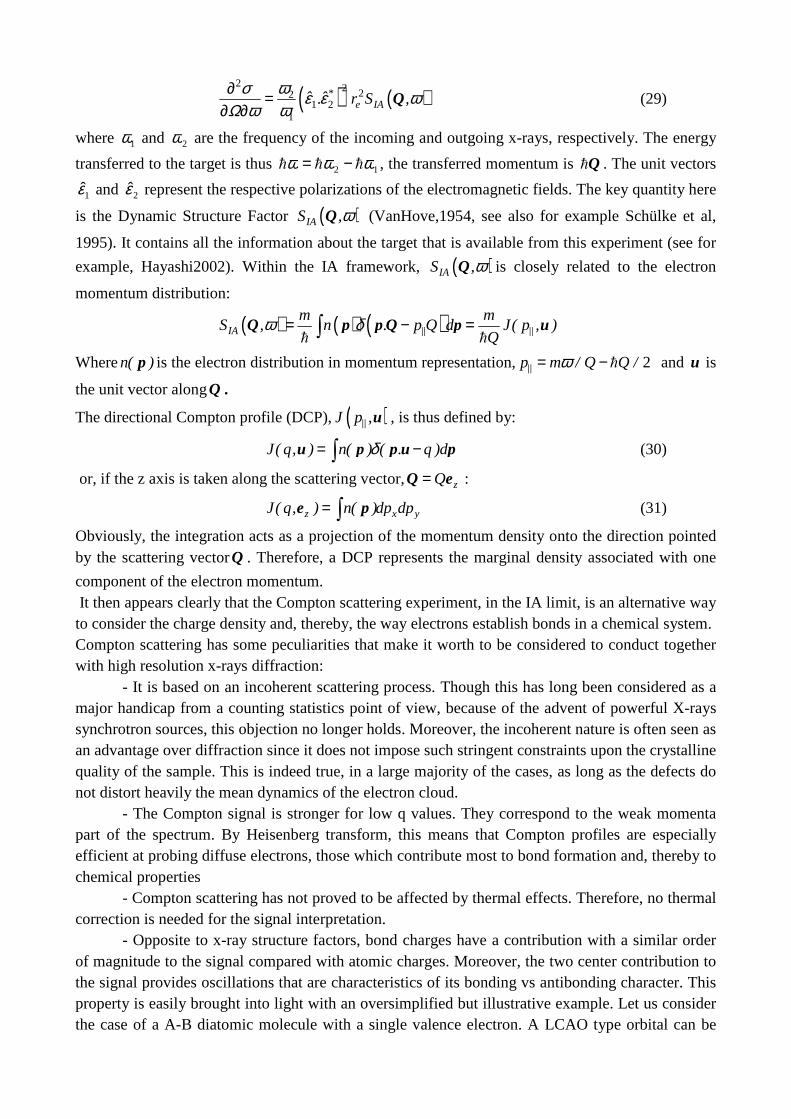
( ) ( )2 2 22

1 21

*e IAˆ ˆ. r S ,

ωσ ε ε ωΩ ω ω∂ =

∂ ∂Q (29)

where 1ω and 2ω are the frequency of the incoming and outgoing x-rays, respectively. The energy

transferred to the target is thus 12 ωωω ℏℏℏ −= , the transferred momentum is Qℏ . The unit vectors

1ε and 2ε represent the respective polarizations of the electromagnetic fields. The key quantity here

is the Dynamic Structure Factor ( )IAS ,ωQ (VanHove,1954, see also for example Schülke et al,

1995). It contains all the information about the target that is available from this experiment (see for

example, Hayashi2002). Within the IA framework, ( )IAS ,ωQ is closely related to the electron

momentum distribution:

( ) ( ) ( )IAm m

S , n . p Q d J( p , )Q

ω δ= − =∫Q p p Q p u ℏ ℏ

Wheren( )p is the electron distribution in momentum representation, 2p m / Q Q /ω= − ℏ and u is

the unit vector alongQ .

The directional Compton profile (DCP),( )J p ,u , is thus defined by:

J( q, ) n( ) ( . q )dδ= −∫u p p u p (30)

or, if the z axis is taken along the scattering vector, zQ=Q e :

z x yJ( q, ) n( )dp dp= ∫e p (31)

Obviously, the integration acts as a projection of the momentum density onto the direction pointed by the scattering vectorQ . Therefore, a DCP represents the marginal density associated with one

component of the electron momentum. It then appears clearly that the Compton scattering experiment, in the IA limit, is an alternative way to consider the charge density and, thereby, the way electrons establish bonds in a chemical system. Compton scattering has some peculiarities that make it worth to be considered to conduct together with high resolution x-rays diffraction:

- It is based on an incoherent scattering process. Though this has long been considered as a major handicap from a counting statistics point of view, because of the advent of powerful X-rays synchrotron sources, this objection no longer holds. Moreover, the incoherent nature is often seen as an advantage over diffraction since it does not impose such stringent constraints upon the crystalline quality of the sample. This is indeed true, in a large majority of the cases, as long as the defects do not distort heavily the mean dynamics of the electron cloud.

- The Compton signal is stronger for low q values. They correspond to the weak momenta part of the spectrum. By Heisenberg transform, this means that Compton profiles are especially efficient at probing diffuse electrons, those which contribute most to bond formation and, thereby to chemical properties

- Compton scattering has not proved to be affected by thermal effects. Therefore, no thermal correction is needed for the signal interpretation.

- Opposite to x-ray structure factors, bond charges have a contribution with a similar order of magnitude to the signal compared with atomic charges. Moreover, the two center contribution to the signal provides oscillations that are characteristics of its bonding vs antibonding character. This property is easily brought into light with an oversimplified but illustrative example. Let us consider the case of a A-B diatomic molecule with a single valence electron. A LCAO type orbital can be

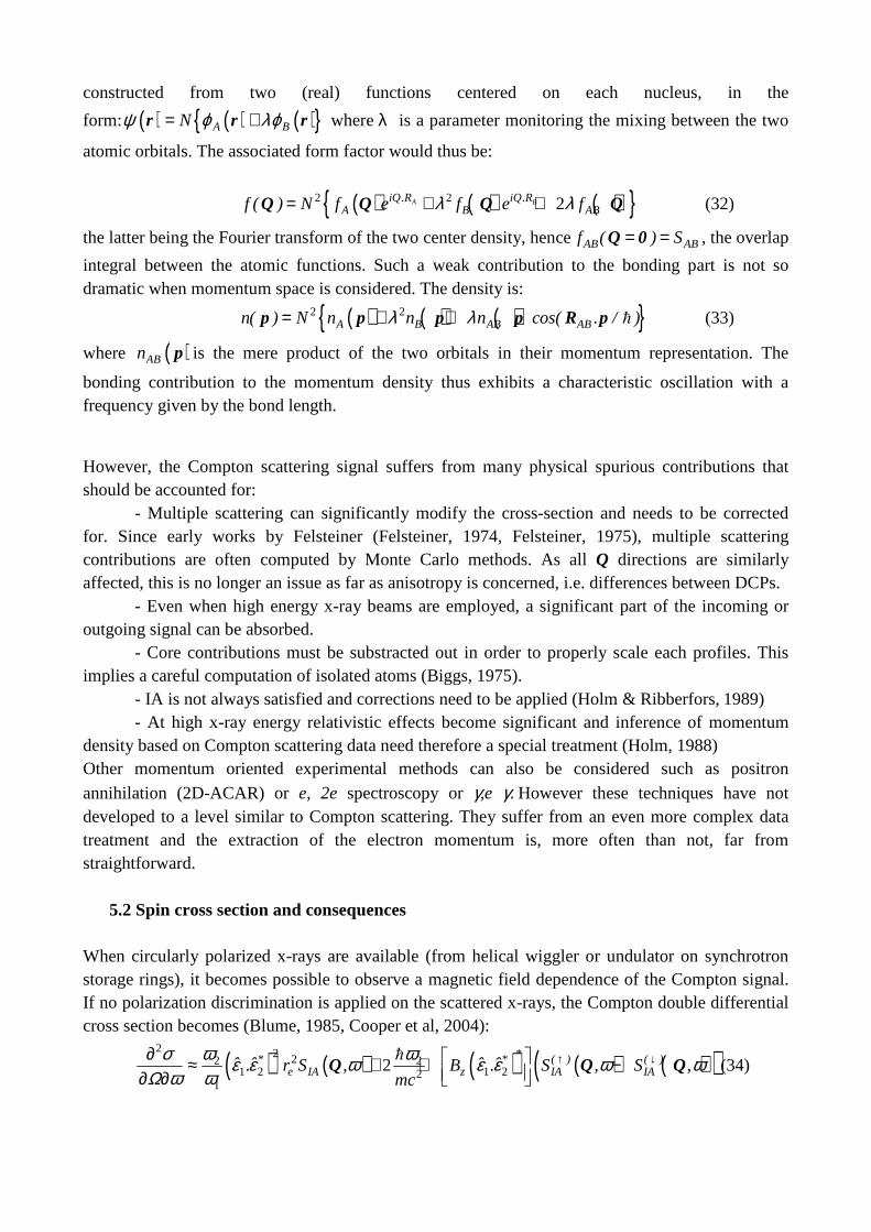
constructed from two (real) functions centered on each nucleus, in the

form: ( ) ( ) ( ) A BNψ ϕ λϕ= +r r r where λ is a parameter monitoring the mixing between the two

atomic orbitals. The associated form factor would thus be:

( ) ( ) ( ) 2 2 2A BiQ.R iQ.RA B ABf ( ) N f e f e fλ λ= + +Q Q Q Q (32)

the latter being the Fourier transform of the two center density, henceAB ABf ( ) S= =Q 0 , the overlap

integral between the atomic functions. Such a weak contribution to the bonding part is not so dramatic when momentum space is considered. The density is:

( ) ( ) ( ) 2 2A B AB ABn( ) N n n n cos( . / )λ λ= + +p p p p R p ℏ (33)

where ( )ABn p is the mere product of the two orbitals in their momentum representation. The

bonding contribution to the momentum density thus exhibits a characteristic oscillation with a frequency given by the bond length.

However, the Compton scattering signal suffers from many physical spurious contributions that should be accounted for:

- Multiple scattering can significantly modify the cross-section and needs to be corrected for. Since early works by Felsteiner (Felsteiner, 1974, Felsteiner, 1975), multiple scattering contributions are often computed by Monte Carlo methods. As all Q directions are similarly affected, this is no longer an issue as far as anisotropy is concerned, i.e. differences between DCPs.

- Even when high energy x-ray beams are employed, a significant part of the incoming or outgoing signal can be absorbed.

- Core contributions must be substracted out in order to properly scale each profiles. This implies a careful computation of isolated atoms (Biggs, 1975).

- IA is not always satisfied and corrections need to be applied (Holm & Ribberfors, 1989) - At high x-ray energy relativistic effects become significant and inference of momentum

density based on Compton scattering data need therefore a special treatment (Holm, 1988) Other momentum oriented experimental methods can also be considered such as positron annihilation (2D-ACAR) or e, 2e spectroscopy or γ,e γ. However these techniques have not developed to a level similar to Compton scattering. They suffer from an even more complex data treatment and the extraction of the electron momentum is, more often than not, far from straightforward.

5.2 Spin cross section and consequences When circularly polarized x-rays are available (from helical wiggler or undulator on synchrotron storage rings), it becomes possible to observe a magnetic field dependence of the Compton signal. If no polarization discrimination is applied on the scattered x-rays, the Compton double differential cross section becomes (Blume, 1985, Cooper et al, 2004):

( ) ( ) ( ) ( ) ( )( )2 2 22 2

1 2 1 221

2** * ( ) ( )

e IA z IA IAˆ ˆ ˆ ˆ. r S , B . S , S ,mc

ω ωσ ε ε ω ε ε ω ωΩ ω ω

↑ ↓∂ ≈ + ℑ − ∂ ∂ Q Q Q

ℏ(34)

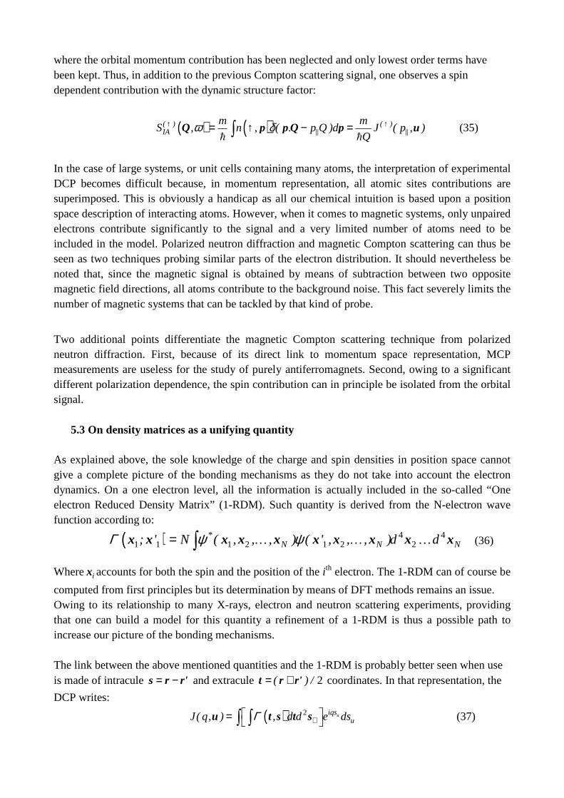
where the orbital momentum contribution has been neglected and only lowest order terms have been kept. Thus, in addition to the previous Compton scattering signal, one observes a spin dependent contribution with the dynamic structure factor:

( ) ( )( ) ( )IA

m mS , n , ( . p Q )d J ( p , )

Qω δ↑ ↑= ↑ − =∫Q p p Q p u

ℏ ℏ (35)

In the case of large systems, or unit cells containing many atoms, the interpretation of experimental DCP becomes difficult because, in momentum representation, all atomic sites contributions are superimposed. This is obviously a handicap as all our chemical intuition is based upon a position space description of interacting atoms. However, when it comes to magnetic systems, only unpaired electrons contribute significantly to the signal and a very limited number of atoms need to be included in the model. Polarized neutron diffraction and magnetic Compton scattering can thus be seen as two techniques probing similar parts of the electron distribution. It should nevertheless be noted that, since the magnetic signal is obtained by means of subtraction between two opposite magnetic field directions, all atoms contribute to the background noise. This fact severely limits the number of magnetic systems that can be tackled by that kind of probe.

Two additional points differentiate the magnetic Compton scattering technique from polarized neutron diffraction. First, because of its direct link to momentum space representation, MCP measurements are useless for the study of purely antiferromagnets. Second, owing to a significant different polarization dependence, the spin contribution can in principle be isolated from the orbital signal.

5.3 On density matrices as a unifying quantity

As explained above, the sole knowledge of the charge and spin densities in position space cannot give a complete picture of the bonding mechanisms as they do not take into account the electron dynamics. On a one electron level, all the information is actually included in the so-called “One electron Reduced Density Matrix” (1-RDM). Such quantity is derived from the N-electron wave function according to:

( ) 4 41 1 1 2 1 2 2

*N N N; ' N ( , , , ) ( ' , , , )d d= ∫x x x x x x x x x x… … …Γ ψ ψ (36)

Where ix accounts for both the spin and the position of the i th electron. The 1-RDM can of course be

computed from first principles but its determination by means of DFT methods remains an issue. Owing to its relationship to many X-rays, electron and neutron scattering experiments, providing that one can build a model for this quantity a refinement of a 1-RDM is thus a possible path to increase our picture of the bonding mechanisms. The link between the above mentioned quantities and the 1-RDM is probably better seen when use is made of intracule = −s r r' and extracule 2( ) /= +t r r' coordinates. In that representation, the

DCP writes:

( ) 2 uiqsuJ( q, ) , d d e dsΓ ⊥ = ∫ ∫u t s t s (37)

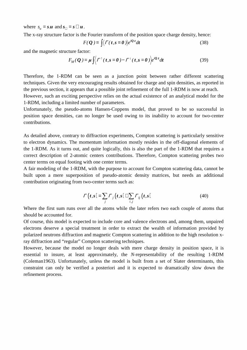
where us .= s u and ⊥ = ⊗s s u.

The x-ray structure factor is the Fourier transform of the position space charge density, hence: i .F( ) ( , ) e dΓ= =∫Q tQ t s 0 t (38)

and the magnetic structure factor: i .

MF ( ) ( , ) ( , ) e dΓ Γ↑ ↓= = − =∫Q tQ µ t s 0 t s 0 t (39)

Therefore, the 1-RDM can be seen as a junction point between rather different scattering techniques. Given the very encouraging results obtained for charge and spin densities, as reported in the previous section, it appears that a possible joint refinement of the full 1-RDM is now at reach. However, such an exciting perspective relies on the actual existence of an analytical model for the 1-RDM, including a limited number of parameters. Unfortunately, the pseudo-atoms Hansen-Coppens model, that proved to be so successful in position space densities, can no longer be used owing to its inability to account for two-center contributions. As detailed above, contrary to diffraction experiments, Compton scattering is particularly sensitive to electron dynamics. The momentum information mostly resides in the off-diagonal elements of the 1-RDM. As it turns out, and quite logically, this is also the part of the 1-RDM that requires a correct description of 2-atomic centers contributions. Therefore, Compton scattering probes two center terms on equal footing with one center terms. A fair modeling of the 1-RDM, with the purpose to account for Compton scattering data, cannot be built upon a mere superposition of pseudo-atomic density matrices, but needs an additional contribution originating from two-center terms such as:

( ) ( ) ( )j ijj i , j

, , ,Γ Γ Γ= +∑ ∑t s t s t s (40)

Where the first sum runs over all the atoms while the later refers two each couple of atoms that should be accounted for. Of course, this model is expected to include core and valence electrons and, among them, unpaired electrons deserve a special treatment in order to extract the wealth of information provided by polarized neutrons diffraction and magnetic Compton scattering in addition to the high resolution x-ray diffraction and “regular” Compton scattering techniques. However, because the model no longer deals with mere charge density in position space, it is essential to insure, at least approximately, the N-representability of the resulting 1-RDM (Coleman1963). Unfortunately, unless the model is built from a set of Slater determinants, this constraint can only be verified a posteriori and it is expected to dramatically slow down the refinement process.

Acknowledgement: .

This work has been supported by l'Agence Nationale de la Recherche (CEDA Project) and M.D. thanks

C.N.R.S for PhD fellowship

References Aronica, C., Jeanneau, E., El Moll, H., Luneau, D., Gillon, B., Goujon, A., Cousson, A., Carvajal, M. A., & Robert, V. (2007). Chem. Eur. J. 13, 3666–3674 Aronica C., Chumakov Y., Jeanneau, E., Luneau D., Neugebauer P., Barra A.L., Gillon B., Goujon

A., Cousson A., Tercero J., Ruiz E., (2008) Chem. Eur. J. 14, 9540 – 9548

Becker, P. & Coppens, P. (1985). Acta Cryst. A 41, 177–182. Bell, B., Burke, J., & Schumitzky, A. (1996). Comp. Stat. And Data Anal 22, 119–135 Biggs F., Mendelsohn L.B., Mann J.B. (1975) Atomic Data and Nuclear Data Tables 16, 201-309 Blume M., J. (1985) Appl. Phys. 57, 3615 . Brown, P. J., Forsyth, J. B., & Mason, R. (1980). Phil. Trans. R. Soc. Lond. B 290, 481–495. Bytheway, I., Grimwood, D., Figgis, B., Chandler, G., & Jayatilaka, D. (2002a). Acta Cryst. A 58, 244–251 Bytheway, I., Grimwood, D., & Jayatilaka, D. (2002b). Acta Cryst. A 58, 232–243. Blessing R.H. and Lecomte C. (1991) in "The application of charge density research to chemistry and drug design", NATO Adv. Studies, G.A. Geffrey and J.F. Piniella eds, 90-120. Clementi, E. & Roetti, C. (1974). Atomic Data and Nuclear Data Tables 14, 177–478. Coleman A.J.(1963) Review of Modern Physics 35, 668-687 Cooper, M. J., Mijnarends, P. E., Shiotani, N., Sakai, N., & Bansil, A. (2004). X-ray Compton scattering. Oxford University Press. Coppens, P., Boehme, R., Price, P. F., & Stevens, E. D. (1981). Acta Cryst. A 37, 857–863. Coppens P. & Becker P. (1992) Analysis of charge and spin densities. Int. Tables for X-ray Crystallography, Vol.C, 627-245. Coppens, P. (1997). X-Ray Charge Densities and Chemical Bonding (International Union of Crystallography Texts on Crystallography , No 4). Oxford University Press.

Eisenberger P. & Platzman P.M.(1970) Compton Scattering of X Rays from Bound Electrons. Phys. Rev. A 2, 415-423, Felsteiner J. & Pattison P., (1975) Nuclear Instruments and Methods, 124, 449-453 Felsteiner J. & Pattison P., Cooper M., (1974) Philosophical Magazine 30, 537-548 Gillet, J.-M., Becker, P. J., & Cortona, P. (2001). Phys. Rev. B 63, 235115 Grimwood, D., Bytheway, I., & Jayatilaka, D. (2003). J. Comput. Chem. 24, 470–483. Grimwood, D. & Jayatilaka, D. (2001). Acta Cryst. A 57, 87–100. Hamilton, W. C. (1965). Acta Cryst. 18, 502–510 Hansen, N. K. & Coppens, P. (1978). Acta Cryst. A 34, 909–921. Hayashi, H., Udagawa, Y., Gillet, J.-M., Caliebe, W., & Kao, C.-C. (2002). Chemical Applications of Synchrotron Radiation volume 12 of Advanced Series in Physical Chemistry chapter 18. World Scientific publishing, Singapore. Hirshfeld F.L. (1977) Isr. J. Chem. 16, 226-229. Holladay, A., Leung, P., & Coppens, P. (1983). Acta Cryst. A 39, 377–387. Holm P. & Ribberfors R. (1989) Phys. Rev. A 40, 6251 Holm P. (1988) Phys. Rev. A 37, 3706 Howard, S., Huke, J., Mallinson, P., & Frampton, C. (1994). Phys. Rev. B 49, 7124–7136. Jayatilaka, D. & Grimwood, D. J. (2001). Acta Cryst. A 57, 76–86. Lewis, J., Schwarzenbach, D., & Flack, H. (1982). Acta Cryst. A 38, 733–739. Massa, L., Goldberg, M., Frishberg, C., Boehme, R., & Placa, S. (1985). Phys. Rev. Lett., 55, 622–625. Sakai N.& Ôno K.(1976) Phys. Rev. Lett.37, 351-353 Schülke W., Schmitz J.R., Schulte-Schrepping H. & Kaprolat A. (1995) Phys. Rev. B 52, 11721-11732, Souhassou M., Deutsch M., Claiser N., Pillet S., Lecomte C., Ciumakov Y., Gillon B. and Gillet J-M (2012) Acta Cryst A in preparation.

Squires G. L. (1978), in Introduction to the Theory of Thermal Neutron Scattering, University Press, Cambridge, p.139 Tanaka, K. (1988). Acta Cryst. A, 44, 1002–1008.

Van Hove L. (1954) Phys. Rev. 95, 249-262,

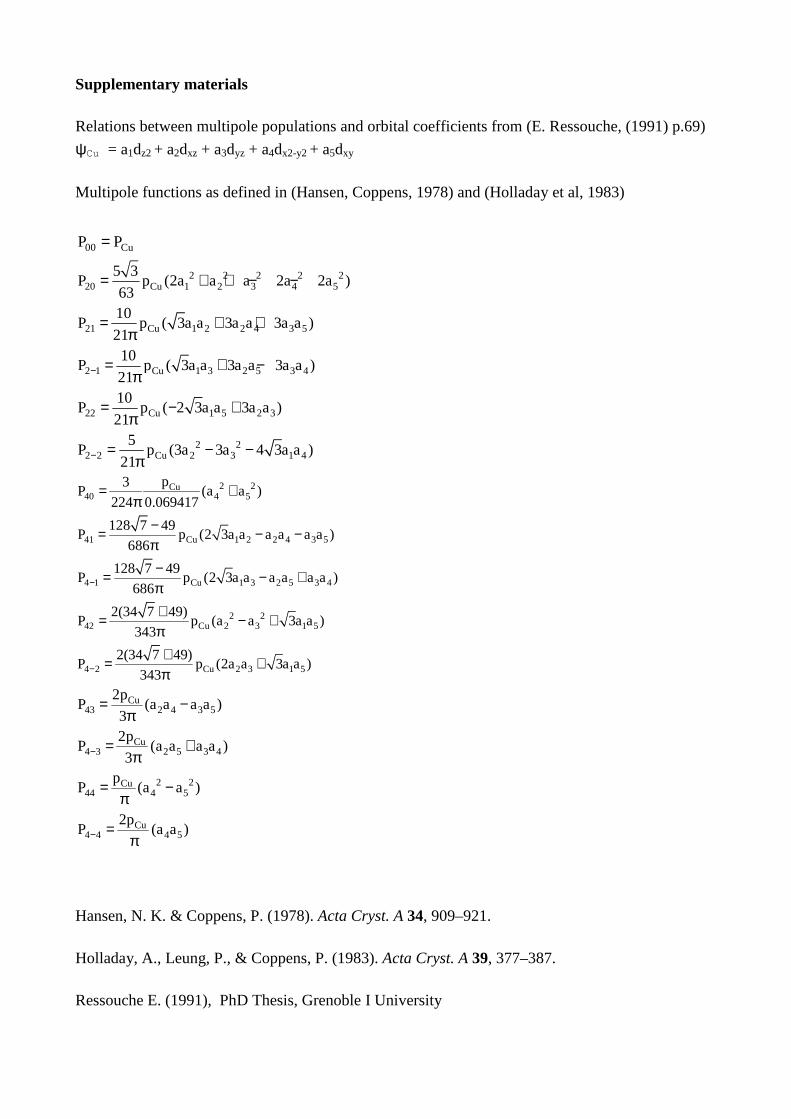
Supplementary materials

Relations between multipole populations and orbital coefficients from (E. Ressouche, (1991) p.69)

ψCu = a1dz2 + a2dxz + a3dyz + a4dx2-y2 + a5dxy

Multipole functions as defined in (Hansen, Coppens, 1978) and (Holladay et al, 1983)

00 CuP P=

2 2 2 2 220 Cu 1 2 3 4 5

5 3P p (2a a a 2a 2a )

63= + + − −

21 Cu 1 2 2 4 3 510

P p ( 3a a 3a a 3a a )21

= + +π

2 1 Cu 1 3 2 5 3 4

10P p ( 3a a 3a a 3a a )

21− = + −π

22 Cu 1 5 2 3

10P p ( 2 3a a 3a a )

21= − +

π 2 2

2 2 Cu 2 3 1 45

P p (3a 3a 4 3a a )21− = − −

π 2 2Cu

40 4 5p3

P (a a )224 0.069417

= +π

41 Cu 1 2 2 4 3 5

128 7 49P p (2 3a a a a a a )

686

−= − −π

4 1 Cu 1 3 2 5 3 4

128 7 49P p (2 3a a a a a a )

686−−= − +π

2 2

42 Cu 2 3 1 52(34 7 49)

P p (a a 3a a )343

+= − +π

4 2 Cu 2 3 1 5

2(34 7 49)P p (2a a 3a a )

343−+= +π

Cu43 2 4 3 5

2pP (a a a a )

3= −

π Cu

4 3 2 5 3 42p

P (a a a a )3− = +π

2 2Cu44 4 5

pP (a a )= −

π

Cu4 4 4 5

2pP (a a )− =

π

Hansen, N. K. & Coppens, P. (1978). Acta Cryst. A 34, 909–921. Holladay, A., Leung, P., & Coppens, P. (1983). Acta Cryst. A 39, 377–387. Ressouche E. (1991), PhD Thesis, Grenoble I University

Distributed atomic polarizabilities from electron density. 1. Motivations and Theory

Anna Krawczuk-Pantula,a Daniel Pérez, a Katarzyna Stadnicka,b Piero Macchi a,*

a) Department of Chemistry and Biochemistry, University of Bern, Freiestrasse 3, 3012 Bern, Switzerland

b) Faculty of Chemistry, Jagiellonian University, Ingardena 3, 30-060 Krakow, Poland

piero.macchi@dcb.unibe.ch

Abstract

In this paper, the distributed atomic polarizabilities computed within the Quantum

Theory of Atoms in Molecules are discussed. Methods are presented to calculate and

visualize symmetric atomic polarizability tensors, with proved additivity to molecular

polarizabilities. The analysis of QTAIM bond polarizabilities is also presented for

some simple molecules and potential applications in material science are anticipated.

Introduction

The response of electron density to an electric field is fundamental to understand,

among the others, the behavior of molecules in chemical reactions, the solvation

properties, the recognition processes and spectroscopic properties. As a matter of

facts, the (hyper)polarizabilities tensors determine the soft ("orbital controlled")

assembly and reactivity of molecules, the intensities of Raman scattering and many

other optical processes. For this reason, measuring or calculating the molecular

(hyper)polarizabilities is of fundamental importance, especially when dealing with

material science. If the material is a crystalline solid, the properties are regulated by

the electric susceptibilities, which are related, for molecular based materials, to the

molecular (hyper)polarizabilities tensors through lattice summation.

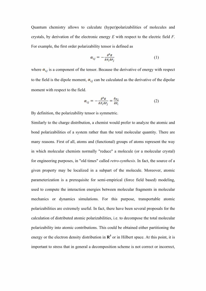
Quantum chemistry allows to calculate (hyper)polarizabilities of molecules and

crystals, by derivation of the electronic energy E with respect to the electric field F.

For example, the first order polarizability tensor is defined as

(1)

where is a component of the tensor. Because the derivative of energy with respect

to the field is the dipole moment, can be calculated as the derivative of the dipolar

moment with respect to the field.

(2)

By definition, the polarizability tensor is symmetric.

Similarly to the charge distribution, a chemist would prefer to analyze the atomic and

bond polarizabilities of a system rather than the total molecular quantity. There are

many reasons. First of all, atoms and (functional) groups of atoms represent the way

in which molecular chemists normally "reduce" a molecule (or a molecular crystal)

for engineering purposes, in "old times" called retro-synthesis. In fact, the source of a

given property may be localized in a subpart of the molecule. Moreover, atomic

parameterization is a prerequisite for semi-empirical (force field based) modeling,

used to compute the interaction energies between molecular fragments in molecular

mechanics or dynamics simulations. For this purpose, transportable atomic

polarizabilities are extremely useful. In fact, there have been several proposals for the

calculation of distributed atomic polarizabilities, i.e. to decompose the total molecular

polarizability into atomic contributions. This could be obtained either partitioning the

energy or the electron density distribution in R3 or in Hilbert space. At this point, it is

important to stress that in general a decomposition scheme is not correct or incorrect,

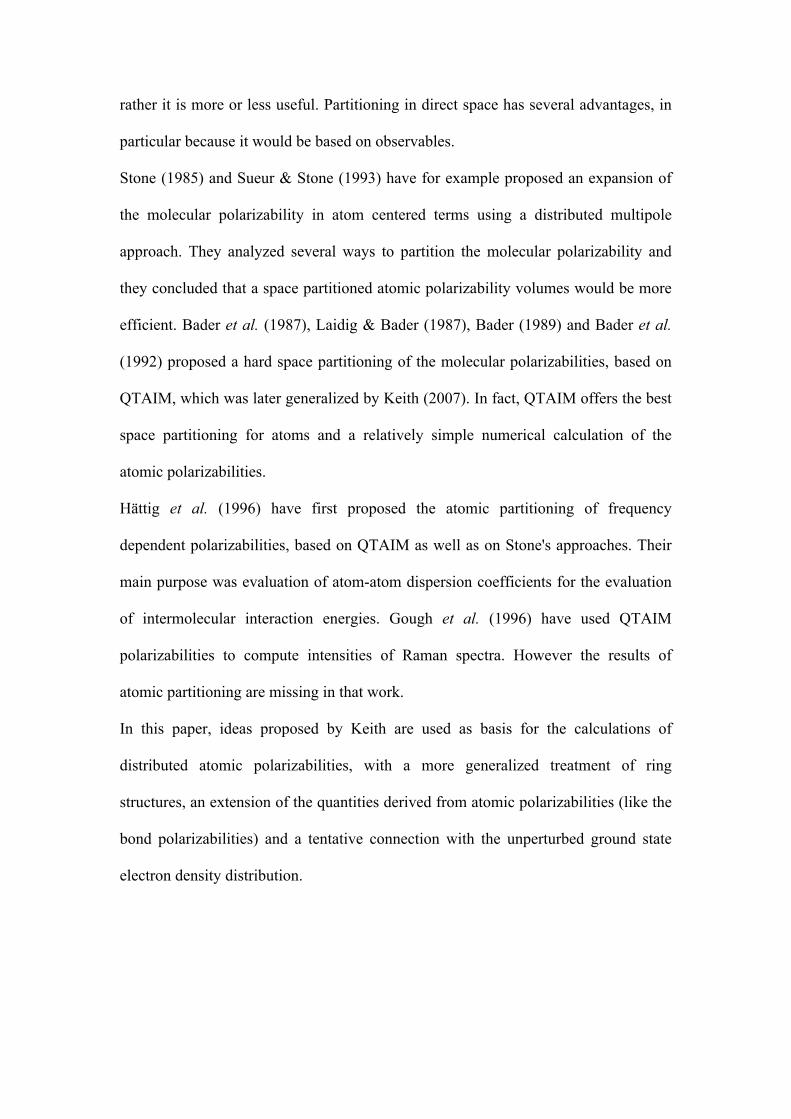
rather it is more or less useful. Partitioning in direct space has several advantages, in

particular because it would be based on observables.

Stone (1985) and Sueur & Stone (1993) have for example proposed an expansion of

the molecular polarizability in atom centered terms using a distributed multipole

approach. They analyzed several ways to partition the molecular polarizability and

they concluded that a space partitioned atomic polarizability volumes would be more

efficient. Bader et al. (1987), Laidig & Bader (1987), Bader (1989) and Bader et al.

(1992) proposed a hard space partitioning of the molecular polarizabilities, based on

QTAIM, which was later generalized by Keith (2007). In fact, QTAIM offers the best

space partitioning for atoms and a relatively simple numerical calculation of the

atomic polarizabilities.

Hättig et al. (1996) have first proposed the atomic partitioning of frequency

dependent polarizabilities, based on QTAIM as well as on Stone's approaches. Their

main purpose was evaluation of atom-atom dispersion coefficients for the evaluation

of intermolecular interaction energies. Gough et al. (1996) have used QTAIM

polarizabilities to compute intensities of Raman spectra. However the results of

atomic partitioning are missing in that work.

In this paper, ideas proposed by Keith are used as basis for the calculations of

distributed atomic polarizabilities, with a more generalized treatment of ring

structures, an extension of the quantities derived from atomic polarizabilities (like the

bond polarizabilities) and a tentative connection with the unperturbed ground state

electron density distribution.

Motivations

The motivations of our work are multifaceted. We are interested in computing,

visualizing and analyzing atomic polarizabilities of some typical functional groups,

providing an advanced tool to "standard" QTAIM analysis, including the possibility

to define the bond polarizability. We also want to extract atomic polarizabilities using

fuzzy partitioning schemes, like Hirshfeld stockholder atoms, to evaluate the more

reliable and useful method. Moreover, we are interested in relating the ground state

unperturbed electron density with the distributed atomic polarizabilities, in the

attempt to estimate semi-empirical atomic and molecular polarizabilities from

experimentally observable electron density distributions.

In a long term view, we expect to use transferable or semi-empirical atomic

polarizabilities to estimate molecular and crystal properties, especially optical

properties, and we are interested in visualizing the polarizability densities, as a tool to

analyze chemical reactivity.

In this initial paper, we report on QTAIM distributed polarizabilities as a complement

of normal QTAIM analysis, providing visualization tools for the atomic

polarizabilities. The paper is structured as it follows: first we discuss the theoretical

background and the partitioning scheme adopted, then we illustrate examples on some

popular molecules, we discuss the results in terms of chemical and finally we

anticipate further work.

Partitioning schemes

Among the possible partitioning scheme, we have focused on the spatial partitioning

of the electron density, in keeping with the Quantum Theory of Atoms in Molecules

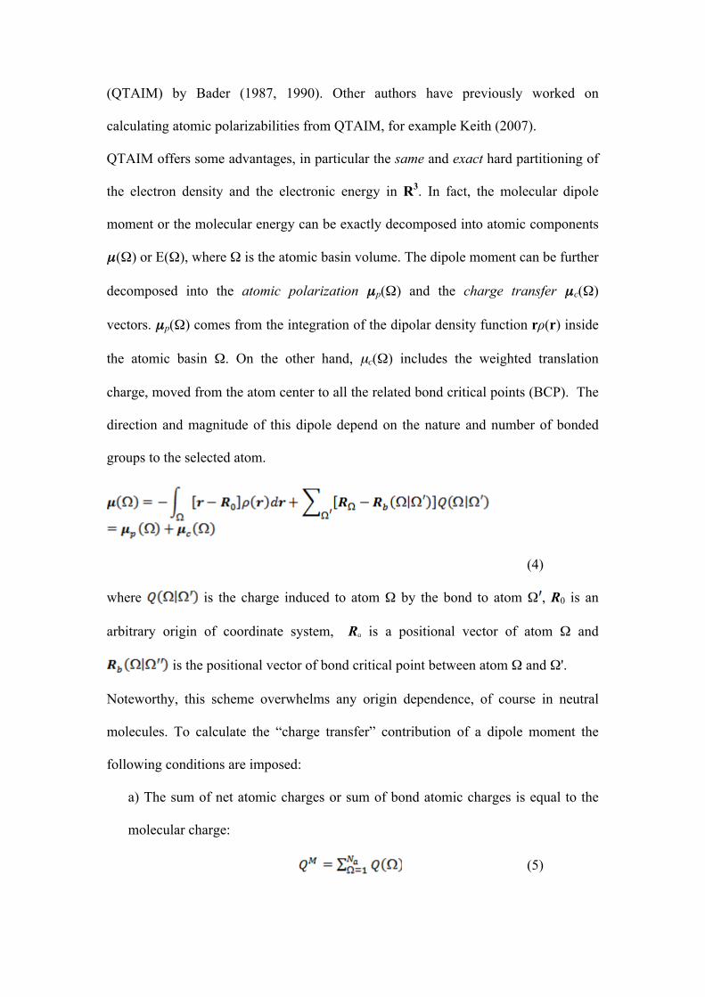
(QTAIM) by Bader (1987, 1990). Other authors have previously worked on

calculating atomic polarizabilities from QTAIM, for example Keith (2007).

QTAIM offers some advantages, in particular the same and exact hard partitioning of

the electron density and the electronic energy in R3. In fact, the molecular dipole

moment or the molecular energy can be exactly decomposed into atomic components

µ(Ω) or E(Ω), where Ω is the atomic basin volume. The dipole moment can be further

decomposed into the atomic polarization µp(Ω) and the charge transfer µc(Ω)

vectors. µp(Ω) comes from the integration of the dipolar density function rρ(r) inside

the atomic basin Ω. On the other hand, µc(Ω) includes the weighted translation

charge, moved from the atom center to all the related bond critical points (BCP). The

direction and magnitude of this dipole depend on the nature and number of bonded

groups to the selected atom.

(4)

where is the charge induced to atom Ω by the bond to atom Ω , R0 is an

arbitrary origin of coordinate system, RΩ is a positional vector of atom Ω and

is the positional vector of bond critical point between atom Ω and Ω'.

Noteworthy, this scheme overwhelms any origin dependence, of course in neutral

molecules. To calculate the “charge transfer” contribution of a dipole moment the

following conditions are imposed:

a) The sum of net atomic charges or sum of bond atomic charges is equal to the

molecular charge:

(5)

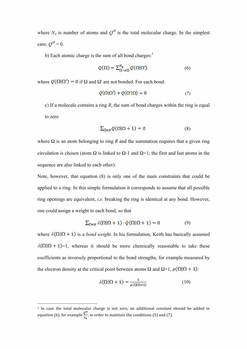
where Na is number of atoms and QM is the total molecular charge. In the simplest

case, QM = 0.

b) Each atomic charge is the sum of all bond charges:1

(6)

where if Ω and Ω' are not bonded. For each bond:

(7)

c) If a molecule contains a ring R, the sum of bond charges within the ring is equal

to zero

(8)

where Ω is an atom belonging to ring R and the summation requires that a given ring

circulation is chosen (atom Ω is linked to Ω-1 and Ω+1; the first and last atoms in the

sequence are also linked to each other).

Note, however, that equation (8) is only one of the main constraints that could be

applied to a ring. In this simple formulation it corresponds to assume that all possible

ring openings are equivalent, i.e. breaking the ring is identical at any bond. However,

one could assign a weight to each bond, so that

(9)

where is a bond weight. In his formulation, Keith has basically assumed

=1, whereas it should be more chemically reasonable to take these

coefficients as inversely proportional to the bond strengths, for example measured by

the electron density at the critical point between atoms Ω and Ω+1, :

(10)

1 In case the total molecular charge is not zero, an additional constant should be added in equation (6), for example , in order to maintain the conditions (5) and (7).

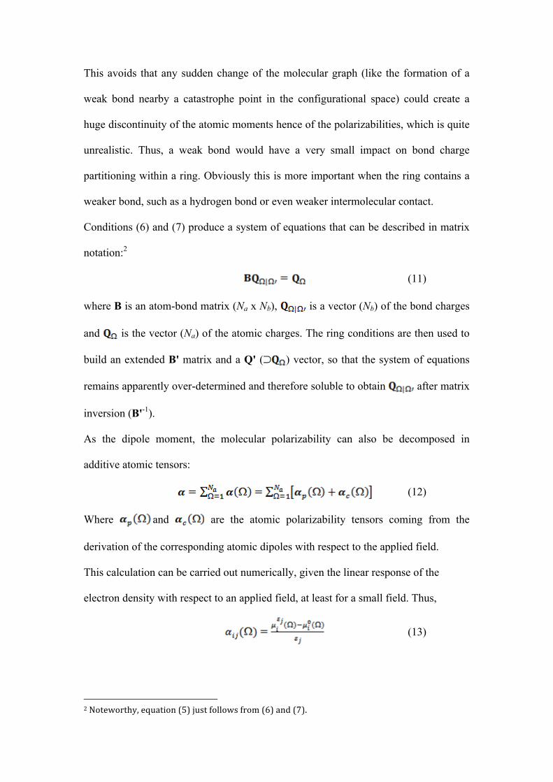
This avoids that any sudden change of the molecular graph (like the formation of a

weak bond nearby a catastrophe point in the configurational space) could create a

huge discontinuity of the atomic moments hence of the polarizabilities, which is quite

unrealistic. Thus, a weak bond would have a very small impact on bond charge

partitioning within a ring. Obviously this is more important when the ring contains a

weaker bond, such as a hydrogen bond or even weaker intermolecular contact.

Conditions (6) and (7) produce a system of equations that can be described in matrix

notation:2

(11)

where B is an atom-bond matrix (Na x Nb), is a vector (Nb) of the bond charges

and is the vector (Na) of the atomic charges. The ring conditions are then used to

build an extended B' matrix and a Q' (⊃ ) vector, so that the system of equations

remains apparently over-determined and therefore soluble to obtain after matrix

inversion (B'-1).

As the dipole moment, the molecular polarizability can also be decomposed in

additive atomic tensors:

(12)

Where and are the atomic polarizability tensors coming from the

derivation of the corresponding atomic dipoles with respect to the applied field.

This calculation can be carried out numerically, given the linear response of the

electron density with respect to an applied field, at least for a small field. Thus,

(13)

2 Noteworthy, equation (5) just follows from (6) and (7).

where is the atomic dipolar component along the i direction computed with a

given electric field (0 or ) in direction j. In general, we have used calculation at ±

and computed the derivatives by averaging the two dipole differences. Moreover, is

a sufficiently small electric field (typically 0.005 a.u.) to guarantee a better extraction

of the linear component of the electron polarization. For sake of simplicity, we do not

take into account the coupling of atomic volume and atomic charge in evaluation of

the dipole derivative. For this reason, the atomic polarizability tensors might result

slightly asymmetric (depending on the point group symmetry of the atomic basin).

This problem however, can be easily corrected through tensor symmetrization as

recommended by Nye (1985). This is obtained from decomposing of the tensor α into

symmetric (αS) and antisymmetric (αAS) terms.

(14)

(15)

As demonstrated in Table 1, this procedure reconstructs very accurately the total

molecular polarizabilities (having the molecular polarizability from analytic energy

derivatives as an exact benchmark). As a matter of facts, the antisymmetric

components are basically cancelled each other when atomic components are summed

up.

Noteworthy, all previous attempts to derive atomic polarizabilities from QTAIM

partitioning reported only diagonal components of the atomic polarization tensors.

The symmetrized atomic polarizabilities are positive tensors and can be quite easily

visualized in real space as ellipsoids, which axes have dimensions of volumes.

Moreover, they can be easily exported from atoms calculated in simple molecules to

atoms belonging to more complex systems (macromolecules or polymers, for

example). What is necessary is the definition of a proper local coordinate system that

allows exporting the atomic parameters, see for example the discussion in Domagała,

& Jelsch (2008). This is in keeping with what is generally proposed for transferable

multipolar expanded atomic electron densities, based on experimentally determined

parameters (Pichon-Pesme et al. (2004); Pichon-Pesme, Lecomte, & Lachekar (1995)

Zarychta et al. (2007)) or theoretically calculated parameters (Volkov et al. (2004),

Dittrich, B., Koritsanszky, T. & Luger, P. (2004); Dittrich et al. (2006) and Dominiak

et al. (2007)). Thus, our proposal could simply complement the known transferability

of multipolar electron density, including dipolar polarizability and it could be very

easily implemented in the existing software. However, the transferable parameters

should come from theoretical calculations.

Computational details

For a set of molecules analyzed in this paper, molecular wave functions were

calculated at B3LYP/6-311++G(2p,2d) level, using Gaussian09. For di-carboxylic

acids geometries were optimized and second derivatives of the energies were

computed in order to calculate analytically the vibrational frequencies and the

molecular polarizabilities. In case of aminoacids atomic coordinates were taken from

neutron diffraction data and kept frozen for further calculations.

The static electron density distribution was also calculated with the same method at

zero field as well as under small (0.005 a.u.) electric fields directed ( 1,0,0), (0, 1,0)

and (0,0, 1), respectively. This field was proven to be sufficiently small to obtain

good numerical derivative of the dipolar density, but for glycine, where a field of

0.001 a.u. was necessary for a precise calculation.

It is interesting that the numerical derivative we applied (through 13) is also quite a

rapid procedure to obtain molecular polarizabilities, because it requires only 7 single

point calculations under electric field and relative integration of the electron density.

The QTAIM partitioning was applied using AIMAll software. Calculation of bond

charges, atomic dipolar moments and dipolar polarizabilities was carried out with a

locally developed routine (PolaBer) that will be described in details elsewhere.

Visualization of the polarizability tensors was also carried out using a locally

developed tool, which generates a X3D file representing the data as a 3D scene. The

tensors are visualized in the same R3 space as the molecule, assuming that 1Å3 ≡ 1Å,

though normally a scaling factor is necessary to reduce the size of polarizability

ellipsoids for visualization purposes (the figures are produced with view3dscene, see

Kamburelis (2011). In all pictures, we used a scale factor of 0.4Å-2 for the atomic

polarizability tensors and 0.1Å-2 for the molecular polarizabilities.

Analysis of distributed atomic polarizabilities in test compounds

Using the theoretical background introduced above, we calculated QTAIM atomic

polarizabilities for a number of organic molecules with potential interest also in

material science, like amino acids, di-carboxylic acids etc. In fact, ammonium groups,

carboxylates, olefins, etc. are typical functionalities of organic linkers employed in

metal organic molecular materials, like for example metal organic frameworks.

Moreover, amino acids are themselves receiving increasing attention as materials, in

view of the intrinsic optical properties of their molecular crystals or co-crystals.

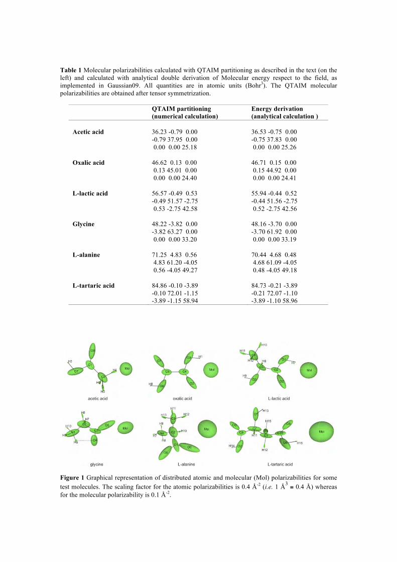
Table 1 Molecular polarizabilities calculated with QTAIM partitioning as described in the text (on the left) and calculated with analytical double derivation of Molecular energy respect to the field, as implemented in Gaussian09. All quantities are in atomic units (Bohr3). The QTAIM molecular polarizabilities are obtained after tensor symmetrization.

QTAIM partitioning (numerical calculation)

Energy derivation (analytical calculation )

Acetic acid

36.23 -0.79 0.00 -0.79 37.95 0.00 0.00 0.00 25.18

36.53 -0.75 0.00 -0.75 37.83 0.00 0.00 0.00 25.26

Oxalic acid 46.62 0.13 0.00 0.13 45.01 0.00 0.00 0.00 24.40

46.71 0.15 0.00 0.15 44.92 0.00 0.00 0.00 24.41

L-lactic acid 56.57 -0.49 0.53 -0.49 51.57 -2.75 0.53 -2.75 42.58

55.94 -0.44 0.52 -0.44 51.56 -2.75 0.52 -2.75 42.56

Glycine 48.22 -3.82 0.00 -3.82 63.27 0.00 0.00 0.00 33.20

48.16 -3.70 0.00 -3.70 61.92 0.00 0.00 0.00 33.19

L-alanine 71.25 4.83 0.56 4.83 61.20 -4.05 0.56 -4.05 49.27

70.44 4.68 0.48 4.68 61.09 -4.05 0.48 -4.05 49.18

L-tartaric acid 84.86 -0.10 -3.89 -0.10 72.01 -1.15 -3.89 -1.15 58.94

84.73 -0.21 -3.89 -0.21 72.07 -1.10 -3.89 -1.10 58.96

Figure 1 Graphical representation of distributed atomic and molecular (Mol) polarizabilities for some test molecules. The scaling factor for the atomic polarizabilities is 0.4 Å-2 (i.e. 1 Å3 ≡ 0.4 Å) whereas for the molecular polarizability is 0.1 Å-2.

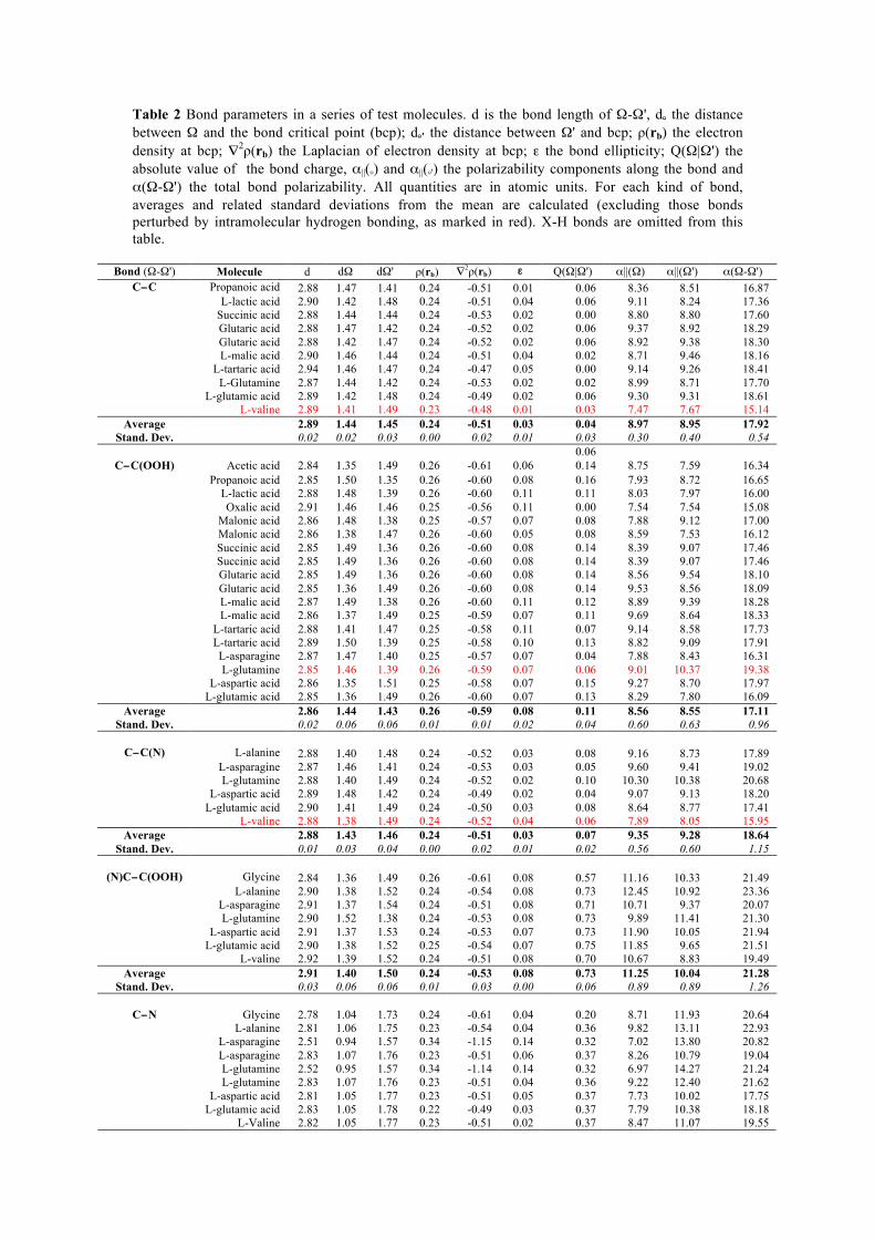
Table 2 Bond parameters in a series of test molecules. d is the bond length of Ω-Ω', dΩ the distance between Ω and the bond critical point (bcp); dΩ' the distance between Ω' and bcp; ρ(rb) the electron density at bcp; ∇2ρ(rb) the Laplacian of electron density at bcp; ε the bond ellipticity; Q(Ω|Ω') the absolute value of the bond charge, α||(Ω) and α||(Ω') the polarizability components along the bond and α(Ω-Ω') the total bond polarizability. All quantities are in atomic units. For each kind of bond, averages and related standard deviations from the mean are calculated (excluding those bonds perturbed by intramolecular hydrogen bonding, as marked in red). X-H bonds are omitted from this table.

Bond (Ω-Ω') Molecule d dΩ dΩ' ρ(rb) ∇2ρ(rb) ε Q(Ω|Ω') α||(Ω) α||(Ω') α(Ω-Ω') C−C Propanoic acid 2.88 1.47 1.41 0.24 -0.51 0.01 0.06 8.36 8.51 16.87

L-lactic acid 2.90 1.42 1.48 0.24 -0.51 0.04 0.06 9.11 8.24 17.36 Succinic acid 2.88 1.44 1.44 0.24 -0.53 0.02 0.00 8.80 8.80 17.60 Glutaric acid 2.88 1.47 1.42 0.24 -0.52 0.02 0.06 9.37 8.92 18.29 Glutaric acid 2.88 1.42 1.47 0.24 -0.52 0.02 0.06 8.92 9.38 18.30 L-malic acid 2.90 1.46 1.44 0.24 -0.51 0.04 0.02 8.71 9.46 18.16 L-tartaric acid 2.94 1.46 1.47 0.24 -0.47 0.05 0.00 9.14 9.26 18.41 L-Glutamine 2.87 1.44 1.42 0.24 -0.53 0.02 0.02 8.99 8.71 17.70 L-glutamic acid 2.89 1.42 1.48 0.24 -0.49 0.02 0.06 9.30 9.31 18.61 L-valine 2.89 1.41 1.49 0.23 -0.48 0.01 0.03 7.47 7.67 15.14

Average 2.89 1.44 1.45 0.24 -0.51 0.03 0.04 8.97 8.95 17.92 Stand. Dev. 0.02 0.02 0.03 0.00 0.02 0.01 0.03 0.30 0.40 0.54

0.06 C−C(OOH) Acetic acid 2.84 1.35 1.49 0.26 -0.61 0.06 0.14 8.75 7.59 16.34

Propanoic acid 2.85 1.50 1.35 0.26 -0.60 0.08 0.16 7.93 8.72 16.65 L-lactic acid 2.88 1.48 1.39 0.26 -0.60 0.11 0.11 8.03 7.97 16.00 Oxalic acid 2.91 1.46 1.46 0.25 -0.56 0.11 0.00 7.54 7.54 15.08 Malonic acid 2.86 1.48 1.38 0.25 -0.57 0.07 0.08 7.88 9.12 17.00 Malonic acid 2.86 1.38 1.47 0.26 -0.60 0.05 0.08 8.59 7.53 16.12 Succinic acid 2.85 1.49 1.36 0.26 -0.60 0.08 0.14 8.39 9.07 17.46 Succinic acid 2.85 1.49 1.36 0.26 -0.60 0.08 0.14 8.39 9.07 17.46 Glutaric acid 2.85 1.49 1.36 0.26 -0.60 0.08 0.14 8.56 9.54 18.10 Glutaric acid 2.85 1.36 1.49 0.26 -0.60 0.08 0.14 9.53 8.56 18.09 L-malic acid 2.87 1.49 1.38 0.26 -0.60 0.11 0.12 8.89 9.39 18.28 L-malic acid 2.86 1.37 1.49 0.25 -0.59 0.07 0.11 9.69 8.64 18.33 L-tartaric acid 2.88 1.41 1.47 0.25 -0.58 0.11 0.07 9.14 8.58 17.73 L-tartaric acid 2.89 1.50 1.39 0.25 -0.58 0.10 0.13 8.82 9.09 17.91 L-asparagine 2.87 1.47 1.40 0.25 -0.57 0.07 0.04 7.88 8.43 16.31 L-glutamine 2.85 1.46 1.39 0.26 -0.59 0.07 0.06 9.01 10.37 19.38 L-aspartic acid 2.86 1.35 1.51 0.25 -0.58 0.07 0.15 9.27 8.70 17.97 L-glutamic acid 2.85 1.36 1.49 0.26 -0.60 0.07 0.13 8.29 7.80 16.09

Average 2.86 1.44 1.43 0.26 -0.59 0.08 0.11 8.56 8.55 17.11 Stand. Dev. 0.02 0.06 0.06 0.01 0.01 0.02 0.04 0.60 0.63 0.96

C−C(N) L-alanine 2.88 1.40 1.48 0.24 -0.52 0.03 0.08 9.16 8.73 17.89

L-asparagine 2.87 1.46 1.41 0.24 -0.53 0.03 0.05 9.60 9.41 19.02 L-glutamine 2.88 1.40 1.49 0.24 -0.52 0.02 0.10 10.30 10.38 20.68 L-aspartic acid 2.89 1.48 1.42 0.24 -0.49 0.02 0.04 9.07 9.13 18.20 L-glutamic acid 2.90 1.41 1.49 0.24 -0.50 0.03 0.08 8.64 8.77 17.41 L-valine 2.88 1.38 1.49 0.24 -0.52 0.04 0.06 7.89 8.05 15.95

Average 2.88 1.43 1.46 0.24 -0.51 0.03 0.07 9.35 9.28 18.64 Stand. Dev. 0.01 0.03 0.04 0.00 0.02 0.01 0.02 0.56 0.60 1.15

(N)C−C(OOH) Glycine 2.84 1.36 1.49 0.26 -0.61 0.08 0.57 11.16 10.33 21.49

L-alanine 2.90 1.38 1.52 0.24 -0.54 0.08 0.73 12.45 10.92 23.36 L-asparagine 2.91 1.37 1.54 0.24 -0.51 0.08 0.71 10.71 9.37 20.07 L-glutamine 2.90 1.52 1.38 0.24 -0.53 0.08 0.73 9.89 11.41 21.30 L-aspartic acid 2.91 1.37 1.53 0.24 -0.53 0.07 0.73 11.90 10.05 21.94 L-glutamic acid 2.90 1.38 1.52 0.25 -0.54 0.07 0.75 11.85 9.65 21.51 L-valine 2.92 1.39 1.52 0.24 -0.51 0.08 0.70 10.67 8.83 19.49

Average 2.91 1.40 1.50 0.24 -0.53 0.08 0.73 11.25 10.04 21.28 Stand. Dev. 0.03 0.06 0.06 0.01 0.03 0.00 0.06 0.89 0.89 1.26

Glycine 2.78 1.04 1.73 0.24 -0.61 0.04 0.20 8.71 11.93 20.64

L-alanine 2.81 1.06 1.75 0.23 -0.54 0.04 0.36 9.82 13.11 22.93 L-asparagine 2.51 0.94 1.57 0.34 -1.15 0.14 0.32 7.02 13.80 20.82 L-asparagine 2.83 1.07 1.76 0.23 -0.51 0.06 0.37 8.26 10.79 19.04 L-glutamine 2.52 0.95 1.57 0.34 -1.14 0.14 0.32 6.97 14.27 21.24 L-glutamine 2.83 1.07 1.76 0.23 -0.51 0.04 0.36 9.22 12.40 21.62

L-aspartic acid 2.81 1.05 1.77 0.23 -0.51 0.05 0.37 7.73 10.02 17.75 L-glutamic acid 2.83 1.05 1.78 0.22 -0.49 0.03 0.37 7.79 10.38 18.18

C−N

L-Valine 2.82 1.05 1.77 0.23 -0.51 0.02 0.37 8.47 11.07 19.55

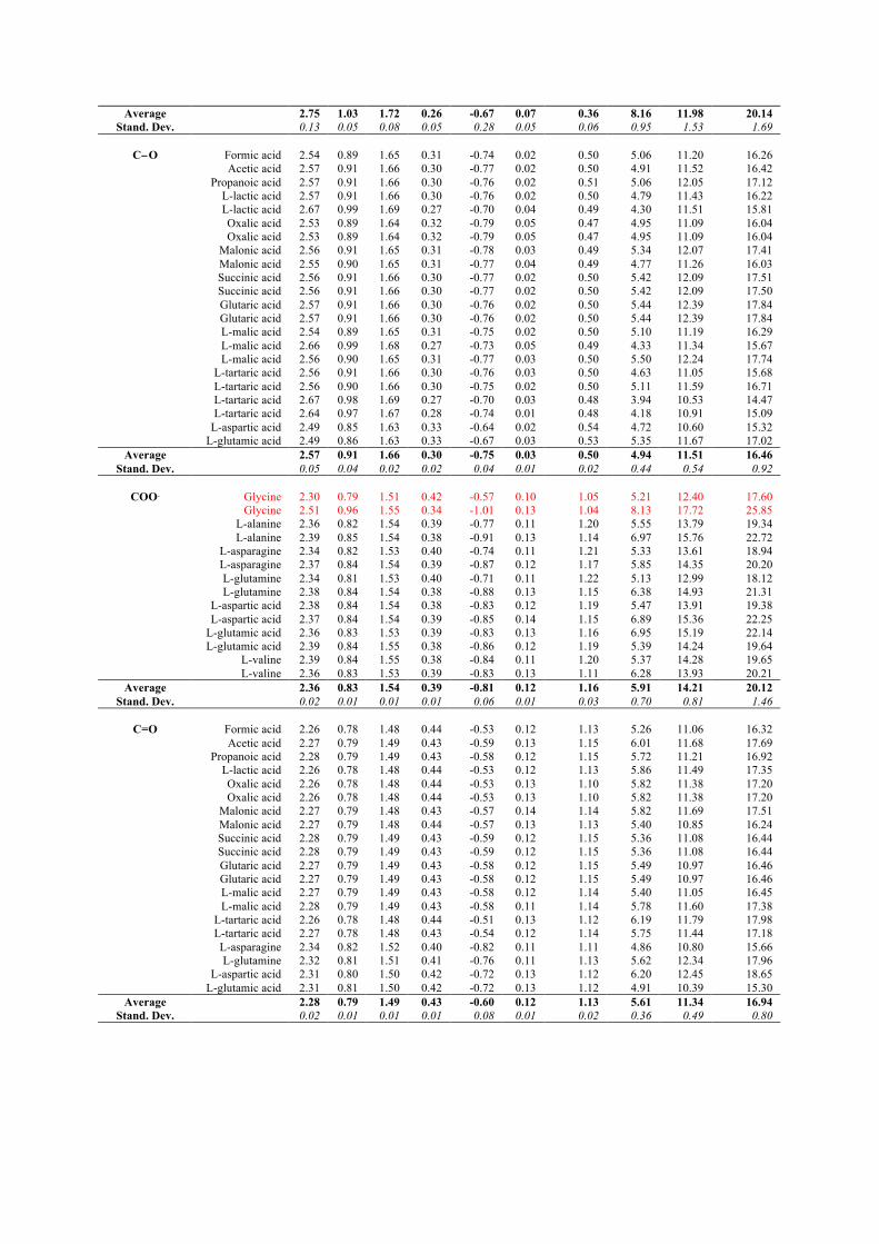
Average 2.75 1.03 1.72 0.26 -0.67 0.07 0.36 8.16 11.98 20.14 Stand. Dev. 0.13 0.05 0.08 0.05 0.28 0.05 0.06 0.95 1.53 1.69

Formic acid 2.54 0.89 1.65 0.31 -0.74 0.02 0.50 5.06 11.20 16.26 Acetic acid 2.57 0.91 1.66 0.30 -0.77 0.02 0.50 4.91 11.52 16.42

Propanoic acid 2.57 0.91 1.66 0.30 -0.76 0.02 0.51 5.06 12.05 17.12 L-lactic acid 2.57 0.91 1.66 0.30 -0.76 0.02 0.50 4.79 11.43 16.22 L-lactic acid 2.67 0.99 1.69 0.27 -0.70 0.04 0.49 4.30 11.51 15.81 Oxalic acid 2.53 0.89 1.64 0.32 -0.79 0.05 0.47 4.95 11.09 16.04 Oxalic acid 2.53 0.89 1.64 0.32 -0.79 0.05 0.47 4.95 11.09 16.04

Malonic acid 2.56 0.91 1.65 0.31 -0.78 0.03 0.49 5.34 12.07 17.41 Malonic acid 2.55 0.90 1.65 0.31 -0.77 0.04 0.49 4.77 11.26 16.03 Succinic acid 2.56 0.91 1.66 0.30 -0.77 0.02 0.50 5.42 12.09 17.51 Succinic acid 2.56 0.91 1.66 0.30 -0.77 0.02 0.50 5.42 12.09 17.50 Glutaric acid 2.57 0.91 1.66 0.30 -0.76 0.02 0.50 5.44 12.39 17.84 Glutaric acid 2.57 0.91 1.66 0.30 -0.76 0.02 0.50 5.44 12.39 17.84 L-malic acid 2.54 0.89 1.65 0.31 -0.75 0.02 0.50 5.10 11.19 16.29 L-malic acid 2.66 0.99 1.68 0.27 -0.73 0.05 0.49 4.33 11.34 15.67 L-malic acid 2.56 0.90 1.65 0.31 -0.77 0.03 0.50 5.50 12.24 17.74

L-tartaric acid 2.56 0.91 1.66 0.30 -0.76 0.03 0.50 4.63 11.05 15.68 L-tartaric acid 2.56 0.90 1.66 0.30 -0.75 0.02 0.50 5.11 11.59 16.71 L-tartaric acid 2.67 0.98 1.69 0.27 -0.70 0.03 0.48 3.94 10.53 14.47 L-tartaric acid 2.64 0.97 1.67 0.28 -0.74 0.01 0.48 4.18 10.91 15.09

L-aspartic acid 2.49 0.85 1.63 0.33 -0.64 0.02 0.54 4.72 10.60 15.32

C−O

L-glutamic acid 2.49 0.86 1.63 0.33 -0.67 0.03 0.53 5.35 11.67 17.02 Average 2.57 0.91 1.66 0.30 -0.75 0.03 0.50 4.94 11.51 16.46

Stand. Dev. 0.05 0.04 0.02 0.02 0.04 0.01 0.02 0.44 0.54 0.92

Glycine 2.30 0.79 1.51 0.42 -0.57 0.10 1.05 5.21 12.40 17.60 Glycine 2.51 0.96 1.55 0.34 -1.01 0.13 1.04 8.13 17.72 25.85

L-alanine 2.36 0.82 1.54 0.39 -0.77 0.11 1.20 5.55 13.79 19.34 L-alanine 2.39 0.85 1.54 0.38 -0.91 0.13 1.14 6.97 15.76 22.72

L-asparagine 2.34 0.82 1.53 0.40 -0.74 0.11 1.21 5.33 13.61 18.94 L-asparagine 2.37 0.84 1.54 0.39 -0.87 0.12 1.17 5.85 14.35 20.20 L-glutamine 2.34 0.81 1.53 0.40 -0.71 0.11 1.22 5.13 12.99 18.12 L-glutamine 2.38 0.84 1.54 0.38 -0.88 0.13 1.15 6.38 14.93 21.31

L-aspartic acid 2.38 0.84 1.54 0.38 -0.83 0.12 1.19 5.47 13.91 19.38 L-aspartic acid 2.37 0.84 1.54 0.39 -0.85 0.14 1.15 6.89 15.36 22.25

L-glutamic acid 2.36 0.83 1.53 0.39 -0.83 0.13 1.16 6.95 15.19 22.14 L-glutamic acid 2.39 0.84 1.55 0.38 -0.86 0.12 1.19 5.39 14.24 19.64

L-valine 2.39 0.84 1.55 0.38 -0.84 0.11 1.20 5.37 14.28 19.65

COO−

L-valine 2.36 0.83 1.53 0.39 -0.83 0.13 1.11 6.28 13.93 20.21 Average 2.36 0.83 1.54 0.39 -0.81 0.12 1.16 5.91 14.21 20.12

Stand. Dev. 0.02 0.01 0.01 0.01 0.06 0.01 0.03 0.70 0.81 1.46

Formic acid 2.26 0.78 1.48 0.44 -0.53 0.12 1.13 5.26 11.06 16.32 Acetic acid 2.27 0.79 1.49 0.43 -0.59 0.13 1.15 6.01 11.68 17.69

Propanoic acid 2.28 0.79 1.49 0.43 -0.58 0.12 1.15 5.72 11.21 16.92 L-lactic acid 2.26 0.78 1.48 0.44 -0.53 0.12 1.13 5.86 11.49 17.35 Oxalic acid 2.26 0.78 1.48 0.44 -0.53 0.13 1.10 5.82 11.38 17.20 Oxalic acid 2.26 0.78 1.48 0.44 -0.53 0.13 1.10 5.82 11.38 17.20

Malonic acid 2.27 0.79 1.48 0.43 -0.57 0.14 1.14 5.82 11.69 17.51 Malonic acid 2.27 0.79 1.48 0.44 -0.57 0.13 1.13 5.40 10.85 16.24 Succinic acid 2.28 0.79 1.49 0.43 -0.59 0.12 1.15 5.36 11.08 16.44 Succinic acid 2.28 0.79 1.49 0.43 -0.59 0.12 1.15 5.36 11.08 16.44 Glutaric acid 2.27 0.79 1.49 0.43 -0.58 0.12 1.15 5.49 10.97 16.46 Glutaric acid 2.27 0.79 1.49 0.43 -0.58 0.12 1.15 5.49 10.97 16.46 L-malic acid 2.27 0.79 1.49 0.43 -0.58 0.12 1.14 5.40 11.05 16.45 L-malic acid 2.28 0.79 1.49 0.43 -0.58 0.11 1.14 5.78 11.60 17.38

L-tartaric acid 2.26 0.78 1.48 0.44 -0.51 0.13 1.12 6.19 11.79 17.98 L-tartaric acid 2.27 0.78 1.48 0.43 -0.54 0.12 1.14 5.75 11.44 17.18 L-asparagine 2.34 0.82 1.52 0.40 -0.82 0.11 1.11 4.86 10.80 15.66 L-glutamine 2.32 0.81 1.51 0.41 -0.76 0.11 1.13 5.62 12.34 17.96

L-aspartic acid 2.31 0.80 1.50 0.42 -0.72 0.13 1.12 6.20 12.45 18.65

C=O

L-glutamic acid 2.31 0.81 1.50 0.42 -0.72 0.13 1.12 4.91 10.39 15.30 Average 2.28 0.79 1.49 0.43 -0.60 0.12 1.13 5.61 11.34 16.94

Stand. Dev. 0.02 0.01 0.01 0.01 0.08 0.01 0.02 0.36 0.49 0.80

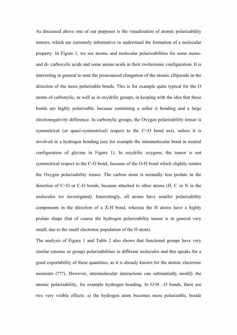
As discussed above one of our purposes is the visualization of atomic polarizability

tensors, which are extremely informative to understand the formation of a molecular

property. In Figure 1, we see atomic and molecular polarizabilities for some mono-

and di- carboxylic acids and some amino acids in their zwitterionic configuration. It is

interesting in general to note the pronounced elongation of the atomic ellipsoids in the

direction of the more polarizable bonds. This is for example quite typical for the O

atoms of carbonylic, as well as in oxydrilic groups, in keeping with the idea that these

bonds are highly polarizable, because containing a softer π bonding and a large

electronegativity difference. In carbonylic groups, the Oxygen polarizability tensor is

symmetrical (or quasi-symmetrical) respect to the C=O bond axis, unless it is

involved in a hydrogen bonding (see for example the intramolecular bond in neutral

configuration of glycine in Figure 1). In oxydrilic oxygens, the tensor is not

symmetrical respect to the C-O bond, because of the O-H bond which slightly rotates

the Oxygen polarizability tensor. The carbon atom is normally less prolate in the

direction of C=O or C-O bonds, because attached to other atoms (H, C or N in the

molecules we investigated). Interestingly, all atoms have smaller polarizability

components in the direction of a X-H bond, whereas the H atoms have a highly

prolate shape (but of course the hydrogen polarizability tensor is in general very

small, due to the small electronic population of the H atom).

The analysis of Figure 1 and Table 2 also shows that functional groups have very

similar (atomic or group) polarizabilities in different molecules and this speaks for a

good exportability of these quantities, as it is already known for the atomic electronic

moments (???). However, intermolecular interactions can substantially modify the

atomic polarizability, for example hydrogen bonding. In O-H…O bonds, there are

two very visible effects: a) the hydrogen atom becomes more polarizable, beside

normally it is more positively charged; b) the HB acceptor modifies the shape and

orientation of its polarizability tensor, which is stretched in the direction of the HB.

As we mentioned above, the presence of a ring makes the calculation of atomic

polarizabilities more arbitrary, because depending on the additional constraint

necessary for the ring. It is very interesting to compare what happens in glycine, for

both the neutral and zwitterionic configurations that we calculated. In Figure 2, we

show the distributed polarizabilites calculated using equation (8) (same scheme as

proposed by Keith), equation (9) with bond weights as defined in (10) or excluding

the hydrogen bond from the calculation. All three schemes perfectly reconstruct the

total molecular polarizability, of course, but it seems that the weighted scheme better

represents the expected continuity between a scenario with or without a weak

hydrogen bond. Noteworthy, the main changes affect the hydrogen bond acceptor

atom. The "popular" scheme (i.e. "one bond, one vote") instead drastically changes

the atomic polarizabilities, even when the hydrogen bond is very weak. For this

reason, this scheme, although equally exact, is less informative.

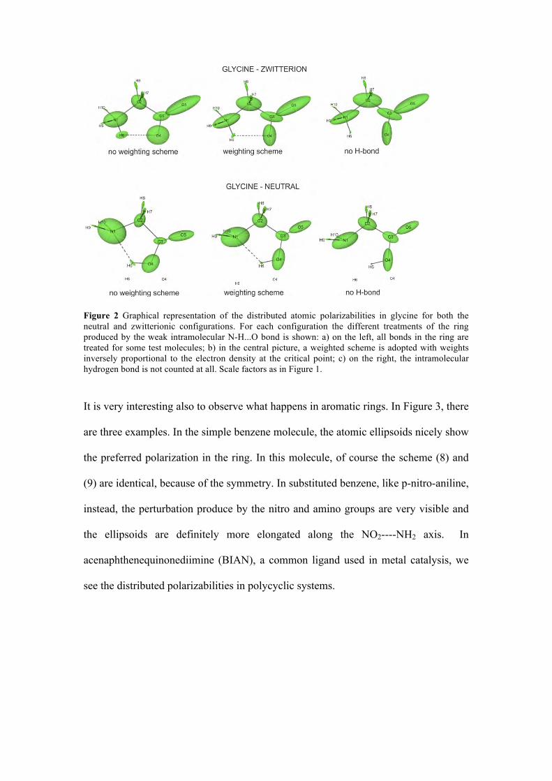
Figure 2 Graphical representation of the distributed atomic polarizabilities in glycine for both the neutral and zwitterionic configurations. For each configuration the different treatments of the ring produced by the weak intramolecular N-H...O bond is shown: a) on the left, all bonds in the ring are treated for some test molecules; b) in the central picture, a weighted scheme is adopted with weights inversely proportional to the electron density at the critical point; c) on the right, the intramolecular hydrogen bond is not counted at all. Scale factors as in Figure 1.

It is very interesting also to observe what happens in aromatic rings. In Figure 3, there

are three examples. In the simple benzene molecule, the atomic ellipsoids nicely show

the preferred polarization in the ring. In this molecule, of course the scheme (8) and

(9) are identical, because of the symmetry. In substituted benzene, like p-nitro-aniline,

instead, the perturbation produce by the nitro and amino groups are very visible and

the ellipsoids are definitely more elongated along the NO2----NH2 axis. In

acenaphthenequinonediimine (BIAN), a common ligand used in metal catalysis, we

see the distributed polarizabilities in polycyclic systems.

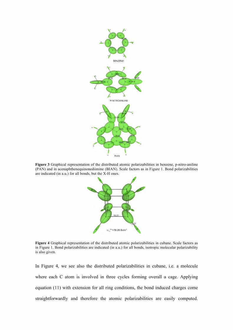
Figure 3 Graphical representation of the distributed atomic polarizabilities in benzene, p-nitro-aniline (PAN) and in acenaphthenequinonediimine (BIAN). Scale factors as in Figure 1. Bond polarizabilities are indicated (in a.u.) for all bonds, but the X-H ones.

Figure 4 Graphical representation of the distributed atomic polarizabilities in cubane. Scale factors as in Figure 1. Bond polarizabilities are indicated (in a.u.) for all bonds, isotropic molecular polarizability is also given.

In Figure 4, we see also the distributed polarizabilities in cubane, i.e. a molecule

where each C atom is involved in three cycles forming overall a cage. Applying

equation (11) with extension for all ring conditions, the bond induced charges come

straightforwardly and therefore the atomic polarizabilities are easily computed.

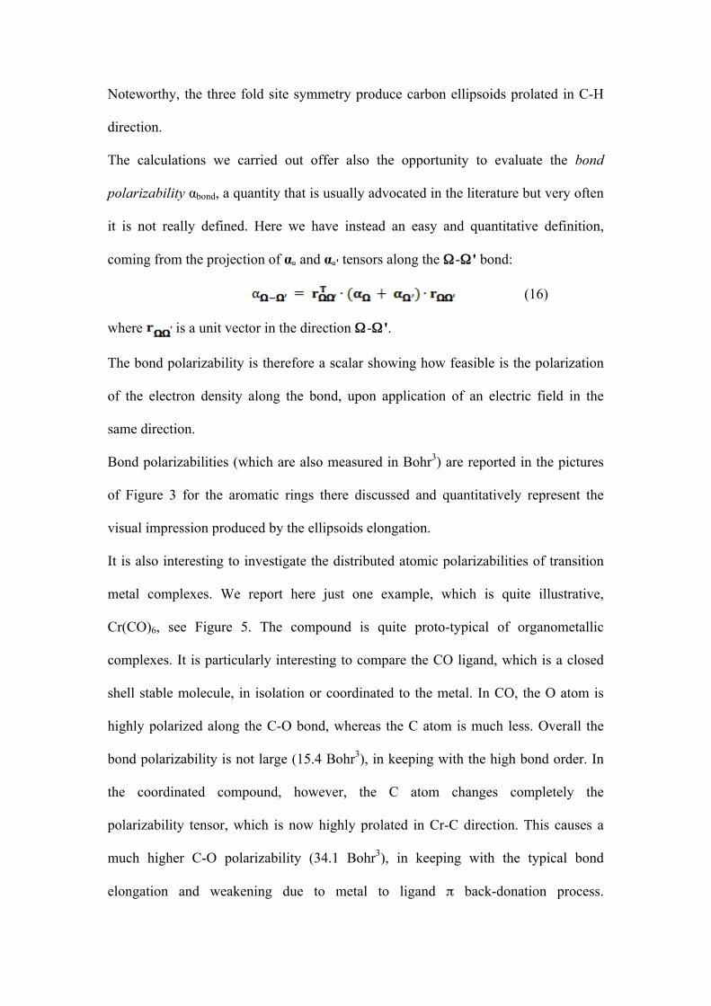
Noteworthy, the three fold site symmetry produce carbon ellipsoids prolated in C-H

direction.

The calculations we carried out offer also the opportunity to evaluate the bond

polarizability αbond, a quantity that is usually advocated in the literature but very often

it is not really defined. Here we have instead an easy and quantitative definition,

coming from the projection of αΩ and αΩ' tensors along the Ω-Ω ' bond:

(16)

where is a unit vector in the direction Ω-Ω '.

The bond polarizability is therefore a scalar showing how feasible is the polarization

of the electron density along the bond, upon application of an electric field in the

same direction.

Bond polarizabilities (which are also measured in Bohr3) are reported in the pictures

of Figure 3 for the aromatic rings there discussed and quantitatively represent the

visual impression produced by the ellipsoids elongation.

It is also interesting to investigate the distributed atomic polarizabilities of transition

metal complexes. We report here just one example, which is quite illustrative,

Cr(CO)6, see Figure 5. The compound is quite proto-typical of organometallic

complexes. It is particularly interesting to compare the CO ligand, which is a closed

shell stable molecule, in isolation or coordinated to the metal. In CO, the O atom is

highly polarized along the C-O bond, whereas the C atom is much less. Overall the

bond polarizability is not large (15.4 Bohr3), in keeping with the high bond order. In

the coordinated compound, however, the C atom changes completely the

polarizability tensor, which is now highly prolated in Cr-C direction. This causes a

much higher C-O polarizability (34.1 Bohr3), in keeping with the typical bond

elongation and weakening due to metal to ligand π back-donation process.

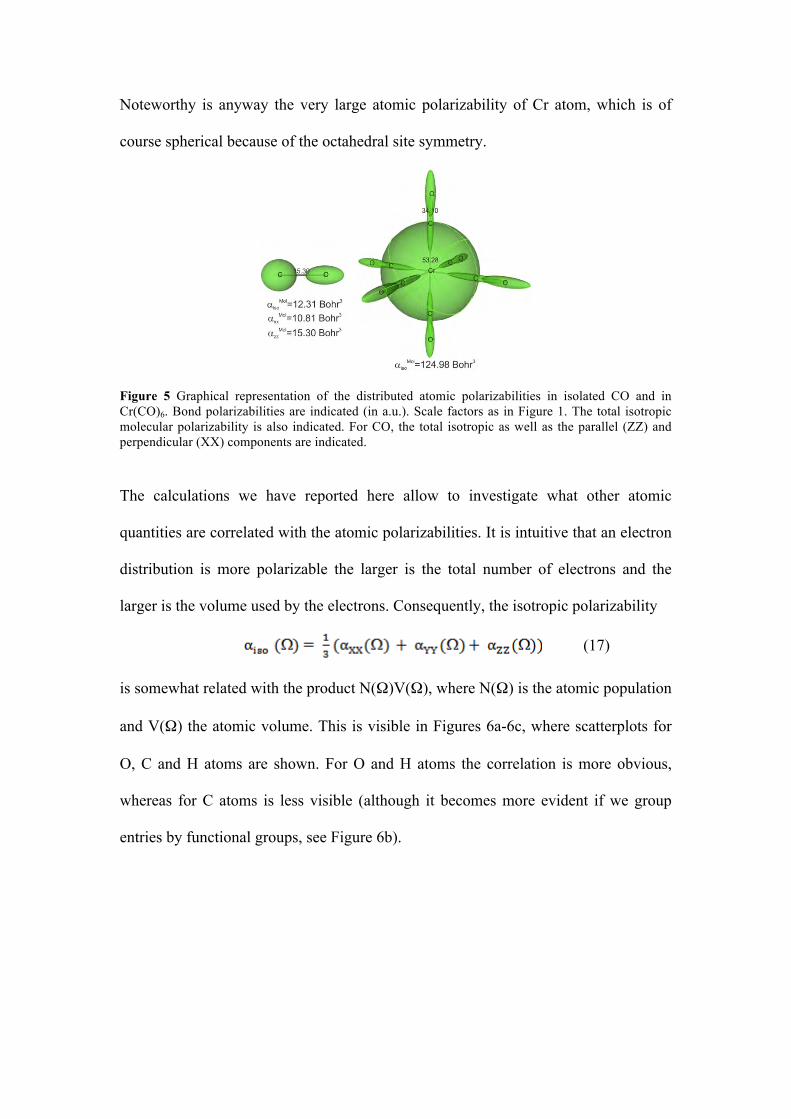
Noteworthy is anyway the very large atomic polarizability of Cr atom, which is of

course spherical because of the octahedral site symmetry.

Figure 5 Graphical representation of the distributed atomic polarizabilities in isolated CO and in Cr(CO)6. Bond polarizabilities are indicated (in a.u.). Scale factors as in Figure 1. The total isotropic molecular polarizability is also indicated. For CO, the total isotropic as well as the parallel (ZZ) and perpendicular (XX) components are indicated.

The calculations we have reported here allow to investigate what other atomic

quantities are correlated with the atomic polarizabilities. It is intuitive that an electron

distribution is more polarizable the larger is the total number of electrons and the

larger is the volume used by the electrons. Consequently, the isotropic polarizability

(17)

is somewhat related with the product N(Ω)V(Ω), where N(Ω) is the atomic population

and V(Ω) the atomic volume. This is visible in Figures 6a-6c, where scatterplots for

O, C and H atoms are shown. For O and H atoms the correlation is more obvious,

whereas for C atoms is less visible (although it becomes more evident if we group

entries by functional groups, see Figure 6b).

Figure 6 Scatterplots of isotropic atomic polarizabilities against atomic electrons x volume for Oxygen, Carbon and Hydrogen atoms calculated in the molecules reported in Table 2. The second obvious evidence is that atomic polarizability tensors are stretched in

direction of the chemical bonds, so they are directly related to the electron

polarization induced by the chemical bonding. This could be visible by comparing the

distributed atomic polarizabilities in a simple molecule, like urea, and the electron

density distribution (better emphasized by the deformation density, see Figure 7).

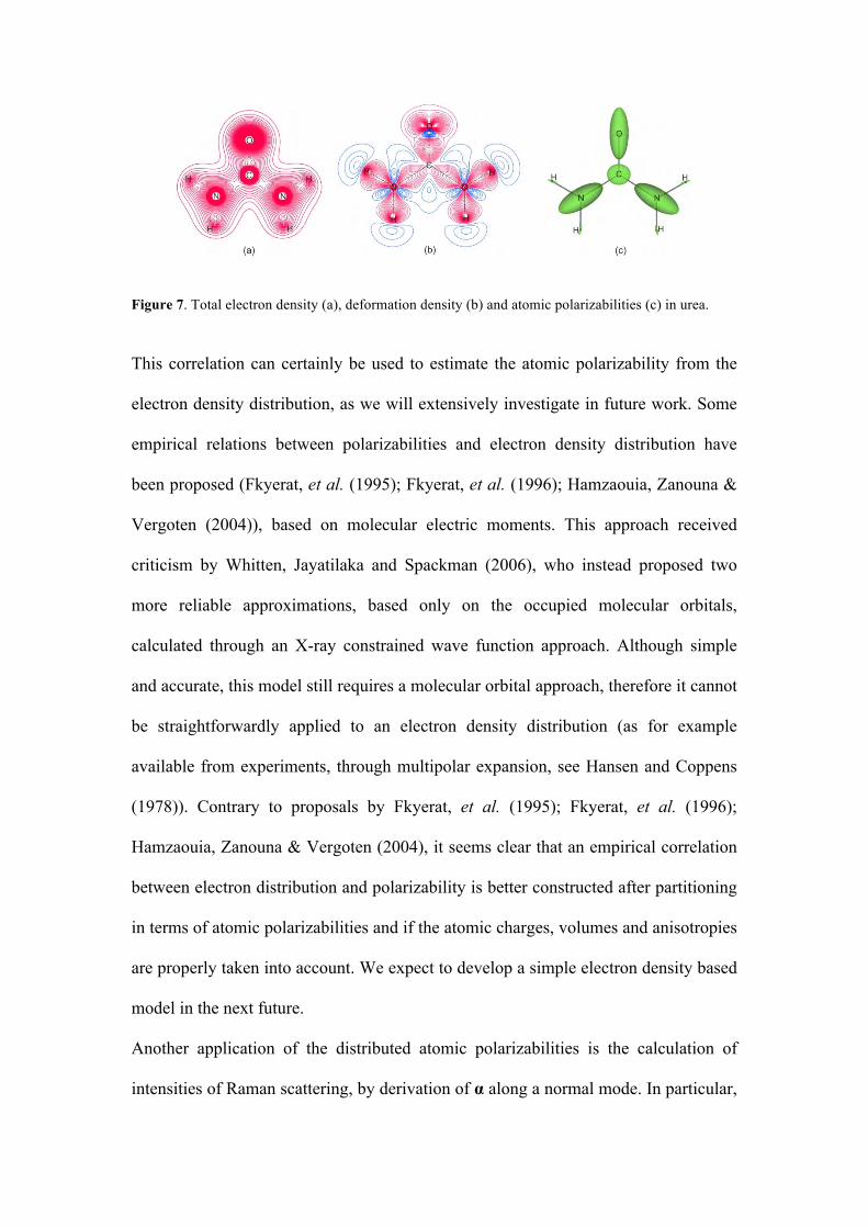
Figure 7. Total electron density (a), deformation density (b) and atomic polarizabilities (c) in urea.

This correlation can certainly be used to estimate the atomic polarizability from the

electron density distribution, as we will extensively investigate in future work. Some

empirical relations between polarizabilities and electron density distribution have

been proposed (Fkyerat, et al. (1995); Fkyerat, et al. (1996); Hamzaouia, Zanouna &

Vergoten (2004)), based on molecular electric moments. This approach received

criticism by Whitten, Jayatilaka and Spackman (2006), who instead proposed two

more reliable approximations, based only on the occupied molecular orbitals,

calculated through an X-ray constrained wave function approach. Although simple

and accurate, this model still requires a molecular orbital approach, therefore it cannot

be straightforwardly applied to an electron density distribution (as for example

available from experiments, through multipolar expansion, see Hansen and Coppens

(1978)). Contrary to proposals by Fkyerat, et al. (1995); Fkyerat, et al. (1996);

Hamzaouia, Zanouna & Vergoten (2004), it seems clear that an empirical correlation

between electron distribution and polarizability is better constructed after partitioning

in terms of atomic polarizabilities and if the atomic charges, volumes and anisotropies

are properly taken into account. We expect to develop a simple electron density based

model in the next future.

Another application of the distributed atomic polarizabilities is the calculation of

intensities of Raman scattering, by derivation of α along a normal mode. In particular,

if the mode coincide with a given bond, then it is easy to numerically differentiate the

bond polarizability αA-B (to give α'||) and therefore compute the Raman intensities and

the atomic contributions to that. For example, in CO there is only one mode (bond

stretching). The bond polarizability derivative (α'|| = 9.3 Bohr2) is directly

proportional to the Raman intensity, but C and O have different contribution to (3.2

and 6.1 Bohr2, respectively), that could be used to analyze the individual atomic

contribution to a given Raman intensity. Noteworthy, also the polarizability change

perpendicular to the bond is relevant, and can be of course calculated (α'⊥ = 1.06

Bohr2; α'⊥(C) = 0.31 Bohr2; α'⊥(O) = 0.75 Bohr2), again confirming that O has the

larger contribution.

Conclusions

In this paper, we have investigated QTAIM distributed atomic polarizabilities with

the intent to extract more chemical information from a quantity that can be calculated

with precision at quantum chemical level, but that is normally not analysed in details.

In particular, we have proposed a different and more reliable way to partition the

polarizability in case of "loops" in the molecular graph. We have also proposed a way

to visualize the atomic polarizabilities, which is extremely informative to show which

factors mostly affect these quantities. Moreover, we have introduced an indicator for

the bond polarizability, obtained as the sum of projected atomic polarizability over a

bond.

The applications of this approach are enormous and we summarize here the plan for

the near future.

Larger molecules, organometallic polymers and crystals. It appears from this study

that distributed atomic polarizabilities are quite transferable, when functional groups

are properly defined. This allows calculating semi-empirical molecular polarizabilities

for larger molecules at low costs. Corrections due to intermolecular bonding can be

easily incorporated. This could be particularly for the calculation of crystal optic

properties, like for example refractive indexes, using atomic polarizabilities for each

functional group of the molecular species.

Modelling from experimental electron density. The tight relationship between atomic

polarizabilities and atomic electron density can be further exploited trying to improve

the current empirical models that tentatively reconstruct a molecular polarizability

from multipolar expanded electron density distributions. This could facilitate the

estimation of the polarizability tensors directly from experiment.

Intermolecular energies. A better quality distributed atomic polarizabilities could be

useful for the evaluation of induction energies (interaction between external electric

field and molecular polarizability) and dispersion energies (mutual interaction

between polarizabilities) in simulations of macromolecules as well as crystal packed

species.

Hyper-polarizabilities. An extension of the current approach could provide the

distributed atomic hyper-polarizabilities, based on double (or higher) derivatives of

the dipolar density of eq. (4) with respect to the field. This would open access to

evaluation of non linear optic properties in crystal, as well.

Acknowledgements

We thank Swiss CRUS for financial support (sciex NMS boursary 10.083). Prof. D.

Jayatilaka is thanked for several useful discussions and comments.

References

Bader, R.F.W. (1989) J. Chem. Phys. 91, 6989-7001.

Bader, R.F.W. (1990) Atoms in Molecules: A Quantum Theory, Oxford University

Press, Oxford, UK, 1990.

Bader, R.F.W., Keith, T.A., Gough, K.M. & Laidig K.E. Mol. Phys. (1992) 75, 1167-

1189.

Bader, R.F.W., Larouche, A., Gatti, C., Carroll, M.T., MacDougall, P.J. & Wiberg,

K.B. (1987) J.Chem.Phys. 87, 1142-1152.

Dittrich, B., Koritsanszky, T. & Luger, P. (2004) Angew. Chem. Int. Ed. Engl. 43,

2718–2721.

Dittrich, B., Hübschle, C.B., Luger, P. & Spackman, M.A. (2006) Acta Cryst. D 62,

1325–1335.

Domagała, S. & Jelsch, C. (2008) J. Appl. Cryst. 41, 1140–1149.

Dominiak, P.M., Volkov, A., Li, X., Messerschmidt, M. & Coppens, P. (2007) J.

Chem. Theory Comput. 3, 232-247.

Fkyerat, A., Guelzim, A., Baert, F., Paulus, W., Heger, G., Zyss, J. & Périgaud, A.

(1995) Acta Cryst., B51, 197-209.

Fkyerat, A., Guelzim, A., Baert, F., Zyss, J. & Périgaud, A. (1996) Phys. Rev. B, 53,

16236-16246.

Hamzaoui, F., Zanoun, A. & Vergoten, G. (2004) Journal of Molecular Structure

697, 17–22.

Hansen, N. K. & Coppens P. (1978) Acta Cryst, A34, 909-921

Kamburelis, M. (2011) view3dscene(version 3.10.1), http://castle-

engine.sourceforge.net.

Keith, T.A. (2007) Atomic Response Properties in The Quantum Theory of Atoms in

Molecules: From Solid State to DNA and Drug Design Matta C.F., Boyd R.J., Eds.,

Wiley-VCH, Weinheim, 2007.

Keith, T.A. (2011) AIMAll, Version 11.10.16, aim.tkgristmill.com.

Nye, J.F (1985) Physical Properties of Crystals: Their Representation by Tensors and

Matrices, Oxford University Press.

Laidig K.E. & Bader. R.F.W. (1990) J. Chem. Phys. 93, 7213-7224.

Le Sueur, C.R. & Stone, A.J. (1993) Molecular Physics, 78, 1267-1291.

Pichon-Pesme, V., Jelsch, C., Guillot, B. & Lecomte, C. (2004) Acta Cryst. A 60,

204-208.

Pichon-Pesme, V., Lecomte, C. & Lachekar, H. (1995) J. Phys. Chem., 99, 6242–

6250.

Stone, A. J. (1985) Molecular Physics, 56, 1065-1082.

Volkov, A., Li, X., Koritsanszky, T. & Coppens, P. (2004) J. Phys. Chem. A 108,

4283-4300.

Whitten, A.E., Jayatilaka, D. & Spackman, M.A. (2006) J. Chem. Phys., 125, 174505-

174515.

Zarychta, B., Pichon-Pesme, V., Guillot, B., Lecomte C. & Jelsch C. (2007) Acta

Cryst. A63, 108-125.

CHARACTERIZATION OF WEAK INTRA- AND INTERMOLECULAR INTERACTIONS USING EXPERIMENTAL CHARGE DENSITY DISTRIBUTIONS

Edwin D. Stevens and MaRyca Watts Department of Chemistry, University of New Orleans, New Orleans, LA 70148, USA

ABSTRACT It is now possible to obtain the electronic structures of crystalline solids using high-

resolution x-ray diffraction measurements on an almost routine basis. In many cases, remarkable agreement has been obtained between experimental measurements on molecular solids and charge densities calculated with large basis set ab initio or density functional theoretical methods. Topological analysis of both experimental and theoretical charge density distributions using the Atoms in Molecules (AIM) theory is now common, and provides further insight into features of the charge distribution associated with inter-atomic interactions.

In recent studies, we have obtained experimental charge density distributions of several molecular solids, including the disaccharides α,α-trehalose and methyl-β-cellobioside, the natural product gossypol, and several small organic molecules which show topological evidence of a variety of weak interactions. In addition to conventional hydrogen bonds, bond paths and bond critical points corresponding to C-H … O hydrogen bonds are frequently observed. Other observed interactions are perhaps better characterized as van der Waals contacts. Theoretical density functional calculations of molecular clusters confirm the interactions observed in the experimental charge distributions, but in some cases show additional interactions which are presumably too weak to be observed experimentally.

Also of interest is the experimental charge distribution in molecules where the electronic structure and molecular geometry are influenced by the anomeric and/or the exo-anomeric effect. Examination of bond distances and the electron density at the bond critical points in bonds subject of the anomeric effect in sucrose, trehalose, and methyl-cellobioside yield differences which are generally consistent with the electronic model in which lone pair donation to a sigma antibonding orbital is responsible for the anomeric effect.

Since the experimental results on the disaccharides α,α-trehalose and methyl-β-cellobioside and the natural product gossypol have either been published, or will shortly be published elsewhere, this contribution will focus in detail on the experimental electron density distributions of maleic anhydride and maleic acid. Both molecules are small enough to allow future accurate theoretical calculations of the electron distribution in the crystalline environment for comparison with the experimental results.

INTRODUCTION The use of accurate, high-resolution x-ray diffraction intensity measurements to obtain the electron density distributions of solids is well established [1,2]. In most cases, experimental studies have focused on the major features of the electronic structure, the deformation of the atomic density as a result of ionic or covalent bond formation. Changes in the charge density associated with hydrogen bonding, one of the strongest intermolecular interactions, have also received considerable attention. With continued improvements in accuracy of experimental techniques, as well as improved methods for the refinement an analysis of experimental results, evidence in the electron density distribution for weaker interactions, both within and between molecules, has become apparent. Foremost among these weaker interactions are C-H … O hydrogen bonds, for which extensive structural evidence exists [3]. Interpretation of features of the electron density distribution has been assisted by a synergistic interaction between experimental results and theoretical calculations. The incorporation of density functional corrections into ab initio theoretical programs has made the calculation of high quality theoretical densities of isolated molecules possible, even for non-specialists [4]. In addition, the effects of the crystal environment can be included using calculations with periodic boundary conditions, calculations using nearest-neighbor fragments, or clusters coupled to environments treated at the semi-empirical level. Another significant development has been the use of topological analysis, specifically Bader’s Quantum Theory of Atoms in Molecules (AIM), for the analysis of both experimental and theoretical electron density distributions [5]. A common analysis method allows a more direct comparison of experimental and experimental densities in terms of a modest number of critical points which are characteristic of a particular distribution. Included in this study are some recent experimental results obtained in our laboratories which have focused on weak intra- and intermolecular interactions. Similar interactions have been observed by other investigators in a wide variety of experimental and theoretical studies. DENSITY REFINEMENT AND ANALYSIS Given an accurate set of experimental x-ray structure factors, Fh, the three-dimensional electron density distribution in a crystal, ρ(r), can be calculated using a Fourier series summation, ρ(r) = Σh Fh e2πih.r . However, the density calculated in this manner will suffer from a number of limitations. Since only a finite number of unique observations are possible, the density will contain series termination errors. Also, since there are experimental errors associated with the x-ray intensity measurements, the density distribution will include experimental noise (which increases as the number of observations is increased). Finally, the density will correspond to an average over the atomic displacements due to the modes of thermal motion at the temperature of the data collection. To avoid these problems, the electron density distribution is typically obtained by a multipole least-squares refinement of the x-ray data in which parameters describing the

distortions of the electron density from that of a collection of neutral, spherical atoms are included as refinable variables. The atomic density model, as incorporated in the Hansen-Coppens formalism [6] is given by the expression ρatom(r) = ρcore(r) + Pvalence ρvalence(κ r) + Σl,m Pl,m Rl(κ′r) Yl,m(θ,φ), where ρcore(r) is the density of the core electrons, ρvalence(r) is the spherical density of the valence electrons, and Rl(r) and Yl,m(θ,φ) are radial and spherical harmonic angular functions describing the distortions of the density from that of a spherical atom. Values of the parameters Pvalence, Pl,m, and the expansion/contraction parameters κ and κ′ are obtained by the weighted least-squares refinement using the XD2006 computer program [7]. One measure of the success of the multipole refinement is a plot of the residual density, obtained by a Fourier series summation of the difference between the experimental structure factors and the structure factors calculated from the multipole model. If the multipole model is adequate, the residual density should contain only random features resulting from errors in the experimental data. After refinement of the multipole model, the molecular density can be plotted directly, avoiding series termination errors and noise due to random errors in the x-ray measurements. In addition, if the model for thermal motion is adequate, then the multipole model density calculated without the atomic thermal probability distributions is an estimate of the static molecular electron density. The resulting static multipole model density is given by ∆ρ(r) = ρmultipole model - ρspherical atoms. Features of the deformation density thus always compare the observed density to a reference density, which is the density calculated for a collection of neutral, non-interacting spherical atomic densities. One advantage of AIM topological analysis is the use of the total electron density, and thus the absence of the need for a reference density. Topological properties of the experimental electron density distribution of interest in the study of weak intermolecular interactions include the locations of bond critical points (BCPs), the total electron density, ρ(rb), and Laplacian of the density, ∇2ρ(rb), at the BCPs, and the atomic volume and charge integrated over the atomic basins. In most cases, estimated standard deviations in the properties are available and are calculated based on the uncertainties of the multipole population parameters obtained by least-squares refinement of the X-ray data. The topological properties at the bond critical points can be used to estimate the interaction energies associated with weak intra- and intermolecular interactions. Abramov [8] has proposed density functionals for the local kinetic energy, the local potential energy and from them the binding energy of a hydrogen bond or other closed shell interaction. The local kinetic energy is given by G(rb) = (3/10)(3π2)3/2[ρ(rb)]5/3 + (1/6) ∇2ρ(rb), the local potential energy by V(rb) = (1/4) ∇2ρ(rb) – 2 G(rb), and the binding energy by EHB = - ½ V(rb). Also, since the topological properties of the electron density in non-covalent interactions are found to depend exponentially on the d(H … A) donor-acceptor distance, it is not surprising that the energy calculated from the topological properties would also show an exponential dependence on the

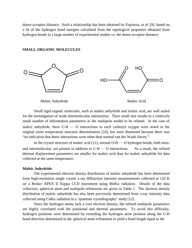
donor-acceptor distance. Such a relationship has been obtained by Espinosa, et al. [9], based on a fit of the hydrogen bond energies calculated from the topological properties obtained from hydrogen bonds in a large number of experimental studies vs. the donor-acceptor distance. SMALL ORGANIC MOLECULES

Maleic Anhydride Maleic Acid Small rigid organic molecules, such as maleic anhydride and maleic acid, are well suited for the investigation of weak intermolecular interactions. Their small size results in a relatively small number of deformation parameters in the multipole model to be refined. In the case of maleic anhydride, three C-H … O interactions to each carbonyl oxygen were noted in the original room temperature structure determination [10], but were dismissed because there was “no indication that these interactions were other than normal van der Waals forces.” In the crystal structure of maleic acid [11], normal O-H … O hydrogen bonds, both intra- and intermolecular, are present in addition to C-H … O interactions. As a result, the refined thermal displacement parameters are smaller for maleic acid than for maleic anhydride for data collected at the same temperature. Maleic Anhydride The experimental electron density distribution of maleic anhydride has been determined from high-resolution single crystal x-ray diffraction intensity measurements collected at 120 K on a Bruker APEX II Kappa CCD instrument using MoKα radiation. Details of the data collection, spherical atom and multipole refinement are given in Table 1. The electron density distribution of maleic anhydride has also been previously determined from x-ray intensity data collected using CuKα radiation in a ‘quantum crystallography’ study [12]. Since the hydrogen atoms lack a core electron density, the refined multipole parameters are highly correlated with the positional and thermal parameters. To avoid this difficulty, hydrogen positions were determined by extending the hydrogen atom position along the C-H bond direction determined in the spherical atom refinement to yield a bond length equal to the

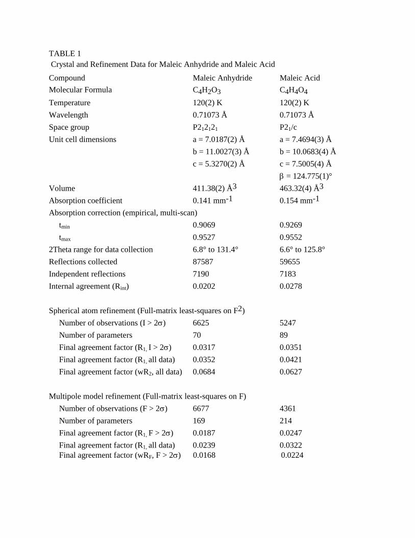
TABLE 1 Crystal and Refinement Data for Maleic Anhydride and Maleic Acid

Compound Maleic Anhydride Maleic Acid Molecular Formula C4H2O3 C4H4O4 Temperature 120(2) K 120(2) K Wavelength 0.71073 Å 0.71073 Å

Space group P212121 P21/c Unit cell dimensions a = 7.0187(2) Å a = 7.4694(3) Å b = 11.0027(3) Å b = 10.0683(4) Å c = 5.3270(2) Å c = 7.5005(4) Å β = 124.775(1)° Volume 411.38(2) Å3 463.32(4) Å3

Absorption coefficient 0.141 mm-1 0.154 mm-1 Absorption correction (empirical, multi-scan) tmin 0.9069 0.9269 tmax 0.9527 0.9552 2Theta range for data collection 6.8° to 131.4° 6.6° to 125.8° Reflections collected 87587 59655 Independent reflections 7190 7183 Internal agreement (Rint) 0.0202 0.0278 Spherical atom refinement (Full-matrix least-squares on F2) Number of observations (I > 2σ) 6625 5247 Number of parameters 70 89 Final agreement factor (R1, I > 2σ) 0.0317 0.0351 Final agreement factor (R1, all data) 0.0352 0.0421 Final agreement factor (wR2, all data) 0.0684 0.0627 Multipole model refinement (Full-matrix least-squares on F) Number of observations (F > 2σ) 6677 4361 Number of parameters 169 214 Final agreement factor (R1, F > 2σ) 0.0187 0.0247 Final agreement factor (R1, all data) 0.0239 0.0322 Final agreement factor (wRF, F > 2σ) 0.0168 0.0224

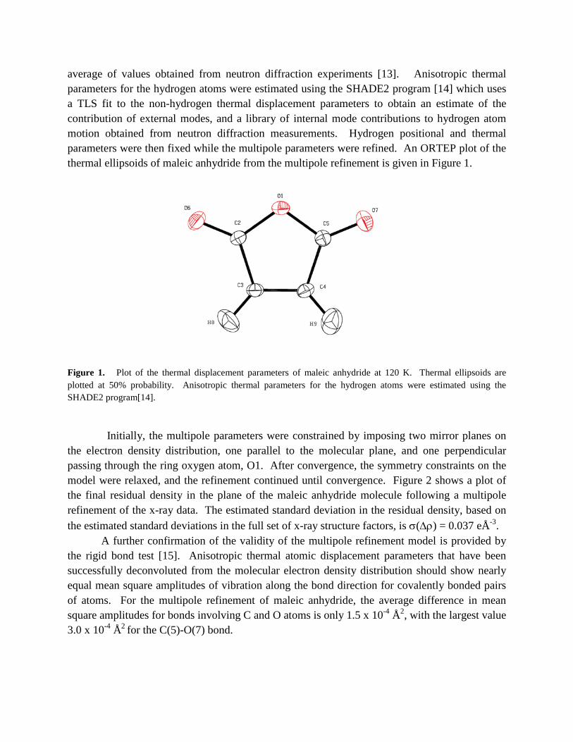
average of values obtained from neutron diffraction experiments [13]. Anisotropic thermal parameters for the hydrogen atoms were estimated using the SHADE2 program [14] which uses a TLS fit to the non-hydrogen thermal displacement parameters to obtain an estimate of the contribution of external modes, and a library of internal mode contributions to hydrogen atom motion obtained from neutron diffraction measurements. Hydrogen positional and thermal parameters were then fixed while the multipole parameters were refined. An ORTEP plot of the thermal ellipsoids of maleic anhydride from the multipole refinement is given in Figure 1.

Figure 1. Plot of the thermal displacement parameters of maleic anhydride at 120 K. Thermal ellipsoids are plotted at 50% probability. Anisotropic thermal parameters for the hydrogen atoms were estimated using the SHADE2 program[14].

Initially, the multipole parameters were constrained by imposing two mirror planes on the electron density distribution, one parallel to the molecular plane, and one perpendicular passing through the ring oxygen atom, O1. After convergence, the symmetry constraints on the model were relaxed, and the refinement continued until convergence. Figure 2 shows a plot of the final residual density in the plane of the maleic anhydride molecule following a multipole refinement of the x-ray data. The estimated standard deviation in the residual density, based on the estimated standard deviations in the full set of x-ray structure factors, is σ(∆ρ) = 0.037 eÅ-3.

A further confirmation of the validity of the multipole refinement model is provided by the rigid bond test [15]. Anisotropic thermal atomic displacement parameters that have been successfully deconvoluted from the molecular electron density distribution should show nearly equal mean square amplitudes of vibration along the bond direction for covalently bonded pairs of atoms. For the multipole refinement of maleic anhydride, the average difference in mean square amplitudes for bonds involving C and O atoms is only 1.5 x 10-4 Å2, with the largest value 3.0 x 10-4 Å2 for the C(5)-O(7) bond.

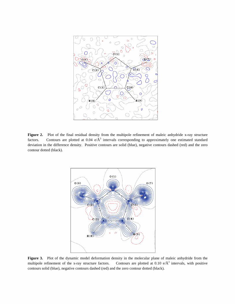
Figure 2. Plot of the final residual density from the multipole refinement of maleic anhydride x-ray structure factors. Contours are plotted at 0.04 e/Å3 intervals corresponding to approximately one estimated standard deviation in the difference density. Positive contours are solid (blue), negative contours dashed (red) and the zero contour dotted (black).

Figure 3. Plot of the dynamic model deformation density in the molecular plane of maleic anhydride from the multipole refinement of the x-ray structure factors. Contours are plotted at 0.10 e/Å3 intervals, with positive contours solid (blue), negative contours dashed (red) and the zero contour dotted (black).

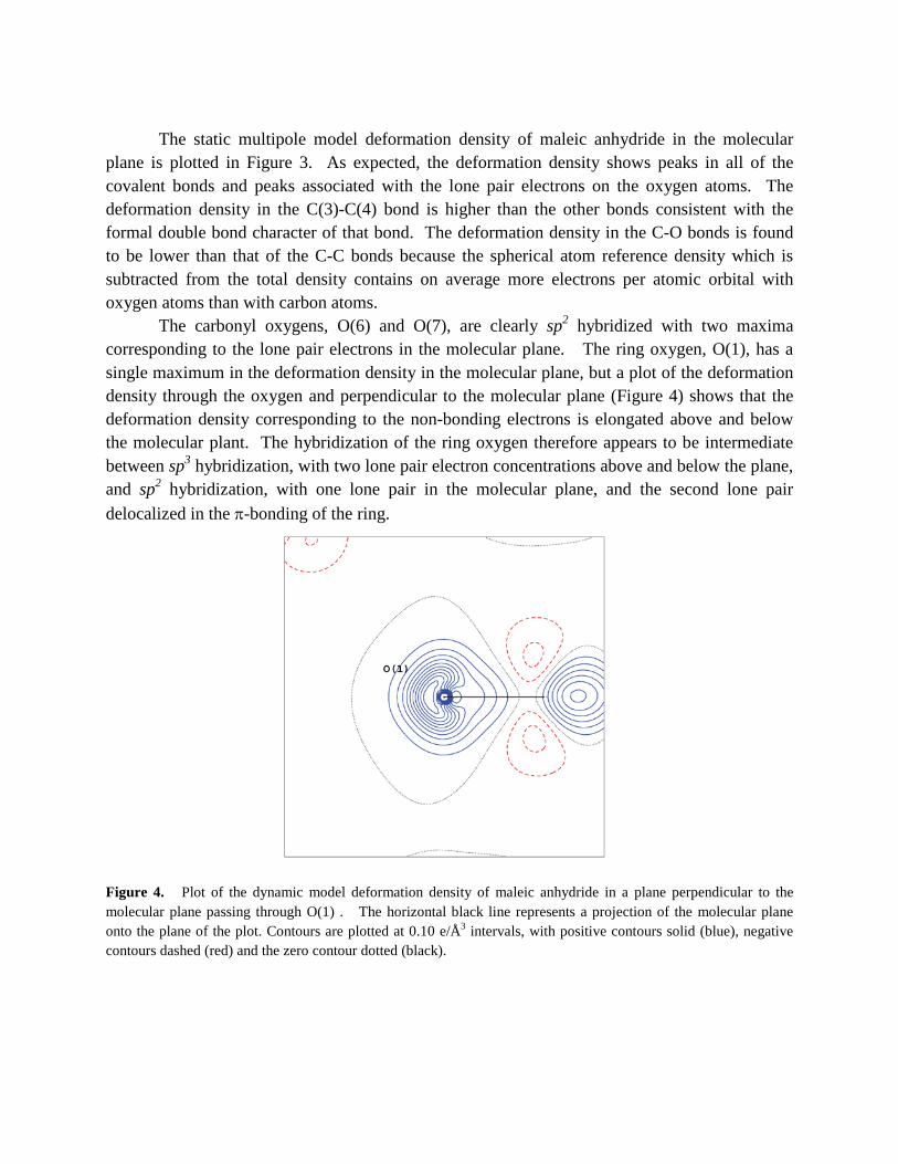
The static multipole model deformation density of maleic anhydride in the molecular

plane is plotted in Figure 3. As expected, the deformation density shows peaks in all of the covalent bonds and peaks associated with the lone pair electrons on the oxygen atoms. The deformation density in the C(3)-C(4) bond is higher than the other bonds consistent with the formal double bond character of that bond. The deformation density in the C-O bonds is found to be lower than that of the C-C bonds because the spherical atom reference density which is subtracted from the total density contains on average more electrons per atomic orbital with oxygen atoms than with carbon atoms.

The carbonyl oxygens, O(6) and O(7), are clearly sp2 hybridized with two maxima corresponding to the lone pair electrons in the molecular plane. The ring oxygen, O(1), has a single maximum in the deformation density in the molecular plane, but a plot of the deformation density through the oxygen and perpendicular to the molecular plane (Figure 4) shows that the deformation density corresponding to the non-bonding electrons is elongated above and below the molecular plant. The hybridization of the ring oxygen therefore appears to be intermediate between sp3 hybridization, with two lone pair electron concentrations above and below the plane, and sp2 hybridization, with one lone pair in the molecular plane, and the second lone pair delocalized in the π-bonding of the ring.

Figure 4. Plot of the dynamic model deformation density of maleic anhydride in a plane perpendicular to the molecular plane passing through O(1) . The horizontal black line represents a projection of the molecular plane onto the plane of the plot. Contours are plotted at 0.10 e/Å3 intervals, with positive contours solid (blue), negative contours dashed (red) and the zero contour dotted (black).

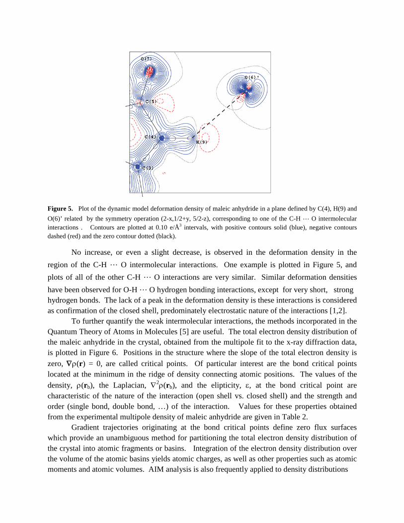
Figure 5. Plot of the dynamic model deformation density of maleic anhydride in a plane defined by C(4), H(9) and O(6)’ related by the symmetry operation (2-x,1/2+y, 5/2-z), corresponding to one of the C-H … O intermolecular interactions . Contours are plotted at 0.10 e/Å3 intervals, with positive contours solid (blue), negative contours dashed (red) and the zero contour dotted (black).

No increase, or even a slight decrease, is observed in the deformation density in the region of the C-H … O intermolecular interactions. One example is plotted in Figure 5, and plots of all of the other C-H … O interactions are very similar. Similar deformation densities have been observed for O-H … O hydrogen bonding interactions, except for very short, strong hydrogen bonds. The lack of a peak in the deformation density is these interactions is considered as confirmation of the closed shell, predominately electrostatic nature of the interactions [1,2]. To further quantify the weak intermolecular interactions, the methods incorporated in the Quantum Theory of Atoms in Molecules [5] are useful. The total electron density distribution of the maleic anhydride in the crystal, obtained from the multipole fit to the x-ray diffraction data, is plotted in Figure 6. Positions in the structure where the slope of the total electron density is zero, ∇ρ(r) = 0, are called critical points. Of particular interest are the bond critical points located at the minimum in the ridge of density connecting atomic positions. The values of the density, ρ(rb), the Laplacian, ∇2ρ(rb), and the elipticity, ε, at the bond critical point are characteristic of the nature of the interaction (open shell vs. closed shell) and the strength and order (single bond, double bond, …) of the interaction. Values for these properties obtained from the experimental multipole density of maleic anhydride are given in Table 2. Gradient trajectories originating at the bond critical points define zero flux surfaces which provide an unambiguous method for partitioning the total electron density distribution of the crystal into atomic fragments or basins. Integration of the electron density distribution over the volume of the atomic basins yields atomic charges, as well as other properties such as atomic moments and atomic volumes. AIM analysis is also frequently applied to density distributions

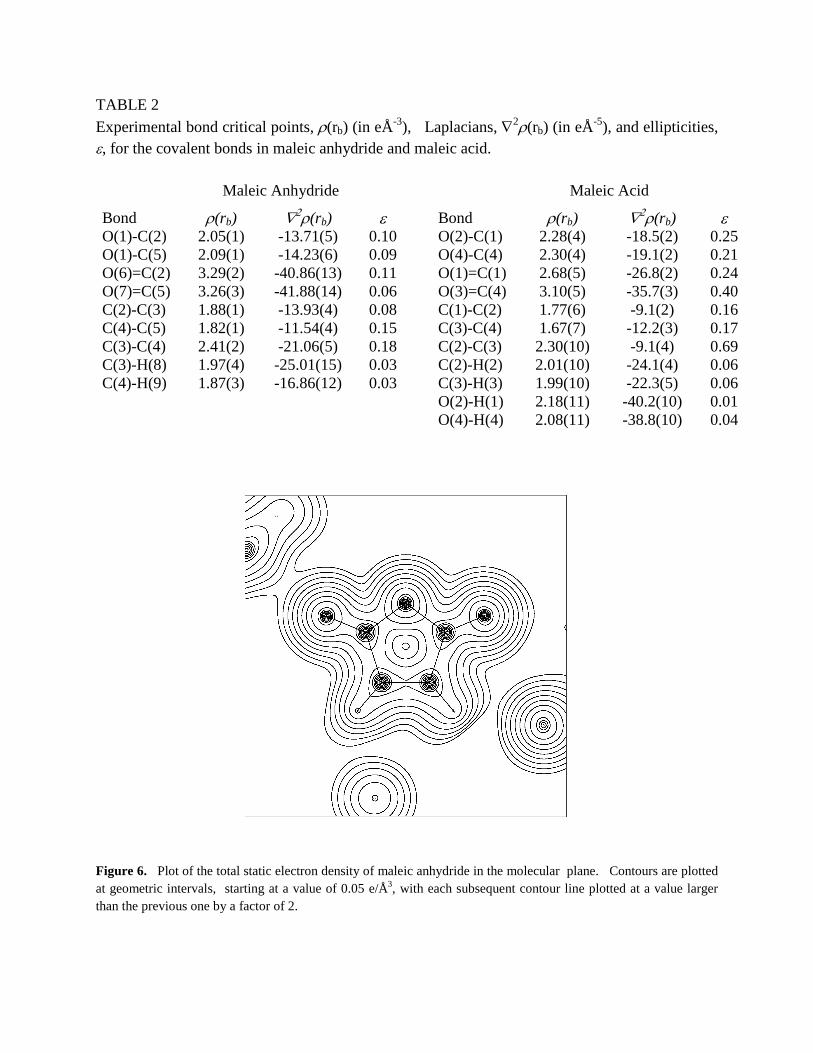
TABLE 2 Experimental bond critical points, ρ(rb) (in eÅ-3), Laplacians, ∇2ρ(rb) (in eÅ-5), and ellipticities, ε, for the covalent bonds in maleic anhydride and maleic acid.

Maleic Anhydride

Maleic Acid

Bond ρ(rb) ∇2ρ(rb) ε

Bond ρ(rb) ∇2ρ(rb) ε O(1)-C(2) 2.05(1) -13.71(5) 0.10

O(2)-C(1) 2.28(4) -18.5(2) 0.25

O(1)-C(5) 2.09(1) -14.23(6) 0.09

O(4)-C(4) 2.30(4) -19.1(2) 0.21 O(6)=C(2) 3.29(2) -40.86(13) 0.11

O(1)=C(1) 2.68(5) -26.8(2) 0.24

O(7)=C(5) 3.26(3) -41.88(14) 0.06

O(3)=C(4) 3.10(5) -35.7(3) 0.40 C(2)-C(3) 1.88(1) -13.93(4) 0.08

C(1)-C(2) 1.77(6) -9.1(2) 0.16

C(4)-C(5) 1.82(1) -11.54(4) 0.15

C(3)-C(4) 1.67(7) -12.2(3) 0.17 C(3)-C(4) 2.41(2) -21.06(5) 0.18

C(2)-C(3) 2.30(10) -9.1(4) 0.69

C(3)-H(8) 1.97(4) -25.01(15) 0.03

C(2)-H(2) 2.01(10) -24.1(4) 0.06 C(4)-H(9) 1.87(3) -16.86(12) 0.03

C(3)-H(3) 1.99(10) -22.3(5) 0.06

O(2)-H(1) 2.18(11) -40.2(10) 0.01

O(4)-H(4) 2.08(11) -38.8(10) 0.04

Figure 6. Plot of the total static electron density of maleic anhydride in the molecular plane. Contours are plotted at geometric intervals, starting at a value of 0.05 e/Å3, with each subsequent contour line plotted at a value larger than the previous one by a factor of 2.

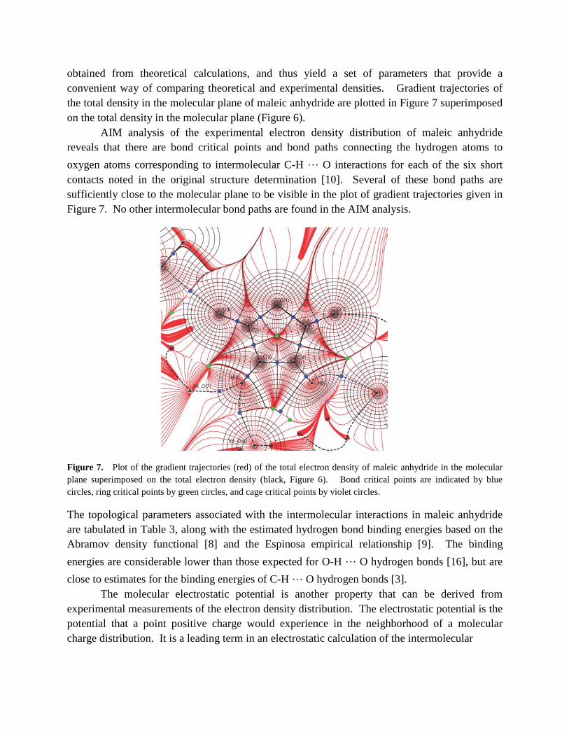
obtained from theoretical calculations, and thus yield a set of parameters that provide a convenient way of comparing theoretical and experimental densities. Gradient trajectories of the total density in the molecular plane of maleic anhydride are plotted in Figure 7 superimposed on the total density in the molecular plane (Figure 6).

AIM analysis of the experimental electron density distribution of maleic anhydride reveals that there are bond critical points and bond paths connecting the hydrogen atoms to oxygen atoms corresponding to intermolecular C-H … O interactions for each of the six short contacts noted in the original structure determination [10]. Several of these bond paths are sufficiently close to the molecular plane to be visible in the plot of gradient trajectories given in Figure 7. No other intermolecular bond paths are found in the AIM analysis.

Figure 7. Plot of the gradient trajectories (red) of the total electron density of maleic anhydride in the molecular plane superimposed on the total electron density (black, Figure 6). Bond critical points are indicated by blue circles, ring critical points by green circles, and cage critical points by violet circles.

The topological parameters associated with the intermolecular interactions in maleic anhydride are tabulated in Table 3, along with the estimated hydrogen bond binding energies based on the Abramov density functional [8] and the Espinosa empirical relationship [9]. The binding energies are considerable lower than those expected for O-H … O hydrogen bonds [16], but are close to estimates for the binding energies of C-H … O hydrogen bonds [3]. The molecular electrostatic potential is another property that can be derived from experimental measurements of the electron density distribution. The electrostatic potential is the potential that a point positive charge would experience in the neighborhood of a molecular charge distribution. It is a leading term in an electrostatic calculation of the intermolecular

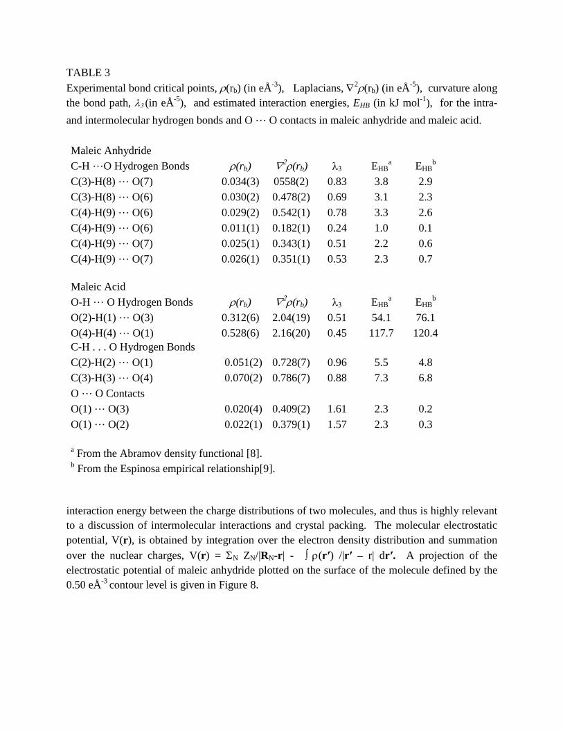
TABLE 3 Experimental bond critical points, ρ(rb) (in eÅ-3), Laplacians, ∇2ρ(rb) (in eÅ-5), curvature along the bond path, λ3 (in eÅ-5), and estimated interaction energies, EHB (in kJ mol-1), for the intra- and intermolecular hydrogen bonds and O … O contacts in maleic anhydride and maleic acid. Maleic Anhydride

C-H …O Hydrogen Bonds ρ(rb) ∇2ρ(rb) λ3 EHBa EHB

b C(3)-H(8) … O(7) 0.034(3) 0558(2) 0.83 3.8 2.9 C(3)-H(8) … O(6) 0.030(2) 0.478(2) 0.69 3.1 2.3 C(4)-H(9) … O(6) 0.029(2) 0.542(1) 0.78 3.3 2.6 C(4)-H(9) … O(6) 0.011(1) 0.182(1) 0.24 1.0 0.1 C(4)-H(9) … O(7) 0.025(1) 0.343(1) 0.51 2.2 0.6 C(4)-H(9) … O(7) 0.026(1) 0.351(1) 0.53 2.3 0.7

Maleic Acid O-H … O Hydrogen Bonds ρ(rb) ∇2ρ(rb) λ3 EHB

a EHBb

O(2)-H(1) … O(3) 0.312(6) 2.04(19) 0.51 54.1 76.1 O(4)-H(4) … O(1) 0.528(6) 2.16(20) 0.45 117.7 120.4 C-H . . . O Hydrogen Bonds

C(2)-H(2) … O(1) 0.051(2) 0.728(7) 0.96 5.5 4.8 C(3)-H(3) … O(4) 0.070(2) 0.786(7) 0.88 7.3 6.8 O … O Contacts

O(1) … O(3) 0.020(4) 0.409(2) 1.61 2.3 0.2 O(1) … O(2) 0.022(1) 0.379(1) 1.57 2.3 0.3

a From the Abramov density functional [8]. b From the Espinosa empirical relationship[9].

interaction energy between the charge distributions of two molecules, and thus is highly relevant to a discussion of intermolecular interactions and crystal packing. The molecular electrostatic potential, V(r), is obtained by integration over the electron density distribution and summation over the nuclear charges, V(r) = ΣN ZN/|RN-r| - ∫ ρ(r′) /|r′ – r| dr′. A projection of the electrostatic potential of maleic anhydride plotted on the surface of the molecule defined by the 0.50 eÅ-3 contour level is given in Figure 8.

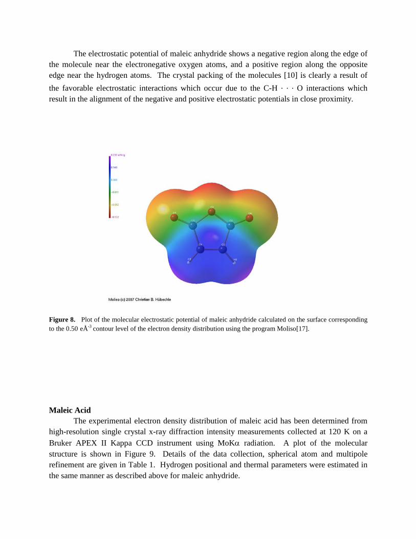
The electrostatic potential of maleic anhydride shows a negative region along the edge of the molecule near the electronegative oxygen atoms, and a positive region along the opposite edge near the hydrogen atoms. The crystal packing of the molecules [10] is clearly a result of the favorable electrostatic interactions which occur due to the C-H . . . O interactions which result in the alignment of the negative and positive electrostatic potentials in close proximity.

Figure 8. Plot of the molecular electrostatic potential of maleic anhydride calculated on the surface corresponding to the 0.50 eÅ-3 contour level of the electron density distribution using the program Moliso[17].

Maleic Acid The experimental electron density distribution of maleic acid has been determined from high-resolution single crystal x-ray diffraction intensity measurements collected at 120 K on a Bruker APEX II Kappa CCD instrument using MoKα radiation. A plot of the molecular structure is shown in Figure 9. Details of the data collection, spherical atom and multipole refinement are given in Table 1. Hydrogen positional and thermal parameters were estimated in the same manner as described above for maleic anhydride.

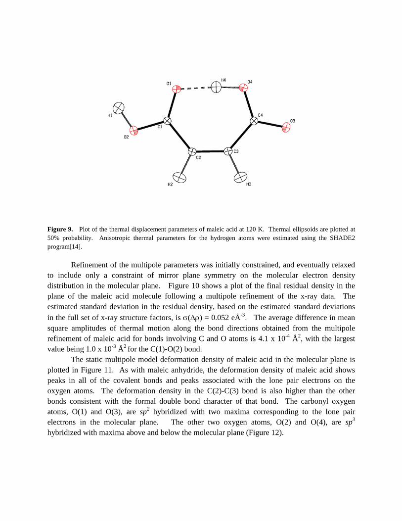
Figure 9. Plot of the thermal displacement parameters of maleic acid at 120 K. Thermal ellipsoids are plotted at 50% probability. Anisotropic thermal parameters for the hydrogen atoms were estimated using the SHADE2 program[14].

Refinement of the multipole parameters was initially constrained, and eventually relaxed to include only a constraint of mirror plane symmetry on the molecular electron density distribution in the molecular plane. Figure 10 shows a plot of the final residual density in the plane of the maleic acid molecule following a multipole refinement of the x-ray data. The estimated standard deviation in the residual density, based on the estimated standard deviations in the full set of x-ray structure factors, is σ(∆ρ) = 0.052 eÅ-3. The average difference in mean square amplitudes of thermal motion along the bond directions obtained from the multipole refinement of maleic acid for bonds involving C and O atoms is 4.1 x 10-4 Å2, with the largest value being 1.0 x 10-3 Å2 for the C(1)-O(2) bond.

The static multipole model deformation density of maleic acid in the molecular plane is plotted in Figure 11. As with maleic anhydride, the deformation density of maleic acid shows peaks in all of the covalent bonds and peaks associated with the lone pair electrons on the oxygen atoms. The deformation density in the C(2)-C(3) bond is also higher than the other bonds consistent with the formal double bond character of that bond. The carbonyl oxygen atoms, O(1) and O(3), are sp2 hybridized with two maxima corresponding to the lone pair electrons in the molecular plane. The other two oxygen atoms, O(2) and O(4), are sp3 hybridized with maxima above and below the molecular plane (Figure 12).

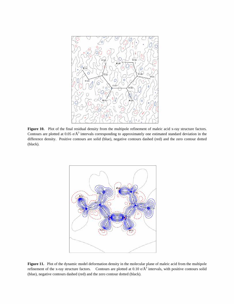
Figure 10. Plot of the final residual density from the multipole refinement of maleic acid x-ray structure factors. Contours are plotted at 0.05 e/Å3 intervals corresponding to approximately one estimated standard deviation in the difference density. Positive contours are solid (blue), negative contours dashed (red) and the zero contour dotted (black).

Figure 11. Plot of the dynamic model deformation density in the molecular plane of maleic acid from the multipole refinement of the x-ray structure factors. Contours are plotted at 0.10 e/Å3 intervals, with positive contours solid (blue), negative contours dashed (red) and the zero contour dotted (black).

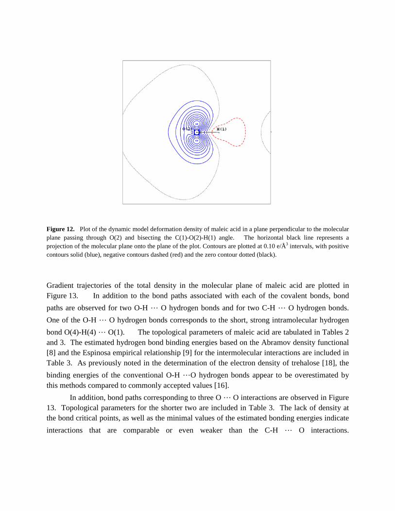
Figure 12. Plot of the dynamic model deformation density of maleic acid in a plane perpendicular to the molecular plane passing through O(2) and bisecting the C(1)-O(2)-H(1) angle. The horizontal black line represents a projection of the molecular plane onto the plane of the plot. Contours are plotted at 0.10 e/Å3 intervals, with positive contours solid (blue), negative contours dashed (red) and the zero contour dotted (black).

Gradient trajectories of the total density in the molecular plane of maleic acid are plotted in Figure 13. In addition to the bond paths associated with each of the covalent bonds, bond paths are observed for two O-H … O hydrogen bonds and for two C-H … O hydrogen bonds. One of the O-H … O hydrogen bonds corresponds to the short, strong intramolecular hydrogen bond O(4)-H(4) … O(1). The topological parameters of maleic acid are tabulated in Tables 2 and 3. The estimated hydrogen bond binding energies based on the Abramov density functional [8] and the Espinosa empirical relationship [9] for the intermolecular interactions are included in Table 3. As previously noted in the determination of the electron density of trehalose [18], the binding energies of the conventional O-H …O hydrogen bonds appear to be overestimated by this methods compared to commonly accepted values [16].

In addition, bond paths corresponding to three O … O interactions are observed in Figure 13. Topological parameters for the shorter two are included in Table 3. The lack of density at the bond critical points, as well as the minimal values of the estimated bonding energies indicate interactions that are comparable or even weaker than the C-H … O interactions.

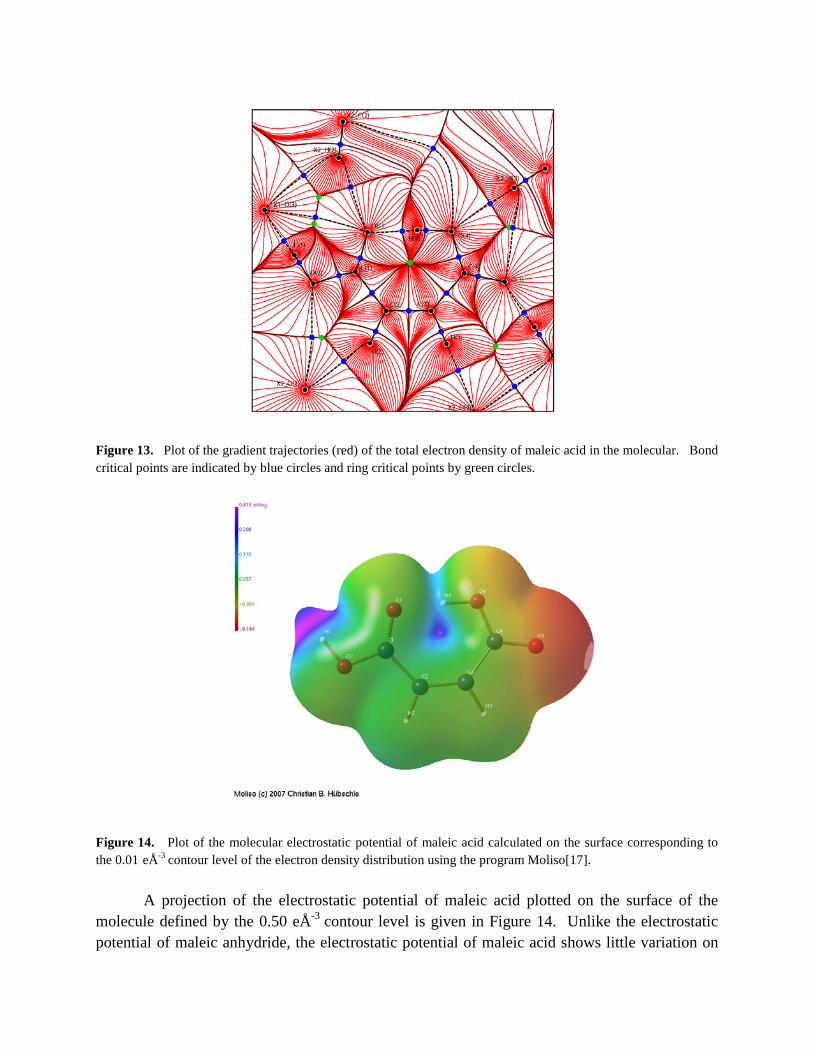
Figure 13. Plot of the gradient trajectories (red) of the total electron density of maleic acid in the molecular. Bond critical points are indicated by blue circles and ring critical points by green circles.

Figure 14. Plot of the molecular electrostatic potential of maleic acid calculated on the surface corresponding to the 0.01 eÅ-3 contour level of the electron density distribution using the program Moliso[17].

A projection of the electrostatic potential of maleic acid plotted on the surface of the molecule defined by the 0.50 eÅ-3 contour level is given in Figure 14. Unlike the electrostatic potential of maleic anhydride, the electrostatic potential of maleic acid shows little variation on

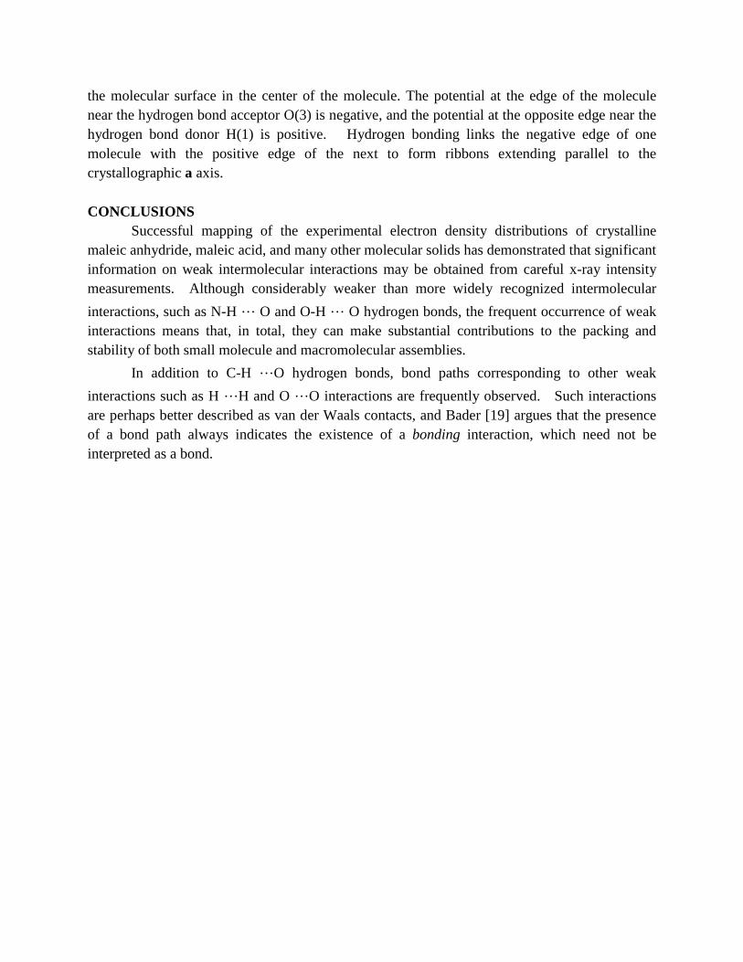
the molecular surface in the center of the molecule. The potential at the edge of the molecule near the hydrogen bond acceptor O(3) is negative, and the potential at the opposite edge near the hydrogen bond donor H(1) is positive. Hydrogen bonding links the negative edge of one molecule with the positive edge of the next to form ribbons extending parallel to the crystallographic a axis. CONCLUSIONS Successful mapping of the experimental electron density distributions of crystalline maleic anhydride, maleic acid, and many other molecular solids has demonstrated that significant information on weak intermolecular interactions may be obtained from careful x-ray intensity measurements. Although considerably weaker than more widely recognized intermolecular interactions, such as N-H … O and O-H … O hydrogen bonds, the frequent occurrence of weak interactions means that, in total, they can make substantial contributions to the packing and stability of both small molecule and macromolecular assemblies.

In addition to C-H …O hydrogen bonds, bond paths corresponding to other weak interactions such as H …H and O …O interactions are frequently observed. Such interactions are perhaps better described as van der Waals contacts, and Bader [19] argues that the presence of a bond path always indicates the existence of a bonding interaction, which need not be interpreted as a bond.

ACKNOWLEDGMENTS Support of this research from Louisiana Board of Regents Grant No. LEQSF(2007-12)-

ENH-PKSFI-PRS-04 is gratefully acknowledged. REFERENCES [1] T. S. Koritsánszky and P. Coppens, Chem. Rev. 101(2001), 1583−1627. [2] P. Coppens, X-ray Charge Densities and Chemical Bonding, (Oxford University Press, New York, 1997). [3] T. Steiner, Crystallogr. Rev. 5 (1996), 1-57. [4] M. J. Frisch, et al., Gaussian 03, Revision C.02 (Wallingford CT, 2004). [5] R. W. F. Bader, Atoms in Molecules: a Quantum Theory, (Clarendon Press, Oxford, 1990). [6] N. K. Hansen and P. Coppens, Acta Crystallogr. Sect. A34, (1978) 909−921. [7] A. Volkov, P. Macchi, L. J. Farrugia, C. Gatti, P. Mallinson, T. Richter, and T. Koritsanszky, XD2006 - A Computer Program for Multipole Refinement, Topological Analysis of Charge Densities and Evaluation of Intermolecular Energies from Experimental or Theoretical Structure Factors (Middle Tennessee State University, 2006). [8] Y. A. Abramov, Acta Crystallogr. Sect. A 53 (1997), 264−272. [9] E. Espinosa, E. Molins, and C. Lecomte, Chem. Phys. Lett. 258(1998), 170−173 [10] R. E. Marsh, E. Ubell, and H. E. Wilcox, Acta Crystallogr. 15(1962), 35-41. [11] M. N. G. James and G. J. B. Williams, Acta Crystallogr. Sect. B 30(1974),1249-1257. [12] L. Huang, L. Massa, and J. Karle, J. Quantum Chem. 73(1999), 439-450. [13] F. H. Allen and I. J. Bruno, Acta Crystallogr. Sect. B 66(2010), 380-386. [14] P. Munshi, A. Ø. Madsen, M. A. Spackman, S. Larsen and R. Destro, Acta Crystallogr. Sect. A 64(2008)465-475. [15] F. L. Hirshfeld, Acta Crystallogr., Sect. A 30 (1976), 239−244. [16] G. A. Jeffrey and W. Saenger, Hydrogen Bonding in Biological Structures, (Springer- Verlag, New York, (1991 [17] C. B. Hübschle and P. Luger, J. Appl. Crystallogr. 39 (2006), 901−904. [18] E. D. Stevens, M. K. Dowd, G. P. Johnson, and A. D. French, Carbohydr. Res. 345 (2010), 1469-1481. [19] R. W. F. Bader, J. Phys. Chem. A 113, (2009), 10391-10396.