8.5 absolute convergence and the ratio … chapter 8 inﬁnite series 8.5 absolute convergence and...

666 Chapter 8 Infinite Series

8.5 ABSOLUTE CONVERGENCE AND THE RATIO TEST

You should note that, outside of the Alternating Series Test presented in section 8.4, ourother tests for convergence of series (i.e., the Integral Test and the two comparison tests)apply only to series all of whose terms are positive. So, what do we do if we’re faced witha series that has both positive and negative terms, but that is not an alternating series? Forinstance, look at the series

∞∑k=1

sin k

k3= sin 1 + 1

8sin 2 + 1

27sin 3 + 1

64sin 4 + · · · .

This has both positive and negative terms, but the terms do not alternate signs. (Calculate

the first five or six terms of the series to see this for yourself.) For any such series ∞∑

k=1ak,

we can get around this problem by checking if the series of absolute values ∞∑

k=1|ak | is con-

vergent. When this happens, we say that the original series ∞∑

k=1ak is absolutely convergent

(or converges absolutely). You should note that to test the convergence of the series of

absolute values ∞∑

k=1|ak | (all of whose terms are positive), we have all of our earlier tests

for positive term series available to us.

Determine if ∞∑

k=1

(−1)k+1

2kis absolutely convergent.

Solution It is easy to show that this alternating series is convergent. (Try it!)From the graph of the first 20 partial sums in Figure 8.34, it appears that the seriesconverges to approximately 0.35. To determine absolute convergence, we need to

determine whether or not the series of absolute values, ∞∑

k=1

∣∣∣∣ (−1)k+1

2k

∣∣∣∣ is convergent. Wehave

∞∑k=1

∣∣∣∣ (−1)k+1

2k

∣∣∣∣ =∞∑

k=1

1

2k=

∞∑k=1

(1

2

)k

,

which you should recognize as a convergent geometric series (|r | = 12 < 1). This says

that the original series ∞∑

k=1

(−1)k+1

2kconverges absolutely.

■

You might be wondering what the relationship is between convergence and absoluteconvergence. We’ll prove shortly that every absolutely convergent series is also conver-gent (as in example 5.1). However, the reverse is not true; there are many series that areconvergent, but not absolutely convergent. These are called conditionally convergentseries. Can you think of an example of such a series? If so, it’s probably the example thatfollows.

Testing for Absolute ConvergenceExample 5.1

5 10 15 20

0.1

0.2

0.3

0.4

0.5

Sn

n

Figure 8.34

Sn =n∑

k=1

(−1)k+1

2k.

smi98485_ch08b.qxd 5/17/01 2:07 PM Page 666

Determine if the alternating harmonic series ∞∑

k=1

(−1)k+1

kis absolutely convergent.

Solution In example 4.2, we showed that this series is convergent. To test this forabsolute convergence, we consider the series of absolute values,

∞∑k=1

∣∣∣∣ (−1)k+1

k

∣∣∣∣ =∞∑

k=1

1

k,

which is the harmonic series. We showed in section 8.2 (example 2.7) that the harmonic

series diverges. This says that ∞∑

k=1

(−1)k+1

kconverges, but does not converge absolutely

(i.e., it converges conditionally).

■

This result says that if a series converges absolutely, then it must also converge.Because of this, when we test series, we first test for absolute convergence. If the seriesconverges absolutely, then we need not test any further to establish convergence.

Notice that for any real number, x,we can say that −|x | ≤ x ≤ |x |. So, for any k,we have

−|ak | ≤ ak ≤ |ak |.Adding |ak | to all the terms, we get

0 ≤ ak + |ak | ≤ 2|ak |. (5.1)

Since ∞∑

k=1ak is absolutely convergent, we have that

∞∑k=1

|ak | and hence, also ∞∑

k=12|ak | =

2∞∑

k=1|ak | is convergent. Define bk = ak + |ak |. From (5.1),

0 ≤ bk ≤ 2|ak |and so, by the Comparison Test,

∞∑k=1

bk is convergent. Observe that we may write

∞∑k=1

ak =∞∑

k=1

(ak + |ak | − |ak |) =∞∑

k=1

(ak + |ak |)︸︷︷︸ −∞∑

k=1

|ak |bk

=∞∑

k=1

bk −∞∑

k=1

|ak |.

Since the two series on the right-hand side are convergent, it follows that ∞∑

k=1ak must

also be convergent.

■

Proof

Theorem 5.1

If ∞∑

k=1|ak | converges, then

∞∑k=1

ak converges.

A Conditionally Convergent SeriesExample 5.2

Section 8.5 Absolute Convergence and the Ratio Test 667


Determine whether ∞∑

k=1

sin k

k3is convergent or divergent.

Solution Notice that while this is not a positive term series, it is also not an alter-nating series. Because of this, our only choice (given what we know) is to test the seriesfor absolute convergence. From the graph of the first 20 partial sums seen in Fig-ure 8.35, it appears that the series is converging to some value around 0.94. To test for

absolute convergence, we consider the series of absolute values, ∞∑

k=1

∣∣∣∣ sin k

k3

∣∣∣∣ . Notice that

∣∣∣∣ sin k

k3

∣∣∣∣ = | sin k|k3

≤ 1

k3, (5.2)

since |sin k| ≤ 1, for all k. Of course, ∞∑

k=1

1

k3is a convergent p-series (p = 3 > 1). By

the Comparison Test and (5.2), ∞∑

k=1

∣∣∣∣ sin k

k3

∣∣∣∣ converges, too. Consequently, the original

series ∞∑

k=1

sin k

k3converges absolutely (and hence, converges).

■

The Ratio TestWe now introduce a very powerful tool for testing a series for absolute convergence. Thistest can be applied to a wide range of series, including the extremely important case of powerseries that we discuss in section 8.6. As you’ll see, this test is also remarkably easy to use.

(i) For L < 1, pick any number r with L < r < 1. Then, we have

limk→∞

∣∣∣∣ak+1

ak

∣∣∣∣ = L < r.

For this to occur, there must be some number N > 0, such that for k ≥ N ,∣∣∣∣ak+1

ak

∣∣∣∣ < r. (5.3)

Proof

Theorem 5.2 (Ratio Test)

Given ∞∑

k=1ak , with ak �= 0 for all k, suppose that

limk→∞

∣∣∣∣ak+1

ak

∣∣∣∣ = L .

Then,(i) if L < 1, the series converges absolutely,

(ii) if L > 1 (or L = ∞), the series diverges and(iii) if L = 1, there is no conclusion.

Testing for Absolute ConvergenceExample 5.3


5 10 15 20

0.86

0.90

0.94

0.98

Sn

n

Figure 8.35

Sn =n∑

k=1

sin k

k3.


Multiplying both sides of (5.3) by |ak | gives us

|ak+1| < r |ak |.In particular, taking k = N gives us

|aN+1| < r |aN |and taking k = N + 1 gives us

|aN+2| < r |aN+1| < r2|aN |.Likewise,

|aN+3| < r |aN+2| < r3|aN |and so on. We have

|aN+k | < rk |aN |, for k = 1, 2, 3, . . . .

Notice that ∞∑

k=1|aN | rk = |aN |

∞∑k=1

rk is a convergent geometric series, since 0 < r < 1.

By the Comparison Test, it follows that ∞∑

k=1|aN+k | =

∞∑n=N+1

|an| converges, too. This

says that ∞∑

n=N+1an converges absolutely. Finally, since

∞∑n=1

an =N∑

n=1

an +∞∑

n=N+1

an,

we also get that ∞∑

n=1an converges absolutely.

(ii) For L > 1, we have

limk→∞

∣∣∣∣ak+1

ak

∣∣∣∣ = L > 1.

This says that there must be some number N > 0, such that for k ≥ N , ∣∣∣∣ak+1

ak

∣∣∣∣ > 1. (5.4)

Multiplying both sides of (5.4) by |ak |, we get

|ak+1| > |ak | > 0, for all k ≥ N .

Notice that if this is the case, then

limk→∞

ak �= 0.

By the kth-term test for divergence, we now have that ∞∑

k=1ak diverges.

■

Test ∞∑

k=1

(−1)kk

2kfor convergence.

Solution From the graph of the first 20 partial sums of the series of absolute

values,∞∑

k=1

k

2k, seen in Figure 8.36, it appears that the series of absolute values converges

Using the Ratio TestExample 5.4


5 10 15 20

1.0

1.5

2.0

0.5

Sn

n

Figure 8.36

Sn =n∑

k=1

k

2k.


to about 2. From the Ratio Test, we have

limk→∞

∣∣∣∣ak+1

ak

∣∣∣∣ = limk→∞

k + 1

2k+1

k

2k

= limk→∞

k + 1

2k+1

2k

k= 1

2lim

k→∞k + 1

k= 1

2< 1

and so, the series converges absolutely, as expected from Figure 8.36.

■

The Ratio Test is particularly useful when the general term of a series contains anexponential term, as in example 5.4 or a factorial, as in the following example.

Test ∞∑

k=0

(−1)kk!

ekfor convergence.

Solution From the graph of the first 20 partial sums of the series seen in Fig-ure 8.37, it appears that the series is diverging. (Look closely at the scale on the y-axisand compute a table of values for yourself.) We can confirm this suspicion with theRatio Test. We have

limk→∞

∣∣∣∣ak+1

ak

∣∣∣∣ = limk→∞

(k + 1)!

ek+1

k!

ek

= limk→∞

(k + 1)!

ek+1

ek

k!

= limk→∞

(k + 1) k!

e k!= 1

elim

k→∞k + 1

1= ∞.

By the Ratio Test, the series diverges, as we suspected.

■

Recall that in the statement of the Ratio Test (Theorem 5.2), we said that if

limk→∞

∣∣∣∣ak+1

ak

∣∣∣∣ = 1,

then the Ratio Test yields no conclusion. By this, we mean that in such cases, the series mayor may not converge and further testing is required.

Use the Ratio Test for the harmonic series ∞∑

k=0

1

k.

Solution We have

limk→∞

∣∣∣∣ak+1

ak

∣∣∣∣ = limk→∞

1

k + 11

k

= limk→∞

k

k + 1= 1.

In this case, the Ratio Test yields no conclusion, although we already know that theharmonic series diverges.

■

A Divergent Series for Which the Ratio Test FailsExample 5.6

Since (k + 1)! = (k + 1) · k!

and ek+1 = ek · e1.

Using the Ratio TestExample 5.5

Since

2k+1 = 2k · 21.


5 10 15 20

�4 � 108

�6 � 108

�2 � 108

2 � 108

Sn

n

Figure 8.37

Sn =n−1∑k=0

(−1)k k!

ek.

H I S T O R I C A L N O T E S

Srinivasa Ramanujan(1887–1920) Indianmathematician whose incrediblediscoveries about infinite series stillmystify mathematicians. Largelyself-taught, Ramanujan fillednotebooks with conjectures aboutseries, continued fractions and theRiemann zeta function. Ramanujanrarely gave a proof or evenjustification of his results.Nevertheless, the famous Englishmathematician G. H. Hardy said,“They must be true because, if theyweren’t true, no one would havehad the imagination to inventthem.” (See Exercise 43.)


Use the Ratio Test to test the series ∞∑

k=0

1

k2.

Solution Here, we have

limk→∞

∣∣∣∣ak+1

ak

∣∣∣∣ = limk→∞

1

(k + 1)2

k2

1

= limk→∞

k2

k2 + 2k + 1= 1.

So again, the Ratio Test yields no conclusion, although we already know that this is aconvergent p-series.

■

Look carefully at examples 5.6 and 5.7. You should recognize that the Ratio Test willbe inconclusive for any p-series. Of course, we don’t need the Ratio Test for these series.

We now present one final test for convergence of series.

Notice how similar the conclusion is to the conclusion of the Ratio Test. The proof isalso similar to that of the Ratio Test and we leave this as an exercise.

Use the Root Test to determine the convergence or divergence of the series ∞∑

k=1

(2k + 4

5k − 1

)k

.

Solution In this case, we consider

limk→∞

k√

|ak | = limk→∞

k

√∣∣∣∣2k + 4

5k − 1

∣∣∣∣k

= limk→∞

2k + 4

5k − 1= 2

5< 1.

By the Root Test, the series is absolutely convergent.

■

By this point in your study of series, it may seem as if we have thrown at you a dizzy-ing array of different series and tests for convergence or divergence. Just how are you tokeep all of these straight? The only suggestion we have is that you work through manyproblems. We provide a good assortment in the exercise set that follows this section. Some

Using the Root TestExample 5.8

Theorem 5.3 (Root Test)

Given ∞∑

k=1ak, suppose that lim

k→∞k√

|ak | = L . Then,

(i) if L < 1, the series converges absolutely,(ii) if L > 1 (or L = ∞), the series diverges and

(iii) if L = 1, there is no conclusion.

A Convergent Series for Which the Ratio Test FailsExample 5.7


smi98485_ch08b.qxd 5/17/01 2:07 PM 71

of these require the methods of this section, while others are drawn from the preceding sec-tions ( just to keep you thinking about the big picture). For the sake of convenience, wesummarize our convergence tests in the table that follows.


Test When to use Conclusions Section

Geometric Series∞∑

k=0ark Converges to

a

1 − rif |r | < 1; 8.2

diverges if |r | ≥ 1.

kth Term Test All series If limk→∞

ak �= 0, the series diverges. 8.2

Integral Test∞∑

k=1ak where f (k) = ak and

∞∑k=1

ak and ∫ ∞

1f (x) dx 8.3

f is continuous, decreasing and f (x) ≥ 0 both converge or both diverge.

p-series∞∑

k=1

1

k pConverges for p > 1; diverges for p ≤ 1. 8.3

Comparison Test∞∑

k=1ak and

∞∑k=1

bk , where 0 ≤ ak ≤ bk If ∞∑

k=1bk converges, then

∞∑k=1

ak converges. 8.3

If ∞∑

k=1ak diverges, then

∞∑k=1

bk diverges.

Limit Comparison Test∞∑

k=1ak and

∞∑k=1

bk , where∞∑

k=1ak and

∞∑k=1

bk 8.3

ak , bk > 0 and limk→∞

ak

bk= L > 0 both converge or both diverge.

Alternating Series Test∞∑

k=1(−1)k+1ak where ak > 0 for all k If lim

k→∞ak = 0 and ak+1 ≤ ak for all k, 8.4

then the series converges.

Absolute Convergence Series with some positive and some If ∞∑

k=1|ak | converges, then 8.5

negative terms (including alternating series)∞∑

k=1ak converges (absolutely).

Ratio Test Any series (especially those involving For limk→∞

∣∣∣∣ak+1

ak

∣∣∣∣ = L , 8.5 exponentials and/or factorials)

if L < 1,∞∑

k=1ak converges absolutely

if L > 1,∞∑

k=1ak diverges,

if L = 1, no conclusion.

Root Test Any series (especially those involving For limk→∞

k√

|ak | = L , 8.5exponentials)

if L < 1,∞∑

k=1ak converges absolutely

if L > 1,∞∑

k=1ak diverges,

if L = 1, no conclusion.


EXERCISES 8.5


1. Suppose that two series have identical terms except thatin series A all terms are positive and in series B some

terms are positive and some terms are negative. Explain whyseries B is more likely to converge. In light of this, explain whyTheorem 5.1 is true.

2. In the Ratio Test, if limk→∞

∣∣∣∣ak+1

ak

∣∣∣∣ > 1, which is bigger,

|ak+1| or |ak |? Explain why this implies that the series∞∑

k=1ak diverges.

3. In the Ratio Test, if limk→∞

∣∣∣∣ak+1

ak

∣∣∣∣ = L < 1, which is

bigger, |ak+1| or |ak |? This inequality could also hold ifL = 1. Compare the relative sizes of |ak+1| and |ak | if L = 0.8versus L = 1. Explain why L = 0.8 would be more likely tocorrespond to a convergent series than L = 1.

4. In many series of interest, the terms of the series involvepowers of k (e.g., k2), exponentials (e.g., 2k ) or factori-

als (e.g., k!). For which type(s) of terms is the Ratio Test likelyto produce a result (i.e., a limit different than 1)? Brieflyexplain.

In exercises 5–42, determine if the series is absolutely conver-gent, conditionally convergent or divergent.

5.∞∑

k=0

(−1)k 3

k!6.

∞∑k=0

(−1)k 6

k!

7.∞∑

k=0

(−1)k 2k 8.∞∑

k=0

(−1)k 2

3k

9.∞∑

k=1

(−1)k+1 k

k2 + 110.

∞∑k=1

(−1)k+1 k2 + 1

k

11.∞∑

k=0

(−1)k 3k

k!12.

∞∑k=0

(−1)k 10k

k!

13.∞∑

k=1

(−1)k+1 k

2k + 114.

∞∑k=1

(−1)k+1 4

2k + 1

15.∞∑

k=1

(−1)k k2k

3k16.

∞∑k=1

(−1)k k23k

2k

17.∞∑

k=1

(4k

5k + 1

)k

18.∞∑

k=1

(1 − 3k

4k

)k

19.∞∑

k=1

−2

k20.

∞∑k=1

4

k

21.∞∑

k=1

(−1)k+1

√k

k + 122.

∞∑k=1

(−1)k+1 k

k3 + 1

23.∞∑

k=1

k2

ek24.

∞∑k=1

k3e−k

25.∞∑

k=2

e3k

k3k26.

∞∑k=1

(ek

k2

)k

27.∞∑

k=1

sin k

k228.

∞∑k=1

cos k

k3

29.∞∑

k=1

cos kπ

k30.

∞∑k=1

sin kπ

k

31.∞∑

k=2

(−1)k

ln k32.

∞∑k=2

(−1)k

k ln k

33.∞∑

k=1

(−1)k

k√

k34.

∞∑k=1

(−1)k+1

√k

35.∞∑

k=1

3

kk36.

∞∑k=0

2k

3k

37.∞∑

k=1

(−1)k+1 k!

4k38.

∞∑k=1

(−1)k+1 k24k

k!

39.∞∑

k=1

(−1)k+1 k10

(2k)!40.

∞∑k=0

(−1)k 4k

(2k + 1)!

41.∞∑

k=0

(−2)k (k + 1)

5k42.

∞∑k=1

(−3)k

k24k

43. In the 1910s, the Indian mathematician Srinivasa Ramanujandiscovered the formula

1

π=

√8

9801

∞∑k=0

(4k)!(1103 + 26,390k)

(k!)43964k.

Approximate the series with only the k = 0 term and show thatyou get 6 digits of π correct. Approximate the series using thek = 0 and k = 1 terms and show that you get 14 digits of πcorrect. In general, each term of this remarkable series in-creases the accuracy by 8 digits.



44. Prove that Ramanujan’s series in exercise 43 converges.

45. To show that ∞∑

k=1

k!

kkconverges, use the Ratio Test and the fact

that

limk→∞

(k + 1

k

)k

= limk→∞

(1 + 1

k

)k

= e.

46. Determine whether ∞∑

k=1

k!

1 · 3 · 5 · · · (2k − 1)converges or

diverges.

47. One reason that it is important to distinguish absolutefrom conditional convergence of a series is the rearrange-

ment of series, to be explored in this exercise. Show that the

series ∞∑

k=0

(−1)k

2kis absolutely convergent and find its sum S.

Find the sum S+ of the positive terms of the series. Find thesum S− of the negative terms of the series. Verify thatS = S+ + S− . This may seem obvious, since for the finitesums you are most familiar with, the order of addition nevermatters. However, you cannot separate the positive and nega-tive terms for conditionally convergent series. For example,

show that ∞∑

k=0

(−1)k

k + 1converges (conditionally) but that the

series of positive terms and the series of negative terms bothdiverge. Explain in words why this will always happen forconditionally convergent series. Thus, the order of terms mat-ters for conditionally convergent series. By exploring further,we can uncover a truly remarkable fact: for conditionally con-vergent series, you can reorder the terms so that the partialsums converge to any real number. To illustrate this, suppose

we want to reorder the series ∞∑

k=0

(−1)k

k + 1so that the partial sums

converge to π

2 . Start by pulling out positive terms(1 + 1

3 + 15 + · · ·) such that the partial sum is within 0.1 of π

2 .Next, take the first negative term

(− 12

)and positive terms such

that the partial sum is within 0.05 of π

2 . Then take the nextnegative term

(− 14

)and positive terms such that the partial sum

is within 0.01 of π

2 . Argue that you could continue in thisfashion to reorder the terms so that the partial sums converge toπ

2 . (Especially explain why you will never “run out of’’ posi-tive terms.) Then explain why you cannot do the same with the

absolutely convergent series ∞∑

k=0

(−1)k

2k.

8.6 POWER SERIES

We now want to expand our discussion of series to the case where the terms of the seriesare functions of the variable x . Pay close attention to what we are about to introduce, forthis is the culmination of all your hard work in the preceding five sections. The primaryreason for studying series is that we can use them to represent functions. This opens upall kinds of possibilities for us, from approximating the values of transcendental functionsto calculating derivatives and integrals of such functions, to studying differential equa-tions. As well, defining functions as convergent series produces an explosion of newfunctions available to us. In fact, many functions of great significance in applications (forinstance, Bessel functions) are defined as a series. We take the first few steps in thissection.

As a start, consider the series

∞∑k=0

(x − 2)k = 1 + (x − 2) + (x − 2)2 + (x − 2)3 + · · · .

Notice that for each fixed x, this is a geometric series with r = (x − 2). Recall that thissays that the series will converge whenever |r | = |x − 2| < 1 and will diverge whenever|r | = |x − 2| ≥ 1. Further, for each x with |x − 2| < 1 (i.e., 1 < x < 3), the series con-verges to

a

1 − r= 1

1 − (x − 2)= 1

3 − x.


That is, for each x in the interval (1, 3), we have

∞∑k=0

(x − 2)k = 1

3 − x.

For all other values of x, the series diverges. In Figure 8.38, we show a graph of f (x) =1

3 − x, along with the first three partial sums Pn, of this series, where

Pn(x) =n∑

k=0

(x − 2)k = 1 + (x − 2) + (x − 2)2 + · · · + (x − 2)n,

on the interval [1, 3]. Notice that as n gets larger, Pn(x) appears to get closer to f (x), forany given x in the interval (1, 3). Further, as n gets larger, Pn(x) tends to stay close to f (x)

for a larger range of x-values.Make certain that you understand what we’ve observed here: we have taken a se-

ries and noticed that it is equivalent to (i.e., it converges to) a known function on a cer-tain interval. You might ask why anyone would care if you could do that. Certainly,

f (x) = 1

3 − xis a perfectly good function and anything you’d want to do with it will most

definitely be easier using the algebraic expression 1

3 − xthan using the equivalent series

representation, ∞∑

k=0(x − 2)k . However, imagine what benefits you might find if you could

take a given function (say, one that you don’t know a whole lot about) and find an equiva-lent series representation. This is precisely what we are going to do in section 8.7. Forinstance, we will be able to show that for all x,

ex =∞∑

k=0

xk

k!= 1 + x + x2

2!+ x3

3!+ x4

4!+ · · · . (6.1)

So, who cares? Well, suppose you wanted to calculate e1.234567. How would you do that?Of course, you’d use a calculator. But, haven’t you ever wondered how your calculatordoes it? The problem is that ex is not an algebraic function. That is, we can’t compute itsvalues by using algebraic operations (i.e., addition, subtraction, multiplication, divisionand nth roots). Over the next few sections, we begin to explore this question. For the mo-ment, let us say this: if we have the series representation (6.1) for ex , then for any given x ,we can compute an approximation to ex , simply by summing the first few terms of theequivalent power series. This is easy to do, since the partial sums of the series are simplypolynomials.

In general, any series of the form

∞∑k=0

bk(x − c)k = b0 + b1(x − c) + b2(x − c)2 + b3(x − c)3 + · · ·

is called a power series in powers of (x − c). We refer to the constants bk, k = 0, 1, 2, . . .

as the coefficients of the series. The first question is: for what values of x does the series

converge? Saying this another way, the power series ∞∑

k=0bk(x − c)k defines a function of x .

Its domain is the set of all x for which the series converges. The primary tool for inves-tigating the convergence or divergence of a power series is the Ratio Test. Notice againthat the partial sums of a power series are all polynomials (the simplest functionsaround).

Section 8.6 Power Series 675

321

�1

1

2

3 y � f (x)

y � P1(x)

y � P2(x)

y � P3(x)

y

x

Figure 8.38

y = 1

3 − xand the first three partial

sums of ∞∑

k=0(x − 2)k .

Power series


Determine the values of x for which the power series ∞∑

k=0

k

3k+1xk converges.

Solution Using the Ratio Test, we have

limk→∞

∣∣∣∣ak+1

ak

∣∣∣∣ = limk→∞

∣∣∣∣ (k + 1)xk+1

3k+2

3k+1

kxk

∣∣∣∣= lim

k→∞(k + 1)|x |

3k= |x |

3lim

k→∞k + 1

k

= |x |3

< 1,

for |x | < 3 or −3 < x < 3. So, the series converges absolutely for −3 < x < 3 anddiverges for |x | > 3 (i.e., for x > 3 or x < −3). Since the Ratio Test gives no conclu-sion for the endpoints x = ±3, we must test these separately.

For x = 3, we have the series∞∑

k=0

k

3k+1xk =

∞∑k=0

k

3k+13k =

∞∑k=0

k

3.

Since

limk→∞

k

3= ∞ �= 0,

the series diverges by the kth-term test for divergence. The series diverges when x = −3,

for the same reason. Thus, the power series converges for all x in the interval (−3, 3)

and diverges for all x outside this interval.

■

Observe that example 6.1 has something in common with the introductory example. In

both cases, the series have the form ∞∑

k=0bk(x − c)k and there is an interval of the form

(c − r, c + r) on which the series converges and outside of which the series diverges. (Inthe case of example 6.1, notice that c = 0.) This interval on which a power series convergesis called the interval of convergence. The constant r is called the radius of convergence(i.e., r is half the length of the interval of convergence). It turns out that there is such aninterval for every power series. We have the following result.

The proof of the theorem can be found in Appendix A.

Theorem 6.1

Given any power series, ∞∑

k=0bk(x − c)k, there are exactly three possibilities:

(i) The series converges for all x ∈ (−∞,∞) and the radius of convergence isr = ∞;

(ii) The series converges only for x = c (and diverges for all other values of x) andthe radius of convergence is r = 0; or

(iii) The series converges for x ∈ (c − r, c + r) and diverges for x < c − r and forx > c + r , for some number r with 0 < r < ∞.

Since xk+1 = xk · x1

and 3k+2 = 3k+1 · 31.

Determining Where a Power Series ConvergesExample 6.1



Determine the interval and radius of convergence for the power series ∞∑

k=0

10k

k!(x − 1)k .

Solution From the Ratio Test, we have

limk→∞

∣∣∣∣ak+1

ak

∣∣∣∣ = limk→∞

∣∣∣∣10k+1(x − 1)k+1

(k + 1)!

k!

10k(x − 1)k

∣∣∣∣= 10|x − 1| lim

k→∞k!

(k + 1)k!

= 10|x − 1| limk→∞

1

k + 1= 0 < 1,

for all x . This says that the series converges absolutely for all x . Thus, the interval ofconvergence for this series is (−∞,∞) and the radius of convergence is r = ∞.

■

The interval of convergence for a power series can be a closed interval, an open inter-val or a half-open interval, as in the following example.

Determine the interval and radius of convergence for the power series ∞∑

k=1

xk

k 4k.


limk→∞

∣∣∣∣ak+1

ak

∣∣∣∣ = limk→∞

∣∣∣∣ xk+1

(k + 1)4k+1

k 4k

xk

∣∣∣∣= |x |

4lim

k→∞k

k + 1= |x |

4< 1.

So, we are guaranteed absolute convergence for |x | < 4 and divergence for |x | > 4. Itremains only to test the endpoints of the interval: x = ±4. For x = 4, we have

∞∑k=1

xk

k 4k=

∞∑k=1

4k

k 4k=

∞∑k=1

1

k,

which you will recognize as the harmonic series, which diverges. For x = −4, we have∞∑

k=1

xk

k 4k=

∞∑k=1

(−4)k

k 4k=

∞∑k=1

(−1)k

k,

which is the alternating harmonic series, which we know converges (see example 4.2).So, in this case, the interval of convergence is the half-open interval [−4, 4) and theradius of convergence is r = 4.

■

Notice that (as stated in Theorem 6.1) every power series, ∞∑

k=0ak(x − c)k converges at

least for x = c since for x = c, we have the trivial case ∞∑

k=0

ak(x − c)k =∞∑

k=0

ak(c − c)k = a0 +∞∑

k=1

ak0k = a0 + 0 = a0.

A Half-Open Interval of ConvergenceExample 6.3

Since (x − 1)k+1 = (x − 1)k(x − 1)1

and (k + 1)! = (k + 1)k!

Finding the Interval and Radius of ConvergenceExample 6.2



Determine the radius of convergence for the power series ∞∑

k=0k!(x − 5)k .


limk→∞

∣∣∣∣ak+1

ak

∣∣∣∣ = limk→∞

∣∣∣∣ (k + 1)!(x − 5)k+1

k!(x − 5)k

∣∣∣∣= lim

k→∞(k + 1)k!|x − 5|

k!

= limk→∞

[(k + 1)|x − 5|]

={

0, if x = 5∞, if x �= 5

.

Thus, this power series converges only for x = 5 and so, its radius of convergence isr = 0.

■

Suppose that the power series ∞∑

k=0bk(x − c)k has radius of convergence r > 0. Then

the series converges absolutely for all x in the interval (c − r, c + r) and might convergeat one or both of the endpoints, x = c − r and x = c + r . Notice that since the series con-verges for each x ∈ (c − r, c + r), it defines a function f on the interval (c − r, c + r),

f (x) =∞∑

k=0

bk(x − c)k = b0 + b1(x − c) + b2(x − c)2 + b3(x − c)3 + · · · .

It turns out that such a function is continuous and differentiable, although the proof is be-yond the level of this course. In fact, we differentiate exactly the way you might expect,

f ′(x) = d

dxf (x) = d

dx[b0 + b1(x − c) + b2(x − c)2 + b3(x − c)3 + · · ·]

= b1 + 2b2(x − c) + 3b3(x − c)2 + · · · =∞∑

k=1

bkk(x − c)k−1,

where the radius of convergence of the resulting series is also r. Since we find the deriva-tive by differentiating each term in the series, we call this term-by-term differentiation.Likewise, we can integrate a convergent power series term-by-term,∫

f (x)dx =∫ ∞∑

k=0

bk(x − c)k dx =∞∑

k=0

bk

∫(x − c)k dx

=∞∑

k=0

bk(x − c)k+1

k + 1+ K ,

where the radius of convergence of the resulting series is again r and where K is a constantof integration. The proof of these two results can be found in a text on advanced calculus.It’s important to recognize that these two results are not obvious. They are not simply anapplication of the rule that a derivative or integral of a sum is simply the sum of the deriv-atives or integrals, respectively, since a series is not a sum, but rather, a limit of a sum.(What’s the difference, anyway?) Further, these results are true for power series, but arenot true for series in general.

A Power Series That Converges at Only One PointExample 6.4


Differentiating a power series

Integrating a power series


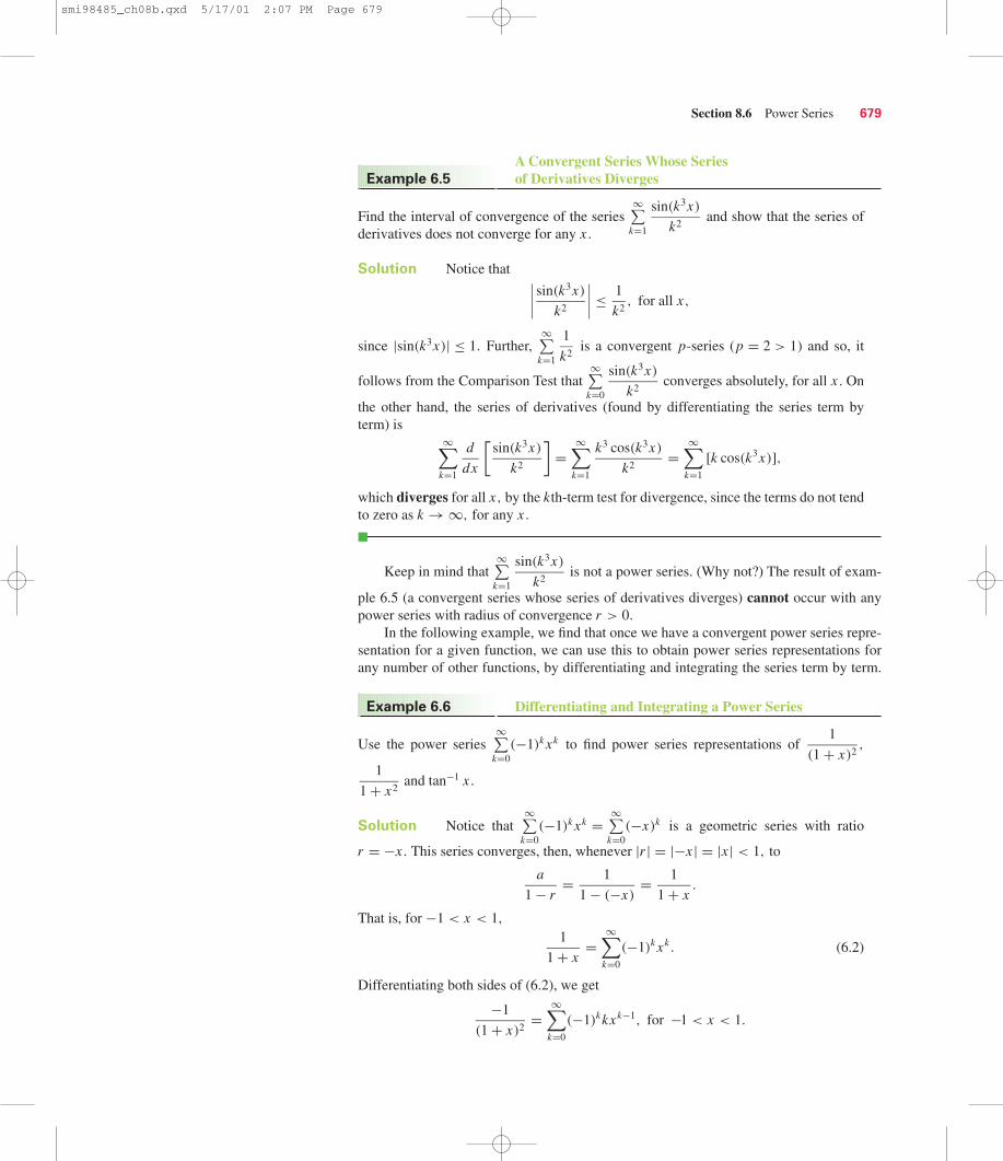
Find the interval of convergence of the series ∞∑

k=1

sin(k3x)

k2and show that the series of

derivatives does not converge for any x .

Solution Notice that ∣∣∣∣ sin(k3x)

k2

∣∣∣∣ ≤ 1

k2, for all x,

since |sin(k3x)| ≤ 1. Further, ∞∑

k=1

1

k2is a convergent p-series (p = 2 > 1) and so, it

follows from the Comparison Test that ∞∑

k=0

sin(k3x)

k2converges absolutely, for all x . On

the other hand, the series of derivatives (found by differentiating the series term byterm) is

∞∑k=1

d

dx

[sin(k3x)

k2

]=

∞∑k=1

k3 cos(k3x)

k2=

∞∑k=1

[k cos(k3x)],

which diverges for all x, by the kth-term test for divergence, since the terms do not tendto zero as k → ∞, for any x .

■

Keep in mind that ∞∑

k=1

sin(k3x)

k2is not a power series. (Why not?) The result of exam-

ple 6.5 (a convergent series whose series of derivatives diverges) cannot occur with anypower series with radius of convergence r > 0.

In the following example, we find that once we have a convergent power series repre-sentation for a given function, we can use this to obtain power series representations forany number of other functions, by differentiating and integrating the series term by term.

Use the power series ∞∑

k=0(−1)k xk to find power series representations of

1

(1 + x)2,

1

1 + x2and tan−1 x .

Solution Notice that ∞∑

k=0(−1)k xk =

∞∑k=0

(−x)k is a geometric series with ratio

r = −x . This series converges, then, whenever |r | = |−x | = |x | < 1, to

a

1 − r= 1

1 − (−x)= 1

1 + x.

That is, for −1 < x < 1,

1

1 + x=

∞∑k=0

(−1)k xk . (6.2)

Differentiating both sides of (6.2), we get

−1

(1 + x)2=

∞∑k=0

(−1)kkxk−1, for −1 < x < 1.

Differentiating and Integrating a Power SeriesExample 6.6

A Convergent Series Whose Series of Derivatives DivergesExample 6.5



Multiplying both sides by −1 gives us a new power series representation:

1

(1 + x)2=

∞∑k=0

(−1)k+1kxk−1,

valid for −1 < x < 1. Notice that we can also obtain a new power series from (6.2) bysubstitution. For instance, if we replace x with x2, we get

1

1 + x2=

∞∑k=0

(−1)k(x2)k =∞∑

k=0

(−1)k x2k, (6.3)

valid for −1 < x2 < 1 (which is equivalent to having x2 < 1 or −1 < x < 1).Integrating both sides of (6.3) gives us∫

1

1 + x2dx =

∞∑k=0

(−1)k∫

x2k dx =∞∑

k=0

(−1)k x2k+1

2k + 1+ c. (6.4)

You should recognize the integral on the left-hand side of (6.4) as tan−1 x . That is,

tan−1 x =∞∑

k=0

(−1)k x2k+1

2k + 1+ c, for −1 < x < 1. (6.5)

Taking x = 0 gives us

tan−1 0 =∞∑

k=0

(−1)k02k+1

2k + 1+ c = c,

so that c = tan−1 0 = 0. Equation (6.5) now gives us a power series representation fortan−1 x, namely:

tan−1 x =∞∑

k=0

(−1)k x2k+1

2k + 1= x − 1

3x3 + 1

5x5 − 1

7x7 + · · · , for −1 < x < 1.

■

Notice that working as in example 6.6, we can produce power series representations ofany number of functions. In section 8.7, we present a systematic method for producingpower series representations for a wide range of functions.


EXERCISES 8.6

1. Power series have the form ∞∑

k=0ak (x − c)k . Explain why

the farther x is from c, the larger the terms of the seriesare and the less likely the series is to converge. Describe howthis general trend relates to the radius of convergence.

2. Applying the Ratio Test to ∞∑

k=0ak (x − c)k requires you

to evaluate limk→∞

∣∣∣∣ak+1

ak(x − c)

∣∣∣∣. For x = c, this limit

equals 0 and the series converges. As x increases or decreases,|x − c| increases. If the series has a finite radius of convergencer > 0, what is the value of the limit when |x − c| = r ? Explainhow the limit changes when |x − c| < r and |x − c| > r and

how this determines the convergence or divergence of theseries.

3. As shown in example 6.2, ∞∑

k=0

10k

k!(x − 1)k converges

for all x . If x = 1001, the value of (x − 1)k = 1000k

gets very large very fast, as k increases. Explain why, for theseries to converge, the value of k! must get large faster than1000k . To illustrate how fast the factorial grows, compute 50!,100! and 200! (if your calculator can).

4. In a power series representation of √

x + 1 about c = 0,explain why the radius of convergence cannot be greater

than 1 (think about the domain of √

x + 1).


In exercises 5–14, find a power series representation of f (x)about c = 0 (refer to example 6.6). Also, determine the radius andinterval of convergence and graph f (x) together with the partial

sums 3∑

k=0ak xk and

6∑k=0

ak xk .

5. f (x) = 2

1 − x6. f (x) = 3

x − 1

7. f (x) = 3

1 + x28. f (x) = 2

1 − x2

9. f (x) = 2x

1 − x310. f (x) = 3x

1 + x2

11. f (x) = 4

1 + 4x12. f (x) = 3

1 − 4x

13. f (x) = 2

4 + x14. f (x) = 3

6 − x

In exercises 15–20, determine the interval of convergence andthe function to which the given power series converges.

15.∞∑

k=0

(x + 2)k 16.∞∑

k=0

(x − 3)k

17.∞∑

k=0

(2x − 1)k 18.∞∑

k=0

(3x + 1)k

19.∞∑

k=0

(−1)k

(x

2

)k

20.∞∑

k=0

3

(x

4

)k

In exercises 21–38, determine the radius and interval ofconvergence.

21.∞∑

k=0

2k

k!(x − 2)k 22.

∞∑k=0

3k

k!xk

23.∞∑

k=0

k

4kxk 24.

∞∑k=0

k

2kxk

25.∞∑

k=1

(−1)k

k3k(x − 1)k 26.

∞∑k=1

(−1)k+1

k4k(x + 2)k

27.∞∑

k=0

k!(x + 1)k 28.∞∑

k=0

k!(x − 2)k

29.∞∑

k=1

1

k(x − 1)k 30.

∞∑k=0

k(x − 2)k

31.∞∑

k=0

k2(x − 3)k 32.∞∑

k=1

1

k2(x + 2)k


33.∞∑

k=0

k!

(2k)!xk 34.

∞∑k=0

(k!)2

(2k)!xk

35.∞∑

k=1

2k

k2(x + 2)k 36.

∞∑k=0

k2

k!(x + 1)k

37.∞∑

k=1

4k

√k

xk 38.∞∑

k=1

(−1)k xk

√k

In exercises 39–46, find a power series representation and radiusof convergence by integrating or differentiating one of the seriesfrom exercises 5–14.

39. f (x) = 3 tan−1 x 40. f (x) = 2 ln(1 − x)

41. f (x) = 2x

(1 − x2)242. f (x) = 3

(x − 1)2

43. f (x) = ln(1 + x2) 44. f (x) = ln(1 + 4x)

45. f (x) = 1

(1 + 4x)246. f (x) = 2

(4 + x)2

In exercises 47–50, find the interval of convergence of the(nonpower) series and the corresponding series of derivatives.

47.∞∑

k=1

cos(k3 x)

k248.

∞∑k=1

cos(x/k)

k

49.∞∑

k=0

ek x 50.∞∑

k=0

e−2k x

51. For any constants a and b > 0, determine the interval and

radius of convergence of ∞∑

k=0

(x − a)k

bk.

52. Prove that if ∞∑

k=0ak xk has radius of convergence r , with 0 <

r < ∞, then ∞∑

k=0ak x2k has radius of convergence

√r .

53. If ∞∑

k=0ak xk has radius of convergence r , with 0 < r < ∞,

determine the radius of convergence of ∞∑

k=0ak (x − c)k for any

constant c.

54. If ∞∑

k=0ak xk has radius of convergence r , with 0 < r < ∞,

determine the radius of convergence of ∞∑

k=0ak

(xb

)kfor any

constant b �= 0.

55. Show that f (x) = x + 1

(1 − x)2=

2x1−x + 1

1 − xhas the power se-

ries representation f (x) = 1 + 3x + 5x2 + 7x3 + 9x4 + · · · .


Find the radius of convergence. Set x = 1

1000and discuss the

interesting decimal representation of 1,001,000

998,001.

56. Use long division to show that1

1 − x= 1 + x + x2 + x3 + · · · .

57. Even great mathematicians can make mistakes. Leonhard Euler

started with the equation x

x − 1+ x

1 − x= 0, rewrote it as

1

1 − 1/x+ x

1 − x= 0, found power series representations for

each function and concluded that · · · + 1

x2+ 1

x+ 1 + x +

x2 + · · · = 0. Substitute x = 1 to show that the conclusion isfalse, then find the mistake in Euler’s derivation.

58. If your CAS or calculator has a command named “Taylor,” useit to verify your answers to exercises 39–46.

59. Note that the radius of convergence in each of exer-cises 5–9 is 1. Given that the functions in exercises 5, 6,

8 and 9 are undefined at x = 1, explain why the radius of


convergence can’t be larger than 1. The restricted radius in ex-ercise 7 can be understood using complex numbers. Show that1 + x2 = 0 for x = ±i, where i = √−1. In general, a com-plex number a + bi is associated with the point (a, b). Find the“distance” between the complex numbers 0 and i by findingthe distance between the associated points (0, 0) and (0, 1).Discuss how this compares to the radius of convergence. Thenuse the ideas in this exercise to quickly conjecture the radiusof convergence of power series with center c = 0 for the func-

tions f (x) = 4

1 + 4x, f (x) = 2

4 + xand f (x) = 2

4 + x2.

60. For each series f (x), compare the intervals of conver-gence of f (x) and

∫f (x) dx , where the antiderivative

is taken term by term. (a) f (x) =∞∑

k=0(−1)k xk ; (b) f (x) =

∞∑k=0

√kxk ; (c) f (x) =

∞∑k=0

1

kxk . As stated in the text, the ra-

dius of convergence remains the same after integration (or dif-ferentiation). Based on the examples in this exercise, does inte-gration make it more or less likely that the series will convergeat the endpoints? Conversely, will differentiation make it moreor less likely that the series will converge at the endpoints?

8.7 TAYLOR SERIES

You may still be wondering about the reason why we have developed series. Each time wehave developed a new concept, we have worked hard to build a case for why we want to dowhat we’re doing. For example, in developing the derivative, we set out to find the slope ofa tangent line and to find instantaneous velocity, only to find that they were essentially thesame thing. When we developed the definite integral, we did so in the course of trying tofind area under the curve. But, we have not yet completely revealed why we’re pursuing se-ries, even though we’ve been developing them for more than five sections now. Well, thepunchline is close at hand. In this section, we develop a compelling reason for consideringseries. They are not merely another mathematical curiosity, but rather, are an essentialmeans for exploring and computing with transcendental functions (e.g., sin x, cos x, ln x,

ex , etc.).

Suppose that the power series ∞∑

k=0bk(x − c)k has radius of convergence r > 0. As

we’ve observed, this means that the series converges absolutely to some function f on theinterval (c − r, c + r). We have

f (x) =∞∑

k=0

bk(x − c)k = b0 + b1(x − c) + b2(x − c)2 + b3(x − c)3 + b4(x − c)4 + · · · ,

for each x ∈ (c − r, c + r). Differentiating term by term, we get that

f ′(x) =∞∑

k=0

bkk(x − c)k−1 = b1 + 2b2(x − c) + 3b3(x − c)2 + 4b4(x − c)3 + · · · ,


again, for each x ∈ (c − r, c + r). Likewise, we get

f ′′(x) =∞∑

k=0

bkk(k − 1)(x − c)k−2 = 2b2 + 3 · 2b3(x − c) + 4 · 3b4(x − c)2 + · · ·

and

f ′′′(x) =∞∑

k=0

bkk(k − 1)(k − 2)(x − c)k−3 = 3 · 2b3 + 4 · 3 · 2b4(x − c) + · · ·

and so on (all valid for c − r < x < c + r ). Notice that if we substitute x = c in each of theabove derivatives, all the terms of the series drop out, except one. We get

f (c) = b0,

f ′(c) = b1,

f ′′(c) = 2b2,

f ′′′(c) = 3! b3

and so on. Observe that in general, we have

f (k)(c) = k! bk . (7.1)

Solving (7.1) for bk, we have

bk = f (k)(c)

k!, for k = 0, 1, 2, . . . .

To summarize, we found that if ∞∑

k=0bk(x − c)k is a convergent power series with radius of

convergence r > 0, then the series converges to some function f that we can write as

f (x) =∞∑

k=0

bk(x − c)k =∞∑

k=0

f (k)(c)

k!(x − c)k, for x ∈ (c − r, c + r).

Now, think about this problem from another angle. Instead of starting with a series,suppose that you start with an infinitely differentiable function, f (i.e., f can be differen-tiated infinitely often). Then, we can construct the series

∞∑k=0

f (k)(c)

k!(x − c)k,

called a Taylor series expansion for f . (See the historical note on Brook Taylor insection 7.2.) There are two important questions we need to answer.

● Does a series constructed in this way converge? If so, what is its radius of convergence?● If the series converges, it converges to a function. What is that function (for instance, is

it f )?

We can answer the first of these questions on a case-by-case basis, usually by applyingthe Ratio Test. The second question will require further insight.

Construct the Taylor series expansion for f (x) = ex , about x = 0 (i.e., take c = 0).

Solution Here, we have the extremely simple case where

f ′(x) = ex , f ′′(x) = ex and so on, f (k)(x) = ex , for k = 0, 1, 2, . . . .

Constructing a Taylor Series ExpansionExample 7.1

Section 8.7 Taylor Series 683

Taylor Series Expansion

of f (x) about x = c


This gives us the Taylor series

∞∑k=0

f (k)(0)

k!(x − 0)k =

∞∑k=0

e0

k!xk =

∞∑k=0

1

k!xk .

From the Ratio Test, we have

limk→∞

∣∣∣∣ak+1

ak

∣∣∣∣ = limk→∞

|x |k+1

(k + 1)!

k!

|x |k = |x | limk→∞

k!

(k + 1)k!

= |x | limk→∞

1

k + 1= |x | (0) = 0 < 1, for all x .

So, the Taylor series∞∑

k=0

1

k!xk converges for all real numbers x .At this point, though, we

do not know the function to which the series converges. (Could it be ex ?)

■

Before we present any further examples of Taylor series, let’s see if we can determinethe function to which a given Taylor series converges. First, notice that the partial sums ofa Taylor series (like any power series) are simply polynomials. We define

Pn(x) =n∑

k=0

f (k)(c)

k!(x − c)k

= f (c) + f ′(c)(x − c) + f ′′(c)2!

(x − c)2 + · · · + f (n)(c)

n!(x − c)n.

Observe that Pn(x) is a polynomial of degree n, as f (k)(c)

k!is a constant for each k. We

refer to Pn as the Taylor polynomial of degree n for f expanded about x = c.

For f (x) = ex , find the Taylor polynomial of degree n expanded about x = 0.

Solution As in example 7.1, we have that f (k)(x) = ex , for all k. So, we have thenth degree Taylor polynomial is

Pn(x) =n∑

k=0

f (k)(0)

k!(x − 0)k =

n∑k=0

e0

k!xk

=n∑

k=0

1

k!xk = 1 + x + x2

2!+ x3

3!+ · · · + xn

n!.

Since we established in example 7.1 that the Taylor series for f (x) = ex about x = 0converges for all x, this says that the sequence of partial sums (i.e., the sequence ofTaylor polynomials) converges for all x . In an effort to determine the function to whichthe Taylor polynomials are converging, we have plotted P1(x), P2(x), P3(x) and P4(x),together with the graph of f (x) = ex in Figures 8.39a–d, respectively.

Notice that as n gets larger, the graphs of Pn(x) appear (at least on the interval dis-played) to be approaching the graph of f (x) = ex . Since we know that the Taylor seriesconverges and the graphical evidence suggests that the partial sums of the series areapproaching f (x) = ex , it is reasonable to conjecture that the series converges to ex .

Constructing and Graphing Taylor PolynomialsExample 7.2


x2 4�2

�2

2

4

6

8y � ex

y � P1(x)

y

Figure 8.39a

y = ex and y = P1(x).

The special case of a Taylor seriesexpansion about x = 0 is oftencalled a Maclaurin series. (See thehistorical note about Colin Maclau-rin in section 8.3.) That is, the series∞∑

k=0

f (k)(0)

k!xk is the Maclaurin series

expansion for f .

Remark 5.3


This is, in fact, exactly what is happening, as we can prove using the following twotheorems.

■

The error term Rn(x) in (7.2) is often called the remainder term. Note that this termlooks very much like the first neglected term of the Taylor series, except that f (n+1) is eval-uated at some (unknown) number z between x and c, instead of at c. This remainder termserves two purposes: it enables us to obtain an estimate of the error in using a Taylor poly-nomial to approximate a given function and as we’ll see in the next theorem, it gives us themeans to prove that a Taylor series for a given function f converges to f .

The proof of Taylor’s Theorem is somewhat technical and so we leave it for the end ofthe section.

Note: If we could show that

limn→∞ Rn(x) = 0, for all x in (c − r, c + r),

then we would have that

0 = limn→∞ Rn(x) = lim

n→∞[ f (x) − Pn(x)] = f (x) − limn→∞ Pn(x)

or

limn→∞ Pn(x) = f (x), for all x ∈ (c − r, c + r).

Theorem 7.1 (Taylor’s Theorem)

Suppose that f has (n + 1) derivatives on the interval (c − r, c + r), for some r > 0.

Then, for x ∈ (c − r, c + r), f (x) ≈ Pn(x) and the error in using Pn(x) to approximatef (x) is

Rn(x) = f (x) − Pn(x) = f (n+1)(z)

(n + 1)!(x − c)n+1, (7.2)

for some number z between x and c.


x2 4�2

�2

2

4

6

8 y � ex

y � P2(x)

y

Figure 8.39b


x2 4�2

�2

2

4

6

8y � ex

y � P3(x)

y

Figure 8.39c


x2 4�2

�2

2

4

6

8 y � ex

y � P4(x)

y

Figure 8.39d



That is, the sequence of partial sums of the Taylor series (i.e., the sequence of Taylor poly-nomials) converges to f (x) for each x ∈ (c − r, c + r). We summarize this in Theorem 7.2.

We now return to the Taylor series expansion of f (x) = ex about x = 0, constructedin example 7.1 and investigated further in example 7.2 and prove that it converges to ex , aswe had suspected.

Show that the Taylor series for f (x) = ex expanded about x = 0 converges to ex .

Solution We already found the indicated Taylor series, ∞∑

k=0

1

k!xk in example 7.1.

Here, we have f (k)(x) = ex , for all k = 0, 1, 2, . . . . This gives us the remainder term

Rn(x) = f (n+1)(z)

(n + 1)!(x − 0)n+1 = ez

(n + 1)!xn+1, (7.3)

where z is somewhere between x and 0 (and depends also on the value of n). We firstfind a bound on the size of ez. Notice that if x > 0, then 0 < z < x and so,

ez < ex .

If x ≤ 0, then x ≤ z ≤ 0, so that

ez ≤ e0 = 1.

We define M to be the larger of these two bounds on ez. That is, we let

M = max{ex , 1}.Then, for any x and any n, we have

ez ≤ M.

Together with (7.3), this gives us the error estimate

|Rn(x)| = ez

(n + 1)!|x |n+1 ≤ M

|x |n+1

(n + 1)!. (7.4)

To prove that the Taylor series converges to ex , we want to use (7.4) to show thatlim

n→∞ Rn(x) = 0, for all x . However, for any given x, how can we compute

limn→∞

|x |n+1

(n + 1)!? While we cannot do so directly, we can use the following indirect

approach. We consider the series∞∑

n=0

|x |n+1

(n + 1)!as follows. Applying the Ratio Test,

Proving That a Taylor Series Convergesto the Desired FunctionExample 7.3

Theorem 7.2

Suppose that f has derivatives of all orders in the interval (c − r, c + r), for somer > 0 and lim

n→∞ Rn(x) = 0, for all x in (c − r, c + r). Then, the Taylor series for f

expanded about x = c converges to f (x), that is,

f (x) =∞∑

k=0

f (k)(c)

k!(x − c)k,

for all x in (c − r, c + r).


Observe that for n = 0, Taylor’sTheorem simplifies to a very familiarresult. We have

R0(x) = f (x) − P0(x) =f ′(z)

(0 + 1)!(x − c)0+1.

Since P0(x) = f (c), we have simply

f (x) − f (c) = f ′(z)(x − c).

Dividing by (x − c), gives us

f (x) − f (c)

x − c= f ′(z),

which is the conclusion of the MeanValue Theorem. In this way, observethat Taylor’s Theorem is a general-ization of the Mean Value Theorem.

Remark 7.2


we have

limn→∞

∣∣∣∣an+1

an

∣∣∣∣ = limn→∞

|x |n+2

(n + 2)!

(n + 1)!

|x |n+1= |x | lim

n→∞1

n + 2= 0,

for all x . This then says that the series ∞∑

n=0

|x |n+1

(n + 1)!converges absolutely for all x . By

the kth-term test for divergence, since this last series converges, its general term musttend to 0 as n → ∞. That is,

limn→∞

|x |n+1

(n + 1)!= 0

and so, from (7.4), limn→∞ Rn(x) = 0, for all x . From Theorem 7.2, we now have that the

Taylor series converges to ex for all x. That is,

(7.5)

■

The trick, if there is one, in finding a Taylor series expansion is in accurately calcu-lating enough derivatives for you to recognize the general form of the nth derivative. So,take your time and BE CAREFUL! Once this is done, you need only show thatRn(x) → 0, as n → ∞, for all x to ensure that the series converges to the function youare expanding.

One of the reasons for calculating Taylor series is that we can use their partial sums tocompute approximate values of a function.

Use the Taylor series for ex in (7.5) to obtain an approximation to the number e.

Solution We have

e = e1 =∞∑

k=0

1

k!1k =

∞∑k=0

1

k!.

We list some partial sums of this series in the accompanying table. From this we get thevery accurate approximation

e ≈ 2.718281828.

■

Find the Taylor series for f (x) = sin x, expanded about x = π2 and prove that the series

converges to sin x for all x .

Solution In this case, the Taylor series is

∞∑k=0

f (k)(

π2

)k!

(x − π

2

)k

.

A Taylor Series Expansion of sin xExample 7.5

Using a Taylor Series to Obtain an Approximation of eExample 7.4

ex =∞∑

k=0

1

k!xk = 1 + x + x2

2!+ x3

3!+ x4

4!+ · · · .


MM∑

k=0

1k!

5 2.716666667

10 2.718281801

15 2.718281828

20 2.718281828


First, we compute some derivatives and their value at x = π2 . We have

f (x) = sin x f(

π2

) = 1,

f ′(x) = cos x f ′(π2

) = 0,

f ′′(x) = −sin x f ′′(π2

) = −1,

f ′′′(x) = −cos x f ′′′(π2

) = 0,

f (4)(x) = sin x f (4)(

π2

) = 1

and so on. Recognizing that every other term is zero and every other term is ±1, we seethat the Taylor series is

∞∑k=0

f (k)(

π2

)k!

(x − π

2

)k

= 1 − 1

2

(x − π

2

)2

+ 1

4!

(x − π

2

)4

− 1

6!

(x − π

2

)6

+ · · ·

=∞∑

k=0

(−1)k

(2k)!

(x − π

2

)2k

.

In order to test the series for convergence, we consider the remainder term

|Rn(x)| =∣∣∣∣∣ f (n+1)(z)

(n + 1)!

(x − π

2

)n+1∣∣∣∣∣ , (7.6)

for some z between x and π2 . From our derivative calculations, note that

f (n+1)(z) ={±cos z, if n is even

±sin z, if n is odd.

From this, it follows that ∣∣ f (n+1)(z)∣∣ ≤ 1,

for every n. (Notice that this is true whether n is even or odd.) From (7.6), we now have

|Rn(x)| =∣∣∣∣ f (n+1)(z)

(n + 1)!

∣∣∣∣∣∣∣∣x − π

2

∣∣∣∣n+1

≤ 1

(n + 1)!

∣∣∣∣x − π

2

∣∣∣∣n+1

→ 0,

as n → ∞, for every x, as in example 7.3. This says that

for all x . In Figures 8.40a–d, we show graphs of f (x) = sin x together with the Taylorpolynomials P2(x), P4(x), P6(x) and P8(x) (the first few partial sums of the series).Notice that the higher the degree of the Taylor polynomial is, the larger the interval isover which the polynomial provides a close approximation to f (x) = sin x .

sin x =∞∑

k=0

(−1)k

(2k)!

(x − π

2

)2k

= 1 − 1

2

(x − π

2

)2

+ 1

4!

(x − π

2

)4

− · · · ,



■

In the following example, we illustrate how to use Taylor’s Theorem to estimate theerror in using a Taylor polynomial to approximate the value of a function.

Use a Taylor polynomial to approximate the value of ln(1.1) and estimate the error inthis approximation.

Solution First, note that since ln 1 is known exactly and 1 is close to 1.1 (whywould this matter?), we expand f (x) = ln x in a Taylor series about x = 1. We computean adequate number of derivatives so that the pattern becomes clear. We have

f (x) = ln x f (1) = 0

f ′(x) = x−1 f ′(1) = 1

f ′′(x) = −x−2 f ′′(1) = −1

f ′′′(x) = 2x−3 f ′′′(1) = 2

f (4)(x) = −3 · 2x−4 f (4)(1) = −3!

f (5)(x) = 4! x−5 f (5)(1) = 4!...

...

f (k)(x) = (−1)k+1(k − 1)! x−k f (k)(1) = (−1)k+1(k − 1)!

Estimating the Error in a TaylorPolynomial ApproximationExample 7.6


y

x2 4 6�2

�1

1

y � sin xy � P2(x)

Figure 8.40a

y = sin x and y = P2(x).

y

x2 4 6�2

�1

1

y � sin x

y � P4(x)

Figure 8.40b


y

x2 4 6�2

�1

1

y � sin x

y � P6(x)

Figure 8.40c


y

x2 4 6�2

�1

1

y � sin x

y � P8(x)

Figure 8.40d



We get the Taylor series

∞∑k=0

f (k)(1)

k!(x − 1)k

= (x − 1) − 1

2(x − 1)2 + 2

3!(x − 1)3 + · · · + (−1)k+1 (k − 1)!

k!(x − 1)k + · · ·

=∞∑

k=1

(−1)k+1

k(x − 1)k .

We could use the remainder term to show that the series converges to f (x) = ln x, for0 < x < 2, but this is not the original question here. (This is left as an exercise.) As anillustration, we construct the Taylor polynomial, P4(x),

P4(x) =4∑

k=0

(−1)k+1

k(x − 1)k

= (x − 1) − 1

2(x − 1)2 + 1

3(x − 1)3 − 1

4(x − 1)4.

We show a graph of y = ln x and y = P4(x) in Figure 8.41. Taking x = 1.1 gives us theapproximation

ln(1.1) ≈ P4(1.1) = 0.1 − 1

2(0.1)2 + 1

3(0.1)3 − 1

4(0.1)4 ≈ 0.095308333.

We can use the remainder term to estimate the error in this approximation. We have

|Error| = |ln(1.1) − P4(1.1)| = |R4(1.1)|

=∣∣∣∣ f (4+1)(z)

(4 + 1)!(1.1 − 1)4+1

∣∣∣∣ = 4! |z|−5

5!(0.1)5,

where z is between 1 and 1.1. This gives us the following bound on the error:

|Error| = (0.1)5

5z5<

(0.1)5

5(15)= 0.000002,

since 1 < z < 1.1 implies that 1

z<

1

1= 1. Another way to think of this is that our

approximation of ln(1.1) ≈ 0.095308333 is off by no more than ±0.000002.

■

A more significant problem related to example 7.6 is to determine how many terms ofthe Taylor series are needed in order to guarantee a given accuracy. We use the remainderterm to accomplish this in the following example.

Find the number of terms in the Taylor series for f (x) = ln x expanded about x = 1 thatwill guarantee an accuracy of at least 1 × 10−10 in the approximation of ln(1.1) andln(1.5).

Finding the Number of Terms Neededfor a Given AccuracyExample 7.7

from above


2 31

2

�2

�4

y � ln x

y � P4(x)

y

x

Figure 8.41

y = ln x and y = P4(x).


Solution From our calculations in example 7.6 and (7.2), we have that for somenumber z between 1 and 1.1,

|Rn(1.1)| =∣∣∣∣ f (n+1)(z)

(n + 1)!(1.1 − 1)n+1

∣∣∣∣= n! |z|−n−1

(n + 1)!(0.1)n+1 = (0.1)n+1

(n + 1)zn+1<

(0.1)n+1

n + 1,


z<

1

1= 1. Further, since we want the error to be less

than 1 × 10−10, we require that

|Rn(1.1)| <(0.1)n+1

n + 1< 1 × 10−10.

You can solve this inequality for n by trial and error to find that n = 9 will guarantee therequired accuracy. Notice that larger values of n will also guarantee this accuracy, since(0.1)n+1

n + 1is a decreasing function of n. We then have the approximation

ln(1.1) ≈ P9(1.1) =9∑

k=0

(−1)k+1

k(1.1 − 1)k

= (0.1) − 1

2(0.1)2 + 1

3(0.1)3 − 1

4(0.1)4 + 1

5(0.1)5

−1

6(0.1)6 + 1

7(0.1)7 − 1

8(0.1)8 + 1

9(0.1)9

≈ 0.095310179813,

which from our error estimate we know is correct to within 1 × 10−10. We show a graphof y = ln x and y = P9(x) in Figure 8.42. In comparing Figure 8.42 with Figure 8.41,observe that while P9(x) provides an improved approximation to P4(x) over the inter-val of convergence (0, 2), it does not provide a better approximation outside of thisinterval.

Similarly, notice that for some number z between 1 and 1.5,

|Rn(1.5)| =∣∣∣∣ f (n+1)(z)

(n + 1)!(1.5 − 1)n+1

∣∣∣∣ = n! |z|−n−1

(n + 1)!(0.5)n+1

= (0.5)n+1

(n + 1)zn+1<

(0.5)n+1

n + 1,


z<

1

1= 1. So, here we require that

|Rn(1.5)| <(0.5)n+1

n + 1< 1 × 10−10.

Solving this by trial and error shows that n = 28 will guarantee the required accuracy.Observe that this says that many more terms are needed to approximate f (1.5) than forf (1.1), to obtain the same accuracy. This further illustrates the general principle that thefarther away x is from the point about which we expand, the slower the convergence ofthe Taylor series will be.

■


y

x1 2 3

�2

�4

2

y � ln x

y � P9(x)

Figure 8.42

y = ln x and y = P9(x).


For your convenience, we have compiled a list of common Taylor series in the fol-lowing table.


Interval ofTaylor Series Convergence Where to find

Notice that once you have found a Taylor series expansion for a given function, youcan find any number of other Taylor series simply by making a substitution.

Find Taylor series in powers of x for e2x , ex2and e−x .

Solution Rather than compute the Taylor series for these functions from scratch,recall that we had established in example 7.3 that

et =∞∑

k=0

1

k!t k = 1 + t + 1

2!t2 + 1

3!t3 + 1

4!t4 + · · · , (7.7)

for all t ∈ (−∞,∞). We use the variable t here instead of x, so that we can more easilymake substitutions. Taking t = 2x in (7.7), we get the new Taylor series:

e2x =∞∑

k=0

1

k!(2x)k =

∞∑k=0

2k

k!xk = 1 + 2x + 22

2!x2 + 23

3!x3 + · · · .

Similarly, letting t = x2 in (7.7), we get the Taylor series

ex2 =∞∑

k=0

1

k!(x2)k =

∞∑k=0

1

k!x2k = 1 + x2 + 1

2!x4 + 1

3!x6 + · · · .

Finally, taking t = −2x in (7.7), we get

e−2x =∞∑

k=0

1

k!(−2x)k =

∞∑k=0

(−1)k

k!2k xk = 1 − 2x + 22

2!x2 − 23

3!x3 + · · · .

Notice that all of these last three series converge for all x ∈ (−∞,∞). (Why is that?)

■

Finding New Taylor Series from Old OnesExample 7.8

ex =∞∑

k=0

1

k!xk = 1 + x + 1

2x2 + 1

3!x3 + 1

4!x4 + · · · (−∞,∞) examples 7.1 and 7.3

sin x =∞∑

k=0

(−1)k

(2k + 1)!x2k+1 = x − 1

3!x3 + 1

5!x5 − 1

7!x7 + · · · (−∞,∞) exercise 9

cos x =∞∑

k=0

(−1)k

(2k)!x2k = 1 − 1

2x2 + 1

4!x4 − 1

6!x6 + · · · (−∞,∞) exercise 7

sin x =∞∑

k=0

(−1)k

(2k)!

(x − π

2

)2k

= 1 − 1

2

(x − π

2

)2

+ 1

4!

(x − π

2

)4

− · · · (−∞,∞) example 7.5

ln x =∞∑

k=1

(−1)k+1

k(x − 1)k = (x − 1) − 1

2(x − 1)2 + 1

3(x − 1)3 − · · · (0, 2] examples 7.6, 7.7

tan−1 x =∞∑

k=0

(−1)k

2k + 1x2k+1 = x − 1

3x3 + 1

5x5 − 1

7x7 + · · · (−1, 1) example 6.6


Proof of Taylor’s TheoremRecall that we had observed that the Mean Value Theorem was a special case of Taylor’s The-orem. As it turns out, the proof of Taylor’s Theorem parallels that of the Mean Value Theorem.Both make use of Rolle’s Theorem: If g is continuous on the interval [a, b], differentiable on(a, b) and g(a) = g(b), then there is a number c ∈ (a, b) for which g′(c) = 0. As with theproof of the Mean Value Theorem, for a fixed x ∈ (c − r, c + r), we define the function

g(t) = f (x) − f (t) − f ′(t)(x − t) − 1

2!f ′′(t)(x − t)2 − 1

3!f ′′′(t)(x − t)3

− · · · − 1

n!f (n)(t)(x − t)n − Rn(x)

(x − t)n+1

(x − c)n+1,

where Rn(x) is the remainder term, Rn(x) = f (x) − Pn(x). If we take t = x, notice that

g(x) = f (x) − f (x) − 0 − 0 − · · · − 0 = 0

and if we take t = c, we get

g(c) = f (x) − f (c) − f ′(c)(x − c) − 1

2!f ′′(c)(x − c)2 − 1

3!f ′′′(c)(x − c)3

− · · · − 1

n!f (n)(c)(x − c)n − Rn(x)

(x − c)n+1

(x − c)n+1

= f (x) − Pn(x) − Rn(x) = Rn(x) − Rn(x) = 0.

By Rolle’s Theorem, there must be some number z between x and c for which g′(z) = 0.

Differentiating our expression for g(t) (with respect to t!), we get (beware of all theproduct rules!)

g′(t) = 0 − f ′(t) − f ′(t)(−1) − f ′′(t)(x − t) − 1

2f ′′(t)(2)(x − t)(−1)

− 1

2f ′′′(t)(x − t)2 − · · · − 1

n!f (n)(t)(n)(x − t)n−1(−1)

− 1

n!f (n+1)(t)(x − t)n − Rn(x)

(n + 1)(x − t)n(−1)

(x − c)n+1

= − 1

n!f (n+1)(t)(x − t)n + Rn(x)

(n + 1)(x − t)n

(x − c)n+1,

after most of the terms cancel. So, taking t = z, we have that

0 = g′(z) = − 1

n!f (n+1)(z)(x − z)n + Rn(x)

(n + 1)(x − z)n

(x − c)n+1.

Solving this for the remainder term, Rn(x), we get

Rn(x)(n + 1)(x − z)n

(x − c)n+1= 1

n!f (n+1)(z)(x − z)n

and finally,

Rn(x) = 1

n!f (n+1)(z)(x − z)n (x − c)n+1

(n + 1)(x − z)n

= f (n+1)(z)

(n + 1) n!(x − c)n+1

= f (n+1)(z)

(n + 1)!(x − c)n+1,

as we had claimed.



EXERCISES 8.7


1. Describe how the Taylor polynomial with n = 1 com-pares to the linear approximation (see section 3.1). Give

an analogous interpretation of the Taylor polynomial withn = 2. That is, how do various graphical properties (position,slope, concavity) of the Taylor polynomial compare with thoseof the function f (x) at x = c?

2. Briefly discuss how a computer might use Taylorpolynomials to compute sin(1.2). In particular, how

would the computer know how many terms to compute? Howwould the number of terms necessary to compute sin(1.2)

compare to the number needed to compute sin(100)? Describea trick that would make it much easier for the computer tocompute sin(100). (Hint: The sine function is periodic.)

3. Taylor polynomials are built up from a knowledge off (c), f ′(c), f ′′(c) and so on. Explain in graphical terms

why information at one point (e.g., position, slope, concavity,etc.) can be used to construct the graph of the function on theentire interval of convergence.

4. If f (c) is the position of an object at time t = c, thenf ′(c) is the object’s velocity and f ′′(c) is the object’s

acceleration at time c. Explain in physical terms howknowledge of these values at one time (plus f ′′′(c), etc.) can beused to predict the position of the object on the interval ofconvergence.

5. Our table of common Taylor series lists two different se-ries for sin x . Explain how the same function could have

two different Taylor series representations. For a given problem(e.g., approximate sin 2), explain how you would choose whichTaylor series to use.

6. Explain why the Taylor series with center c = 0 off (x) = x2 − 1 is simply x2 − 1.

In exercises 7–14, find the Maclaurin series (i.e., Taylor seriesabout c = 0) and its interval of convergence.

7. f (x) = cos x 8. f (x) = e2x

9. f (x) = sin x 10. f (x) = cos 2x

11. f (x) = ln(1 + x) 12. f (x) = e−x

13. f (x) = 1/(1 + x)2 14. f (x) = 1/(1 − x)

In exercises 15–20, find the Taylor series about the indicated cen-ter and determine the interval of convergence.

15. f (x) = ex−1 , c = 1 16. f (x) = cos x , c = −π/2

17. f (x) = ln x , c = e 18. f (x) = ex , c = 2

19. f (x) = 1/x , c = 1 20. f (x) = 1/x , c = −1

In exercises 21–28, graph f (x) and the Taylor polynomials forthe indicated center c and degree n.

21. f (x) = cos x , c = 0, n = 5; n = 9

22. f (x) = ln x , c = 1, n = 4; n = 8

23. f (x) = √x , c = 1, n = 3; n = 6

24. f (x) = 1

1 + x, c = 0, n = 4; n = 8

25. f (x) = ex , c = 2, n = 3; n = 6

26. f (x) = cos x , c = π/2, n = 4; n = 8

27. f (x) = 1√x

, c = 4, n = 2; n = 4

28. f (x) = √1 + x2 , c = 0, n = 2; n = 4

In exercises 29–32, prove that the Taylor series converges to f (x)by showing that Rn(x)→ 0 as n→∞.

29. sin x =∞∑

k=0

(−1)k x2k+1

(2k + 1)!

30. cos x =∞∑

k=0

(−1)k x2k

(2k)!

31. ln x =∞∑

k=1

(−1)k+1 (x − 1)k

k, 1 ≤ x ≤ 2

32. e−x =∞∑

k=0

(−1)k xk

k!

In exercises 33–38, (a) use a Taylor polynomial of degree 4 toapproximate the given number, (b) estimate the error in theapproximation, (c) estimate the number of terms needed in aTaylor polynomial to guarantee an accuracy of 10−10 .

33. ln(1.05) 34. ln(0.9) 35.√

1.1

36.√

1.2 37. e0.1 38. e−0.1

In exercises 39–44, use a Taylor series to verify the givenformula.

39.∞∑

k=0

2k

k!= e2 40.

∞∑k=0

(−1)k

k!= e−1


41.∞∑

k=0

(−1)kπ2k+1

(2k + 1)!= 0 42.

∞∑k=0

(−1)k (π/2)2k+1

(2k + 1)!= 1

43.∞∑

k=0

(−1)k

2k + 1= π

444.

∞∑k=1

(−1)k+1

k= ln 2

In exercises 45–52, use a known Taylor series to find the Taylorseries about c = 0 for the given function and find its radius ofconvergence.

45. f (x) = e−2x 46. f (x) = e3x

47. f (x) = xe−x 248. f (x) = ex − 1

x

49. f (x) = sin x2 50. f (x) = x sin 2x

51. f (x) = cos 3x 52. f (x) = cos x3

53. You may have wondered why it is necessary to show thatlim

n→∞Rn (x) = 0 to conclude that a Taylor series converges

to f (x). Consider f (x) ={

e−1/x 2, if x �= 0

0, if x = 0. Show that

f ′(0) = f ′′(0) = 0. (Hint: Use the fact that limn→0

e−1/n2

nn= 0

for any positive integer n.) It turns out that f (n)(0) = 0 for alln. Thus, the Taylor series of f (x) about c = 0 equals 0, a con-vergent “series’’ which does not converge to f (x).

54. In many applications the error function erf(x) =2√π

∫ x

0e−u2

du is important. Compute and graph the fourth-

order Taylor polynomial for erf(x) about c = 0.

55. Suppose that a plane is at location f (0) = 10 miles with veloc-ity f ′(0) = 10 miles/min, acceleration f ′′(0) = 2 miles/min2

and f ′′′(0) = −1 miles/min3. Predict the location of the planeat time t = 2 min.

56. Suppose that an astronaut is at (0, 0) and the moon is repre-sented by a circle of radius 1 centered at (10, 5). The astro-naut’s capsule follows a path y = f (x) with current position

Section 8.8 Applications of Taylor Series 695

f (0) = 0, slope f ′(0) = 1/5, concavity f ′′(0) = −1/10,f ′′′(0) = 1/25, f (4)(0) = 1/25 and f (5)(0) = −1/50. Graph aTaylor polynomial approximation of f (x). Based on your cur-rent information, do you advise the astronaut to change paths?How confident are you in the accuracy of your approximation?

57. Find the Taylor series for ex about a general center c.

58. Find the Taylor series for √

x about a general center c = a2.

Exercises 59–62 involve the binomial expansion.

59. Show that the Maclaurin series for (1 + x)r is

1 +∞∑

k=1

r(r − 1) · · · (r − k + 1)

k!xk for any constant r .

60. Simplify the series in exercise 59 for r = 2; r = 3; r is a posi-tive integer.

61. Use the result of exercise 59 to write out the Maclaurin seriesfor f (x) = √

1 + x .

62. Use the result of exercise 59 to write out the Maclaurin seriesfor f (x) = (1 + x)3/2.

63. Find the Maclaurin series of f (x) = cosh x and f (x) = sinh x .

Compare to the Maclaurin series of cos x and sin x .

64. Use the Maclaurin series for tan x and the result of exercise 63to conjecture the Maclaurin series for tanh x .

65. Almost all of our series results apply to series ofcomplex numbers. Defining i = √−1, show that

i2 = −1, i3 = −i, i4 = 1, and so on. Replacing x with i x inthe Maclaurin series for ex , separate terms containing i fromthose that don’t contain i (after the simplifications indicatedabove) and derive Euler’s formula ei x = cos x + i sin x .

66. Using the technique of exercise 65, show that cos(i x) =cosh x and sin(i x) = i sinh x . That is, the trig functions

and their hyperbolic counterparts are closely related as func-tions of complex variables.

8.8 APPLICATIONS OF TAYLOR SERIES

In section 8.7, we developed the concept of a Taylor series expansion and gave many illus-trations of how to compute Taylor series expansions. We also gave a few hints as to howthese expansions might be used. In this section, we expand on our earlier presentation, bygiving a few examples of how Taylor series are used in applications. You probably recog-nize that the work in the preceding section was challenging. The good news is that yourhard work has significant payoffs, as we illustrate with the following problems. It’s worth


noting that many of the early practitioners of the calculus (including Newton and Leibniz)worked actively with series.

In this section, we will use series to approximate the values of transcendental func-tions, evaluate limits and integrals and define important new functions. As you continueyour studies in mathematics and related fields, you are likely to see far more applicationsof Taylor series than we can include here.

In the introduction to this chapter, we asked you to consider how calculators and com-puters might calculate values of transcendental functions, like sin(1.234567). We can nowdo so using Taylor series.

Use a Taylor series to compute sin(1.234567) accurate to within 10−11.

Solution It’s not hard to find the Taylor series expansion for f (x) = sin x aboutx = 0. (We left this as an exercise in section 8.7.) We have

sin x =∞∑

k=0

(−1)k

(2k + 1)!x2k+1 = x − 1

3!x3 + 1

5!x5 − 1

7!x7 + · · · ,

where the interval of convergence is (−∞,∞). Notice that if we take x = 1.234567,the series representation of sin 1.234567 is

sin 1.234567 =∞∑

k=0

(−1)k

(2k + 1)!(1.234567)2k+1,

which is an alternating series. We can use a partial sum of this series to approximate thedesired value, but just how accurate will a given partial sum be? Recall that for alternat-ing series, the error in a partial sum is bounded by the absolute value of the firstneglected term. (Note that you could also use the remainder term from Taylor’s Theoremto bound the error.) To ensure that the error is less than 10−11, we must find an integer k

such that 1.2345672k+1

(2k + 1)!< 10−11 . By trial and error, we find that

1.23456717

17!≈ 1.010836 × 10−13 < 10−11,

so that k = 8 will do. Observe that this says that the first neglected term corresponds tok = 8 and so, we compute the partial sum

sin 1.234567 ≈7∑

k=0

(−1)k

(2k + 1)!(1.234567)2k+1

= 1.234567 − 1.2345673

3!+ 1.2345675

5!− 1.2345677

7!+ · · · − 1.23456715

15!

≈ 0.94400543137.

Check your calculator or computer to verify that this matches your calculator’s estimate.

■

If you look carefully at example 8.1, you might discover that we were a bit hasty.Certainly, we answered the question and produced an approximation with the desiredaccuracy, but was this the easiest way in which to do this? The answer is no, as we simplygrabbed the most handy Taylor series expansion of f (x) = sin x . You should try to resist theimpulse to automatically use the Taylor series expansion about x = 0 (i.e., the Maclaurinseries), rather than making a more efficient choice. We illustrate this in the following example.

Using Taylor Polynomials to Approximate a Sine ValueExample 8.1



Repeat example 8.1, but this time, make a more appropriate choice of the Taylor series.

Solution Recall from our discussion in section 8.7 that Taylor series convergemuch faster close to the point about which you expand, than they do far away. So, if weneed to compute sin 1.234567, is there a handy Taylor series expansion of f (x) = sin xabout some point closer to x = 1.234567? Keeping in mind that we only know the valueof sin x exactly at a few points, you should quickly recognize that a series expandedabout x = π

2 ≈ 1.57 is a better choice than one expanded about x = 0. (Anotherreasonable choice is the Taylor series expansion about x = π

3 .) In example 7.5, recallthat we had found that

sin x =∞∑

k=0

(−1)k

(2k)!

(x − π

2

)2k

= 1 − 1

2

(x − π

2

)2

+ 1

4!

(x − π

2

)4

− · · · ,

where the interval of convergence is (−∞,∞). Taking x = 1.234567, gives us

sin 1.234567 =∞∑

k=0

(−1)k

(2k)!

(1.234567 − π

2

)2k

= 1 − 1

2

(1.234567 − π

2

)2

+ 1

4!

(1.234567 − π

2

)4

− · · · ,

which, is again an alternating series. Using the remainder term from Taylor’s Theoremto bound the error, we have that

|Rn(1.234567)| =∣∣∣∣ f (2n+2)(z)

(2n + 2)!

∣∣∣∣∣∣∣∣1.234567 − π

2

∣∣∣∣2n+2

≤∣∣1.234567 − π

2

∣∣2n+2

(2n + 2)!.

(Note that we might also have chosen to use Theorem 4.2.) By trial and error, you canfind that ∣∣1.234567 − π

2

∣∣2n+2

(2n + 2)!< 10−11

for n = 4, so that an approximation with the required degree of accuracy is

sin 1.234567 ≈4∑

k=0

(−1)k

(2k)!

(1.234567 − π

2

)2k

= 1 − 1

2

(1.234567 − π

2

)2

+ 1

4!

(1.234567 − π

2

)4

− 1

6!

(1.234567 − π

2

)6

+ 1

8!

(1.234567 − π

2

)8

≈ 0.94400543137.

Compare this result to example 8.1, where we needed to compute many more terms ofthe Taylor series to obtain the same degree of accuracy.

■

We can also use Taylor series to quickly conjecture the value of difficult limits. Be care-ful, though: the theory of when these conjectures are guaranteed to be correct is beyond thelevel of this text. However, we can certainly obtain helpful hints about certain limits.

Choosing a More Appropriate Taylor Series ExpansionExample 8.2



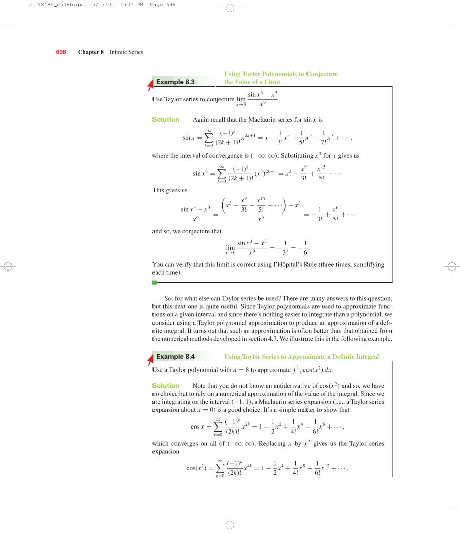
Use Taylor series to conjecture limx→0

sin x3 − x3

x9.

Solution Again recall that the Maclaurin series for sin x is

sin x =∞∑

k=0

(−1)k

(2k + 1)!x2k+1 = x − 1

3!x3 + 1

5!x5 − 1

7!x7 + · · · ,

where the interval of convergence is (−∞,∞). Substituting x3 for x gives us

sin x3 =∞∑

k=0

(−1)k

(2k + 1)!(x3)2k+1 = x3 − x9

3!+ x15

5!− · · ·

This gives us

sin x3 − x3

x9=

(x3 − x9

3!+ x15

5!− · · ·

)− x3

x9= − 1

3!+ x6

5!+ · · ·

and so, we conjecture that

limx→0

sin x3 − x3

x9= − 1

3!= −1

6.

You can verify that this limit is correct using l’Hôpital’s Rule (three times, simplifyingeach time).

■

So, for what else can Taylor series be used? There are many answers to this question,but this next one is quite useful. Since Taylor polynomials are used to approximate func-tions on a given interval and since there’s nothing easier to integrate than a polynomial, weconsider using a Taylor polynomial approximation to produce an approximation of a defi-nite integral. It turns out that such an approximation is often better than that obtained fromthe numerical methods developed in section 4.7. We illustrate this in the following example.

Use a Taylor polynomial with n = 8 to approximate ∫ 1−1 cos(x2) dx .

Solution Note that you do not know an antiderivative of cos(x2) and so, we haveno choice but to rely on a numerical approximation of the value of the integral. Since weare integrating on the interval (−1, 1), a Maclaurin series expansion (i.e., a Taylor seriesexpansion about x = 0) is a good choice. It’s a simple matter to show that

cos x =∞∑

k=0

(−1)k

(2k)!x2k = 1 − 1

2x2 + 1

4!x4 − 1

6!x6 + · · · ,

which converges on all of (−∞,∞). Replacing x by x2 gives us the Taylor seriesexpansion

cos(x2) =∞∑

k=0

(−1)k

(2k)!x4k = 1 − 1

2x4 + 1

4!x8 − 1

6!x12 + · · · ,

Using Taylor Series to Approximate a Definite IntegralExample 8.4

Using Taylor Polynomials to Conjecture the Value of a LimitExample 8.3



so that

cos(x2) ≈ 1 − 1

2x4 + 1

4!x8.

This leads us to the approximation∫ 1

−1cos(x2) dx ≈

∫ 1

−1

(1 − 1

2x4 + 1

4!x8

)dx

=(

x − x5

10+ x9

216

) ∣∣∣∣x=1

x=−1

= 977

540≈ 1.809259.

Our CAS gives us ∫ 1−1 cos(x2) dx ≈ 1.809048, so our approximation appears to be very

accurate.

■

You might reasonably argue that we don’t need Taylor series to obtain approximationslike those in example 8.4, as you could always use other, simpler numerical methods likeSimpson’s Rule to do the job. That’s often true, but just try to use Simpson’s Rule on theintegral in the following example.

Use a Taylor polynomial with n = 5 to approximate ∫ 1

−1

sin x

xdx .

Solution Note that you do not know an antiderivative of sin x

x. Further, observe

that the integrand is discontinuous at x = 0. However, this does not need to be treated

as an improper integral, since limx→0

sin x

x= 1. (This says that the integrand has a remov-

able discontinuity at x = 0.) From the first few terms of the Maclaurin series forf (x) = sin x , we have the Taylor polynomial approximation

sin x ≈ x − x3

3!+ x5

5!,

so thatsin x

x≈ 1 − x2

3!+ x4

5!.

Notice that since this is a polynomial, it is simple to integrate. Consequently,∫ 1

−1

sin x

xdx ≈

∫ 1

−1

(1 − x2

6+ x4

120

)dx

=(

x − x3

18+ x5

600

) ∣∣∣∣x=1

x=−1

=(

1 − 1

18+ 1

600

)−

(−1 + 1

18− 1

600

)

= 1703

900≈ 1.8922.

Using Taylor Series to Approximate the Valueof an IntegralExample 8.5



Our CAS gives us ∫ 1

−1

sin x

xdx ≈ 1.89216, so our approximation is quite good. On the

other hand, if you try to apply Simpson’s Rule or Trapezoidal Rule, the algorithm will

not work, as they will attempt to evaluatesin x

xat x = 0. (Most graphing calculators and

some computer algebra systems also fail to give an answer here, due to the division byzero at x = 0.)

■

While you have now calculated Taylor series expansions of many familiar functions,many other functions are actually defined by a power series. These include many functionsin the very important class of special functions that frequently arise in physics and engi-neering applications. These functions cannot be written in terms of elementary functions(the algebraic, trigonometric, exponential and logarithmic functions with which you arefamiliar) and are only known from their series definitions. One important family of specialfunctions are the Bessel functions, which are used in the study of fluid motion, acoustics,wave propagation and other areas of applied mathematics. The Bessel function of order pis defined by the power series

Jp(x) =∞∑

k=0

(−1)k x2k+p

22k+pk!(k + p)!, (8.1)

for nonnegative integers p. You might find it surprising that we define a function by apower series expansion, but in fact, this is very common. In particular, in the process ofsolving differential equations, we often derive the solution as a series. As it turns out, mostof these series solutions are not elementary functions. Specifically, Bessel functions arisein the solution of the differential equation x2 y′′ + xy′ + (x2 − p2)y = 0. In the followingexamples, we explore several interesting properties of Bessel functions.

Find the radius of convergence for the series defining the Bessel function J0(x).

Solution From equation (8.1) with p = 0, we have J0(x) =∞∑

k=0

(−1)k x2k

22k(k!)2.

Observe that the Ratio Test gives us

limk→∞

∣∣∣∣ak+1

ak

∣∣∣∣ = limk→∞

∣∣∣∣ x2k+2

22k+2[(k + 1)!]2

22k(k!)2

x2k

∣∣∣∣ = limk→∞

∣∣∣∣ x2

4(k + 1)2

∣∣∣∣ = 0 < 1,

for all x . The series then converges absolutely for all x and so, the radius of convergenceis ∞.

■

In the following example, we explore an interesting relationship between the zeros oftwo Bessel functions.

Verify graphically that on the interval [0, 10], the zeros of J0(x) and J1(x) alternate.

Solution Unless you have a CAS with these Bessel functions available as built-infunctions, you will need to graph partial sums of the defining series:

J0(x) ≈n∑

k=0

(−1)k x2k

22k(k!)2and J1(x) ≈

n∑k=0

(−1)k x2k+1

22k+1k!(k + 1)!.

The Zeros of Bessel FunctionsExample 8.7

The Radius of Convergence of a Bessel FunctionExample 8.6



Before graphing these, you must first determine how large n should be in order to pro-duce a reasonable graph. Notice that for each fixed x > 0, both of the defining series arealternating series. Consequently, the error in using a partial sum to approximate thefunction is bounded by the first neglected term. That is,∣∣∣∣∣J0(x) −

n∑k=0

(−1)k x2k

22k(k!)2

∣∣∣∣∣ ≤ x2n+2

22n+2[(n + 1)!]2

and ∣∣∣∣∣J1(x) −n∑

k=0

(−1)k x2k+1

22k+1k!(k + 1)!

∣∣∣∣∣ ≤ x2n+3

22n+3(n + 1)!(n + 2)!,

with the largest error in each occurring at x = 10. Notice that for n = 12, we have that∣∣∣∣∣J0(x) −12∑

k=0

(−1)k x2k

22k(k!)2

∣∣∣∣∣ ≤ x2(12)+2

22(12)+2[(12 + 1)!]2≤ 1026

226(13!)2< 0.04

and∣∣∣∣∣J1(x) −12∑

k=0

(−1)k x2k+1

22k+1k!(k + 1)!

∣∣∣∣∣ ≤ x2(12)+3

22(12)+3(12 + 1)!(12 + 2)!≤ 1027

227(13!)(14!)< 0.04.

Consequently, using a partial sum with n = 12 will result in approximations that arewithin 0.04 of the correct value for each x in the interval [0, 10]. This is plenty ofaccuracy for our present purposes. Figure 8.43 shows graphs of partial sums withn = 12 for J0(x) and J1(x).

Notice that J1(0) = 0 and in the figure, you can clearly see that J0(x) = 0 at aboutx = 2.4, J1(x) = 0 at about x = 3.9, J0(x) = 0 at about x = 5.6, J1(x) = 0 at aboutx = 7.0 and J0(x) = 0 at about x = 8.8. From this, it is now apparent that the zeros ofJ0(x) and J1(x) do indeed alternate on the interval [0, 10].

■

It turns out that the result of example 8.7 generalizes to any interval of positive num-bers and any two Bessel functions of consecutive order. That is, between consecutive zerosof Jp(x) is a zero of Jp+1(x) and between consecutive zeros of Jp+1(x) is a zero of Jp(x).We explore this further in the exercises.


EXERCISES 8.8

1. In example 8.2, we showed that an expansion aboutx = π

2 is more accurate for approximating sin(1.234567)

than an expansion about x = 0 with the same number of terms.Explain why an expansion about x = 1.2 would be even more ef-ficient, but is not practical.

2. Assuming that you don’t need to rederive the Maclaurinseries of cos x , compare the amount of work done in

example 8.4 to the work needed to compute a Simpson’s Ruleapproximation with n = 16.

3. In equation (8.1), we defined the Bessel functions asseries. This may seem like a convoluted way of defining

a function, but compare the levels of difficulty doing the fol-lowing with a Bessel function versus sin x : computing f (0),computing f (1.2), evaluating f (2x), computing f ′(x), com-puting

∫f (x)dx and computing

∫ 10 f (x)dx .

4. Discuss how you might estimate the error in the approx-imation of example 8.4.

y

x2 4 6 8 10

�0.5

0.5

1y � J0(x)

y � J1(x)

Figure 8.43

y = J0(x) and y = J1(x).


In exercises 5–10, use an appropriate Taylor series to approxi-mate the given value, accurate to within 10−11 .

5. sin 1.61 6. sin 6.32

7. cos 0.34 8. cos 3.04

9. e−0.2 10. e0.4

In exercises 11–16, use a known Taylor series to conjecture thevalue of the limit.

11. limx→0

cos x2 − 1

x412. lim

x→0

sin x2 − x2

x6

13. limx→1

ln x − (x − 1)

(x − 1)214. lim

x→0

tan−1 x − x

x3

15. limx→0

ex − 1

x16. lim

x→0

e−2x − 1

x

In exercises 17–22, use a known Taylor polynomial with n non-zero terms to estimate the value of the integral.

17.∫ 1

−1

sin x

xdx, n = 3 18.

∫ √π

−√π

cos x2 dx, n = 4

19.∫ 1

−1e−x 2

dx, n = 5 20.∫ 1

0tan−1 x dx, n = 5

21.∫ 2

1ln x dx, n = 5 22.

∫ 1

0e

√x dx, n = 4

23. Find the radius of convergence of J1(x).

24. Find the radius of convergence of J2(x).

25. Find the number of terms needed to approximate J2(x) within0.04 for x in the interval [0, 10].

26. Show graphically that the zeros of J1(x) and J2(x) alternate onthe interval (0, 10].

27. Einstein’s theory of relativity states that the mass of an objecttraveling at velocity v is m(v) = m0/

√1 − v2/c2 , where m0 is

the rest mass of the object and c is the speed of light. Show that

m ≈ m0 +( m0

2c2

)v2 . Use this approximation to estimate how

large v would need to be to increase the mass by 10%.

28. Find the fourth-degree Taylor polynomial for m(v) inexercise 27.

29. The weight (force due to gravity) of an object of mass m andaltitude x miles above the surface of the earth is w(x) =


mgR2

(R + x)2, where R is the radius of the earth and g is the accel-

eration due to gravity. Show that w(x) ≈ mg(1 − 2x/R). Esti-mate how large x would need to be to reduce the weight by 10%.

30. Find the second-degree Taylor polynomial for w(x) in exer-cise 29. Use it to estimate how large x needs to be to reduce theweight by 10%.

31. Based on your answers to exercises 29 and 30, is weight signif-icantly different at a high-altitude location (e.g., 7500 ft) com-pared to sea level?

32. The radius of the earth is up to 300 miles larger at the equatorthan it is at the poles. Which would have a larger effect onweight, altitude or latitude?

In exercises 33–36, use the Maclaurin series expansiontanh x = x − 1

3 x3 + 215 x15 − · · · .

33. The tangential component of the space shuttle’s velocity during

re-entry is approximately v(t) = vc tanh

(g

vct + tanh−1 v0

vc

),

where v0 is the velocity at time 0 and vc is the terminal veloc-ity (see Long and Weiss, The American Mathematical Monthly,

February, 1999). If tanh−1 v0

vc= 1

2, show that v(t) ≈ gt + 1

2vc .

Is this estimate of v(t) too large or too small?

34. Show that in exercise 33, v(t) → vc as t → ∞. Use the ap-proximation in exercise 33 to estimate the time needed to reach90% of the terminal velocity.

35. The downward velocity of a skydiver of mass m is v(t) =√

40mg tanh

(√g

40mt

). Show that v(t) ≈ gt − g2

120mt3.

36. The velocity of a water wave of length L in water of depth h

satisfies the equation v2 = gL

2πtanh

2πh

L. Show that v ≈ √

gh.

37. The power of a reflecting telescope is proportional to thesurface area S of the parabolic reflector, where S �8π

3c2

[(d2

16c2+ 1

)3/2

− 1

]. Here, d is the diameter of the

parabolic reflector, which has depth k with c = d2

4k. Expand

the term

(d2

16c2+ 1

)3/2

and show that if d2

16c2is small, then

S ≈ πd2

4.

38. The Bessel functions and Legendre polynomialsare examples of the so-called special functions.

For nonnegative integers n, the Legendre polynomials are


defined by

Pn (x) = 2−n[n/2]∑k=0

(−1)k (2n − 2k)!

(n − k)!k!(n − 2k)!xn−2k .

Here, [n/2] is the greatest integer less than or equal to n/2 (forexample, [1/2] = 0 and [2/2] = 1). Show that P0(x) = 1,

P1(x) = x and P2(x) = 32 x2 − 1

2 . Show that for these three

Section 8.9 Fourier Series 703

functions, ∫ 1

−1Pm (x)Pn (x) dx = 0, for m �= n .

This fact, which is true for all Legendre polynomials, is calledthe orthogonality condition. Orthogonal functions are com-monly used to provide simple representations of complicatedfunctions.

8.9 FOURIER SERIES

Over the last several sections, we have seen how we can represent a function by a powerseries (i.e., a Taylor series). This is an extraordinary development, in particular because wecan use the partial sums of such a series expansion (i.e., the Taylor polynomials) to com-pute approximate values of the function for values of x close to the point c about which youexpanded. For the first time, this gave us the means of calculating approximate values oftranscendental functions like ex , ln x and sin x, which we otherwise could not compute.Although this is a good reason for studying series expansions of functions, it is not the onlyreason we need them.

Observe that many phenomena we encounter in the world around us are periodic innature. That is, they repeat themselves over and over again. For instance, light, sound, radiowaves and x-rays (to mention only a few) are all periodic. For such phenomena, Taylorpolynomial approximations have some obvious shortcomings. Look back at any of thegraphs you (or we) constructed of the Taylor polynomials of a periodic function and you’llnotice that as x gets farther away from c (the point about which you expanded), the greaterthe difference between the function and a given Taylor polynomial grows. Such behavior,as we illustrate in Figure 8.44a for the case of f (x) = sin x expanded about x = π

2 , istypical of the convergence of Taylor series.

Because the Taylor polynomials provide an accurate approximation only in the vicin-ity of c, we say that they are accurate locally. In general, no matter how large you make n,

the approximation is still only valid locally. In many situations, notably in communica-tions, we need to find an approximation to a given periodic function that is valid globally(i.e., for all x). Consider the Taylor polynomial graphed in Figure 8.44b and convince

�1

1

q�q wp

y � sin x

y � P4(x)

y

x

Figure 8.44a


y

�1

1

q w r t

y � sin x

y � P8(x)

�q�w�rx

Figure 8.44b



yourself that Taylor polynomials will not satisfy this need. For this reason, we construct adifferent type of series expansion for periodic functions, one where each of the terms in theexpansion is periodic.

Recall that we say that a function f is periodic of period T > 0 if f (x + T ) = f (x),

for all x in the domain of f. Can you think of any periodic functions? Surely, sin x andcos x come to mind. These are both periodic of period 2π. Further, sin(2x), cos(2x),

sin(3x), cos(3x) and so on are all periodic of period 2π. In fact, the simplest periodic func-tions you can think of (aside from constant functions) are the functions

sin(kx) and cos(kx), for k = 1, 2, 3, . . . .

Note that each of these is periodic of period 2π, as follows. For any integer k, let f (x) =sin(kx). We then have

f (x + 2π) = sin[k(x + 2π)] = sin(kx + 2kπ) = sin(kx) = f (x).

Likewise, you can show that cos(kx) has period 2π.

So, if you wanted to expand a periodic function in a series, the simplest periodicfunctions to use in the terms of the series are just these functions. Consequently, we con-sider a series of the form

a0

2+

∞∑k=1

[ak cos(kx) + bk sin(kx)],

called a Fourier series. Notice that if the series converges, it will converge to a periodicfunction whose period is 2π, since every term in the series has period 2π. The coefficientsof the series, a0, a1, a2, . . . and b1, b2, . . . are called the Fourier coefficients. You may

have noticed the unusual way in which we wrote the leading term of the series (a0

2

). We

did this in order to simplify the formulas for computing these coefficients, as we’ll see later.There are a number of important questions we must address.

● What functions can be expanded in a Fourier series?● How do we compute the Fourier coefficients?● Does the Fourier series converge? If so, to what function does the series converge?

We begin our investigation much as we did with power series. Suppose that a givenFourier series converges on the interval [−π, π]. It then represents a function f on thatinterval,

f (x) = a0

2+

∞∑k=1

[ak cos(kx) + bk sin(kx)], (9.1)

where f must be periodic outside of [−π, π]. Although some of the details of the proof arebeyond the level of this course, we want to give you some idea of how the Fourier coeffi-cients are computed. If we integrate both sides of equation (9.1) with respect to x on theinterval [−π, π], we get ∫ π

−π

f (x) dx =∫ π

−π

a0

2dx +

∫ π

−π

∞∑k=1

[ak cos(kx) + bk sin(kx)] dx

=∫ π

−π

a0

2dx +

∞∑k=1

[ak

∫ π

−π

cos(kx) dx + bk

∫ π

−π

sin(kx) dx

], (9.2)

assuming we can interchange the order of integration and summation. In general, the ordermay not be interchanged (this is beyond the level of this course), but for many Fourierseries, doing so is permissible. Observe that for every k = 1, 2, 3, . . . , we have∫ π

−π

cos(kx) dx = 1

ksin(kx)

∣∣∣∣π−π

= 1

k[sin(kπ) − sin(−kπ)] = 0


Fourier Series


and ∫ π

−π

sin(kx) dx = −1

kcos(kx)

∣∣∣∣π−π

= −1

k[cos(kπ) − cos(−kπ)] = 0.

This reduces equation (9.2) to simply ∫ π

−π

f (x) dx =∫ π

−π

a0

2dx = a0π.

Solving this for a0, we have

a0 = 1

π

∫ π

−π

f (x) dx . (9.3)

If we multiply both sides of equation (9.1) by cos(nx) (where n is an integer, n ≥ 1), andthen integrate with respect to x on the interval [−π, π], observe that we get ∫ π

−π

f (x) cos(nx) dx

=∫ π

−π

a0

2cos(nx) dx

+∫ π

−π

∞∑k=1

[ak cos(kx) cos(nx) + bk sin(kx) cos(nx)] dx

= a0

2

∫ π

−π

cos(nx) dx

+∞∑

k=1

[ak

∫ π

−π

cos(kx) cos(nx) dx + bk

∫ π

−π

sin(kx) cos(nx) dx

], (9.4)

again assuming we can interchange the order of integration and summation. Next, recall that∫ π

−π

cos(nx) dx = 0, for all n = 1, 2, . . . .

It’s an easy exercise to show that ∫ π

−π

sin(kx) cos(nx) dx = 0, for all n = 1, 2, . . . and for all k = 1, 2, . . .

and that ∫ π

−π

cos(kx) cos(nx) dx ={

0, if n �= kπ, if n = k

.

Notice that this says that every term in the series in equation (9.4) except one (the term cor-responding to k = n) is zero and equation (9.4) reduces to simply ∫ π

−π

f (x) cos(nx) dx = anπ.

This gives us (after substituting k for n)

ak = 1

π

∫ π

−π

f (x) cos(kx) dx, for k = 1, 2, 3, . . . . (9.5)

Likewise, multiplying both sides of equation (9.1) by sin(nx) and integrating from −π toπ gives us

bk = 1

π

∫ π

−π

f (x) sin(kx) dx, for k = 1, 2, 3, . . . . (9.6)


H I S T O R I C A L N O T E S

Jean Baptiste Joseph Fourier(1768–1830) French mathematicianwho invented Fourier series. Fourierwas heavily involved in Frenchpolitics, becoming a member of theRevolutionary Committee, serving asscientific advisor to Napoleon andestablishing educational facilities inEgypt. Fourier held numerous offices,including secretary of the CairoInstitute and Prefect of Grenoble.Fourier introduced his trigonometricseries as an essential technique fordeveloping his highly original andrevolutionary theory of heat.

Fourier coefficients


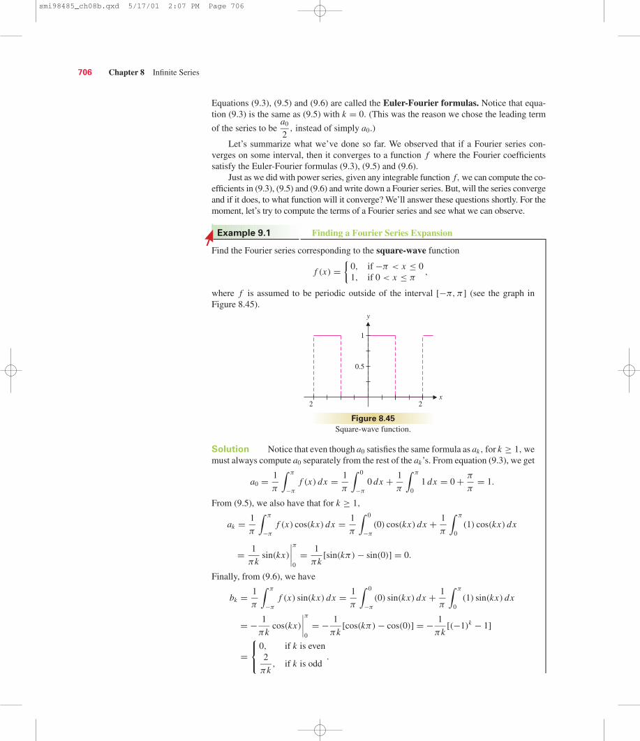
Equations (9.3), (9.5) and (9.6) are called the Euler-Fourier formulas. Notice that equa-tion (9.3) is the same as (9.5) with k = 0. (This was the reason we chose the leading term

of the series to be a0

2, instead of simply a0.)

Let’s summarize what we’ve done so far. We observed that if a Fourier series con-verges on some interval, then it converges to a function f where the Fourier coefficientssatisfy the Euler-Fourier formulas (9.3), (9.5) and (9.6).

Just as we did with power series, given any integrable function f, we can compute the co-efficients in (9.3), (9.5) and (9.6) and write down a Fourier series. But, will the series convergeand if it does, to what function will it converge? We’ll answer these questions shortly. For themoment, let’s try to compute the terms of a Fourier series and see what we can observe.

Find the Fourier series corresponding to the square-wave function

f (x) ={

0, if −π < x ≤ 01, if 0 < x ≤ π

,

where f is assumed to be periodic outside of the interval [−π, π] (see the graph inFigure 8.45).

Solution Notice that even though a0 satisfies the same formula as ak, for k ≥ 1, wemust always compute a0 separately from the rest of the ak’s. From equation (9.3), we get

a0 = 1

π

∫ π

−π

f (x) dx = 1

π

∫ 0

−π

0 dx + 1

π

∫ π

01 dx = 0 + π

π= 1.

From (9.5), we also have that for k ≥ 1,

ak = 1

π

∫ π

−π

f (x) cos(kx) dx = 1

π

∫ 0

−π

(0) cos(kx) dx + 1

π

∫ π

0(1) cos(kx) dx

= 1

πksin(kx)

∣∣∣∣π0

= 1

πk[sin(kπ) − sin(0)] = 0.

Finally, from (9.6), we have

bk = 1

π

∫ π

−π

f (x) sin(kx) dx = 1

π

∫ 0

−π

(0) sin(kx) dx + 1

π

∫ π

0(1) sin(kx) dx

= − 1

πkcos(kx)

∣∣∣∣π0

= − 1

πk[cos(kπ) − cos(0)] = − 1

πk[(−1)k − 1]

=

0, if k is even2

πk, if k is odd

.

Finding a Fourier Series ExpansionExample 9.1


y

x

1

0.5

22

Figure 8.45

Square-wave function.


Notice that we can write the even- and odd-indexed coefficients separately as b2k = 0,

for k = 1, 2, . . . and b2k−1 = 2

(2k − 1)π, for k = 1, 2, . . . . We then have the Fourier

series

a0

2+

∞∑k=1

[ak cos(kx) + bk sin(kx)] = 1

2+

∞∑k=1

bk sin(kx) = 1

2+

∞∑k=1

b2k−1 sin(2k − 1)x

= 1

2+

∞∑k=1

2

(2k − 1)πsin[(2k − 1)x]

= 1

2+ 2

πsin x + 2

3πsin(3x) + 2

5πsin(5x) + · · · .

Notice that none of our existing convergence tests are appropriate for Fourier series.Since we can’t test this, we consider the graphs of the first few partial sums of the seriesdefined by

Fn(x) = 1

2+

n∑k=1

2

(2k − 1)πsin[(2k − 1)x].

In Figures 8.46a–d, we graph a number of these partial sums.

Notice that as n gets larger and larger, the graph of Fn(x) appears to be approaching thegraph of the square-wave function f (x) shown in red and seen in Figure 8.45. Based onthis, we might conjecture that the Fourier series converges to the function f (x). As itturns out, this is not quite correct. We’ll soon see that the series converges to f (x),

everywhere, except at points of discontinuity.

■

Next, we give an example of constructing a Fourier series for another commonwaveform.


y

x

1

0.5

p�p 2p�2p

Figure 8.46d

y = F50(x) and y = f (x).

y

x

1

0.5

p�p 2p�2p

Figure 8.46b

y = F8(x) and y = f (x).

y

x

1

0.5

p�p 2p�2p

Figure 8.46c

y = F20(x) and y = f (x).

y

x

1

0.5

p�p 2p�2p

Figure 8.46a

y = F4(x) and y = f (x).


Find the Fourier series expansion of f (x) = |x |, for −π ≤ x ≤ π, where f is as-sumed to be periodic outside of the interval [−π, π], of period 2π.

Solution In this case, f is the triangular wave function graphed in Figure 8.47.From the Euler-Fourier formulas, we have

a0 = 1

π

∫ π

−π

|x | dx = 1

π

∫ 0

−π

−x dx + 1

π

∫ π

0x dx

= − 1

π

x2

2

∣∣∣∣0

−π

+ 1

π

x2

2

∣∣∣∣π0

= π

2+ π

2= π.

Similarly, for each k ≥ 1, we get

ak = 1

π

∫ π

−π

|x | cos(kx) dx = 1

π

∫ 0

−π

(−x) cos(kx) dx + 1

π

∫ π

0x cos(kx) dx .

Both integrals require the same integration by parts. We let

u = x dv = cos(kx) dx

du = dx v = 1

ksin(kx)

so that

ak = − 1

π

∫ 0

−π

x cos(kx) dx + 1

π

∫ π

0x cos(kx) dx

= − 1

π

[x

ksin(kx)

]0

−π

+ 1

πk

∫ 0

−π

sin(kx) dx + 1

π

[x

ksin(kx)

]π

0

− 1

πk

∫ π

0sin(kx) dx

= − 1

π

[0+ π

ksin(−πk)

]− 1

πk2cos(kx)

∣∣∣∣0

−π

+ 1

π

[π

ksin(πk)−0

]+ 1

πk2cos(kx)

∣∣∣∣π0

= 0− 1

πk2[cos 0−cos(−kπ)]+0+ 1

πk2[cos(kπ)−cos 0]

= 2

πk2[cos(kπ)−1] =

{0, if k is even−4

πk2, if k is odd

.Since cos(kπ) = 1, when k is even and

cos(kπ) = −1, when k is odd.

Since sin πk = 0

and sin(−πk) = 0.

A Fourier Series Expansion for the Triangular Wave FunctionExample 9.2


y

3

2

p 2p�p�2p�3p�4p 3p 4px

Figure 8.47

Triangular wave.


Writing the even- and odd-indexed coefficients separately, we have a2k = 0, for k = 1,

2, . . . and a2k−1 = −4

π(2k − 1)2, for k = 1, 2, . . . . We leave it as an exercise to show that

bk = 0, for all k.

This gives us the Fourier series

a0

2+

∞∑k=1

[ak cos(kx)+bk sin(kx)] = π

2+

∞∑k=1

ak cos(kx) = π

2+

∞∑k=1

a2k−1 cos(2k − 1)x

= π

2−

∞∑k=1

4

π(2k −1)2cos(2k −1)x

= π

2− 4

πcos x − 4

9πcos(3x)− 4

25πcos(5x)−· · · .

You can show that this series converges absolutely for all x, by using the ComparisonTest, since

|ak | =∣∣∣∣ 4

π(2k − 1)2cos(2k − 1)x

∣∣∣∣ ≤ 4

π(2k − 1)2

and the series ∞∑

k=1

4

π(2k − 1)2converges. (Hint: Compare this last series to the conver-

gent p-series ∞∑

k=1

1

k2, using the Limit Comparison Test.) To get an idea of the function

to which the series is converging, we plot several of the partial sums of the series,

Fn(x) = π

2−

n∑k=1

4

π(2k − 1)2cos(2k − 1)x .

See if you can conjecture the sum of the series by looking at Figures 8.48a–d (below andon the following page). Notice how quickly the partial sums of the series appear to con-verge to the triangular wave function f (shown in red; also see Figure 8.47). As it turnsout, the graph of the partial sums will not change appreciably if you plot Fn(x) for muchlarger values of n. (Try this!) We’ll see later how to be sure that the Fourier series con-verges to f (x) for all x . There’s something further to note here: the accuracy of the ap-proximation is fairly uniform. That is, the difference between a given partial sum and fis roughly the same for each x . Take care to distinguish this behavior from that of Taylor


y

3

2


Figure 8.48a

y = F1(x) and y = f (x).

y

3

2


Figure 8.48b

y = F2(x) and y = f (x).


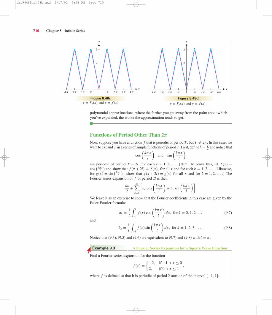
polynomial approximations, where the farther you get away from the point about whichyou’ve expanded, the worse the approximation tends to get.

■

Functions of Period Other Than 2ππ

Now, suppose you have a function f that is periodic of period T, but T �= 2π. In this case, wewant to expand f in a series of simple functions of period T .First, define l = T

2 and notice that

cos

(kπx

l

)and sin

(kπx

l

)are periodic of period T = 2l, for each k = 1, 2, . . . . [Hint: To prove this, let f (x) =cos

(kπx

l

)and show that f (x + 2l) = f (x), for all x and for each k = 1, 2, . . . . Likewise,

for g(x) = sin(

kπxl

), show that g(x + 2l) = g(x) for all x and for k = 1, 2, . . . .] The

Fourier series expansion of f of period 2l is then

a0

2+

∞∑k=1

[ak cos

(kπx

l

)+ bk sin

(kπx

l

)].

We leave it as an exercise to show that the Fourier coefficients in this case are given by theEuler-Fourier formulas:

ak = 1

l

∫ l

−lf (x) cos

(kπx

l

)dx, for k = 0, 1, 2, . . . (9.7)

and

bk = 1

l

∫ l

−lf (x) sin

(kπx

l

)dx, for k = 1, 2, 3, . . . . (9.8)

Notice that (9.3), (9.5) and (9.6) are equivalent to (9.7) and (9.8) with l = π.

Find a Fourier series expansion for the function

f (x) ={−2, if −1 < x ≤ 0

2, if 0 < x ≤ 1,

where f is defined so that it is periodic of period 2 outside of the interval [−1, 1].

A Fourier Series Expansion for a Square Wave FunctionExample 9.3


y

3

2


Figure 8.48c

y = F4(x) and y = f (x).

y

3

2


Figure 8.48d

y = F8(x) and y = f (x).


Solution The graph of f is the square-wave seen in Figure 8.49. From the Euler-Fourier formulas (9.7) and (9.8) with l = 1, we have

a0 = 1

1

∫ 1

−1f (x) dx =

∫ 0

−1(−2) dx +

∫ 1

02 dx = 0.

Likewise, we get

ak = 1

1

∫ 1

−1f (x) cos

(kπx

1

)dx = 0, for k = 1, 2, 3, . . . .

(This is left as an exercise.)

Finally, we have

bk = 1

1

∫ 1

−1f (x) sin

(kπx

1

)dx =

∫ 0

−1(−2) sin(kπx) dx +

∫ 1

02 sin(kπx) dx

= 2

kπcos(kπx)

∣∣∣∣0

−1

− 2

kπcos(kπx)

∣∣∣∣1

0

= 4

kπ[cos 0 − cos(kπ)]

= 4

kπ[1 − cos(kπ)] =

0, if k is even8

kπ, if k is odd

.

This gives us the Fourier series

a0

2+

∞∑k=1

[ak cos(kπx) + bk sin(kπx)] =∞∑

k=1

bk sin(kπx) =∞∑

k=1

b2k−1 sin[(2k − 1)πx]

=∞∑

k=1

8

(2k − 1)πsin[(2k − 1)πx].

Since b2k = 0 and b2k−1 = 8

(2k − 1)π.

Although we as yet have no tools for determining the convergence or divergence of thisseries, we graph a few of the partial sums of the series,

Fn(x) =n∑

k=1

8

(2k − 1)πsin[(2k − 1)πx]

in Figures 8.50a–d (found on the following page). From the graphs, it appears that theseries is converging to the square wave function f, except at the points of discontinuity,x = 0,±1,±2,±3, . . . . At those points, the series appears to converge to 0. You can

Since cos(kπ) = 1, when k is even

and cos(kπ) = −1, when k is odd.


y

x1 2 3�1�2�3

�2

�1

1

2

Figure 8.49

Square wave.


easily verify this by observing that the terms of the series are

8

(2k − 1)πsin[(2k − 1)πx] = 0, for integer values of x .

Since each term in the series is zero, the series converges to 0 at all integer values of x .

You might think of this as follows: at the points where f is discontinuous, the series isconverging to the average of the two function values on either side of the discontinuity.As we will see, this is typical of the convergence of Fourier series.

■

We now state the following major result on the convergence of Fourier series.

Theorem 9.1 (Fourier Convergence Theorem)

Suppose that f is periodic of period 2l and that f and f ′ are continuous on the interval[−l, l], except for at most a finite number of jump discontinuities. Then, f has a con-vergent Fourier series expansion. Further, the series converges to f (x), when f is con-tinuous at x and to

1

2

[lim

t→x+f (t) + lim

t→x−f (t)

]at any points x where f is discontinuous.


y

x1 2 3�1�2�3

�2

�1

1

2

Figure 8.50a

y = F4(x) and y = f (x).

y

x1 2 3�1�2�3

�2

�1

1

2

Figure 8.50b

y = F8(x) and y = f (x).

y

x1 2 3�1�2�3

�2

�1

1

2

Figure 8.50c

y = F20(x) and y = f (x).

y

x1 2 3�1�2�3

�2

�1

1

2

Figure 8.50d

y = F50(x) and y = f (x).


The proof of the theorem is beyond the level of this text and can be found in texts on ad-vanced calculus or Fourier analysis.

■

Use the Fourier Convergence Theorem to prove that the Fourier series expansion ofperiod 2π,

π

2−

∞∑k=1

4

(2k − 1)2πcos(2k − 1)x,

derived in example 9.2, for f (x) = |x |, for −π ≤ x ≤ π and periodic outside of[−π, π], converges to f (x) everywhere.

Solution First, note that f is continuous everywhere (see Figure 8.47). We alsohave that since

f (x) = |x | ={−x, if −π ≤ x < 0

x, if 0 ≤ x < π

and is periodic outside [−π, π], then

f ′(x) ={−1, −π < x < 0

1, 0 < x < π.

So, f ′ is also continuous on [−π, π], except for jump discontinuities at x = 0 andx = ±π. From the Fourier Convergence Theorem, we now have that the Fourier seriesconverges to f everywhere (since f is continuous everywhere). Because of this, we canwrite

f (x) = π

2−

∞∑k=1

4

(2k − 1)2πcos(2k − 1)x,

for all x .

■

As you can see from the Fourier Convergence Theorem, Fourier series do not alwaysconverge to the function you are expanding.

Use the Fourier Convergence Theorem to investigate the convergence of the Fourierseries

∞∑k=1

8

(2k − 1)πsin[(2k − 1)πx],

derived as an expansion of the square-wave function

f (x) ={−2, if −1 < x ≤ 0

2, if 0 < x ≤ 1,

where f is taken to be periodic outside of [−1, 1] (see example 9.3).

Investigating Convergence of a Fourier SeriesExample 9.5

Proving Convergence of a Fourier SeriesExample 9.4

Proof


The Fourier Convergence Theoremsays that a Fourier series may con-verge to a discontinuous function,even though every term in the seriesis continuous (and differentiable) forall x .

Remark 9.1


Solution First, note that f is continuous, except for jump discontinuities at x = 0,±1,±2, . . . . Further,

f ′(x) ={

0, if −1 < x < 00, if 0 < x < 1

and is periodic outside of [−1, 1]. Thus, f ′ is also continuous everywhere, except forjump discontinuities at integer values of x . From the Fourier Convergence Theorem,the Fourier series will converge to f (x) everywhere, except at the discontinuities,x = 0,±1,±2, . . . , where the series converges to the average of the one-sided limits,that is, 0. (Why 0?) Since the series does not converge to f everywhere, we cannot saythat the function and the series are equal. In this case, we usually write

f (x) ∼∞∑

k=1

8

(2k − 1)πsin[(2k − 1)πx]

to indicate that the series corresponds to f (but is not necessarily equal to f ). In the caseof Fourier series, this says that the series converges to f (x) at every x where f is con-tinuous and to the average of the one-sided limits at any jump discontinuities. Noticethat this is the behavior seen in the graphs of the partial sums of the series seen inFigures 8.50a–d.

■

Fourier Series and Music SynthesizersYou may be wondering why we have taken the trouble to investigate Fourier series. Theremust be some significant payoff for all of this work. Most people find it surprising that se-ries of sines and cosines can converge to form line segments, parabolas and other shapes onfinite intervals. As interesting as this is, this is not why we have pursued this study. As itturns out, Fourier series are widely used in engineering, physics, chemistry and so on. Wegive you a sense of how Fourier series are used with the following brief discussion ofmusic synthesizers and a variety of exercises.

Suppose that you had a music machine that could generate pure tones at variouspitches and volumes. What types of sounds could you synthesize by combining severalpure tones together? To answer this question, we first translate the problem into mathemat-ics. A pure tone can be modeled by A sin ωt , where the amplitude A determines the volumeand the frequency ω determines the pitch. For example, to mimic a saxophone, you mustmatch the characteristic waveform of a saxophone (see Figure 8.51). The shape of thewaveform affects the timbre of the tone, a quality most humans readily discern (a saxo-phone sounds different than a trumpet, doesn’t it?).

Consider the following music synthesizer problem. Given a waveform such as the oneshown in Figure 8.51, can you add together several pure tones of the form A sin ωt to ap-proximate the waveform? Note that if the pure tones are of the form b1 sin t , b2 sin 2t ,b3 sin 3t and so on, this is essentially a Fourier series problem. That is, we want to approx-imate a given wave function f (t) by a sum of these pure tones, as follows:

f (t) ≈ b1 sin t + b2 sin 2t + b3 sin 3t + · · · + bn sin nt.

Although the cosine terms are all missing, notice that this is the partial sum of a Fourier se-ries. (Such series are called Fourier sine series and are explored in the exercises.) Formusic synthesizers, the Fourier coefficients are simply the amplitudes of the variousharmonics in a given waveform. In this context, you can think of the bass and treble knobson a stereo as manipulating the amplitudes of different terms in a Fourier series. Cranking


Figure 8.51

Saxophone waveform.


up the bass emphasizes low frequency terms (i.e., increases the coefficients of the first fewterms of the Fourier series), while turning up the treble emphasizes the high frequencyterms. An equalizer (see Figure 8.52) gives you more direct control of individualfrequencies.

In general, the idea of analyzing a wave phenomenon by breaking the wave down intoits component frequencies is essential to much of modern science and engineering. Thistype of spectral analysis is used in numerous scientific disciplines.


Figure 8.52

A graphic equalizer.

EXERCISES 8.9

1. Explain why the Fourier series of f (x) = 1 + 3 cos x −sin 2x on the interval [−π, π] is simply 1 + 3 cos x −

sin 2x . (Hint: Explain what the goal of a Fourier seriesrepresentation is and note that in this case no work needs to bedone.) Would this change if the interval were [−1, 1] instead?

2. Polynomials are built up from the basic operations ofarithmetic. We often use Taylor series to rewrite an

awkward function (e.g., sin x ) into arithmetic form. Many nat-ural phenomena are waves, which are well modeled by sinesand cosines. Discuss the extent to which the following state-ment is true: Fourier series allow us to rewrite algebraic func-tions (e.g., x2) into a natural (wave) form.

3. Theorem 9.1 states that a Fourier series may converge toa function with jump discontinuities. In examples 9.1

and 9.3, identify the locations of the jump discontinuities andthe values to which the Fourier series converges at these points.In what way are these values reasonable compromises?

4. Carefully examine Figures 8.46 and 8.50. For which x’sdoes the Fourier series seem to converge rapidly?

slowly? Note that for every n the partial sum Fn (x) passesexactly through the limiting point for jump discontinuities.Describe the behavior of the partial sums near the jump dis-continuities. This overshoot/undershoot behavior is referred toas the Gibbs phenomenon (see exercise 49 below).

In exercises 5–12, find the Fourier series of the function on the in-terval [−π,π]. Graph the function and the partial sums F4(x)and F8(x) on the interval [−2π, 2π].

5. f (x) = x 6. f (x) = x2

7. f (x) = 2|x | 8. f (x) = 3x

9. f (x) ={

1, if −π < x < 0−1, if 0 < x < π

10. f (x) ={

1, if −π < x < 00, if 0 < x < π

11. f (x) = 3 sin 2x 12. f (x) = 2 sin 3x

In exercises 13–18, find the Fourier series of the function on thegiven interval.

13. f (x) = −x , [−1, 1] 14. f (x) = |x |, [−1, 1]

15. f (x) = x2 , [−1, 1] 16. f (x) = 3x , [−2, 2]

17. f (x) ={

0, if −1 < x < 0x, if 0 < x < 1

18. f (x) ={

0, if −1 < x < 01 − x, if 0 < x < 1

In exercises 19–24, do not compute the Fourier series, but graphthe function to which the Fourier series converges, showing atleast three full periods of the limit function.

19. f (x) = x , [−2, 2] 20. f (x) = x2 , [−3, 3]

21. f (x) ={−x, if −1 < x < 0

0, if 0 < x < 1

22. f (x) ={

1, if −2 < x < 03, if 0 < x < 2

23. f (x) =

−1, if −2 < x < −10, if −1 < x < 11, if 1 < x < 2

24. f (x) =

2, if −2 < x < −1−2, if −1 < x < 10, if 1 < x < 2

25. Substitute x = 1 into the Fourier series formula of exercise 15

to prove that ∞∑

k=1

1

k2= π2

6.

26. Use the Fourier series of example 9.1 to prove that ∞∑

k=1

sin(2k − 1)

(2k − 1)= π

4.


27. Use the Fourier series of example 9.2 to prove that ∞∑

k=1

1

(2k − 1)2= π2

8.

28. Combine the results of exercises 25 and 27 to find ∞∑

k=1

1

(2k)2.

29. You have undoubtedly noticed that many Fourier series consistof only cosine or only sine terms. This can be easily understoodin terms of even and odd functions. A function f (x) is even iff (−x) = f (x) for all x . A function is odd if f (−x) = − f (x)

for all x . Show that cos x is even, sin x is odd and cos x + sin xis neither.

30. If f (x) is even, show that g(x) = f (x) cos x is even andh(x) = f (x) sin x is odd.

31. If f (x) is odd, show that g(x) = f (x) cos x is odd andh(x) = f (x) sin x is even.

32. If f and g are even, what can you say about f g?

33. If f is even and g is odd, what can you say about f g?

34. If f and g are odd, what can you say about f g?

35. Prove the general Euler-Fourier formulas (9.7) and (9.8).

36. If g(x) is an odd function (see exercise 29), show that ∫ l−l g(x) dx = 0 for any (positive) constant l . (Hint: Compare ∫ 0−l g(x) dx and

∫ l0 g(x) dx . You will need to make the change

of variable: t = −x in one of the integrals.) Using the results ofexercise 30, show that if f (x) is even then bk = 0 for all k andthe Fourier series of f (x) consists only of a constant and cosineterms. If f (x) is odd, show that ak = 0 for all k and the Fourierseries of f (x) consists only of sine terms.

In exercises 37–42, use the even/odd properties of f (x) to pre-dict (don’t compute) whether the Fourier series will contain onlycosine, only sine terms or both.

37. f (x) = x3 38. f (x) = x4

39. f (x) = ex 40. f (x) = |x |

41. f (x) ={

0, if −1 < x < 0x, if 0 < x < 1

42. f (x) ={−1, if −2 < x < 0

3, if 0 < x < 2

43. The function f (x) ={−1, if −2 < x < 0

3, if 0 < x < 2is neither even

nor odd, but can be written as f (x) = g(x) + 1 where g(x) ={−2, if −2 < x < 02, if 0 < x < 2

. Explain why the Fourier series of


f (x) will contain sine terms and the constant 1, but no cosineterms.

44. Suppose that you want to find the Fourier series of f (x) =x + x2 . Explain why to find bk you would only need to inte-grate x sin

(kπ x

l

)and to find ak you would only need to inte-

grate x2 cos(

kπ xl

).

Exercises 45–48 are adapted from the owner’s manual of a high-end music synthesizer.

45. A fundamental choice to be made when generating a newtone on a music synthesizer is the waveform. The options aresawtooth, square and pulse. You worked with the sawtooth wavein exercise 13. Graph the limiting function for the function inexercise 13 on the interval [−4, 4]. Explain why “sawtooth’’ isa good name. A square wave is shown in Figure 8.49.A pulse wave of period 2 with width 1/n is generated by

f (x) ={−2, if 1/n < |x | < 1

2, if |x | ≤ 1/n. Graph pulse waves of width

1/3 and 1/4 on the interval [−4, 4].

46. The harmonic content of a wave equals the ratio of integralharmonic waves to the fundamental wave. To understandwhat this means, write the Fourier series of exercise 13 as2π

(sin πx + 1

2 sin 2πx + 13 sin 3πx + 1

4 sin 4πx + · · ·). Theharmonic content of the sawtooth wave is 1

n . Explain how thisrelates to the relative sizes of the Fourier coefficients. The har-monic content of the square wave is 1

n with even-numberedharmonics missing. Compare this description to the Fourier se-ries of example 9.3. The harmonic content of the pulse wave ofwidth 1

3 is 1n with every third harmonic missing. Without com-

puting the Fourier coefficients, write out the general form of the

Fourier series of f (x) ={−2, if 1/3 < |x | < 1

2, if |x | ≤ 1/3.

47. The cutoff frequency setting on a music synthesizer has a dra-matic effect on the timbre of the tone produced. In terms ofharmonic content (see exercise 46), when the cutoff frequencyis set at n > 0, all harmonics beyond the nth harmonic are setequal to 0. In Fourier series terms, explain how this corre-sponds to the partial sum Fn (x). For the sawtooth and squarewaves, graph the waveforms with the cutoff frequency set at 4.Compare these to the waveforms with the cutoff frequency setat 2. As the setting is lowered, you hear more of a “pure’’ tone.Briefly explain why.

48. The resonance setting on a music synthesizer also changes tim-bre significantly. Set at 1, you get the basic waveform (e.g.,sawtooth or square). Set at 2, the harmonic content of the firstfour harmonics are divided by 2, the fifth harmonic is mul-tiplied by 3

4 , the sixth harmonic is left the same, the seventhharmonic is divided by 2 and the remaining harmonics are setto 0. Graph the sawtooth and square waves with resonance set


to 2. Which one is starting to resemble the saxophone wave-form of Figure 8.51?

49. The Gibbs phenomenon is the tendency of approximating par-tial sums of Fourier series to badly undershoot and overshootthe limit function near jump discontinuities (places where thelimit function changes rapidly). A black-and-white photographcan be digitized by partitioning the photograph into small rec-tangles and assigning each rectangle a number. For example, apure white rectangle might be a 1 and a pure black rectangle a10 with grey rectangles assigned values between 1 and 10. Thedigitized photograph can then be approximated by a Fourierseries. A sharp edge in a photograph would have a rapid changefrom black to white, similar to a jump discontinuity. The rapidchange in values from black to white requires high frequencycomponents in the Fourier series (i.e., the terms of the series forlarge values of k). The photograph on the left is out of focus, tothe point that we can’t read the markings on the plane (you canimagine this would be important in many tense situations). Byincreasing the coefficients in the high frequencies in the Fourierseries representation of the photograph, you can get the sharperphotograph on the right. This photograph also has a distinct“halo effect’’ around the plane. Explain how the halo could berelated to the Gibbs phenomenon (photos reprinted by permis-sion from Visualization by Friedhoff and Benzon).

50. Piano tuning is relatively simple due to the phenomenon stud-ied in this exercise. Compare the graphs of sin 8t + sin 8.2t and2 sin 8t . Note especially that the amplitude of sin 8t + sin 8.2tappears to slowly rise and fall. In the trig identity sin 8t +sin 8.2t = [2 cos(0.2t)] sin(8.1t), think of 2 cos(0.2t) as theamplitude of sin(8.1t) and explain why the amplitude variesslowly. Piano tuners often start by striking a tuning fork of acertain pitch (e.g., sin 8t ) and then striking the correspondingpiano note. If the piano is slightly out-of-tune (e.g., sin 8.2t ),the tuning fork plus piano produces a combined tone that no-ticeably increases and decreases in volume. Use your graph toexplain why this occurs.

51. The function sin 8π t represents a 4-Hz signal (1 Hz equals1 cycle per second) if t is measured in seconds. If you receivedthis signal, your task might be to take your measurements of thesignal and try to reconstruct the function. For example, if youmeasured three samples per second, you would have the data


f (0) = 0, f (1/3) = √3/2, f (2/3) = −√

3/2 and f (1) = 0.Knowing the signal is of the form A sin Bt , you would use thedata to try to solve for A and B. In this case, you don’t haveenough information to guarantee getting the right values for Aand B. Prove this by finding several values of A and B withB �= 8π that match the data. A famous result of H. Nyquistfrom 1928 states that to reconstruct a signal of frequency f youneed at least 2 f samples.

52. Suppose that you wanted to approximate a waveformwith sine functions (no cosines), as in the music

synthesizer problem. Such a Fourier sine series will bederived in this exercise. You essentially use Fourier serieswith a trick to guarantee sine terms only. Start with yourwaveform as a function defined on the interval [0, l], forsome length l . Then define a function g(x) that equals f (x) on[0, l] and that is an odd function. Show that g(x) ={

f (x) if 0 ≤ x ≤ l− f (−x) if −l < x < 0

works. Explain why the Fourier

series expansion of g(x) on [−l, l] would contain sine termsonly. This series is the sine series expansion of f (x). Show thefollowing helpful shortcut: the sine series coefficients are

bk = 1

l

∫ l

−lg(x) sin

(kπ

l

)dx = 2

l

∫ l

0f (x) sin

(kπ

l

)dx .

Then compute the sine series expansion of f (x) = x2 on [0, 1]and graph the limit function on [−3, 3].

53. Analogous to exercise 52, develop a Fourier cosineseries and find the cosine series expansion of f (x) = x

on [0, 1].

54. Fourier series is a part of the field of Fourier analy-sis, which is central to many engineering applications.

Fourier analysis includes the Fourier transforms (and the FFTor Fast Fourier Transform) and inverse Fourier transforms,which you will get a brief introduction to in this exercise.Given measurements of a signal (waveform), the goal is toconstruct the Fourier series of a function. To start with asimple version of the problem, suppose the signal has the formf (x) = a0

2 + a1 cos πx + a2 cos 2πx + b1 sin πx + b2 sin 2πxand you have the measurements f (−1) = 0, f

(− 12

) = 1,f (0) = 2, f

(12

) = 1 and f (1) = 0. Substituting into the gen-eral equation for f (x), show that

f (−1) = a0

2− a1 + a2 = 0

f

(−1

2

)= a0

2− a2 − b1 = 1

f (0) = a0

2+ a1 + a2 = 2

f

(1

2

)= a0

2− a2 + b1 = 1

and f (1) = a0

2− a1 + a2 = 0.


Note that the first and last equations are identical and that b2

never appears in an equation. Thus, you have four equationsand four unknowns. Solve the equations. (Hint: Start by com-paring the second and fourth equations, then the third andfifth equations.) You should conclude that f (x) = 1 + cos πx ,with no information about b2 . To determine b2 , we wouldneed another function value. In general, the number of mea-surements determines how many terms you can find in theFourier series (see exercise 51). Fortunately, there is aneasier way of determining the Fourier coefficients. Recall that


ak = ∫ 1−1 f (x) cos nπx dx and bk = ∫ 1

−1 f (x) sin nπx dx . Youcan estimate the integral using function values at x = −1/2,x = 0, x = 1/2 and x = 1. Find a version of a Riemann sumapproximation that gives a0 = 2, a1 = 1, a2 = 0 and b1 = 0.What value is given for b2? Use this Riemann sum rule tofind the appropriate coefficients for the data f

(− 34

) = 34 ,

f(− 1

2

) = 12 , f

(− 14

) = 14 , f (0) = 0, f

(14

) = − 14 , f

(12

) = − 12 ,

f(

34

) = − 34 and f (1) = −1. Compare to the Fourier series of

exercise 13.

C H A P T E R R E V I E W E X E R C I S E S

In exercises 1–8, determine whether the sequence converges ordiverges. If it converges, give the limit.

1. an = 4

3 + n2. an = 3n

1 + n

3. an = (−1)n n

n2 + 44. an = (−1)n n

n + 4

5. an = 4n

n!6. an = n!

nn

7. an = cos πn 8. an = cos nπ

n

In exercises 9–18, answer with “converges” or “diverges” or“can’t tell.”

9. If limk→∞

ak = 1, then ∞∑

k=1

ak .

10. If limk→∞

ak = 0, then ∞∑

k=1

ak .

11. If limk→∞

∣∣∣∣ak+1

ak

∣∣∣∣ = 1, then ∞∑

k=1

ak .

12. If limk→∞

∣∣∣∣ak+1

ak

∣∣∣∣ = 0, then ∞∑

k=1

ak .

13. If limk→∞

ak = 1

2, then

∞∑k=1

ak .

14. If limk→∞

∣∣∣∣ak+1

ak

∣∣∣∣ = 1

2, then

∞∑k=1

ak .

15. If limk→∞

k√

|ak | = 1

2, then

∞∑k=1

ak .

16. If limk→∞

k2ak = 0, then ∞∑

k=1

ak .

17. If p > 1, then ∞∑

k=1

8

k p.

18. If r > 1, then ∞∑

k=1

ark .

In exercises 19–22, find the sum of the convergent series.

19.∞∑

k=0

4

(1

2

)k

20.∞∑

k=1

4

k(k + 2)

21.∞∑

k=0

4−k 22.∞∑

k=0

(−1)k 3

4k

In exercises 23 and 24, estimate the sum of the series to within0.01.

23.∞∑

k=0

(−1)k k

k4 + 124.

∞∑k=0

(−1)k+1 3

k!

In exercises 25–44, determine if the series converges or diverges.

25.∞∑

k=0

2k

k + 326.

∞∑k=0

(−1)k 2k

k + 3


27.∞∑

k=0

(−1)k 4√k + 1

28.∞∑

k=0

4√k + 1

29.∞∑

k=1

3k−7/8 30.∞∑

k=1

2k−8/7

31.∞∑

k=1

√k

k3 + 132.

∞∑k=1

k√k3 + 1

33.∞∑

k=1

(−1)k 4k

k!34.

∞∑k=1

(−1)k 2k

k

35.∞∑

k=1

(−1)k ln

(1 + 1

k

)36.

∞∑k=1

cos kπ√k

37.∞∑

k=1

2

(k + 3)238.

∞∑k=2

4

k ln k

39.∞∑

k=1

k!

3k40.

∞∑k=1

k

3k

41.∞∑

k=1

e1/ k

k242.

∞∑k=1

1

k√

ln k + 1

43.∞∑

k=1

4k

(k!)244.

∞∑k=1

k2 + 4

k3 + 3k + 1

In exercises 45–48, determine if the series converges absolutely,converges conditionally or diverges.

45.∞∑

k=1

(−1)k k

k2 + 146.

∞∑k=1

(−1)k 3

k + 1

47.∞∑

k=1

sin k

k3/248.

∞∑k=1

(−1)k+1 3

ln k + 1

In exercises 49 and 50, find all values of p for which the seriesconverges.

49.∞∑

k=1

2

(3 + k)p50.

∞∑k=1

ek p

In exercises 51 and 52, determine the number of termsnecessary to estimate the sum of the series to within 10−6 .

51.∞∑

k=1

(−1)k 3

k252.

∞∑k=1

(−1)k 2k

k!

In exercises 53–56, find a power series representation for thefunction. Find the radius of convergence.

53.1

4 + x54.

2

6 − x

Chapter Review Exercises 719

55.3

3 + x256.

2

1 + 4x2

In exercises 57 and 58, use the series from exercises 53 and 54 tofind a power series and its radius of convergence.

57. ln(4 + x) 58. ln(6 − x)

In exercises 59–66, find the interval of convergence.

59.∞∑

k=0

(−1)k 2xk 60.∞∑

k=0

(−1)k (2x)k

61.∞∑

k=1

(−1)k 2

kxk 62.

∞∑k=1

−3√k

(x

2

)k

63.∞∑

k=0

4

k!(x − 2)k 64.

∞∑k=0

k2(x + 3)k

65.∞∑

k=0

3k (x − 2)k 66.∞∑

k=0

k

4k(x + 1)k

In exercises 67 and 68, derive the Taylor series of f (x) aboutthe center x = c.

67. f (x) = sin x , c = 0 68. f (x) = 1

x, c = 1

In exercises 69 and 70, find the Taylor polynomial P4(x). Graphf (x) and P4(x).

69. f (x) = ln x , c = 1 70. f (x) = 1√x

, c = 1

In exercises 71 and 72, use the Taylor polynomials fromexercises 69 and 70 to estimate the given values. Determine theorder of the Taylor polynomial needed to estimate the value towithin 10−8 .

71. ln 1.2 72.1√1.1

In exercises 73 and 74, use a known Taylor series to find aTaylor series of the function and find its radius of convergence.

73. e−3x 274. sin 4x

In exercises 75 and 76, use the first five terms of a known Taylorseries to estimate the value of the integral.

75.∫ 1

0tan−1 x dx 76.

∫ 2

0e−3x 2

dx

In exercises 77 and 78, derive the Fourier series of the function.

77. f (x) = x , −2 ≤ x ≤ 2

78. f (x) ={

0 if −π < x ≤ 01 if 0 < x ≤ π


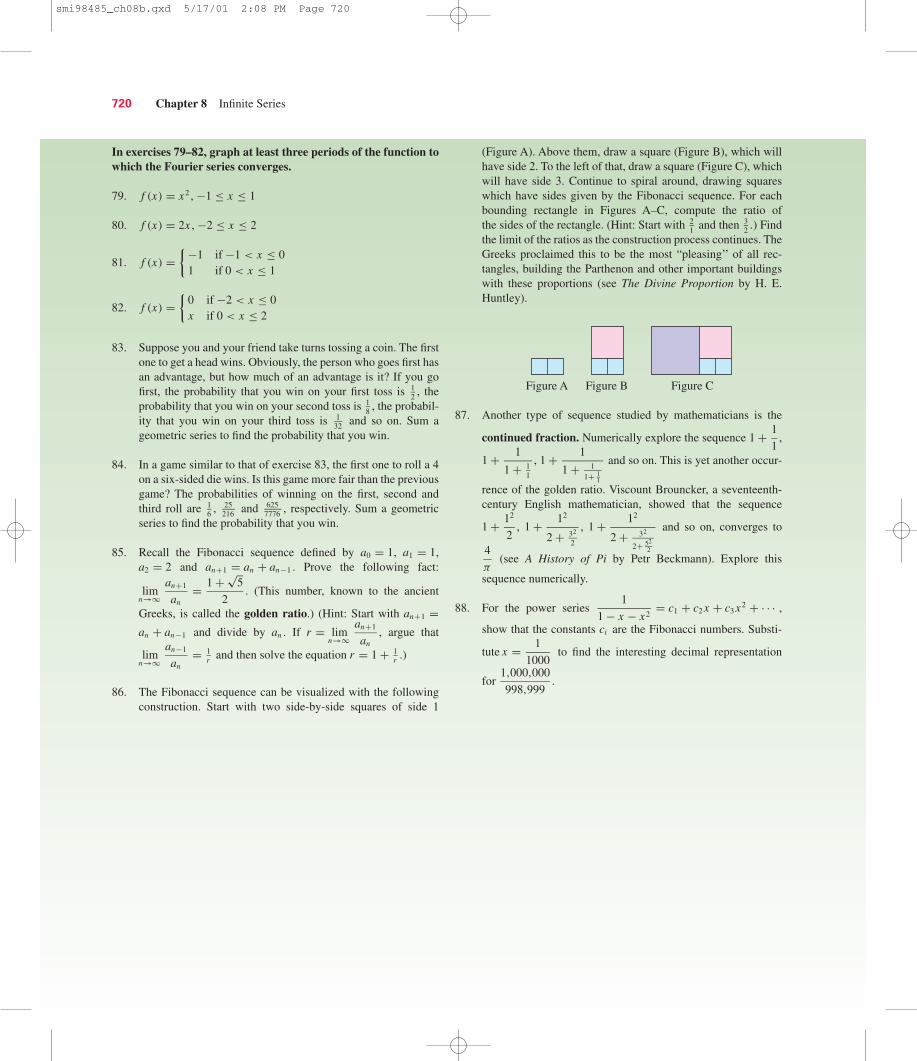
In exercises 79–82, graph at least three periods of the function towhich the Fourier series converges.

79. f (x) = x2 , −1 ≤ x ≤ 1

80. f (x) = 2x , −2 ≤ x ≤ 2

81. f (x) ={−1 if −1 < x ≤ 0

1 if 0 < x ≤ 1

82. f (x) ={

0 if −2 < x ≤ 0x if 0 < x ≤ 2

83. Suppose you and your friend take turns tossing a coin. The firstone to get a head wins. Obviously, the person who goes first hasan advantage, but how much of an advantage is it? If you gofirst, the probability that you win on your first toss is 1

2 , theprobability that you win on your second toss is 1

8 , the probabil-ity that you win on your third toss is 1

32 and so on. Sum ageometric series to find the probability that you win.

84. In a game similar to that of exercise 83, the first one to roll a 4on a six-sided die wins. Is this game more fair than the previousgame? The probabilities of winning on the first, second andthird roll are 1

6 , 25216 and 625

7776 , respectively. Sum a geometricseries to find the probability that you win.

85. Recall the Fibonacci sequence defined by a0 = 1, a1 = 1,a2 = 2 and an+1 = an + an−1 . Prove the following fact:

limn→∞

an+1

an= 1 + √

5

2. (This number, known to the ancient

Greeks, is called the golden ratio.) (Hint: Start with an+1 =an + an−1 and divide by an . If r = lim

n→∞an+1

an, argue that

limn→∞

an−1

an= 1

r and then solve the equation r = 1 + 1r .)

86. The Fibonacci sequence can be visualized with the followingconstruction. Start with two side-by-side squares of side 1


(Figure A). Above them, draw a square (Figure B), which willhave side 2. To the left of that, draw a square (Figure C), whichwill have side 3. Continue to spiral around, drawing squareswhich have sides given by the Fibonacci sequence. For eachbounding rectangle in Figures A–C, compute the ratio ofthe sides of the rectangle. (Hint: Start with 2

1 and then 32 .) Find

the limit of the ratios as the construction process continues. TheGreeks proclaimed this to be the most “pleasing’’ of all rec-tangles, building the Parthenon and other important buildingswith these proportions (see The Divine Proportion by H. E.Huntley).

Figure A Figure B Figure C

87. Another type of sequence studied by mathematicians is the

continued fraction. Numerically explore the sequence 1 + 1

1,

1 + 1

1 + 11

, 1 + 1

1 + 11+ 1

1

and so on. This is yet another occur-

rence of the golden ratio. Viscount Brouncker, a seventeenth-century English mathematician, showed that the sequence

1 + 12

2, 1 + 12

2 + 32

2

, 1 + 12

2 + 32

2+ 522

and so on, converges to

4

π(see A History of Pi by Petr Beckmann). Explore this

sequence numerically.

88. For the power series 1

1 − x − x2= c1 + c2 x + c3 x2 + · · · ,

show that the constants ci are the Fibonacci numbers. Substi-

tute x = 1

1000to find the interesting decimal representation

for 1,000,000

998,999.


8.5 absolute convergence and the ratio … chapter 8 inﬁnite series 8.5 absolute convergence and...

Documents