87a animation of geometric algorithms: a video review

87a

Animation of GeometricAlgorithms: A Video Review

Edited by Marc H. Brown and John Hershberger

June 6, 1992Reformatted for electronic distribution on March 18, 1993

Systems Research Center

DEC’s business and technology objectives require a strong research program. TheSystems Research Center (SRC) and three other research laboratories are commit-ted to filling that need.

SRC began recruiting its first research scientists in l984—their charter, to advancethe state of knowledge in all aspects of computer systems research. Our currentwork includes exploring high-performance personal computing, distributed com-puting, programming environments, system modelling techniques, specification tech-nology, and tightly-coupled multiprocessors.

Our approach to both hardware and software research is to create and use real sys-tems so that we can investigate their properties fully. Complex systems cannot beevaluated solely in the abstract. Based on this belief, our strategy is to demonstratethe technical and practical feasibility of our ideas by building prototypes and usingthem as daily tools. The experience we gain is useful in the short term in enablingus to refine our designs, and invaluable in the long term in helping us to advance thestate of knowledge about those systems. Most of the major advances in informationsystems have come through this strategy, including time-sharing, the ArpaNet, anddistributed personal computing.

SRC also performs work of a more mathematical flavor which complements oursystems research. Some of this work is in established fields of theoretical computerscience, such as the analysis of algorithms, computational geometry, and logics ofprogramming. The rest of this work explores new ground motivated by problemsthat arise in our systems research.

DEC has a strong commitment to communicating the results and experience gainedthrough pursuing these activities. The Company values the improved understand-ing that comes with exposing and testing our ideas within the research community.SRC will therefore report results in conferences, in professional journals, and in ourresearch report series. We will seek users for our prototype systems among thosewith whom we have common research interests, and we will encourage collabora-tion with university researchers.

Robert W. Taylor, Director

Animation of Geometric Algorithms:A Video Review

Edited by Marc H. Brown and John Hershberger

June 6, 1992

Reformatted for electronic distribution on March 18, 1993

iv

c Digital Equipment Corporation 1992

The copyright of each section in this report is held by the author of the section. Sim-ilarly, the copyright of each segment of the accompanying videotape is held by thecontributor of the segment. All other material in the report is copyrighted c DigitalEquipment Corporation 1992. This work may not be copied or reproduced in wholeor in part for any commercial purpose without permission of the authors and indi-vidual contributors.

v

Abstract

Geometric algorithms and data structures are often easiest to understand visually,in terms of the geometric objects they manipulate. Indeed, most papers in compu-tational geometry rely on diagrams to communicate the intuition behind the results.Algorithm animation uses dynamic visual images to explain algorithms. Thus it isnatural to present geometric algorithms, which are inherently dynamic, via algo-rithm animation.

The accompanying videotape presents a video review of geometric animations;the review was premiered at the 1992 ACM Symposium on Computational Geome-try. The video review includes single-algorithm animations and sample graphic dis-plays from “workbench” systems for implementing multiple geometric algorithms.This report contains short descriptions of each video segment.

vi

Preface

This booklet and the accompanying videotape contain animations of a variety ofcomputational geometry algorithms. Computational geometry has existed as a fieldfor almost two decades, and interactive systems for producing algorithm animationshave been available for nearly a decade. A collection like this one is overdue.

The ten segments in this tape cover a wide range of algorithms and represent awide range of software systems. There are animations of fundamental algorithms,such as convex hulls, triangulations, and Voronoi diagrams; there are algorithmsthat helped shape the field in the early and mid-80’s, such as topological sweepand optimal line-segment intersection; and there are recently developed algorithms,such as minimax triangulations. There are single-algorithm animations, general pur-pose algorithm animation systems, and geometric workbenches. There are sequen-tial algorithms and parallel algorithms. And there is some humor.

We received eighteen submissions from fourteen different institutions. We thankthe members of the Video Program Committee for their help in evaluating the en-tries. Besides the editors, the members of the committee were Marshall Bern (XeroxPARC), Leo Guibas (DEC SRC), Jack Snoeyink (University of British Columbia),and Seth Teller (UC Berkeley).

The ten video segments are independent of each other. We suggest that you usethe timings and sequence numbers in the table of contents to view segments of par-ticular interest to you. For example, teachers of introductory computational geome-try courses might find the fundamental algorithms illustrated in segments 2 and 8particularly helpful. Seminars and individual researchers might be more interestedin getting an intuitive look at more recent algorithms in segments such as 1 , 3 ,

and 6 .We believe that algorithm animation has a powerful role to play in communicat-

ing the ideas of geometric algorithms; the accompanying videotape illustrates someof this power. We hope this video review will inspire others to implement and ani-mate their own algorithms, so that animation will become increasingly common incomputational geometry. Most of all, we hope you will enjoy the material as muchas we enjoyed putting it together.

Marc H. BrownJohn Hershberger

vii

Table of Contents

Start Length Title/Author Page

1 1:51 9:42 Real-Time Closest Pairs of Moving Points 1

Simon Kahan

2 11:45 9:06 The XYZ GeoBench:Animation of Geometric Algorithms

5

Peter Schorn, Adrian Brungger,and Michele De Lorenzi

3 21:01 4:47 Optimal Two-Dimensional Triangulations 8

Herbert Edelsbrunner and Roman Waupotitsch

4 25:59 6:33 Boolean Formulae for Simple Polygons 10

John Hershberger and Marc H. Brown

5 32:41 3:46 SHASTRA: A Distributed and CollaborativeDesign Environment

14

Chandrajit L. Bajaj

6 36:36 9:31 Tetrahedral Break-Up 17

Leonidas Palios and Mark Phillips

7 46:15 2:35 Compliant Motion in a Simple Polygon 19

Joseph Friedman

8 49:02 9:17 Workbench for Computational Geometry 22

P. Epstein, J. Kavanagh, A. Knight, J. May,T. Nguyen, and J.-R. Sack

9 58:30 4:16 Topologically Sweeping an Arrangement:A Parallel Implementation

25

Marc H. Brown and Harald Rosenberger

10 1:02:56 11:18 The New Jersey Line-Segment-Saw Massacre 27

Ayellet Tal, Bernard Chazelle, and David Dobkin

Real-Time Closest Pairs of Moving Points

Simon Kahan

Max-Planck Institut fur InformatikSaarbrucken, Germany

1

Tracking moving objects is a fundamental component of many real-time systems ap-plications. This videotape illustrates an algorithm that solves the special case inwhich the number of objects is so large that continual tracking of all objects is im-practical, and an algorithm that computes the closest-pair of point objects.

Overview

Input to the static closest pairs problem is given by the positions of N points in d-space, and output is a list of pairs of points whose distance is minimal over all pairs.In the on-line closest pairs problem, the number of points changes with arbitraryinsertion and deletion operations that, along with closest pair queries, form an inputsequence of requests that must be satisfied upon arrival, with no look-ahead.

In this presentation, we address a real-time closest pair problem. More specifi-cally, our problem falls into the class of Data in Motion problems introduced in [22]and further developed in [23] and [14]. The input is given byN points, just as in thestatic problem, but these points are forever changing with time and correspond topositions of objects external to the physical computational device. Consequently,current positions are not readily available within the computer: instead, each posi-tion is acquired via an explicit update operation per object. Each update is executedas part of the real-time program. An update operation may be viewed as a call toan oracle or sensor that extracts the desired position from the world in which theobjects are moving. In effect, the program chooses its input as a subset of the con-tinuously changing positional data.

1

Companion to video 1 2

Because updates require an excursion from nominal processing, we assume theyconsume a significant amount of real time; certainly far more than that required bya single RAM operation. An important effect is that all real positions are constantlychanging, so those acquired via previous update operations and stored in memorysoon become inaccurate, or stale. In order for the problem to be meaningful, we as-sume that a bound on the maximum rate of positional change is known; thus, stalepositions approximate true positions. In fact, a point must reside within a ball hav-ing radius equal to the product of the rate bound and the time since the point’s lastupdate, and centered about the stale position; the ball is known as the point’s free-range. More general assumptions on positional uncertainty and update costs aredescribed in [21].

The desired output of our real-time closest pair problem is the continual iden-tification of a true closest pair. The output is viewed not as a single discrete entityas in the static problem, nor as a series of separate query responses as in the on-line problem, but instead as a discrete-valued function of real-time. Real-time isdiscretized into frames, each having constant duration.

The goal is to output a function that matches the identity of the true closest pairin as many frames as possible. A major constraint is that updates consume real time,so only a few can be issued per frame. A strategy is needed that chooses these up-dates based on stale data so as to identify the closest pair with as much confidenceas possible. No matter what update strategy is chosen, errors are inevitable in theworst case of all positions nearly coinciding.

The theory of data in motion provides a method for evaluating update strategiesin a framework similar to that just described. Instead of computing the percent-age of errors committed, which may depend on specifics of the object motion, themethod compares (1) the number of updates performed by the strategy before theclosest pair can be correctly deduced from stored data and rate bounds, to (2) theminimal number required in order to prove the answer is correct. Although com-parison by difference is a possibility, the ratio of these two quantities turns out tobe a more convenient performance measure for the closest pairs problem. A strat-egy’s worst case ratio – defined as the maximum over all possible memory config-urations and current positions – is proposed as a good indicator of the strategy’sperformance, and is called the strategy’s lucky ratio. This is analogous to the com-petitive ratio in on-line algorithms theory. The smaller the lucky ratio, the better thestrategy. Or so the theory goes . . .

The accompanying video illustrates three strategies for the closest pair problem:LRU, Greedy, and Pairs. The LRU strategy is to update the least recently updated


position. This is sensible in that it guarantees a minimal upper bound on how stalethe stored positions can become. However, the theory predicts that the LRU strat-egy will perform poorly: its lucky ratio is N , the highest the ratio can ever be.

The Greedy strategy makes use of the known rate bound. It identifies a pairof free-ranges whose boundaries are closest over all pairs, and then updates eitherof the corresponding positions. Since the free-ranges are spheres whose centers arejust the stale positions stored in memory and whose radii are easily computed, iden-tifying the closest pair of free-ranges amounts to the problem of locating the closestpair of spheres. The free-range of the updated position collapses to a point. Theprocess is repeated until the stored positions are sufficient to determine the clos-est pair with certainty. The Pairs strategy is very similar to the Greedy strategy:it differs only in that it updates both positions corresponding to the closest pair offree-ranges. The lucky ratio of the Greedy strategy turns out to be N , just as for theLRU strategy, while the Pairs strategy has a lucky ratio of 2, which is optimal [23].

Besides contradicting our intuition, as explained in the video, there are severalrespects in which the Data in Motion abstraction is an imperfect model of our real-time closest points problem: Lucky ratios are a worst-case measure, and worst-casesituations may occur infrequently in practice. Therefore, a strategy having a smallerlucky ratio might in fact be less efficient in empirical tests. In addition, the ratio isbased on the relative number of updates per query, not the relative number of errorscommitted. Also, the abstraction deals with a single isolated instance of a closestpair query, whereas in the real-time problem the closest pair is to be maintainedat all times: what happens when there is not time to do all the necessary updates?What if the closest pair is obvious with no updates? The former issue may result inerrors; the latter is a matter of implementation: the Greedy and Pairs implementa-tions perform updates in LRU fashion when the closest pair is already determinedbased on stale data.

The software used to produce the simulations in the video is true to the real-time paradigm. Yet the main result – that the Pairs strategy is optimal – jibes withexperiment: in all simulations performed thus far, under a variety of kinds of mo-tion, the most accurate strategy is consistently the Pairs strategy. This corroborationsuggests that the Data in Motion theory is worth consideration when faced with real-time motion problems.


Production Information

The video simulation was created by a C program built upon the Simple RasterGraphics Package (SRGP) available from Brown University and ran on a SUN SPARC-station. The spaghetti source code is available from the author upon request. Film-ing was off the screen via an ordinary camcorder in a dark room. Attempts to di-rectly record the image electronically did not substantially improve the clarity.

Acknowledgments

Thanks to Joan Lawry for help with the frustrating, on-location filming.

The XYZ GeoBench:Animation of Geometric Algorithms

Peter Schorn Adrian Brungger Michele De Lorenzi

Institut fur Theoretische InformatikETH, CH-8092 Zurich

2

This videotape shows the XYZ GeoBench (eXperimental geometrY Zurich) [26, 29,30], a workbench for geometric computation. XYZ GeoBench provides an interac-tive front-end on the Macintosh computer to the XYZ Program Library that containsmany standard algorithms for 2-d problems and some for higher dimensional prob-lems. The execution of all algorithms can be animated.

Contents of the video

The video shows some animations of standard algorithms and a brief demonstrationof the experimental use of the workbench. In particular we show the computation ofthe convex hull, finding a closest pair, and computing all-nearest-neighbors-to-the-left. (An animation of traveling salesman heuristics, alluded to in the video, wasomitted for reasons of length.)

Convex hulls: The first animation shows Graham’s incremental algorithm [17]while the second animation shows Preparata and Hong’s divide and conquer method [27].

Proximity problems: We present a plane sweep for computing the closest-pair [19]and a plane-sweep for computing for each given point a nearest neighbor-to-the-left [20].

Experimenting with the XYZ GeoBench: The final demonstration shows howthe GeoBench can be used interactively to approximate the Voronoi-diagram of a

5


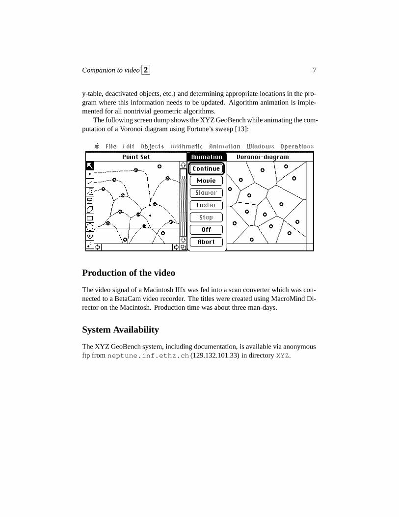
scene of convex objects. The objects (line segments, circles, a hexagon) are enteredusing the mouse, then they are covered with evenly spaced points and the Voronoi-diagram of this point set is computed using Fortune’s sweep [13]. The result givesa good impression of how the Voronoi-diagram of the more complex objects wouldlook like.

Algorithm animation in the XYZ GeoBench

Algorithm animation is used for demonstrating and debugging. We have chosen asimple, yet powerful, approach to animation. There is only one version of an imple-mentation into which code pertaining to the animation is included via conditionalcompilation. This code checks whether animation for this particular algorithm isturned on. If yes, it directly updates the currently visible state of the algorithm andwaits for the user to let it proceed. Finding a graphical representation of a geometri-cal algorithm’s state is usually simple, since geometric objects have standard graph-ical representations. The GeoBench supports the drawing, highlighting and flashingof all geometric objects in a uniform way which lets the implementor easily createanimations. Animation code has the following general structure:

. . .fGeometric algorithm changing internal state.g{$IFC myAlgAnim }fConditional compilation: animation code can be removed easily for higher efficiency.g

if animationFlag[myAlgAnim] then fcheck whether animation is turned ongfUpdate graphical state information, usually draw some objects.gwaitForClick(animationFlag[myAlgAnim]); fdisplay dialog boxgfUpdate graphical state information, usually erase some objects.g

end;{$ENDC }. . .

The procedure waitForClick provides the only interface between the user andthe algorithm currently animated. It supports single step mode and a movie modewith user selectable speed (see the “Animation” dialog box in the screen dump be-low. Updating the visualization of the internal state is facilitated by the conventionthat all drawing on the screen is done using XOR graphics which has the benefitthat erasing is the same as drawing. Animating an algorithm consists of choosinga representation of the internal state (e.g. position of the sweep line, objects in the


y-table, deactivated objects, etc.) and determining appropriate locations in the pro-gram where this information needs to be updated. Algorithm animation is imple-mented for all nontrivial geometric algorithms.

The following screen dump shows the XYZ GeoBench while animating the com-putation of a Voronoi diagram using Fortune’s sweep [13]:

Production of the video

The video signal of a Macintosh IIfx was fed into a scan converter which was con-nected to a BetaCam video recorder. The titles were created using MacroMind Di-rector on the Macintosh. Production time was about three man-days.

System Availability

The XYZ GeoBench system, including documentation, is available via anonymousftp from neptune.inf.ethz.ch (129.132.101.33) in directory XYZ.

Optimal Two-Dimensional Triangulations

Herbert Edelsbrunner Roman Waupotitsch

Department of Computer ScienceUniversity of Illinois at Urbana-Champaign

3

This video illustrates the MINMAXer system. MINMAXer implements various ver-sions of the edge-insertion paradigm for computing optimal two-dimensional trian-gulations. It also includes code for the edge-flip heuristics that can be used to ob-tain locally optimal triangulations. MINMAXer was originally designed for educa-tional purposes and to study the efficiency of algorithms based on the edge-insertionparadigm. It can also be used for a comparative study of the quality achieved byvarious other triangulations introduced in the literature.

Overview

The visual interface offers two main options. First, it allows the user to follow theprogress by showing insertions and deletions of edges in the wire-frame represen-tation. A second option colors the triangles according to their respective measure.With this option one can get a global impression how and how fast the quality ofthe triangulation improves during the iteration.

We briefly review the edge-insertion paradigm. The purpose of the method isto find the triangulation that minimizes the maximum measure over all possible tri-angulations of a given point set. Such measures are for example the largest angleor the slope of a triangle. The algorithm starts with an arbitrary triangulation T anditerates until no improvement is possible. A single iteration adds a new edge to thetriangulation. All edges that intersect this new edge must of course be deleted. Theresulting polygons are now retriangulated. Delicate details of this scheme can befound in [2, 12].

8


The implementation supports the case where the original triangulation containsconstraining edges. Furthermore, it lexicographically optimizes the entire vectorof measures, not just the worst one. Because of this property it usually computes aunique optimum.

For the implementation we use integer arithmetic with ad hoc tie-breaking rules.The triangulations are stored using so the called quadedge data structure. The visualinterface uses the GL graphics library on a Personal Iris Workstation.

Acknowledgments

We thank Ping Fu, Karl Hess, Susan Goode, and Robin Bargar at NCSA for theirhelp in producing this video. The second author thanks Ernst Mucke for his help andadvice concerning the graphics interface. At this point we also like to mention TiowSeng Tan’s contribution who was the first to see that the edge-insertion paradigmcan indeed compute optimal triangulations.

Funding for this research was provided in part by the National Science Foun-dation under grant CCR 89-21421.

Boolean Formulae for Simple Polygons

John Hershberger Marc H. Brown

DEC Systems Research Center130 Lytton Avenue

Palo Alto, CA 94301

4

An animation of an algorithm in action is a powerful tool for exploring the algo-rithm’s behavior. It has proven to be helpful in teaching computer science courses,designing and analyzing algorithms, producing technical drawings, tuning perfor-mance, and documenting programs. As systems for animating algorithms are be-coming more powerful and easier for programmers to use, it is becoming increas-ingly important to identify the techniques that an algorithm animator must use Thisvideo illustrates many of the techniques for algorithm animation reported in the lit-erature thus far [4, 5], especially recent results related to the use of color.

Contents of the video

The algorithm in the videotape finds a representation of a simple polygon’s interioras a monotone Boolean combination of the halfplanes determined by its edges [9].A simple polygon is a closed polygonal path, free of self-intersections; a monotoneBoolean combination is a Boolean formula containing only unions (“+”) and inter-sections (“*”)—no negations are allowed.

The rest of this note itemizes some of the important algorithm animation tech-niques to note while watching the videotape.

Multiple views. It is more effective to illustrate an algorithm with several differentviews than with a single monolithic view. A monolithic view concentrates all the

10


Figure 1

information about an algorithm into one dynamic image. However, to depict a com-plicated algorithm in detail, or multiple aspects of even a simple algorithm, a singlemonolithic view must encode so much information that it quickly becomes difficultfor the user to pick out the details of interest from the wealth of information in theview. Conversely, when each view displays a small number of aspects of the algo-rithm, each view is easy to comprehend in isolation, and the composition of severalviews is more informative than the sum of their individual contributions. The viewsin the figures display the polygon itself, the Boolean formula and its development,and the parse tree corresponding to the formula.

Static history. Especially when animation is used to explain an unfamiliar algo-rithm, it is helpful to present a static view of the history of the algorithm and itsdata structures. Such a view is similar to the way an example might be presentedin a textbook; it allows the user to become familiar with the behavior of the algo-rithm at his own speed, and to focus on the crucial events where significant changeshappen, without paying too much attention to repetitive events.

In Figure 1, the Formula view shows the development of a Boolean formulaover time, as parentheses and operators are added. The CSG Parse Tree view onthe left also embodies a static history: it displays the planar region correspondingto every subformula ever constructed during the algorithm. The Parse Tree view inFigure 2 is a compact version of the same tree that omits the displayed regions.

Amount of input data. It is instructive to introduce an animation on a small prob-lem instance, preferably with textual annotation, to relate the visual displays to theuser’s previous understanding. With small amounts of data, items can be explic-


Figure 2

itly labeled, and the user can easily understand the connections between the views(see Figure 1). Once these connections are established, it is appropriate to introducelarger, more interesting data sets in which the dynamic capabilities of the animationare more fully utilized (see Figure 2). Of course, information such as labels mustbe hidden when displaying these large problem instances, since they would clutterthe view unnecessarily.

Pathological input data. It is often instructive to choose pathological data to pushan algorithm to extreme behavior. For example, in the video the algorithm is runusing both perfectly convex polygons and tight spirals as input. Each input pro-duced a characteristic parse tree (balanced or skewed). When the algorithm is runon less contrived data, we can easily pick out the unbalanced subtrees of the parsetree corresponding to the spirals of the input polygon.

Color unites multiple views. When multiple views show different aspects of thesame data structure, or different representations of logically related objects, an ap-plication can create a smoother, more harmonious picture by painting correspond-ing features with the same colors in all the views. The polygon decomposition an-imation uses the colors blue, red, and black to denote objects that have been, arebeing, or have not yet been processed, respectively. This idea is applied uniformly;combined with the visual prominence of the color red, this makes it easy to see theconnection between the active edges of the polygon and the corresponding activesites in the formula and parse tree views.

Color reveals an algorithm’s state. As mentioned, red, blue, and black are usedto indicate the state of a vertex. In general, as an indicator of algorithm state, color


enhances and complements other techniques in at least three ways. First, it givesan extra dimension for state display—one can encode information in the color ofobjects, as well as in their shape, size, texture, etc. Second, it allows denser pre-sentation of information: fewer pixels are needed to make a color change visiblethan to make a change in the shape of an object visible. Third, color is good fordisplaying global patterns. For example, if a group of small black dots changes to amixture of red and blue dots, it will be much easier to perceive global patterns thanif, say, the circular dots changed to a mixture of black triangles and squares.

Color highlights areas of interest. By temporarily painting a small region with atransparent, contrasting color, an algorithm can focus attention on the painted area.Because the highlight color is transparent, it does not interact visually with the dataelements on the screen, but simply draws the eye to them. A second use of high-lighting is to display transient computations without permanently altering the on-screen state. For example, in Figure 2 (but not in the video), a brown highlightshows a convex hull that is an essential part of the algorithm, but which changestoo rapidly to belong to the relatively stable state displayed in the rest of the view.

Color emphasizes patterns. In Figure 2, each deep subtree in the right view growsdownward at the same time as the highlighted vertex runs inward along one of thespirals in the left view. The colors of the subtrees and the spirals also change in con-cert. The kinetic connection between the two views underlines the linkage betweenspirals and deep parse tree subtrees.

SHASTRA:A Distributed and Collaborative Design

Environment

Chandrajit L. Bajaj

Department of Computer SciencePurdue University

West Lafayette, IN 47907

5

State of the art in Computer Aided Geometric Design (CAGD) is still a single user,single workstation, monolithic environment. At Purdue we are developing a re-search prototype software environment called SHASTRA where multiple users (say,a collaborative engineering design team) create, share, manipulate, simulate, andvisualize complex geometric designs over a distributed network of workstations andsupercomputers.

System Overview

SHASTRA is a highly extensible, collaborative, distributed geometric design andmanipulation environment. At its core is a powerful collaboration substrate to sup-port multi-user applications, and a distribution substrate which emphasizes distributedproblem solving.

Under the umbrella of Project SHASTRA, we have developed software toolkitsGANITH, SHILP and VAIDAK. The GANITH algebraic geometry toolkit manip-ulates polynomial (i.e. algebraic) equations in any number of variables. The SHILPmodeling and display toolkit manipulates curved solid objects with algebraic sur-face boundaries. The VAIDAK medical imaging and model reconstruction toolkitmanipulates medical image volume data.

14


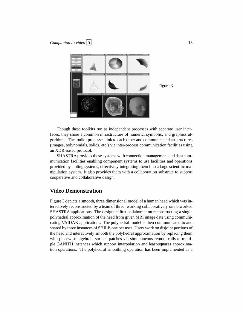
Figure 3

Though these toolkits run as independent processes with separate user inter-faces, they share a common infrastructure of numeric, symbolic, and graphics al-gorithms. The toolkit processes link to each other and communicate data structures(images, polynomials, solids, etc.) via inter-process communication facilities usingan XDR-based protocol.

SHASTRA provides these systems with connection management and data com-munication facilities enabling component systems to use facilities and operationsprovided by sibling systems, effectively integrating them into a large scientific ma-nipulation system. It also provides them with a collaboration substrate to supportcooperative and collaborative design.

Video Demonstration

Figure 3 depicts a smooth, three dimensional model of a human head which was in-teractively reconstructed by a team of three, working collaboratively on networkedSHASTRA applications. The designers first collaborate on reconstructing a singlepolyhedral approximation of the head from given MRI image date using communi-cating VAIDAK applications. The polyhedral model is then communicated to andshared by three instances of SHILP, one per user. Users work on disjoint portions ofthe head and interactively smooth the polyhedral approximation by replacing themwith piecewise algebraic surface patches via simultaneous remote calls to multi-ple GANITH instances which support interpolation and least-squares approxima-tion operations. The polyhedral smoothing operation has been implemented as a


fully distributed algorithm so that a SHILP user can simultaneously instantiate aGANITH process and a remote call, separately for independent faces of the poly-hedral surface. Substantial speedup is obtained for complex designs via this dis-tributed parallelism.

The video shows an animation of the above computation sequence. Note in par-ticular the integration of SHILP, GANITH and VAIDAK.

Implementation Notes

All geometric computations and animation were performed in the SHASTRA dis-tributed and collaborative geometric design environment. The distributed toolkitsof SHASTRA run on any UNIX workstation which support X-11. The animationon the video tape was done using a network of SPARCstations and Personal Irises.Scan conversion from RGB to NTSC and recording on S-VHS tape was achievedby an in-house Panasonic video editing system.

Contributors

The major contributors in the development of the various applications under theSHASTRA umbrella are:

Graduate Students: Vinod Anupam, Steve Cutchin, Jindon Chen, Tamal Dey(Ph.D. August 1991), Insung Ihm (Ph.D. August 1991), Kunihiko Okamura, An-drew Royappa.

Undergraduate Students: Brian Bailey, Andrew Burnett, Daniel Schikore.

Acknowledgments

Funding for this project was provided in part by NSF grants CCR 90-00028, DMS91-01424, AFOSR contract 91-0276, and funds from AT&T and from NSC.

Tetrahedral Break-Up

Leonidas Palios Mark Phillips

The Geometry CenterUniversity of Minnesota

1300 South Second StreetMinneapolis, MN 55454

6

The accompanying videotape contains an animation of an algorithm by Chazelleand Palios to tetrahedralize a nonconvex polyhedron, that is, partition it into tetra-hedra [8].

The Algorithm

The algorithm works in two phases. The goal in the first phase is to reduce the sizeof the polyhedron to be proportional to the number of its reflex edges. To achievethis, we identify vertices whose incident edges all exhibit interior dihedral anglesthat do not exceed �, and remove cone-shaped pieces of the polyhedron with thosevertices as the apexes. As the operation looks very much like pulling a ski hat offsomeone’s head, this phase is called pull-off phase. In the second phase, the fence-off phase, vertical fences are erected through each edge of the polyhedron partition-ing it into cylindrical pieces. Each piece can be defined by (i) specifying a horizon-tal base polygon, (ii) lifting it vertically into an infinite cylinder, and (iii) clippingthe cylinder between two planes (which do not intersect inside the cylinder). Thetriangulation of the base polygons of these pieces and the addition of the verticalfences of the new edges leads to a refined partition into cylindrical pieces whosebases are triangles; each such piece can then be easily decomposed into at most threetetrahedra.

17


The algorithm partitions a polyhedron of n vertices, r reflex edges and zerogenus into O(n+ r

2) tetrahedra, which is asymptotically optimal in the worst case(see [6]). It runs in O((n + r

2) log r) time, and requires O(n + r2) space. In the

process, O(r2) Steiner points are introduced. (Note that the problem of decidingwhether a polyhedron can be partitioned into tetrahedra when no Steiner points areallowed is NP-complete [28].) The computed partition into tetrahedra is not a cellcomplex; the algorithm can, however, be slightly modified to produce a cell com-plex without altering the stated time complexity and size of the partition.

The Animation

The key tool in the production of the animation is Geomview, a general-purpose 3Dviewing program developed at the Geometry Center. Geomview can display geo-metric objects that change under the control of an external program, while allowingthe user to control the viewpoint and other aspects of the display.

The first step in the animation was to use an existing C program which im-plements the described algorithm to decompose the example polyhedron. We thenwrote a C program to choreograph the data; this program generated geometric andmotion description statements which were passed to Geomview via a Unix pipe.The camera location remained under interactive user control which allowed us tofocus on the area of interest without having to program camera motions in advance.


The animation was recorded in real time on a Silicon Graphics VGX workstationwith a Sierra Video Systems RGB to SVHS transcoder to generate video output.

System Availability

Geomview is available on the Internet via anonymous ftp from geom.umn.edu(128.101.25.31). Email inquiries may be sent to [email protected].

Acknowledgments

This work was supported by the National Science Foundation, the Department ofEnergy, Minnesota Technology, Inc., and the University of Minnesota.

Compliant Motion in a Simple Polygon

Joseph Friedman

D. E. Shaw & Co.120 W. 45th Street

New York, NY 10036

7

Compliant motion is a motion paradigm that’s particularly suited for robots withlimited sensing and control uncertainty. Under the simplest variant of the compli-ant motion model, a robot following a commanded direction � travels through freespace in direction � until it encounters an obstacle. Then it slides along the obstacleuntil either friction is too large, or � no longer points into the obstacle. In the for-mer case, it stops; in the latter, it resumes travel through free space in direction �.This type of motion enables the robot to “grope” its way towards the goal [10, 24].

The compliant motion planning problem is that of determining, for a given en-vironment and a starting and goal position, all the commanded directions that cantake a robot from the starting position to the goal (the good directions), if any suchdirections exist.

Overview

This video presents an animation of a compliant motion planning algorithm by Fried-man, Hershberger, and Snoeyink [15]. Given a fixed environment and a goal vertexin the environment, the algorithm analyzes the environment, breaking it up into re-gions. The regions are formed in such a way that all the starting points in the sameregion have similar good directions. This reduces the compliant motion planningproblem to the well-studied point location problem.

When the environment is a fixed simple polygon and the goal is a fixed vertex ofthe environment, the good directions for any starting point form a single interval,

19


bounded by a start direction and a stop direction. We produce two subdivisionsof the environment; we use the start subdivision to determine the start direction,and the stop subdivision for the stop direction. The regions in each subdivision aretriangles and trapezoids.

In order to produce the regions, we work our way backwards from the goal andfollow the changes in the �-backprojection, which is a subset of the environmentcontaining all the starting points for which � is a good direction. As � rotates, the�-backprojection gains and loses regions, and we accumulate these regions in theappropriate subdivision. We compute the regions only for directions � at which the�-backprojection undergoes major changes. Such directions are called events, andcan be attributed to either a vertex or an edge of the environment.

The Video

The video starts with the first phase of the algorithm on a simple polygonal room.The goal is the bottom corner of the room. As the direction � (indicated by the bluearrow in the center) rotates, the bottom copy of the room shows the corresponding�-backprojections. Events are indicated by the flashing edge or vertex that causedthem, and for each event we generate new regions in the start subdivision (the greensubdivision in the top left copy of the room) or the stop subdivision (the red subdi-vision in the top right copy).

When the direction � completes a full turn, the preprocessing is complete, andthe video concludes with three queries for the initial position of the robot. For everyquery point, we consult the start and stop subdivisions for the corresponding boundof the good direction interval, and then we highlight the path followed by a robotcommanded by the middle direction of the good interval to prove that the robot canindeed reach the goal.


We used a Silicon Graphics IRIS 240 GTX workstation to generate the video. Theanimation program is approximately 6,500 lines of C (including an interactive envi-ronment editor), and utilizes Silicon Graphics’ GLTM software. Because of the highrendering speed of the IRIS GTX, we were able to record the video in real time.


Acknowledgments

I wish to thank my friends John Hershberger and Jack Snoeyink, who collaboratedwith me on the compliant motion research. I would also like to thank the followingindividuals from Silicon Graphics for helping with the video. Reuel Nash and JimWinget graciously gave us permission to use SGI facilities. Mike Schulman andTim Heidmann helped with the audio visual equipment.

Workbench for Computational Geometry

P. Epstein J. Kavanagh A. Knight J. May T. NguyenJ.-R. Sack

Computational Geometry Workbench ProjectSchool of Computer ScienceCarleton University, Ottawa

Canada K1S 5B6

8

In this video we illustrate a few of the algorithms that have been developed using ourWorkbench for Computational Geometry. The Workbench is not primarily an algo-rithm animation system, but is designed as a general geometrical programming en-vironment, providing tools for: creating, editing, and manipulating geometric ob-jects; demonstrating and animating geometric algorithms; and most importantly,for implementing and maintaining complex geometric algorithms.

Video Contents

The video first shows several triangulation algorithms. The importance of triangu-lations for a variety of practical applications is well known. In addition to thosesignificant applications, triangulation has become an important tool for other prob-lems in computational geometry. The triangulation algorithms demonstrated are:

� Triangulation via “ear removal”

� Triangulation of monotone polygons [16]

� Triangulation of simple polygons via monotone decomposition [16]

� Triangulation of simple polygons via efficient trapezoidation [33]

22


� Randomized triangulation [31]

The second part of the video shows algorithms based on triangulation. A varietyof problems can be solved in linear time, once a triangulation is known. Amongthese are shortest path problems:

� Point-to-Point Shortest Path [25]

� Shortest Path Tree from a given Point [18]

and link distance problems [32]:

� Construction of window tree

� Execution of a link query

Animation Facilities

In the Workbench, animation of an algorithm is the responsibility of the algorithmimplementor. Code to perform the animation is added, using a simple and well-defined protocol, to the implementation. This approach considerably simplifies theanimation system, but has a cost in flexibility. In particular, the system does notcurrently support different animations of the same algorithm or multiple views inan animation. Animation is simplified considerably by its restriction to the domainof computational geometry. The workbench is an object-oriented system, dealingprimarily with geometric objects that have a clear graphical representation. Manyanimations can be represented by simple manipulations of the same objects used incomputation. This model can easily be extended to arbitrary abstract data types bydefining an appropriate visual representation, but to date our animations are purelygeometric.

The code for animating an algorithm consists mainly of commands to add a“frame” for a particular geometric object or set of objects. These frames are ren-dered and stored as Macintosh PICTs, which improves speed and memory usagefor rendering.

Animating an algorithm usually affects its time and space requirements. Thismust not be allowed to affect algorithms which are not being animated. The work-bench accomplishes this by constructing blocks, unevaluated sections of code, whichare passed to the animation. If animation is not active, these are discarded with avery small constant overhead. If animation is active, they are evaluated to produce


a frame. Thus the same code can be used for animated and non-animated versionswithout modification or recompilation.

A separate process controls display of the animation, allowing animation to besimultaneous with the computation. This process renders each frame as it is sent, aswell as storing it for later replay. The animation process is user-controllable, withcommands modeled after a tape recorder, such as play, record, cue, fast-forward,and stop.

The animation system was designed to allow control of animation depth for al-gorithms which make use of other algorithms as intermediate steps. This is done bymaintaining a hierarchy of animations. When one algorithm calls another, a sub-animation is constructed, containing the animation of the called algorithm. In gen-eral, the result of executing a complex algorithm defines an animation tree. Thedepth of the animation tree defines the depth of the animation. The depth can becontrolled by the user during creation and play-back by using the deeper and shal-lower commands. This allows a user to view execution of an algorithm at an ap-propriate level of detail.

Some algorithms may require interaction with the user during algorithm exe-cution. For example, a shortest path algorithm might ask the user for the sourceand destination of the path. We would expect this request to be made during algo-rithm execution but not during play-back of the animation. The animation systemsupports such input/output interactions.


This video was recorded using a Macintosh II equipped with a NuVista+ video card,whose output was connected directly to a video recorder.

Acknowledgments

This research was partially supported by the Natural Sciences and Engineering Re-search Council of Canada, Carleton University, and the University of Passau.

Topologically Sweeping an Arrangement:A Parallel Implementation

Marc H. Brown Harald Rosenberger

DEC Systems Research Center130 Lytton Avenue

Palo Alto, CA 94301

9

This videotape shows the workings of a topological sweepline, as it visits the O(n2)intersections in an arrangement of n lines in the plane.

Overview

An ordinary sweepline is a vertical line that visits the O(n2) intersections in an ar-rangement of n lines in the plane by sweeping across the arrangement from left toright. Such a sweepline uses only O(n) working storage, but, because it sorts theintersections in x-order, it spendsO(n2 log n) time. In many cases the sorting is un-necessary; it is enough just to visit all the intersections in any order. A topologicalsweepline visits the intersections in optimal O(n2) time by sacrificing the straight-ness of the ordinary sweepline, while retaining the O(n) space bound. [11].

In between visiting intersections, the topological sweepline crosses n edges ofthe arrangement—an upper and a lower edge from each convex face it crosses. Theactive edges—those crossed by the sweepline—are shown in red in the “SweepLine” view. The light blue edges have already been swept, and the thin black edgesremain to be swept. The black dots show intersections that the sweepline could visitnext. The sweepline can choose arbitrarily which black dot to advance over next,or can even advance over all of them in parallel. The lower and upper “Horizon”

25


views display the data structures that the algorithm uses to identify intersections thatit can visit next.

Implementation Notes

The animation was implemented in an in-house dialect of Modula-2 using the Zeusalgorithm animation system [3], and runs on a 5-processor Firefly workstation. De-tails about the techniques used in developing this animation (e.g., the use of colorand the choice of input data) are available elsewhere [4].

The New Jersey Line-Segment-Saw Massacre

Ayellet Tal Bernard Chazelle David Dobkin

Department of Computer SciencePrinceton UniversityPrinceton, NJ 08544

10

This videotape shows a line segment intersection algorithm in action and illustratesits most important features. The algorithm, due to Chazelle and Edelsbrunner [7],has an optimal running time of O(n log n+ k), where n is the number of line seg-ments and k is the number of pairwise intersections.

Overview

As in the classical Bentley-Ottmann method [1], the Chazelle and Edelsbrunner [7]algorithm operates in a sweepline fashion by scanning the segments from left toright, and maintaining the vertical visibility map of the region swept along the way.Two important differences are that (i) the schedule includes only the endpoints ofthe segments and not the intersection points, and (ii) the cross section along thesweepline is maintained in a lazy fashion, meaning that the nodes of the tree rep-resenting the cross section might correspond to segments stranded behind past thesweepline. Also, the loop invariant for the sweepline is not simply that the portionof the map left of it should be maintained but also that the map associated with allthe segments intersecting the sweepline be available as well. Segments are cut upinto smaller pieces in preprocessing, so as to enforce a normalization condition re-lated to the schedule of insertions.

27


Production Notes

The animation comes from a system currently being developed at Princeton by Ayel-let Tal and David Dobkin. This system is intended to ease the interface betweengeometric code and the graphics device. It is built on top of Cheyenne, a device in-dependent graphics library developed by David Dobkin and Eleftheros Koutsofios.The program runs on Sun and Silicon Graphics IRIS workstation. Recording wasdone at the Interactive Computer Graphics Lab at Princeton and editing was donewith the assistance of the Princeton Department of Media Services.

Acknowledgments

This work was supported in part by the National Science Foundation under GrantNumber CCR90–02352.

REFERENCES 29

References

[1] J. L. Bentley and T. A. Ottman. Algorithms for reporting and counting ge-ometric intersections. IEEE Transactions on Computers, C-28(9):643–647,1979.

[2] M. Bern, H. Edelsbrunner, D. Eppstein, S. Mitchel, and T. S. Tan. Edge inser-tion for optimal triangulations. In Proc. 1st Latin American Sympos. Theoret.Informatics, pages 46–60, 1992.

[3] M. H. Brown. Zeus: A system for algorithm animation and multi-view edit-ing. In Proc. IEEE Workshop on Visual Languages, pages 4–9, 1991.

[4] M. H. Brown and J. Hershberger. Color and sound in algorithm animation. InProc. IEEE Workshop on Visual Languages, pages 10–17, 1991.

[5] Marc H. Brown and Robert Sedgewick. Techniques for algorithm animation.IEEE Software, 2(1):28–39, January 1985.

[6] B. Chazelle. Convex partitions of polyhedra: A lower bound and worst-caseoptimal algorithm. SIAM Journal on Computing, 13:488–507, 1984.

[7] B. Chazelle and H. Edelsbrunner. An optimal algorithm for intersecting linesegments in the plane. Journal of the ACM, 39(1):1–54, 1992.

[8] B. Chazelle and L. Palios. Triangulating a nonconvex polytope. Discrete andComputational Geometry, 5:505–526, 1990.

[9] D. Dobkin, L. Guibas, J. Hershberger, and J. Snoeyink. An efficient algorithmfor finding the CSG representation of a simple polygon. Computer Graphics,22(4):31–40, 1988.

[10] B. R. Donald. Error detection and recovery for robot motion planning withuncertainty. Technical Report MIT-AI-TR 982, Artificial Intelligence Labo-ratory, Massachusetts Institute of Technology, 1987.

[11] H. Edelsbrunner and L. J. Guibas. Topologically sweeping an arrangement.J. Comput. System Sci., 38:165–194, 1989.

[12] H. Edelsbrunner, T. S. Tan, and R. Waupotitsch. An O(n2 log n) time algo-rithm for the minmax angle triangulation. In Proc. 6th Ann. Sympos. Comput.Geom., pages 44–52, 1990.

REFERENCES 30

[13] S. Fortune. A sweepline algorithm for Voronoi diagrams. Algorithmica,2:153–174, 1987.

[14] P. G. Franciosa, C. Gaibisso, and M. Talamo. Optimal algorithms for themaxima set problem for data in motion. Technical Report RAP. 03.92, Di-partimento di Informatica e Sistemistica, Universita Degli Studi di Roma “LaSapienza”, February 1992.

[15] J. Friedman, J. Hershberger, and J. Snoeyink. Compliant motion in a simplepolygon. In Proceedings of the 5th ACM Symposium on Computational Ge-ometry, pages 175–186, 1989.

[16] M. R. Garey, D. S. Johnson, F. P. Preparata, and R. E. Tarjan. Triangulating asimple polygon. Inf. Process. Lett., 7(4):175–179, 1978.

[17] R. Graham. An efficient algorithm for determining the convex hull of a finiteplanar set. Information Processing Letters, 1:132–133, 1972.

[18] L. Guibas, J. Hershberger, D. Leven, M. Sharir, and R. Tarjan. Linear timealgorithms for visibility and shortest path problems inside triangulated simplepolygons. Algorithmica, 2:209–233, 1987.

[19] K. Hinrichs, J. Nievergelt, and P. Schorn. Plane-sweep solves the closest pairproblem elegantly. Information Processing Letters, 26:255–261, 1988.

[20] K. Hinrichs, J. Nievergelt, and P. Schorn. An all-round sweep algorithm for2-dimensional nearest-neighbor problems. Acta Informatica, 1990. To appear.

[21] S. H. Kahan. Real-time tracking strategies. In preparation.

[22] S. H. Kahan. A model for data in motion. In Proceedings of the 23rd AnnualACM Symposium on Theory of Computing, 1991.

[23] S. H. Kahan. Real-Time Processing of Moving Data. PhD thesis, Universityof Washington, 1991.

[24] J.-C. Latombe. Robot Motion Planning. The Kluwer international series inengineering and computer science, SECS 0124. Kluwer Academic Publishers,Norwell, Massachusetts, 1991.

[25] D. T. Lee and F. P. Preparata. Euclidean shortest paths in the presence of rec-tilinear barriers. Networks, 14(3):393–410, 1984.

REFERENCES 31

[26] J. Nievergelt, P. Schorn, M. De Lorenzi, C. Ammann, and A. Brungger.XYZ: A project in experimental geometric computation. In Proc. Computa-tional Geometry – Methods, Algorithms and Applications ’91, pages 171–186.Springer, 1991. LNCS 553.

[27] F. Preparata and S. Hong. Convex hulls of finite sets of points in two and threedimensions. Comm. ACM, 20(2):87–93, 1977.

[28] J. Ruppert and R. Seidel. On the difficulty of tetrahedralizing 3-dimensionalnonconvex polyhedra. In Proc. 5th Annual ACM Symposium on Computa-tional Geometry, pages 380–392, 1989.

[29] P. Schorn. Robust Algorithms in a Program Library for Geometric Computa-tion. PhD thesis, ETH, Zurich, Switzerland, 1991.

[30] P. Schorn. The XYZ GeoBench: A programming environment for geometricalgorithms. In Proc. Computational Geometry – Methods, Algorithms andApplications ’91, pages 187–202. Springer, 1991. LNCS 553.

[31] R. Seidel. A simple and fast incremental randomized algorithm for computingtrapezoidal decompositions and for triangulating polygons. Comp. Geom.:Theory and Appl., 1:51–64, 1991.

[32] S. Suri. Minimum Link Paths in Polygons and Related Problems. PhD thesis,The Johns Hopkins University, 1987.

[33] R. E. Tarjan and C. Van Wyk. An O(n log log n)-time algorithm for triangu-lating a simple polygon. SIAM J. Comput., 17:143–178, 1988.

87a animation of geometric algorithms: a video review

Documents