9783642166174 c1

Chapter 3Single Workstation Factory Models

Throughout the analyses given in this textbook, emphasis is on the development ofsteady-state system measures such as the expected number of jobs in the system(WIP) and their mean cycle times (CT ). For these analyses, it is often useful toobtain the probability mass function (pmf) of the steady-state number of jobs inthe system. From these pmf’s, the measures of system effectiveness can often bedeveloped. For notational purposes, define the random variable N as the number ofjobs in the system and define pn as the probability that the number of jobs in thesystem is n; namely, pn = Pr{N = n}. In the first section, a method is developed forderiving equations that determine the steady-state probabilities pn for n = 0,1, · · · .The initial models will include probabilistic behavior for the arrival process andprocessing times, and the early models will restrict these two probability laws to theexponential distribution.

Important assumptions on the operating characteristics of the system are alsomade. It is assumed that job inter-arrival times are independent of the status of thesystem. Another operating assumption is that the server will never be idle whenthere is a job in the system that can be served. That is, if it is allowed for the pro-cessor to serve a job, then no delay occurs between the time that one job leavesthe server and the next job begins processing on the server. Here the assumption ismade that the server is always busy processing jobs when there are jobs availablefor service. Thus, the server will only be idle when there are no jobs available. Inlater models, nonproductive times will be incorporated into the model. For example,in order to have realistic models for many systems, machine breakdowns will needto be incorporated.

3.1 First Model

Consider a single server with a limited waiting area for nmax−1 jobs and one in theserver position for a maximum of nmax jobs in the system. Jobs arrive to the systemone at a time with exponentially distributed inter-arrival times. Denoting the mean

G.L. Curry, R.M. Feldman, Manufacturing Systems Modeling and Analysis, 2nd ed., 69DOI 10.1007/978-3-642-16618-1 3, c© Springer-Verlag Berlin Heidelberg 2011

70 3 Single Workstation Factory Models

arrival rate as λ , the mean inter-arrival time is then 1/λ . If the system is full, thearriving job is rejected (and lost to another factory). If there is room in the waitingarea, the arriving job is accepted and processed in a first-come-first-serve order (thissequence is denoted by FIFO which stands for first-in first-out). The processing timeis also assumed to be exponentially distributed, with mean rate μ (the mean servicetime is 1/μ).

Since this system can have at most nmax jobs, there are nmax + 1 possible states,{0,1, · · · ,nmax}, representing the number of jobs in the system. Interest is in devel-oping the steady-state distribution of the number of jobs in the system. Assumingthat a steady-state exists, then the flow into and out of each state must balance. Thisbalance is the key property used to establish the steady-state probability of being ineach possible system state.

Let pn denote the steady-state probability of n jobs in the system for n =0, · · · ,nmax. The flow into an intermediate state n (0 < n < nmax) is made up oftwo components: (1) the arrival of a new job to the system when the system hasexactly n−1 jobs, and (2) the completion of a job’s service when the system has ex-actly n+1 jobs. The steady-state flow out of an intermediate state n (0 < n < nmax)is also made up of two components: (1) the completion of a job’s service when thesystem has exactly n jobs, and (2) the arrival of a new job to the system when thereare exactly n jobs in the system prior to the arrival event.

The resulting flow balance equation for state n is made up of the above fourcomponents. The mean arrival rate of jobs into the system is λ and the mean servicerate of jobs when there is at least one job in the system is μ . The flow into state noccurs at the rate λ times the probability that the system is in state n− 1 plus therate μ times the probability that the system is in state n + 1. Similarly, the flow outof state n occurs with rate (λ + μ) times the probability that the system is in state n.Thus, the steady-state flow-balance equation for an intermediate state n is

λ pn−1 + μ pn+1 = (λ + μ)pn for n = 1, · · · ,nmax , (3.1)

where the left-hand-side is the inflow and the right-hand-side is the outflow.States 0 and nmax have different equations since some of the terms of the inter-

mediate states equation are not valid for these boundary states. For example, theservice rate is zero if there are no jobs in the system (state 0) nor can the systemreside in state -1 so that an arrival event will put it into state 0. Also if the systemis full (state nmax), then no service from state nmax + 1 can occur and no new jobsare allowed to enter the system. The two special flow-balance equations (for states0 and nmax) are

μ p1 = λ p0 (3.2)

andλ pnmax−1 = μ pnmax . (3.3)

These three equations (namely, 3.1, 3.2, and 3.3) specify nmax + 1 equations con-necting the state probabilities pn. In addition, it is also known that the sum of theseprobabilities must add to one. Thus, there exists the additional equation, called the

3.1 First Model 71

norming equation, written asnmax

∑n=0

pn = 1 . (3.4)

It turns out that the system is over-specified; that is, Eqs. (3.1–3.4) contain moreequations than unknowns. To solve the system, any one of the equations can beomitted except for the norming equation. (The reader is asked to consider this pointfurther in Problem 3.6.) After (arbitrarily) eliminating one equation from the systemcomprised of (3.1–3.3), there will be a total of nmax +1 linear equations in nmax +1unknowns from the system defined by (3.1–3.4).

Given the mean arrival rate λ , the mean service rate μ and a system limit ofnmax, the resulting nmax + 1 linear equations can be solved by standard numericalmethods. If nmax is not large, the equations can be written explicitly and solvedfor the specified values of λ and μ . However, because the system (3.1–3.4) has afairly simple structure, it can be also be solved in general by a recursive substitutionscheme and a closed form solution obtained. Not all systems that we develop inthis text will have a structure leading to a general solution, but when this can beaccomplished, it is the preferred method since the values of the parameters λ , μ andnmax need not be specified and a parametric solution for all values (or acceptableranges of these parameter values) is obtained when solving the general system. Forillustrative purposes, the system (3.1–3.4) is solved by both methods.

Example 3.1. Specific Solution. Consider a facility with a single machine that isused to service only one type of job. The company policy is to limit the number oforders accepted at any one time to 3. The mean arrival rate of orders, λ , is 5 jobsper day, and the mean processing time for a job is 1/4 day (thus, the processingrate is μ = 4/day). Both the processing and inter-arrival times are assumed to beexponentially distributed. These assumptions lead to the system of equations

4p1−5p0 = 0

5p0 +4p2− (5+4)p1 = 0

5p1 +4p3− (5+4)p2 = 0

5p2−4p3 = 0

p0 + p1 + p2 + p3 = 1 .

We ignore the fourth equation and only use the first three equations plus the fifth(norming) equation to obtain

(p0, p1, p2, p3) = (0.173,0.217,0.271,0.339) .

(See the appendix for using Excel to solve linear systems of equations.) The numberof lost jobs per hour (i.e., those arriving to a full system) is given by λ p3 = 5×0.339 = 1.695. The server is idle when the system is empty, so the percentage ofserver idle time is 17.3%. Because the system is at steady-state, the throughput isequal to the number of jobs that enter the system per unit time (those jobs thatactually get into the system, called the effective arrival rate). Thus, throughput rate


equals the arrival rate minus the loss rate; namely, 5 - 1.695 = 3.305 jobs/day. Notethat

WIP = E[N] = ∑npn = 1×0.217+2×0.271+3×0.339 = 1.776 jobs ,

CT = WIP/th = WIP/(λ (1− p3)) = 1.776/3.305 = 0.537 days .

��Example 3.2. General Solution. To illustrate the more general solution approach,this system of equations is solved using the parameters rather than their actual val-ues. The system to be solved is

μ p1−λ p0 = 0

λ p0 + μ p2− (λ + μ)p1 = 0

λ p1 + μ p3− (λ + μ)p2 = 0

λ p2−μ p3 = 0

p0 + p1 + p2 + p3 = 1 .

As before, the first three equations and the fifth equation will be used. The so-lution procedure is a two-step process. First, all variables are expressed in terms ofp0 by use of the first three equations. This is accomplished through a series of suc-cessive substitutions. Second, the value of p0 is obtained by the use of the normingequation. Specifically, the first equation yields p1 in terms of p0 by

μ p1 = λ p0

p1 =λμ

p0 .

The variable p2 is obtained as a function of p0 by substituting the expression for p1

into the second equation as

λ p0 + μ p2 = (λ + μ)p1

μ p2 = (λ + μ)p1−λ p0

p2 = (λ + μ)λμ2 p0− λ

μp0

p2 =(

λμ

)2

p0 .

Similarly, the third equation is used to obtain p3 as a function of p0 by substitutingthe expressions for the previously obtained p1 and p2; namely,

λ p1 + μ p3 = (λ + μ)p2

p3 = (λ + μ)λ 2

μ3 p0−(

λμ

)2

p0

3.2 Diagram Method for Developing the Balance Equations 73

p3 =(

λμ

)3

p0 .

The conclusion from the first step is that all probabilities are now in terms of p0;namely,

p1 =(

λμ

)

p0, p2 =(

λμ

)2

p0, p3 =(

λμ

)3

p0 . (3.5)

The final step is to substitute these expressions into the norming equation as follows:

1 = p0 + p1 + p2 + p3

=

[

1+λμ

+(

λμ

)2

+(

λμ

)3]

p0 = 1

thus

p0 =

[

1+λμ

+(

λμ

)2

+(

λμ

)3]−1

. (3.6)

From here we can develop the measures of WIP = p1 + 2p2 + 3p3, th = λ (p0 +p1 + p2), and CT = WIP/th. ��

Before moving to the remainder of the chapter, it is beneficial to formally definethe effective arrival rate and comment on Little’s Law. Whenever the system is finite,there is the possibility that the system will be full and arriving jobs will be lost;hence, the actual rate of jobs that enter the system, λe may not be the same as thearrival rate, λ .

Definition 3.1. The effective arrival rate for a system is the rate at which jobs enterthe system. For a workstation with constant arrival rate, λ , and with a maximumnumber of jobs at the workstation limited to nmax, the effective arrival rate is givenby

λe = λ (1− pnmax)

where pnmax is the probability that the workstation is full.

A system at steady-state will have its system throughput rate equal to the effectivearrival rate; that is, th = λe, and the use of Little’s Law (Property 2.1) must alwaysuse λe and not λ for the throughput.

• Suggestion: Do Problem 3.1.

3.2 Diagram Method for Developing the Balance Equations

There is a relatively straightforward method for developing the balance equationsfor essentially any system in steady-state whose inter-arrival and service times are


exponentially distributed. The approach is to start by listing all of the states as nodesin a network. For the single-server problem, a sequential listing is the best. As onedevelops an understanding of this approach, a suitable layout will be apparent. Thenode listing is

Now directional arcs are added to the network to represent possible flows be-tween nodes (states). For instance, node 0 is connected to node 1 to represent theflow from state 0 to 1 when an arrival occurs and the system is in state 0. Similarly,node 1 is connected to node 0 to represent the flow when a service occurs with thesystem in state 1 (a service results in an empty system or state 0). States 1 and 2are connected, with a directed arc from 1 to 2, by an arrival event while in state 1.Conversely, states 1 and 2 are connected by a service event while in state 2; thus, thedirected arc is from 2 to 1. The same logic connects states 2 and 3. So the followingdirected network is obtained. Note that an arrival into the system cannot occur whenthe system is in state 3 (i.e., when the system is full).

Now that the appropriately directed arc network of the system being modeled hasbeen developed, the actual flow rates can be displayed on theses arcs. These ratesare relatively straightforward to determine. Since the system has an arrival processthat does not depend on the state of the system (excluding when it is full and so noarrivals can occur), the upward movements among the states all occur at a rate λtimes the probability of being in that state, pn. That is, the conditional arrival rategiven that the system is in state n is λ and the net upward rate from state n is λ pn.The downward movements all occur when a service has been completed and thesehave rates that are μ times the probability of being in the particular state, pn. Thus,the conditional service rate given that there is a job in the system to be serviced isμ . The resulting downward rates from state n is μ pn. The similarity of the servicerates is again due to the assumption about the system. There is a single server andthe service rate is independent of the state of the system. That is, the server worksat the same rate without regard to the number of jobs in the queue. The standardmethod of graphically depicting the flow between states is to label the flow (arrows)with the conditional rates for that state.

μ

λ λ λ

μ μ

3.2 Diagram Method for Developing the Balance Equations 75

This completed directed network can now be used to derive the steady-state bal-ance equations previously analyzed. The logic goes as follows. Partition the nodesinto two subsets of nodes, then establish values for the appropriate steady-state prob-abilities to balance the flow between the two subsets. Partitions are redrawn at n−1different locations to obtain n−1 equations. These balance equations are then com-bined with the norming equations to yield a system of equations similar to the sys-tem of (3.1–3.4).

Consider the two subsets of nodes formed when a cut is made between nodes 0and 1 as is illustrated below.

μ μ

λ λ λ

cut

μ

The balance equation associated with this initial cut is

λ p0 = μ p1 .

The second cut is between states 1 and 2.

μ μ μ

λ λ λ

cut

The resulting balance equation associated with this cut is

λ p1 = μ p2 .

The final cut is between states 2 and 3 as depicted below.

μ μ μ

λ λ λ

cut

Thus the third balance equation is


λ p2 = μ p3 .

These three-balance equations and the norming equation yield another representa-tion for our modeled system as

λ p0 = μ p1

λ p1 = μ p2

λ p2 = μ p3 (3.7)3

∑n=0

pn = 1.

The system (3.7) obviously has the same relationships between the probabilities as(3.1–3.4); however, there is usually less work in obtaining this system using the flowbalance approach. Successive substitution can then be used with (3.7) to obtain (3.5)and the norming equation yields the value for p0 as was accomplished with (3.6).

Another subset partition that leads to the same system of equations is obtainedby separating each node into its own singleton subset. The other subset containsall the other nodes of the network. The associated balance equations for each nodearise when considering the input arcs to the node and balancing those rates withthe outflow arcs. The development of this set of balance equations parallels thediscussion in Sect. 3.1 and is left as an exercise for the reader (Problem 3.2).

The labeled directed arc network and partitioning method is a powerful method-ology for deriving balance equations for queueing systems with exponentially dis-tributed inter-arrival and service times. It is a useful method that helps one visualizethe relationships in the system and keep track of the associated derived balanceequations as they are being developed. Extensive use is made in this textbook of thelabeled-directed arc-diagram approach for studying factory models.

3.3 Model Shorthand Notation

The models studied to this point all assumed exponentially distributed inter-arrivaland service mechanisms. There is a notational shorthand due to Kendall [6] forcharacterizing queueing models that is quite useful. With essentially one word, themodel assumptions and system behavior can be summarized. This notation, or vari-ants of it, frequently appear in the queueing theory literature, particularly in papertitles. This system does not encompass all model variations imaginable, but it doespresent a great deal of information about the system in concise notation. The Kendallnotation for queues is a list of characters each separated by a “/”. The first elementin the list specifies the inter-arrival time distribution assumption. The symbol M (forMarkovian) depicts exponentially distributed times. The second element in the listdenotes the service time distribution assumption. The third element in the list spec-ifies the number of servers and the fourth element is the maximum number of jobs

3.4 An Infinite Capacity Model (M/M/1) 77

allowed in the system at one time. An optional fifth element specifies the assumptionfor the queueing discipline. The general form for Kendall’s notation is

(

arrivalprocess

/

serviceprocess

/

numberof servers

/maximumpossible

in system

/

queuediscipline

)

with Table 3.1 providing a summary of the commonly used abbreviations. Thus, theexample queueing system just studied is denoted as an M/M/1/3 system. The twoserver model of Problem 3.3 is denoted by M/M/2/3. If the system has no effectivelimit on the number of jobs allowed, then the fourth parameter would be infinity.Most often the fourth parameter is omitted when it is not finite, so that such a modelwould often be written as M/M/1 instead of M/M/1/∞.

Table 3.1 Queueing symbols used with Kendall’s notation

Symbols ExplanationM Exponential (Markov) inter-arrival or service timeD Deterministic inter-arrival or service timeEk Erlang type k inter-arrival or service timeG General inter-arrival or service time

1,2, · · · ,∞ Number of parallel servers or capacityFIFO First in, first out queue disciplineLIFO Last in, first out queue disciplineSIRO Service in random orderPRI Priority queue disciplineGD General queue discipline

As the need arises, other parameter designations will be defined such as D for adeterministic time and G for a general distribution. To illustrate this notation, someof the most fundamental results needed for studying factory performance are theG/G/1 model approximations that are taken up at the end of this chapter.

• Suggestion: Do Problems 3.2–3.6.

3.4 An Infinite Capacity Model (M/M/1)

The finite capacity limitation on the M/M/1/3 model just studied is easily dropped,and the removal of this limitation has some interesting consequences. First note thatthe system of equations derived above (i.e., with a finite capacity) has a solutionregardless of the relationship between the arrival rate and the system service rate.If the arrival rate of jobs to the system is larger than the system service capacity,the system is full a relatively high proportion of the time. This in turn leads to morejobs being turned away because of the full system. In fact, the effective arrival rate(those jobs getting into the system) will necessarily be less than the system’s service


capacity. Let’s consider a few cases for the above example that illustrate this point.Suppose that the mean arrival rate is equal to the mean service rate, λ = μ for theM/M/1/3 system. With λ = μ , each probability is equal so that p0 = · · · = p3 =1/4. The effective arrival rate is, thus, given by λe = λ (1− p3) = (3/4)λ < μ . If themean arrival rate is twice the mean service rate, λ = 2μ , then the effective arrivalrate becomes λe = (7/15)λ < μ . For a mean arrival rate that is three times themean service rate, λ = 3μ , the effective arrival rate becomes λe = (13/40)λ < μ .Note that as the ratio of λ/μ becomes larger, the effective arrival rate approachesthe inverse of this ratio but never reaches it. The reader is asked to compute theseeffective rates in Problem 3.5.

One of the lessons to be learned from the finite capacity model is that these sys-tems have a built-in mechanism to adjust the arrival rate (called the effective arrivalrate) to a level that can be handled by the system service capacity. If a system that hasno realistic limit on the number of jobs allowed is considered, then mathematically,these systems can be put in a situation where the mean arrival rate exceeds the meanservice rate and no steady-state exists. It is unreasonable to assume that jobs con-tinue to arrive when there is essentially an infinite queue and the expected cycle timeis also infinite. Of course, one would like to operate well below the blowup pointwith respect to the arrival and service capacity ratio. The analyses of the unlimitedqueueing models result in conditions that establish the existence of the steady-statebehavior for these models.

The formulation of the unlimited-jobs system is very analogous to the finite ca-pacity model formulation. The solution procedure is considerably different in thatan infinite number of states exist and, correspondingly, an infinite number of de-scriptive equations result. Thus, standard numerical solutions for linear equationscannot be used. One is forced to solve these systems in a fashion analogous to theparametric solution approach illustrated for the finite capacity systems. This methodis essentially substitution and formulation of a recursive relationship for the generalsolution structure.

The set of equations for the M/M/1 system is the same as the equations for thefinite system capacity case except that the system does not have a final equation.Thus, an infinite system of equations exists. The diagram for this system is depictedbelow.

21 30 ...

Using the cut partitioning method for obtaining the system of equations neededin defining the steady-state probabilities, the following is obtained:

3.4 An Infinite Capacity Model (M/M/1) 79

λ p0 = μ p1

λ p1 = μ p2

λ p2 = μ p3

...

λ pn = μ pn+1

...∞

∑n=0

pn = 1 .

The above system can be rewritten to obtain the following equivalent system.

p1 = λμ p0

p2 = λμ p1

p3 = λμ p2

...

pn = λμ pn−1

...

Using a successive substitution procedure, each pn term can be written as a functionof p0 to obtain

pn =(

λμ

)n

p0 for n = 0,1, · · · . (3.8)

The final step is to substitute (3.8) into the norming equation yielding

p0 +(

λμ

)

p0 +(

λμ

)2

p0 + · · ·+(

λμ

)n

p0 + · · ·= 1 ,

which can be solved to obtain an expression for p0 as

p0 =1

(

1+ λμ +(

λμ

)2+ · · ·+

(

λμ

)n+ · · ·

) .

The denominator is a geometric series1 that has a finite value if λ/μ < 1. Under thecondition that λ < μ , this series sums to

p0 = 1− λμ

, (3.9)

1 The geometric series is ∑∞n=0 rn = 1/(1− r) for |r|< 1 . Taking the derivative of both sides of the

geometric series yields another useful result, ∑∞n=1 nrn−1 = 1/(1− r)2 for |r|< 1 .


and the general solution to the steady-state probabilities is (given that λ/μ < 1)

pn =(

1− λμ

)(

λμ

)n

for n = 0,1, · · · . (3.10)

The throughput rate per unit time for this system is λ . (The reader is asked to de-velop this result in Problem 3.10.) The utilization factor u for the server is obtainedfrom

u = 0p0 +1

(

∞

∑n=1

pn

)

= 1− p0 = 1−(

1− λμ

)

=λμ

.

The expected number of jobs in the system in steady-state is obtained by using thederivative of the geometric series as follows:

WIPs = E[N] =∞

∑n=0

npn =∞

∑n=0

n

(

1− λμ

)(

λμ

)n

=(

1− λμ

)(

λμ

) ∞

∑n=1

n

(

λμ

)n−1

=(

1− λμ

)(

λμ

)

(

1

1− λμ

)2

=

(

1− λμ

)(

λμ

)

(

1− λμ

)2 =λμ

(

1− λμ

) =u

1−u(3.11)

where N is a random variable denoting the number of jobs in the system. UsingLittle’s Law (Property 2.1), the expected time in system (the cycle time) CTs isgiven by

CTs =WIPs

λ=

1λ

λμ

(1− λμ )

=1

μ−λ. (3.12)

Example 3.3. Consider a single server system with exponentially-distributed inter-arrival times and exponentially-distributed service times (thus, this is an M/M/1system). If 4 jobs per hour arrive for service (λ = 4) and the mean service time is1/5 hour (μ = 5), then the utilization factor u (u = λ/μ) equals 0.8. The expectednumber of jobs in the system, WIPs from (3.11) is

WIPs =0.8

(1−0.8)= 4 .

The cycle time in the system, CTs, is given by (3.12) and is

CTs =1

5−4= 1 hr .

3.5 Multiple Server Systems with Non-identical Service Rates 81

The cycle time in the system is the sum of the cycle time in the queue plus theservice time. Hence, CTq = 1−0.2 = 0.8 hr. The probability that the server is idle,of course, equals the probability that the system is empty, p0. This probability is

p0 = 1− λμ

= 0.2 .

The steady-state probability that there are n jobs in the system is given by

pn = 0.2×0.8n for n = 0,1, · · · .

��A workstation may consist of multiple machines; however, in most models,

server or machine distinctions are not usually made. That is, if there are two ma-chines available, then for ease of modeling it is usually assumed that these are iden-tical machines and that jobs are not split, but processed completely on one machine.Under the assumption of identical machines, if one machine operates at a rate ofμ , then n machines operate at a rate of nμ , and the state diagram must be adjustedaccordingly. For example, suppose a workstation has three machines, then the ser-vice rate when two machines are busy is 2μ and whenever all machines are busy theservice rate is 3μ ; thus, the rate diagram is as below.

21 30 ...

μ 2μ 3μ 3μ


3.5 Multiple Server Systems with Non-identical Service Rates

The assumptions of identical machines may not be accurate, and if there is a sig-nificant difference in the operating characteristics of the machines associated with asingle workstation, more complex models will result. To provide some exposure tothe complexity involved in modeling non-identical machines within a single work-station, a simple non-identical servers model is considered and the associated defin-ing equations for the steady-state probabilities are developed. The structure of thissystem is that it has two non-identical servers and a limit of four jobs in the sys-tem at one time. Inter-arrival and service times are all assumed to be exponentiallydistributed with a mean arrival rate of λ and mean service rates of μ and γ for thetwo distinct machines. Let γ < μ , so that the μ machine is faster and, therefore,


s

f

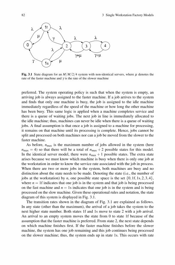
Fig. 3.1 State diagram for an M/M/2/4 system with non-identical servers, where μ denotes therate of the faster machine and γ is the rate of the slower machine

preferred. The system operating policy is such that when the system is empty, anarriving job is always assigned to the faster machine. If a job arrives to the systemand finds that only one machine is busy, the job is assigned to the idle machineimmediately regardless of the speed of the machine or how long the other machinehas been busy. This same logic is applied when a machine completes service andthere is a queue of waiting jobs. The next job in line is immediately allocated tothe idle machine; thus, machines can never be idle when there is a queue of waitingjobs. A final assumption is that once a job is assigned to a machine for processing,it remains on that machine until its processing is complete. Hence, jobs cannot besplit and processed on both machines nor can a job be moved from the slower to thefaster machine.

As before, nmax is the maximum number of jobs allowed in the system (herenmax = 4) so that there will be a total of nmax + 2 possible states for this model.In the identical server model, there were nmax + 1 possible states. The extra statearises because we must know which machine is busy when there is only one job atthe workstation in order to know the service rate associated with the job in process.When there are two or more jobs in the system, both machines are busy and nodistinction about the state needs to be made. Denoting the state (i.e., the number ofjobs at the workstation) by n, one possible state space is the set {0,1f,1s,2,3,4},where n = 1f indicates that one job is in the system and that job is being processedon the fast machine and n = 1s indicates that one job is in the system and is beingprocessed on the slow machine. Given these operational rules and notation, the statediagram of this system is displayed in Fig. 3.1.

The transition rates shown in the diagram of Fig. 3.1 are explained as follows.In any state (other than the maximum), the arrival of a job takes the system to thenext higher state number. Both states 1f and 1s move to state 2 with a job arrival.An arrival to an empty system moves the state from 0 to state 1f because of theassumption that the faster machine is preferred. From state 2, the next state dependson which machine finishes first. If the faster machine finishes before the slowermachine, the system has one job remaining and this job continues being processedon the slower machine; thus, the system ends up in state 1s. This occurs with rate

3.5 Multiple Server Systems with Non-identical Service Rates 83

μ p2. With similar reasoning, it should be clear that if the slower machine completesits processing first, the system transitions to state 1f. The transition from 2 to 1foccurs at a rate of γ p2. Notice that the downward movement from state 2 occurswith rate (μ + γ)p2. Downward movement from state 3 to state 2 occurs with rate(μ + γ)p3 and, similarly, from state 4 to state 3 with rate (μ + γ)p4.

The defining equations for the steady-state probabilities are determined by takingcuts between states. A slight problem exists with defining a cut between states dueto the multiplicity of state 1 (i.e., 1f and 1s). The general idea of a cut is to isolatea set of states from the remaining states. In a serial system this cut process is easilydefined and leads to the number of equations necessary for uniquely defining theprobabilities when combined with the norming equation. The diagram (Fig. 3.1)for this non-identical server system is non-serial and thus there are several morepossibilities for the cuts. The actual cuts that are used in the final analysis must bechosen wisely so that all probabilities are defined. For our set, we shall establish fivecuts such that a cut is placed immediately to the right of each node subset containedwithin the following set:

{ {0},{0,1f},{0,1f,1s},{0,1f,1s,2},{0,1f,1s,2,3} }

thus producing the following five equations:

λ p0 = μ p1f + γ p1sλ p1f = γ p2 + γ p1s

λ p1f +λ p1s = (γ + μ)p2 (3.13)

λ p2 = (γ + μ)p3

λ p3 = (γ + μ)p4 .

These equations, plus the norming equation,

p0 + p1f + p1s + p2 + p3 + p4 = 1

are six equations that can be solved to obtain the steady-state probabilities for thissystem.

Example 3.4. An overhaul facility for helicopters is open 24 hours a day, seven daysa week and helicopters arrive to the facility at an average rate of 3 per day accordingto a Poisson process (i.e., exponential inter-arrival times). One of the areas withinthe facility is for degreasing one of the major components. There is only room in thefacility for 4 jobs at any one time and there are two machines that do the degreasing.The newer of the two degreasing machines takes an average of 8 hours to completethe degreasing and the older machine takes 12 hours for the degreasing operation.Because of the large variability in helicopter conditions, all times are exponentiallydistributed. Thus, we have λ = 3 per day, μ = 3 per day, and γ = 2 per day. Thesystem of equations given by (3.13) become


3p0−3p1f−2p1s = 0

3p1f−2p2−2p1s = 0

3p1f +3p1s−5p2 = 0

3p2−5p3 = 0

3p3−5p4 = 0

p0 + p1f + p1s + p2 + p3 + p4 = 1 .

The solution to this system of equations is

p0 = 0.288, p1f = 0.209, p1s = 0.118, p2 = 0.196, p3 = 0.118, p4 = 0.071 .

The average number in the system is obtained by using the definition of an ex-pected value; namely,

WIPs = p1f + p1s +2p2 +3p3 +4p4 = 1.356

and the average number in the queue is obtained similarly,

WIPq = p3 +2p4 = 0.259 .

Note that for the average number in the queue, p3 is multiplied by 1 because whenthere are 3 in the system, there is only 1 in the queue. Also, p4 is multiplied by2 because when there are 4 in the system, there are 2 in the queue. Average cycletimes are obtained through Little’s Law as

CTs =WIPs

λe=

1.3563× (1−0.071)

= 0.486 day

CTq =WIPq

λe=

0.2593× (1−0.071)

= 0.093 day .

A couple of other measures that are sometimes desired by management are thenumber of busy processors (i.e., degreasers) and their utilization. The expected num-ber of busy servers, E[BS], is 1.097, and is obtained as

E[BS] = 1p1f +1p1s +2p2 +2P3 +2p4 = 1.097 .

The system utilization factor u is the expected number of busy servers divided bythe number of machines available

u =E[BS]

2= 0.5485 = 54.85% .

Our final calculation is to obtain the average time needed for degreasing. Be-cause of the preference given to using the faster machine, we would expect theaverage time to be closer to 8 hours than to 12 hours. To get an exact value, we takeadvantage of the fact that the time in the system equals the time in the queue plus

3.6 Using Exponentials to Approximate General Times 85

service time (Eq. 2.1); thus

E[T ] = CTs−CTq = 0.486−0.093 = 0.393 days = 9.4 hr .

��• Suggestion: Do Problems 3.15–3.20.

3.6 Using Exponentials to Approximate General Times

The exponential distribution is an extremely powerful modeling tool because of itslack of memory (Eq. 1.16 and Problem 1.24). That is, the rate of completion of theprocess does not change with elapsed time. So for systems with exponential times,it is not necessary to keep track of the elapsed inter-arrival time nor the elapsedservice time. This allows the steady-state modeling approach to be used. To modelmore general systems, one fruitful approach is to approximate the general times bycombinations of exponentials. Then the exponential rate modeling approach can stillbe applied by developing more complex state representations of the system.

The Erlang-k distribution (see p. 18 for a review of the Erlang) provides an ex-cellent distribution to use for the expanded state modeling approach. The Erlang-kdistribution is the sum of k independent and identical exponential distributions, sothat it can be modeled as a serial k-node system, with each node referring to iden-tical exponentials. Since the Erlang-k has a squared coefficient of variation givenby C2 = 1/k, it also allows modeling of processes that have less variation than theexponential distribution.

3.6.1 Erlang Processing Times

To illustrate the expanded state modeling approach, consider a single server sys-tem with exponential inter-arrival times having a mean rate λ and a processing timethat is described by an Erlang-2 distribution with mean rate μ and thus mean time1/μ . This Erlang-2 distribution will be modeled using two exponential nodes (orphases), where each node has a mean rate of 2μ . Since rates and times are recipro-cals, the mean time spent in each node is 1/(2μ). This gives the total time spent inthe two nodes as 1/μ (i.e., the sum of the two means) which is equal to the averagetime of the Erlang-2 processing time distribution. To further simplify this example,the number of jobs allowed into the system will be limited to three. Thus, we areinterested in analyzing an M/E2/1/3 system.

The idea of the expanded state space approach is to represent the non-exponentialprocess by more than one node, where each individual node is exponential. There-fore, the service process will have two nodes representing the two phases of theErlang-2 distribution. When a job begins its processing, it enters the node represent-


Fig. 3.2 Diagram for anM/E2/1/3 model where thestate (n, i) indicates that thereare n jobs in the system withthe ith service phase busy

11

12

31

0

21

22 32

ing phase 1 and stays in phase 1 for an exponential length of time. When the job hasbeen completed its phase 1 service, the job moves to the node representing phase 2.As long as the job is in either phase, it is considered to be continuing its processingand a new job is not allowed into service. When the job is finished with phase 2, itis considered to be finished with its processing and it leaves the system, and at thispoint in time, a new job can enter phase 1 to begin its service. A convenient repre-sentation for the state space is to use ordered pairs. In other words, (n, i) denotes astate of the system, where n is the number of jobs in the system and i is the servicephase being occupied by the job being processed. The M/E2/1/3 state diagram isdisplayed in Fig. 3.2.

There are 2nmax + 1 states, where nmax is the maximum number of jobs allowedinto the system (here nmax = 3). To obtain the steady-state probabilities for thissystem, six cuts are placed so that the following node sets are isolated on one sideof the cut

{ {0},{0,(1,2)},{0,(1,1)},{0,(1,1),(1,2)},{(3,1),(3,2)},{(3,2)} }

which together with the norming equation yields the following system of equations,

λ p0−2μ p12 = 0

λ p0 +λ p12−2μ p11 = 0

(λ +2μ)p11−2μ p12−2μ p22 = 0

λ p11 +λ p12−2μ p22 = 0

λ p21 +λ p22−2μ p32 = 0

λ p22 +2μ p31−2μ p32 = 0

p0 + p11 + p12 + p21 + p22 + p31 + p32 = 1 .

The performance measures of work-in-process, cycle time and throughput are com-puted from

WIPs =4

∑n=1

n(pn1 + pn2)

th = λe = λ (1− p31− p32)CTs = WIPs/λe .


3.6.2 Erlang Inter-Arrival Times

If the inter-arrival process is an Erlang distribution then the state-space scheme isslightly different from that used for Erlang service. The same concept of breakingthe service process into phases is used for the arrival process; however, the statespace will be slightly different. We illustrate the expanded state space process ap-plied to arrivals by assuming an Erlang-2 inter-arrival time process. The arrivals willbe processed one-at-a-time at a single workstation with exponentially distributedservice times with a limit of three jobs in the system, in other words, we consider anE2/M/1/3 system.

Conceptually, an arriving job is always in one of two phases, and each phase hasa mean rate of 2λ or a mean sojourn time of 1/(2λ ). As long as a job is in one ofthe arrival phases, it is not yet considered part of the system. The arriving job beginsin phase 1. After an exponentially distributed length of time, the job transitions tophase 2. After another exponential length of time, two events occur simultaneously:the job leaves phase 2 and enters the system and another jobs enters phase 1. (Notethat for a model of phased arrivals, one of the arrival phases is always occupied andthe other phases are empty.)

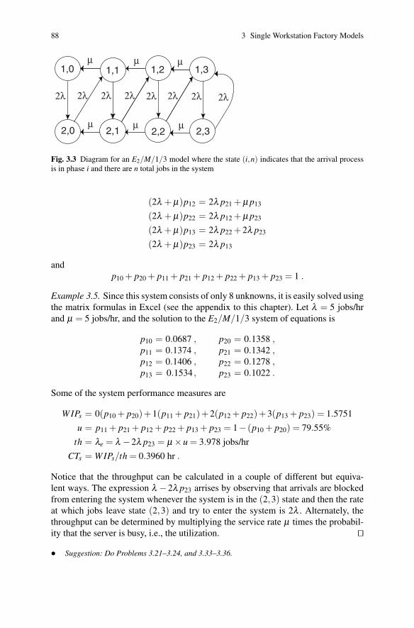
The slight difference in the state space for the Erlang inter-arrival time modelversus the Erlang service time model occurs due to the situation that the arrivalprocess has two phases regardless of the number of jobs in the system. So when thesystem is empty, there are still two phases that the arriving job must complete beforeit becomes an active job attempting to enter the system. The state-space notationused is (i,n) where as before i is the phase and n is the number of jobs in thesystem. Note that the order has been reversed from the Erlang service model to helpkeep in mind that the phases are for the arrival process. The states needed to modelthe E2/M/1/3 system are: {(1,0), (2,0), (1,1), (2,1), (1,2), (2,2), (1,3), (2,3)}. Thediagram of this model is given in Fig. 3.3. Note also that there is a different situationfor blocked jobs for this model. A job is not blocked until it arrives to a full systemwhich occurs from state (2,3) with rate 2λ . Then the arrival process starts over instate (1,3) rather than staying at state (2,3). That is, the arriving job is rejected andthe arrival process starts over at state (1,3) for the next job creation. Thus, there isan arc between (2,3) and (1,3) with rate 2λ in Fig. 3.3 to represent this transition.

Instead of using cuts to derive the equations of state, we use the single-node iso-lation method for generating the equations that define the steady-state probabilities.The following system of equations (all eight equations are given but only seven areused since the norming equation is also required) are generated for the states in theorder that they appear in the above state list.

2λ p10 = μ p11

2λ p20 = 2λ p10 + μ p21

(2λ + μ)p11 = 2λ p20 + μ p12

(2λ + μ)p21 = 2λ p11 + μ p22


1,0μ μ μ

μμ μ

1,1 1,2 1,3

2,0 2,1 2,2 2,3

2λ 2λ 2λ 2λ 2λ 2λ 2λ 2λ

Fig. 3.3 Diagram for an E2/M/1/3 model where the state (i,n) indicates that the arrival processis in phase i and there are n total jobs in the system

(2λ + μ)p12 = 2λ p21 + μ p13

(2λ + μ)p22 = 2λ p12 + μ p23

(2λ + μ)p13 = 2λ p22 +2λ p23

(2λ + μ)p23 = 2λ p13

andp10 + p20 + p11 + p21 + p12 + p22 + p13 + p23 = 1 .

Example 3.5. Since this system consists of only 8 unknowns, it is easily solved usingthe matrix formulas in Excel (see the appendix to this chapter). Let λ = 5 jobs/hrand μ = 5 jobs/hr, and the solution to the E2/M/1/3 system of equations is

p10 = 0.0687 , p20 = 0.1358 ,p11 = 0.1374 , p21 = 0.1342 ,p12 = 0.1406 , p22 = 0.1278 ,p13 = 0.1534 , p23 = 0.1022 .

Some of the system performance measures are

WIPs = 0(p10 + p20)+1(p11 + p21)+2(p12 + p22)+3(p13 + p23) = 1.5751

u = p11 + p21 + p12 + p22 + p13 + p23 = 1− (p10 + p20) = 79.55%

th = λe = λ −2λ p23 = μ×u = 3.978 jobs/hr

CTs = WIPs/th = 0.3960 hr .

Notice that the throughput can be calculated in a couple of different but equiva-lent ways. The expression λ −2λ p23 arrises by observing that arrivals are blockedfrom entering the system whenever the system is in the (2,3) state and then the rateat which jobs leave state (2,3) and try to enter the system is 2λ . Alternately, thethroughput can be determined by multiplying the service rate μ times the probabil-ity that the server is busy, i.e., the utilization. ��• Suggestion: Do Problems 3.21–3.24, and 3.33–3.36.


Fig. 3.4 A generalized Erlangwith two phases, where thefirst phase always occurs andhas a mean rate λ1 and thesecond phase occurs withprobability α and has a meanrate λ2

(1−α) λ2

αλ1

λ1

1 2

3.6.3 Phased Inter-arrival and Processing Times

The improved modeling generality gained from the phased-service time model isfrequently worth the notational inconvenience. For a phased-service time model,the state space is expanded essentially by a multiple of the number of phases. Thestate space for an M/M/1/3 system has four states (nmax + 1), while its extensionto the M/E2/1/3 system has seven states (2nmax +1). The inter-arrival time processcan also be broken into phases at the same time that the service times have phasesto allow for even greater modeling flexibility, and the phases can be structured so asto be more general than the standard Erlang model. To illustrate the approach, theprevious M/E2/1/3 model is extended in this section to have a generalized Erlang-2arrival process. There are two generalizations in the Erlang process that allow for abroader range of squared coefficients of variation, C2, values while maintaining theessential exponential nature of individual nodes. The first generalization is to allowfor non-identical phases and second is to give a probability that the process is com-plete at the end of each phase. Such a phased process is called a Generalized Erlang,GE, or a Coxian distribution. A GE with two phases is diagramed in Fig. 3.4.

A two-phase GE will be denoted by GE2. Thus, the system of interest is anGE2/E2/1/3 model. The purpose of illustrating this generalization is to developmodeling skills that have more flexibility in the range of inter-arrival and servicetime distributions that can be studied. The distribution resulting from the GE2 pro-cess illustrated in Fig. 3.4 can result in a squared coefficient of variation C2 in therange [0.5,∞). Thus, the parameters of an GE2 distribution can be selected to fit anyfinite mean and C2 values needed, given that C2 ≥ 1/2. Notice that we have threeparameters for the GE2 distribution; namely, λ1, λ2, and α . It is possible to fix thosethree parameters to match a given mean, variance, and skewness for a distributionprovided the skewness coefficient is not too large [2, p. 53]. However, it is morecommon to have only the mean and variance for a distribution. Parametric valuesfor the GE2 distribution have been suggested by Altiok [2, p. 54–56] when fittingthe parameters to two moments. These are

λ1 =2

E[X ], λ2 =

1E[X ]C2[X ]

, α =1

2C2[X ]for C2[X ] > 1 ; (3.14)


αλ1 αλ1 αλ1 αλ1

2λ

2λ 2λ 2λ

2μ2μ2μ 2μ 2μ 2μ 2μ

2μ 2μ 2μ 2μ 2μ

(1−α)λ1 (1−α)λ1 (1−α)λ1 (1−α)λ1

2λ 2λαλ1 αλ1 αλ1

(1−α)λ1 (1−α)λ1 2λ (1−α)λ1

Fig. 3.5 State diagram for an GE2/E2/1/3 model, where a (n, i, j) indicates that there are n jobsin the system with one job in arrival phase i and one job is service phase j

λ1 =1

E[X ]C2[X ], λ2 =

2E[X ]

, α = 2(1−C2[X ]) for12≤C2[X ]≤ 1 . (3.15)

Note that matching two parameters of a distribution does not always characterize thedistribution. Some distributions require three or more parameters for proper charac-terization, while the exponential distribution only requires one parameter (the meanrate λ or mean time 1/λ ).

Modeling with the GE2 distribution causes these systems to quickly become quitecomplex. The GE2/E2/1/3 model, illustrated in Fig. 3.5, has 14 states, two statesfor each of the proceeding M/E2/1/3 system states including the 0 state. The sys-tem empty state, state 0, now must be expanded so that the phase of the arrivingjob is represented. As one can readily see from the state diagram (Fig. 3.5) for thissystem, exponential-based generalizations for system times can be accomplished;however, these generalizations yield complex, and often intractable, models. Thenext section develops another approach for approximating general system time dis-tributions (inter-arrival and service times).


3.7 Single Server Model Approximations

There are a variety of single facility generalizations that are standard in the queue-ing literature. Our concern is mainly with the assumptions regarding the inter-arrivaland service time distributions. To use these models in a factory setting, more gen-eral assumptions on these distributions are needed. Rather than giving the generalG/G/1 approximation model directly, a more circumspect route is taken that, hope-fully, illuminates why and where the approximation arose. The model considered

3.7 Single Server Model Approximations 91

next is the exact result for the M/G/1 queue, that in a proper form, suggests thestructure of the general approximation result.

3.7.1 General Service Distributions

Consider a single-server system with exponential inter-arrival times, with mean rateλ , and a general service time distribution having mean time 1/μ and variance σ2

s .The state-diagram approach can no longer be used to develop equations that de-fine the steady-state probabilities since these diagrams are tied to the exponentialdistribution or Markovian property. Variations such as Erlang service times can bedeveloped using the state-diagram approach because the Erlang continues with theexponential assumption for the individual phases. The point of view taken for ageneral service process is to observe the system only at service completion times.This allows us to model, using the Markovian properties of the arrival process, thesteady-state system size probabilities at departure points. It turn out that for thisM/G/1 system, the steady-state probabilities at departure points are the same as thesteady-state probabilities at an arbitrary point in time [4, p. 221]. The derivation ofthese probabilities is beyond the scope of this text and involves developing the gen-erating function transform for the departure point probabilities. The development ofthe mean values for the number of jobs in the system was initially obtained inde-pendently in 1932 by Pollaczek and Khintchine and is now considered a standardproperty for general service time queueing systems.

Property 3.1. The Pollaczek and Khintchine, or “P-K”, formula for WIP inan M/G/1 queueing system is given by

WIPs = E[N] =λμ

+

(

λμ

)2+λ 2σ2

s

2(

1− λμ

)

where N is the number of jobs in the system, λ is the mean arrival rate, and theservice distribution has mean and variance given by 1/μ and σ2

s , respectively.

The notation used in the above property is common throughout this text. The sub-script s used with WIP is to emphasize that the mean work-in-process is over theentire system; the subscript s used with the variance is to emphasize that the param-eter refers to the service time distribution and is frequently used to differentiate theservice distribution parameters from the inter-arrival parameters.

One implication of Little’s Law is that for workstations that have one-at-a-timeprocessing, the relationship between the average number in the system and the aver-age number in the queue is given by WIPs−WIPq = λe/μ . Since λe = λ for M/G/1systems, the expected number of jobs waiting for the processing, E[Nq], is


WIPq = E[Nq] =

(

λμ

)2+λ 2σ2

s

2(

1− λμ

) .

Using Little’s Law one more time, the following important property is obtained, andthis property will be used to develop approximations for more complicated systems.

Property 3.2. The P-K formula for the queue cycle time in an M/G/1 systemis given by

CTq = E[Tq] =WIPq

λ=

(

λμ

)2+λ 2σ2

s

2λ(

1− λμ

)

where Tq is a random variable denoting the time a job spends in the queue, λis the mean arrival rate, and the service distribution has mean and variancegiven by 1/μ and σ2

s , respectively.

The goal is now to rearrange this formula into a form that will be utilized a greatdeal in the development of more realistic factory models. First recall from (1.11)that the squared coefficient of variation is defined by

C2[T ] =V [T ]E[T ]2

so that in terms of service time distribution parameters, we can write

C2s = μ2σ2

s .

Recall from (3.11) and (3.12) that the results for the M/M/1 model are

WIPs(M/M/1) =u

1−u, and

CTs(M/M/1) =1

μ−λ

where u is the server utilization factor and is equal to λ/μ . Here we have introduceda notational convention of writing the model assumptions (i.e., M/M/1) explicitlyin the formula. This convention will be used whenever the context does not makethe model clear. It should not be difficult to show (hint: use (2.1)) the following:

WIPq(M/M/1) =u2

1−u, and

CTq(M/M/1) =u

1−uE[Ts] (3.16)

where Ts is a random variable denoting the time a job spends in the server.


The P-K formula for cycle time in the queue (Property 3.2) can be rewritten as

CTq =

(

λμ

)2+λ 2σ2

s

2λ(

1− λμ

)

=

(

λμ

)2+λ 2 C2

sμ2

2λ(

1− λμ

)

=(

1+C2s

2

) (

u1−u

)

E[Ts] .

Thus, we have an extremely important (exact) relationship between the M/G/1 andthe M/M/1 models; namely,

CTq(M/G/1) =(

1+C2s

2

)

CTq(M/M/1) . (3.17)

3.7.2 Approximations for G/G/1 Systems

The P-K mean queue cycle time result (3.17) is based on the assumption of ex-ponential inter-arrival times. Since the coefficient of variation for the exponentialdistribution is one, the P-K result could just as accurately have been written as

CTq(M/G/1) =(

C2a +C2

s

2

)

CTq(M/M/1) ,

where C2a refers to the squared coefficient of variation for the inter-arrival times.

This form suggests that the relationship might be a reasonable approximation forthe general G/G/1 system. In fact, Kingman [7] looked at various approximationsin heavy-traffic conditions (i.e., for utilization factors close to 1) and obtained asimilar result. Therefore, our first approximation is named after Kingman.

Property 3.3. The Kingman diffusion approximation for the G/G/1 queueingsystem is

CTq(G/G/1)≈(

C2a +C2

s

2

)

CTq(M/M/1) ,

where C2a and C2

s are the squared coefficients of variation for the inter-arrivaldistribution and the service time distribution, respectively.

There have been extensive studies using the Kingman diffusion approximationand it has been shown to be an upper bound on the actual mean queue cycle time.


An improved approximation was developed by Kraemer and Langenbach-Belz [8]and studies by Whitt [10] have shown that it is good when the inter-arrival timevariability is less than the exponential distribution. Whitt’s conclusion is to extendthe approximation by adding another multiplicative term resulting in the following:

CTq(G/G/1)≈ g(u,C2a ,C2

s )×(

C2a +C2

s

2

)

CTq(M/M/1) , (3.18)

where g is a function of server utilization and the two squared coefficients of varia-tion defined as

g(u,C2a ,C2

s ) =

⎧

⎨

⎩

exp{− 2(1−u)3u

(1−C2a)2

C2a+C2

s} for C2

a < 1 ,

1 for C2a ≥ 1 .

For the remainder of this textbook, the simple form of Kingman’s diffusion ap-proximation (Property 3.3) is used with the understanding that improvements arepossible using Whitt’s extension (3.18). Since the time in the system equals the timein the queue plus the processing time, we also have a good approximation for thesystem mean cycle time as

CTs(G/G/1)≈(

C2a +C2

s

2

)(

u1−u

)

E[Ts]+E[Ts] . (3.19)

Example 3.6. Consider again Example 3.3 illustrating an M/M/1 system. For thismodel, λ = 4/hr and μ = 5/hr yielding a utilization factor u = 0.8. Since this wasan exponential system, we had C2

a = C2s = 1 and E[Ts] = 0.2 hr. Thus, the G/G/1

approximation is

CTq(G/G/1) =(

C2a +C2

s

2

)(

u1−u

)

E[Ts] =(

1+12

)(

0.80.2

)

0.2 = 0.8 hr .

Whenever the Kingman approximation (Property 3.3) is applied to an M/M/1 orM/G/1 system, it is exact and not an approximation. We observe that the aboveresult of 0.8 hr for the waiting time agrees exactly with CTq as calculated in Example3.3. (It is always nice to have consistency in mathematics!) ��Example 3.7. Consider a G/G/1 system with inter-arrival times distributed accord-ing to a gamma distribution with mean 15 minutes and standard deviation 30 min-utes, and with service times distributed according to an Erlang-4 distribution withmean 12 minutes. Since the distribution of service times is Erlang, the initial temp-tation may be to use the methodology of Sect. 3.6.1; however, because the arrivaltimes are not exponential, we are left with the G/G/1 results. The given data yieldsthe following parameters: λ = 4/hr, μ = 5/hr, C2

a = 4, and C2s = 0.25. Thus, this

example has the same mean characteristics of Example 3.6 yielding a utilization ofu = 0.8, but the arrival process has more variability and the processing times areless variable. Using the Kingman diffusion approximation (Property 3.3), we have


CTq(G/G/1)≈(

C2a +C2

s

2

)(

u1−u

)

E[Ts] =(

4+0.252

)(

0.80.2

)

0.2 = 1.7 hr .

This cycle time is over twice a large as the exponentially distributed system result;thus, the variability associated with non-exponential distributions can have a signif-icant impact on the expected cycle time.

The queue waiting times for single-server queueing systems can be easily sim-ulated with a spreadsheet model (see the Appendix); thus to check the accuracy ofthe approximation, we simulated the G/G/1 system using Excel as discussed in theappendix. (Also refer to the appendix for the importance of reporting confidence in-tervals along with simulation results.) The simulation yielded a mean waiting timeof 1.89 hours with a half-width of ±2 minutes for the 95% confidence interval. It isinteresting that when a Weibull distribution with the same mean and variance wasused instead of the Gamma distribution, the simulated mean waiting time was 1.71hours with a half width of ±1.5 minutes for the 95% confidence interval. ��

3.7.3 Approximations for G/G/c Systems

There are many generalizations of the G/G/1 approximations to account for multi-ple server systems in the literature. Allen and Cunneen [1] have one of the first com-monly used approximation based on the Kingman diffusion approximation. Theirapproximation was later adjusted by Hall [3] to be a simple extension of Property3.3 and is given as

CTq(G/G/c)≈(

C2a +C2

s

2

)

CTq(M/M/c) . (3.20)

This form of the multiple server approximation is particularly appealing and will beused herein since it reduces to the form of the single-server approximation when c =1. In addition, it is not too difficult to obtain WIP and CT for an M/M/2 system (seeProblem 3.9) and the M/M/3 system; thus, we have the following two properties.

Property 3.4. The Kingman diffusion approximation extended for a two-server system is

CTq(G/G/2)≈(

C2a +C2

s

2

)(

u1−u

)(

u1+u

)

E[Ts] ,

where u = λE[Ts]/2 is server utilization. This approximation is exact for theM/M/2 system.


Property 3.5. The Kingman diffusion approximation extended for a three-server system is

CTq(G/G/3)≈(

C2a +C2

s

2

)(

u1−u

)(

3u2

2+4u+3u2

)

E[Ts] ,

where u = λE[Ts]/3 is server utilization. This approximation is exact for theM/M/3 system.

An approximation proposed in Hopp and Spearman [5] uses the following ap-proximation for a Markovian multiple server system from [9]

CTq(M/M/c) =

(

u√

2c+2−2

c

)

CTq(M/M/1) .

The resulting approximation of Hopp and Spearman yields a general extension as:

Property 3.6. The Kingman diffusion approximation extended for a multi-server system is

CTq(G/G/c)≈(

C2a +C2

s

2

)

(

u√

2c+2−1

c(1−u)

)

E[Ts] ,

where u = λE[Ts]/c is server utilization.

Finally, we repeat the obvious rule for system cycle time (3.19) extended to amultiple-server system that holds whenever service is one-at-a-time:

CTs(G/G/c) = CTq(G/G/c)+E[Ts] . (3.21)

Example 3.8. Consider again the system of Example 3.7 except for a two-serversystem and with a mean service time of 24 minutes. Thus, server utilization staysthe same (namely, u = 0.8) and the squared coefficients of variation are still given asC2

a = 4 and C2s = 0.25. Then the expected system cycle time using the approximation

of Property 3.6 is

CTq(G/G/2) ≈(

4+0.252

)

(

(0.8)√

6−1

2(1−0.8)

)

0.4

= 1.54 hr .

If we use Property 3.4, the approximation becomes

Appendix 97

CTq(G/G/2) ≈(

4+0.252

)(

0.81−0.8

)(

0.81+0.8

)

0.4

= 1.51 hr .

A simulation of this system yielded a mean cycle time in the queue of 1.63 hr witha half-width of ±0.01 hr for the 95% confidence interval. ��

A comparison of the analytical result and the simulation result in the above ex-ample illustrates that these approximations are adequate but certainly not exact.Throughout the next four chapters, we will utilize these approximations extensivelyas we build approximations for more general factory models.


Appendix

In this appendix, we discuss using Excel to solve linear systems of equations andthe use of confidence intervals within a simulation. We also present a very sim-ple method for simulating a single-server queueing system with a FIFO queueingdiscipline.

Solutions to Linear Systems of Equations. Linear systems can always be writ-ten in matrix form as

Ax = b ,

where A is an m× n matrix of the coefficients, x is a vector of n unknowns, and bis an m dimensioned vector of the right-hand-side constants. If the system has thesame number of equations as unknowns (namely, m = n) and if the matrix A has aninverse, the solution to this system is

x = A−1b ,

where A−1 denotes the inverse of the matrix. Excel has functions for both thematrix inverse and for matrix multiplication. The key to using an Excel functionthat has an array for the answer, is to highlight the area of the answer and use<ctrl-shift-enter> when executing the function. For example, suppose wewish to solve the following system:

3x1 +4x2 +5x3 = 4

2x1 +2x2 +5x3 = 3

1x1 +6x2−2x3 = 1 .

Using Excel, type the coefficient matrix, A, in the square block of cells A2:C4 andthe right-hand-side vector in a single column block of cells E2:E4 as shown below.


A B C D E1 Coefficient Matrix RHS2 3 4 5 43 2 2 5 34 1 6 -2 1

The solution to the system, namely A−1b is a 3× 1 array; therefore, a columnof three cells for storing the answer must be selected (highlighted). Choosing thecells G2:G4 for the answer, select those three cells by placing the mouse in cell G2and dragging the mouse down three cells. While the three cells are highlighted, typethe following (the typing will be appear in cell G2 since that is where the selectionstarted)

=MMULT(MINVERSE(A2:C4),E2:E4)

but do not hit the <enter> key. Note that the MMULT() function multiplies twoarrays, and the MINVERSE() function produces the inverse of an array. In Excel,matrix functions always begin with the letter M. When finished typing, hold downthe <ctrl> and <shift> keys and while holding these two key down, hit the<enter> key. The answer (0.75, 0.125, 0.25) should appear in the highlightedcells G2:G4.

Simulation of Waiting Times in a Single-Server Workstation. Consider aG/G/1 queueing system in which each job is numbered sequentially as it arrives.Let the service time of the nth job be denoted by the random variable Sn, the delaytime (time spent in the queue) by the random variable Dn, and the inter-arrival timebetween the n-1st and nth job by the random variable An. The delay time of the nth

job must equal the delay time of the previous job, plus the previous job’s servicetime, minus the inter-arrival time; however, if inter-arrival time is larger than theprevious job’s delay time plus service time, then the queueing delay will be zero. Inother words, the following must hold

Dn = max{0, Dn−1 +Sn−1−An } . (3.22)

If we can generate observations of the random variables An and Sn for n =1, · · · ,nmax we will have simulated the arrival and service times for nmax jobs andthus be able to simulate their delays using (3.22). In the Appendix of Chap. 2, theExcel function RAND() was used to generate random numbers which are defined asa sequence of numbers appearing to have a continuous uniform distribution between0 and 1. General random variates can be obtained by the following property that isused to relate random numbers to any other random variable.

Property 3.7. Let R be a random variable with a continuous uniform distri-bution between zero and one, and let F be an arbitrary CDF. If the inverse ofthe function F exists, denote it by F−1; otherwise, let F−1(a) = min{t|F(t)≥a}. Then the random variable X defined by

X = F−1(R),

Appendix 99

has a distribution function given by F; that is,

P{X ≤ a}= F(a) for −∞ < a < ∞.

To illustrate the use of this property, consider the Excel function

GAMMAINV(probability, shape parameter, scale parameter)

that yields the inverse of the gamma CDF evaluated at the specified probability withthe given shape, α , and scale, β , parameters (review p. 19); thus,

=GAMMAINV(RAND(),4,3)

will generate gamma random variates with mean 12 and standard deviation 6 (be-cause the mean is the shape times scale and the variance is shape times scalesquared).

To begin a simulation of Example 3.7, type the following in the first three rowsof an Excel spreadsheet.

A B C1 InterArrive Service Delay2 0 =GAMMAINV(RAND(),4,3) 03 =GAMMAINV(RAND(),0.25,60) =GAMMAINV(RAND(),4,3) =MAX(0,C2+B2-A3)

Notice that the references in the C3 cell are relative references and that two of thereferences are to the previous row, but the third reference (A3) is to the same row.Also, remember that the Erlang distribution is a gamma distribution whose shapeparameter is an integer. Now copy the third row down for several thousands of rowsand obtain an average of the values in the C column. This average is an estimatefor the mean cycle time. However, because of the large variablity in the inter-arrivaltimes, the simulation needs to be repeated several times to obtain a good estimate.Reporting the simulation results together with an estimate of its variability is brieflydiscussed in the next few paragraphs.

Confidence Intervals. Simulations are statistical experiments; therefore, resultsshould never be reported without giving some idea of the accuracy or variabilityof the statistical information. Assume there is a data set {x1, · · · ,xn} containing ndata points from independent and identically distributed observations. Our goal is toestimate the underlying true (but unknown) mean of the distribution that producedthe data. For any data set, the sample mean is given by

x =1n

n

∑i=1

xi (3.23)

and the sample variance is given by

s2 =1

n−1

n

∑i=1

(xi− x)2 =1

n−1

(

n

∑i=1

x2i −nx2

)

. (3.24)


Since an estimate for the true mean is desired, the temptation may be to reportthe sample mean only; however, a single value will provide an estimate but it givesno information on the variability of the estimate. To include information about vari-ability, a confidence interval is often used. For example, a 95% confidence intervalfor the mean implies that if the same experiment were repeated 100 times, approx-imately 95 of those confidence intervals would contain the true mean; that is, weexpect to be correct approximately 19 out of 20 times.

Under the assumption of normally distributed data and unknown variance, the1−α confidence interval for the mean is given by

(xn− tn−1, α2

sn√n

, xn + tn−1, α2

sn√n) (3.25)

where tn−1,α/2 is a critical value based on the Student-t distribution. Statistical testsare usually better as the degrees-of-freedom increases. (As a rule of thumb, a statis-tical test loses a degree-of-freedom whenever a parameter must be estimated by thedata set; thus, the t-test has only n−1 degrees-of-freedom instead of n because weuse the data to estimate the variance.)

If using Excel, the function =TINV(0.05, 24) would yield the critical valuefor a 95% t-statistic for a sample of 25 data points. Notice that Excel automaticallysplits the error into a right-hand error and a left-hand error; thus, if it were desiredto obtain the critical value for a 90% confidence interval of a sample of 100 points,the function =TINV(0.10, 99) would be used. (As an historical note: whenstatistical tables were primarily used to obtain the critical value for the statistics, therule of thumb was to use the z-statistic for large sample sizes; however, with Excel,there is no reason to switch to the z-statistic since Excel does not have a problemwith large sample sizes.)

When applying confidence intervals to simulations, care must be taken not toviolate the independence assumption. Because sequential output from a simulationare usually correlated, it is best to form a random sample by performing severalreplicates of the same simulation, where each replicate starts with a different randomnumber seed. The random sample for the confidence interval then comes from thesummary statistics of each replicate.

Problems

3.1. Consider a facility open 24 hours per day with a single machine that is usedto service only one type of job. The company policy is to limit the number of jobswithin the facility at any one time to 4. The mean arrival rate of jobs is 120 jobs perday, and the mean processing time for a job is 15 minutes. Both the processing andinter-arrival times are assumed to be exponentially distributed. Answer the follow-ing questions regarding the long-run behavior of the facility.(a) What is the average number of jobs that arrive to the facility (but not necessarilyget in) per hour?

Problems 101

(b) What is the probability that there are no jobs at the facility?(c) What is the average number of jobs within the facility?(d) What is the average number of jobs lost per day due to the limited capacity ofthe facility?(e) What is the average throughput rate per hour?(f) What is the average amount of time, in minutes, that a job spends within thefacility?

3.2. Consider a single server system with a limit of 3 jobs (an M/M/1/3 system).Let λ be the mean arrival rate and μ be the mean service rate.(a) Use the singleton subset partition method to derive a system of balance equations(note the last equation is the probability norming equation):

λ p0−μ p1 = 0

λ p0 + μ p2− (λ + μ)p1 = 0

λ p1 + μ p3− (λ + μ)p2 = 0

λ p2−μ p3 = 0

p0 + p1 + p2 + p3 = 1.

(b) Use the subset partition between successive nodes to derive a system of balanceequations.(c) Solve for each pi in terms of p0 for each set of balance equations (a and b) toestablish that they yield the same solution.

3.3. Consider a two-server system with exponentially distributed inter-arrival andservice times. Let λ be the mean arrival rate and μ be the mean service rate ofeach server. The system has a limit of 3 jobs at any time. The servers work on jobsindependently (only one server is working when there is only one job in the system).(a) Develop the labeled directed arc network for this system.(b) Write a system of equations, balance and norming equations, for this system.(c) Solve this system for the general form of the steady-state probabilities.(d) Write the equation for server utilization in terms of the steady-state probabilities.(e) What is the mean number of jobs lost per unit time due to the limited systemcapacity?(f) What is the system throughput rate? Note that throughput means completed jobs.

3.4. Consider a single-server system with two types of jobs. The system has a lim-ited capacity of three total jobs in the system at any time. The job classes havedifferent mean arrival and service rates, but all are assumed to be exponentially dis-tributed. Let λ1 be the mean arrival rate and μ1 be the mean service rate of job type1, and let λ2 be the mean arrival rate and μ2 be the mean service rate of job type2. Job class 1 are high priority items and, as such, they have preemptive priorityover jobs of type 2 on the server. Space within the system limit of three jobs is on afirst-come first-service basis; thus, once a low-priority job is in the system, it cannotbe replaced by a high-priority job. Although all low-priority jobs must wait until allhigh-priority jobs have been processed, even if they arrive when a low-priority job


is being serviced. Develop the labeled directed arc network for this system. Hint:there are ten different states and the number of each job type must be accounted forseparately.

3.5. Consider the M/M/1/3 system of Problem 3.2 with an effective arrival rategiven by the equation

λe = λ (1− p3).

Compute the effective arrival rate as a function of μ for the following situations:

λ λ = μ λ = 2μ λ = 3μ λ = 4μλe ? ? ? ?

3.6. Consider solving the set of steady-state equations for a system with a limit onthe number of jobs allowed (example M/M/1/3). Suppose there are nmax steady-state equations derived from the flow-in equals flow-out approach. Show that if onlythese equations (omitting the norming equation) are used and if they are linearlyindependent, then the solution for pn cannot satisfy the conditions for a pmf. Thisresult leads to the conclusion that this set of equations must be dependent and, there-fore, the norming equation must be used in place of one of the other equations.

3.7. Jobs arrive at a single machine for processing. Jobs arrive in groups of two (al-ways) with an exponentially distributed time between groups with mean rate λ . Thesingle server works on individual jobs. The service time is exponentially distributedwith a mean rate μ . Let pn be the probability that there are n jobs in the systemin steady-state. Note that there is no limit to the number of jobs allowed into thissystem. Draw the state diagram with labeled arcs and write the steady-state equa-tions for states 0, 1, 2, 3, 4, and 5. What is the relationship between λ and μ thatguarantees that a steady-state exists?

3.8. Redo Problem 3.7 under the assumption that the group size is one with proba-bility 1/2 and two with probability 1/2.

3.9. Consider a factory with a two-identical servers where jobs can be run on eitherof the two servers. All jobs have the mean-arrival rate of λ and the same mean-service rate μ , and both distributions are assumed to be exponential. Assume thatthere is no limit on the number of jobs allowed in the system. Thus, the system is anM/M/2/∞ queue.(a) Develop the steady-state diagram connecting the states of the system.(b) Develop the system of equations that the steady-state probabilities must satisfy.(c) Develop the general probability relationship for pn in terms of p0.(d) Develop a formula for p0. Hint: the appropriate service rate when both serversare busy is 2μ .

3.10. For the M/M/1/∞ model, show that the expected output rate of jobs is equalto the mean input rate λ .

3.11. For the M/M/1/∞ model derive, from the pn’s, an expression for the queuework-in-process WIPq.

Problems 103

3.12. Using Little’s Law, obtain the cycle time in the queue, CTq, from the result ofProblem 3.11.

3.13. The cycle time in the system is logically the cycle time in the queue plus theexpected service time

CTs = CTq +E[Ts].

For the M/M/1/∞ model derive an expression for CTq using the CTs result ofEq. (3.12).

3.14. Consider an M/M/1/∞ system with a mean arrival rate of λ = 5 jobs per hour.Compute the system performance measures (WIPs, CTs, ths, u) for several differentservice rates μ ∈ {5.5,6,7,8,9,10}. Graph the WIPs and CTs as a function of thesystem utilization factor u.

3.15. Determine the impact of an arrival rate of 5 per day in Example 3.4 (λ =5,μ = 3,γ = 2 in Eq. 3.13) as it reflects on the system parameters.(a) Write the system of equations for the steady-state probabilities.(b) Obtain the system performance measures: CTs, CTq, WIPs, WIPq, utilization u,mean service time E[Ts], and throughput λe.

3.16. For a system with non-identical service rates (see Sect. 3.5) and a limit of Njobs in the system (Eq. 3.13), obtain an expression for the mean service time per job,E[Ts], as a function of the mean throughput rate λe, the steady-state probabilities pn

and the mean-service rates μ and γ .

3.17. Solve Problem 3.16 for the probabilities given the parameters: nmax = 4, λ = 3,μ = 3, and γ = 2.

3.18. Consider a two-server system with non-identical machines, exponentially dis-tributed inter-arrival and service times, and a limit of four jobs. The mean inter-arrival rate is λ . The mean service rates are γ < μ . Jobs cannot be split across ma-chines. When there is not a queue of waiting jobs and the faster machine completesprocessing first, the job on the slower machine is immediately moved to the fastermachine to complete processing.(a) Develop the steady-state diagram of the number of jobs in the system and theflow rates between states.(b) Develop the system of equations describing the steady-state probabilities of be-ing in each state.(c) Solve this system of equations.

3.19. For Problem 3.18, obtain the system parameters: CTs, CTq, WIPs, WIPq, u,mean service time E[Ts], the expected number of busy servers (EBS), and throughputths.

3.20. A workstation has two different machines for performing two distinct pro-cessing tasks. The workstation has one operator that performs all work done in the


workstation on all jobs. That is, the operator stays with a job and moves it from ma-chine to machine to accomplish the necessary processing. Jobs arrive to the worksta-tion at a mean rate λ (exponentially distributed inter-arrival times). Each job is firstprocessed by the operator on Machine 1 which takes an exponentially distributedlength of time with mean rate μ . Then the job and operator go to Machine 2 for fur-ther processing. The processing time on the second machine is also exponentiallydistributed but with a mean rate γ . The operator works on one job at a time andcompletes it before starting on a new job. The company limits the jobs in this work-station to 3.(a) Define an appropriate state space representation for this model.(b) Using your state space, develop a state diagram to model this situation.(c) Write the utilization equation for machine one, using the state probabilities.(d) Write the operator utilization equation, using the state probabilities.(e) Write the workstation work-in-process equation, using the state probabilities.(f) Write the throughput equation, using the state probabilities.

3.21. A company has a special purpose processing area that makes parts usedthroughout the company. A variety of different parts are made on a single machineand transported to various locations within the company for storage until they areneeded in that area. The company has a very experienced employee who does theanalysis of the parts currently available throughout the company and then decideswhat part type is to be made next at this machine. The part-needs analysis and re-lease for processing is performed by this employee in two steps. The needs-analysisstep takes 1/2 hour on average, but with the variety of parts to be analyzed, this timeis exponentially distributed. Historical data indicates that 7 of every 9 parts analysesresults in a standard part-type release and, since the part processing information isalready on file, the part order is then released to the machine immediately.

Two of every nine analyses, however, results in the need for a special-purposepart for which the processing data are not available. Thus, this employee then devel-ops a complete processing plan for the part. This processing plan development timeaverages an additional 2.5 hours. Due to the variety of the special purpose parts, ithas been observed that this extra preparation time also is exponentially distributed.The order development employee is additionally charged with keeping the flow ofjobs within the machine area reasonably smooth and timely. Towards this objective,the employee has developed the following release strategy. If there are 3 part ordersalready in the machining area, the employee holds the current completed order at herdesk until a part has been completed and shipped. Then the “ready” order is givento the machine area personnel. If there is a completed (but blocked) order on theanalyses employee’s desk, no new order analysis is started until the blocked orderhas been cleared and been released to the machining area.

The machining area has only one machine and the average time for processingan order is 70 minutes. Due to the variety of part types, this processing time isexponentially distributed.

Develop a model of the special parts processing workstation (order analysesthrough processing). This encompasses the analyses employee and the machine(there is an operator for the machine and it is not necessary to keep track of this

Problems 105

operator). First draw a diagram of every possible configuration that this workstationcan encounter. From this set of configurations, develop a state-space representa-tion for these configurations. Then draw a rate-connected state diagram relating allof these configurations. Develop the steady-state equations for the rate-state dia-gram. Solve these equations for the steady-state probabilities. And finally, developthe workstation performance measures for this problem (machine utilization, order-development employee utilization, and throughput).

3.22. Consider an E2/M/1/3 model with the arrival rate of 3 jobs per hour anda service rate of 4 jobs per hour. Compute the steady state probabilities and thesystem performance measures of utilization, CTs, WIPs, and throughput. Note thatthis system has a capacity of 3 jobs.

3.23. Consider an E2/M/1/4 model with the arrival rate of 3 jobs per hour anda service rate of 4 jobs per hour. Compute the steady state probabilities and thesystem performance measures of utilization, CTs, WIPs, and throughput. Note thatthis system has a capacity of 4 jobs.

3.24. Solve Problem 3.21 using a spreadsheet such as Excel.

3.25. Find the parameters of a GE2 approximation for a random variable X withspecified mean and squared coefficient of variation:

Case E[X ] C2[X ] λ1 α λ2

i 1 5/4ii 4/3 3/2iii 5 2iv 5/8 5/2

3.26. Develop a model of an M/GE2/1/3 system and compute the system perfor-mance measures given the mean arrival rate is 0.2/hr and the service distribution hasparameters E[S] = 5 hr and C2[S] = 2.

3.27. Develop a model of an M/GE2/1/3 system and compute the system perfor-mance measures given the mean arrival rate is 3/hr and the service distribution hasparameters μ = 3/hr, α = 0.5, and γ = 4/hr.

3.28. Solve Problems 3.25 and 3.26 using a spreadsheet such as Excel.

3.29. Develop the node-arc diagram for an M/GE2/2/3 system (identical ma-chines).

3.30. Using the approximation of Eq. 3.19, compute the cycle time in an M/G/1system for three systems with the same arrival rates of λ = 4 and service timesE[Ts] = 0.2, but different squared coefficients of variation (C2[Ts] = 1/2,1,2).

3.31. Using the data from Problem 3.30, except for λ , develop a graph of the systemWIPs over the utilization from 0.1 to 0.95 in steps of 0.05. Insert three curves intothe graph, based on the squared coefficients of variation (C2[Ts] = 0.5,1,2).


3.32. Using the approximation of Property 3.6 and Eq. (3.21), compute the cycletime in the system for three systems with the same mean arrival rates of λ = 4 andmean service times of E[Ts] = 0.4, but different squared coefficients of variation(C2[Ts] = 1/2,1,2). Note here that one machine is not adequate since u > 1, soassume that there are two-identical machines available, i.e., use an M/G/2 system.

3.33. Consider a single-server system with two types of jobs. The system has a lim-ited capacity of three total jobs in the system at any time. The job classes havedifferent mean arrival and service rates, but all are assumed to be exponentially dis-tributed. Let λ1 be the mean arrival rate and μ1 be the mean service rate of JobType 1, and let λ2 be the mean arrival rate and μ2 be the mean service rate of JobType 2. Jobs are served on a first-come first-serve basis (denoted as FCFS or FIFO).(a) Develop the labeled directed arc network for this system. Hint: there are fifteendifferent states and the sequence of job types in the queue must be maintained.(b) Write the equations linking the steady-state probabilities.(c) Write a formula for computing (in terms of the pi’s) the total WIPs, WIPs byproduct type, throughput, throughput by product type, the system CTs, CTs by prod-uct type.

3.34. Consider a single-server system with two types of jobs. The system has alimited capacity of three total jobs in the system at any time. The job classes havedifferent mean arrival and service rates, but all are assumed to be exponentiallydistributed. Let λ1 be the mean arrival rate and μ1 be the mean service rate of JobType 1, and let λ2 be the mean arrival rate and μ2 be the mean service rate of JobType 2. Jobs are served on a non-preemptive priority basis with job type 1 givenpreference; that is, once a job starts it can not be displaced from the machine.(a) Develop the labeled directed arc network for this system. Hint: there are thirteendifferent states and the sequence of job types in the queue will always be Type 1’sin front of Type 2’s.(b) Write the equations linking the steady-state probabilities.(c) Write a formula for computing (in terms of the pi’s) the total WIPs, WIPs byproduct type, throughput, throughput by product type, the system CTs, and CTs byproduct type.

3.35. Team Computer Project. Consider a situation (factory) where there is a limitof 4 jobs allowed at any time; arrivals to a full system are lost. Assume that all inter-arrival and processing times are exponentially distributed with mean rates specified.Job processing has two steps (Step 1 uses Machine 1 and Step 2 uses Machine 2).That is, there are two independent processing steps that must be done in the se-quence: Machine 1 then Machine 2. The system is automated with-respect-to jobmovement between the queue and machines and between machines and then fromthe last machine to shipping (not part of this problem). There currently is no spacefor a job to wait for processing at Machine 2 after it has completed processing at Ma-chine 1. Therefore, the completed job is left on Machine 1 until Machine 2 becomesavailable.

Management would like to improve the factory throughput and they are wantto know what throughput improvement could be gained if they would invest in a

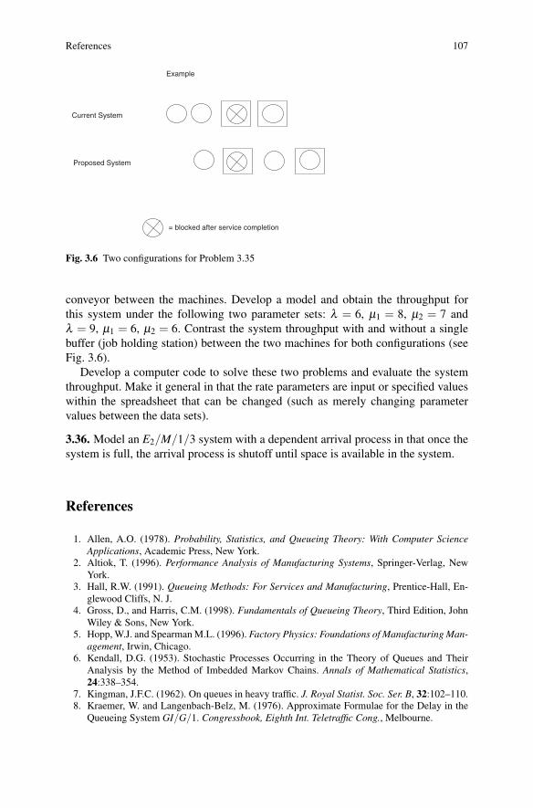
References 107

Current System

Proposed System

Example

= blocked after service completion

Fig. 3.6 Two configurations for Problem 3.35

conveyor between the machines. Develop a model and obtain the throughput forthis system under the following two parameter sets: λ = 6, μ1 = 8, μ2 = 7 andλ = 9, μ1 = 6, μ2 = 6. Contrast the system throughput with and without a singlebuffer (job holding station) between the two machines for both configurations (seeFig. 3.6).

Develop a computer code to solve these two problems and evaluate the systemthroughput. Make it general in that the rate parameters are input or specified valueswithin the spreadsheet that can be changed (such as merely changing parametervalues between the data sets).

3.36. Model an E2/M/1/3 system with a dependent arrival process in that once thesystem is full, the arrival process is shutoff until space is available in the system.

References

1. Allen, A.O. (1978). Probability, Statistics, and Queueing Theory: With Computer ScienceApplications, Academic Press, New York.

2. Altiok, T. (1996). Performance Analysis of Manufacturing Systems, Springer-Verlag, NewYork.

3. Hall, R.W. (1991). Queueing Methods: For Services and Manufacturing, Prentice-Hall, En-glewood Cliffs, N. J.

4. Gross, D., and Harris, C.M. (1998). Fundamentals of Queueing Theory, Third Edition, JohnWiley & Sons, New York.

5. Hopp, W.J. and Spearman M.L. (1996). Factory Physics: Foundations of Manufacturing Man-agement, Irwin, Chicago.

6. Kendall, D.G. (1953). Stochastic Processes Occurring in the Theory of Queues and TheirAnalysis by the Method of Imbedded Markov Chains. Annals of Mathematical Statistics,24:338–354.

7. Kingman, J.F.C. (1962). On queues in heavy traffic. J. Royal Statist. Soc. Ser. B, 32:102–110.8. Kraemer, W. and Langenbach-Belz, M. (1976). Approximate Formulae for the Delay in the

Queueing System GI/G/1. Congressbook, Eighth Int. Teletraffic Cong., Melbourne.


9. Sakasegawa, H. (1977). An Approximation Formula Lq = αβ ρ (1−ρ). Annuals of the Insti-tute of Statistical Mathematics, 29:67–75.

10. Whitt, W. (1983). The Queueing Network Analyzer. The Bell System Technical Journal,62:2779–2814.

http://www.springer.com/978-3-642-16617-4

9783642166174 c1

Technology

steadystate number of

possible system state

nmax1 jobs

expected number of jobs

maximum of nmax jobs

steadystate distribution

busy processing jobs

steadystate probabilities