a comparative study on devs and ns-2 simulation...
TRANSCRIPT

A Comparative Study on DEVS and ns-2 Simulation and Modeling
by
Kahkashan Shaukat
Computer Science & Engineering
School of Computing and Informatics
Arizona State University, Tempe, AZ
&
Hessam Sarjoughian
Arizona Center for Integrative Modeling & Simulation
Computer Science & Engineering
School of Computing and Informatics
Arizona State University, Tempe, AZ
TR-07-006
August 2007

TR-07-006 2
Table of Contents
1 Abstract................................................................................................................................................. 3 2 Introduction........................................................................................................................................... 4
2.1 An example ................................................................................................................................... 5 3 ns-2 Approach....................................................................................................................................... 6
3.1 ns-2 framework ............................................................................................................................. 6 3.1.1 ns-2 class hierarchy .............................................................................................................. 7 3.1.2 Node model .......................................................................................................................... 7 3.1.3 ns-2 scheduling and queuing ................................................................................................ 8 3.1.4 Network animator................................................................................................................. 9
3.2 ns-2 simulation models ................................................................................................................. 9 4 DEVS Approach ................................................................................................................................. 10
4.1 Atomic and coupled model components ..................................................................................... 11 4.2 DEVS simulation models............................................................................................................ 11
4.2.1 Sensor nodes....................................................................................................................... 11 4.2.2 Cluster head........................................................................................................................ 12 4.2.3 Switching unit .................................................................................................................... 13
4.3 The Area model........................................................................................................................... 13 4.4 Experimentation set-up ............................................................................................................... 14
5 Simulation model configuration.......................................................................................................... 15 5.1 Homogeneous and heterogeneous nodes..................................................................................... 15 5.2 Simulation experiments............................................................................................................... 16
6 Conclusions......................................................................................................................................... 19

TR-07-006 3
Abstract
Analysis and design of network systems relies on simulation models that can describe important traits such
as performance and scalability. Essential for specifying network designs are concepts and methods that can
support developing well-formed simulation models. The network simulator ns-2 can be used to model and
simulate high resolution dynamics of network protocols. For developing new or existing application
software systems, the system-theoretic DEVS approach can be used. An illustrative example is developed,
simulated, and analyzed in the ns-2 and DEVSJAVA environments. The example helps to show the kinds
of abstractions afforded by each approach and some key their differences in supporting simulation model
verification and validation.

TR-07-006 4
1 Introduction
Self-organizing networks (i.e., networks that have no centralized infrastructure) are used for software
applications ranging from browsing the Internet, sensor-based managements of resources such as
transportation systems, to snooping on enemy military communications. The increase in distributed systems
based on computer networks has made sensor networks a very active field of research. A particular area of
interest focuses on advanced designs and intricate operation of ad-hoc networks that are energy efficient
and largely independent of the network topology.
Analytical approaches can support describing models of ad-hoc network structures and their
performance under idealized conditions. The models, however, are often limited since it is difficult to
extend them to describe complex network dynamics [7]. The restrictions imposed by analytical approaches
have resulted in increased use of simulation modeling since it is possible to describe and study complexity
inherent in network systems under varying operational conditions [18]. This is because simulation offers a
rich setting for investigating scalable network communication structures and operations [2, 8]. Simulation
modeling affords answering questions (e.g., what are the performance, resource utilization, and flexibility
of networks) that often go unanswered for particular application domains using analytical approaches.
A variety of modeling and simulation approaches exist for studying dynamical systems including
networks [2, 8, 17]. For computer networks, ns-2 [14], GloMoSim [9], and OPNET [16] are used by
researchers and engineers. Within network research community, ns-2 is often used for developing new
protocols whereas for engineering applications, OPNET is used for analysis of existing computer network
system operations and developing new designs. These simulation tools can be broadly viewed to be
developed based on logical processes, queuing theory, and object-orientation programming and design
concepts and techniques. A computer network can be modeled as a network of nodes and links that interact
with one another via input and output messages. The dynamics of the nodes and links are formulated in
terms of discrete-event processes, inputs and outputs that can be executed in alternative sequential or non-
sequential regimes. These models are developed primarily in terms of programming languages that are
formulated in terms of UML and logical processes [4].
Another body of research has focused on modeling of systems including computer networks using the
system concepts and theories. The system concept provides a foundational basis to describe individual
components of a dynamical system in terms of inputs, outputs, states, and transition functions [1, 17]. The
discrete-event formulation of system theory affords modeling sub-systems and their hierarchical
composition as discrete (or continuous) processes with discrete-event (piecewise continuous) inputs and
outputs. The discrete-event and continuous models of a system can be realized in terms of software objects
that can be executed in sequential, parallel, or distributed settings using well-defined abstract simulator
specifications. For example, DEVS realizations such as DEVSJAVA and DEVS-C++ [13] have been used
for modeling computer and social network systems [5, 13, 19]. However, unlike ns-2, there has not been a
concerted effort to create realistic models of network protocols and devices.

TR-07-006 5
It is not uncommon for ns-2, DEVS, and other modeling approaches to be used for purposes that are not
well suited given the strengths and weaknesses of each approach. Furthermore, due to requirements such as
access to source code, cost, government mandate, a modeling approach can have undesirable consequences.
For example, it is important to account for the amount of effort it can take to develop well-formed models
given tradeoffs between (i) conceptualizing and writing models in programming languages, use of open
source software, and availability of detailed model libraries vs. (ii) use of sound model abstractions and
efficient simulation algorithms, ease of model development and simulations, and support for simulation
model verification and validation.
The differences between ns-2 and DEVS modeling approaches has led to synthesizing ns-2 and DEVS-
C++ environments [12]. In particular, DEVS/NS-2 environment has been developed to support modeling a
system in terms of network communication protocols and software application component interactions.
However, it is important to understand the strengths of systems theory as supported by DEVS and the
logical processes as supported by ns-2. In particular, describing a model in ns-2 and DEVS can support
realizing the strengths and weaknesses of these modeling approaches separately as well as the implication
of their integration as in DEVS/NS-2. Such an exposition furthers earlier research on system theoretic and
logical processes as foundational concepts for developing and executing simulation models [15]. It helps to
examine specifying structure and behavior of network systems in terms of well-formed formal model
abstractions instead of programming languages.
In the remainder, we will detail the ns-2 and DEVS model specification capabilities and some challenges
they pose to modelers. We will develop models of a temperature monitoring system for a house in the ns-2
and DEVSJAVA [1] simulation environments. The simulations of the models and the results of these
simulation models are then compared. We conclude with an analysis that underscores the tradeoffs between
developing model abstractions ns-2 and DEVS.
1.1 An example
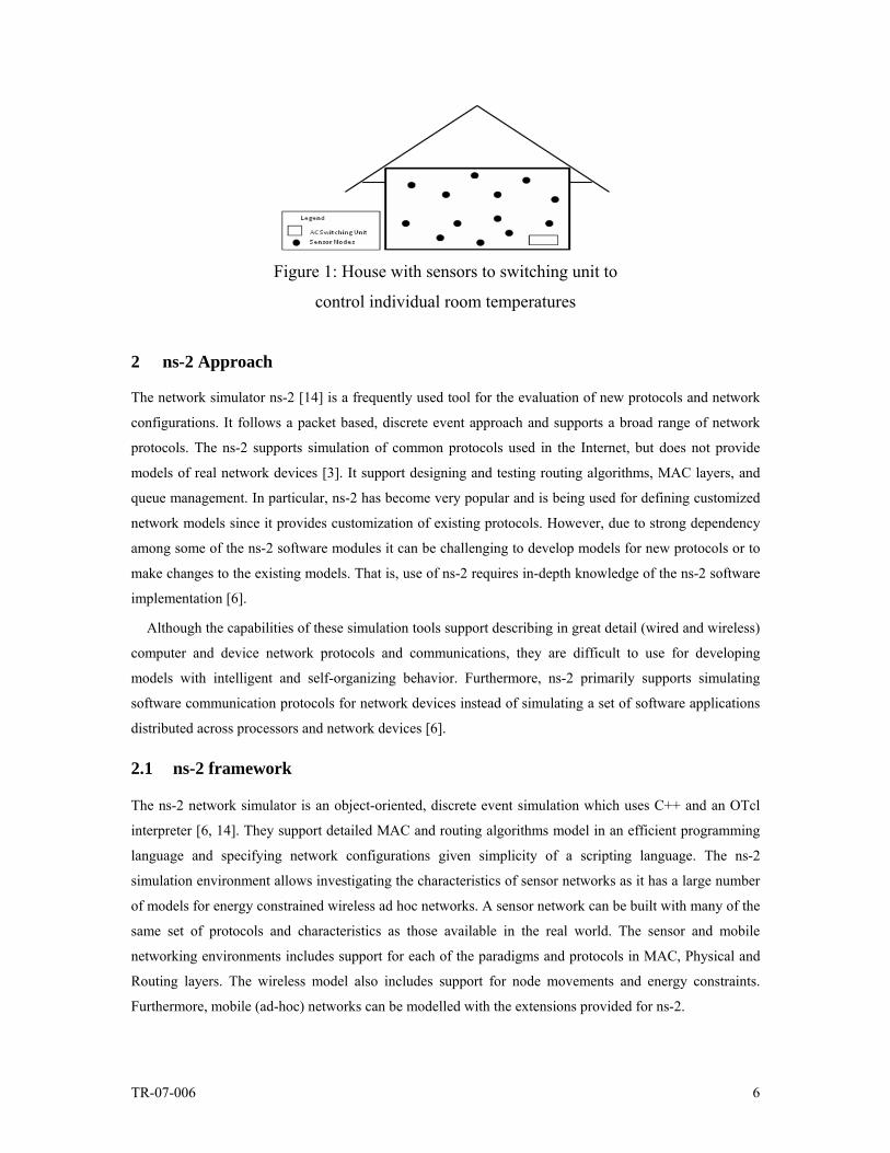
Given a house with several rooms and an air conditioning (AC) unit (see Figure 1), it is useful to determine
where a set of sensors may be placed given that each room’s temperature should be individually controlled.
To achieve a (near) optimal placement of sensors and operation of the AC unit, a house can be modeled as
a set of sensor, AC unit, and rooms. These models of the house will be developed in ns-2 and DEVS
environments and the key aspects of the ns-2 and DEVS approaches will be described.
TR-07-006 6
Figure 1: House with sensors to switching unit to
control individual room temperatures Figure 1
2 ns-2 Approach
The network simulator ns-2 [14] is a frequently used tool for the evaluation of new protocols and network
configurations. It follows a packet based, discrete event approach and supports a broad range of network
protocols. The ns-2 supports simulation of common protocols used in the Internet, but does not provide
models of real network devices [3]. It support designing and testing routing algorithms, MAC layers, and
queue management. In particular, ns-2 has become very popular and is being used for defining customized
network models since it provides customization of existing protocols. However, due to strong dependency
among some of the ns-2 software modules it can be challenging to develop models for new protocols or to
make changes to the existing models. That is, use of ns-2 requires in-depth knowledge of the ns-2 software
implementation [6].
Although the capabilities of these simulation tools support describing in great detail (wired and wireless)
computer and device network protocols and communications, they are difficult to use for developing
models with intelligent and self-organizing behavior. Furthermore, ns-2 primarily supports simulating
software communication protocols for network devices instead of simulating a set of software applications
distributed across processors and network devices [6].
2.1 ns-2 framework
The ns-2 network simulator is an object-oriented, discrete event simulation which uses C++ and an OTcl
interpreter [6, 14]. They support detailed MAC and routing algorithms model in an efficient programming
language and specifying network configurations given simplicity of a scripting language. The ns-2
simulation environment allows investigating the characteristics of sensor networks as it has a large number
of models for energy constrained wireless ad hoc networks. A sensor network can be built with many of the
same set of protocols and characteristics as those available in the real world. The sensor and mobile
networking environments includes support for each of the paradigms and protocols in MAC, Physical and
Routing layers. The wireless model also includes support for node movements and energy constraints.
Furthermore, mobile (ad-hoc) networks can be modelled with the extensions provided for ns-2.

TR-07-006 7
2.1.1 ns-2 class hierarchy
A key appeal for ns-2 is its extensive library of primitive and composite model components. The use of ns-
2 requires expertise in object-oriented programming languages, analysis, and design. This is because
discrete event model abstractions and domain knowledge must be developed conceptualized in terms of the
TclObject class and many others (a simplified subset of the ns-2 classes for the House example is shown in
Figure 2). The TclObject is a superclass of all OTcl library objects scheduler, network components, timers
and the other objects including NAM related ones). The NsObject class is the superclass of all basic
network component objects that handle packets, which may compose compound network objects such as
nodes and links. The basic network components are further divided into Connector and Classifier classes
based on the number of the possible output data paths. The basic network objects that have only one output
data path are under the Connector class, and switching objects that have possible multiple output data paths
are under the Classifier class.
NsO bject
TclO bject
D ropTail R ed Tcp
Classifier
Q ueue D elay Agent
Connector
11 11 11
AddrClassifier
Figure 2: A partial ns-2 class hierarchy
Figure 2
2.1.2 Node model
An abstract view of the basic sensor node model component in ns-2 is depicted in Figure 3. Each sensor
node is an extension of a node that has an address and port classifier. The node is extended to work in
conjunction with the link-layer (LL), the media-access layer (MAC), and the physical layer (PHY)

TR-07-006 8
protocols. In order to support this extension the packet header has been modified. The packet header has a
common header with MAC header, Link Layer header and IP headers added to it (see [6] for details).
addressclas s ifier
radio propagation
C HANNE L
MAC
PHY
L L
IFQ
node entry routing
agent
protocolagent
addressclas s ifier
radio propagation
C HANNE L
MAC
PHY
L L
IFQ
node entry routing
agent
protocolagent
Figure 3: Conceptual SensorNode model adapted
from [12]. Figure 3
2.1.3 ns-2 scheduling and queuing
The ns simulator presently has four available schedulers, each using a different data structure: a simple
linked-list, heap, calendar queue (default), and a special type called “real-time”. The simulator uses seconds
as time units, is single-threaded, and only one event at any given time is executed. If more than one event
are scheduled to execute at the same time, their execution is performed on the first scheduled – first
dispatched manner. Simultaneous events are not reordered anymore by schedulers (as in earlier versions)
and all schedulers should yield the same order of dispatching given the same input. There is no support for
partial execution of events or pre-emption.
ns-2 translates the physical activities of the network to events [14] and maintains a queue of events -
ordered by time a [virtual time]. It repeatedly extracts an event at the queue head, sets [virtual time] =
event’s time, processes and while processing it generates another event, adds it to the queue. Each event
takes predefined amount of virtual time, arbitrary amount of real time, that is, a slow CPU makes
simulation run slower (in real time), but does not change the results.
The queued events are defined by {time, uid, next, handler}, where time is the scheduling time of the
event, uid is the unique id of the event, next is the next scheduled event in the event queue (linked list), and
handler points to the function to handle the event when the event is scheduled. Events are put into the event
queue sorted by their time, and scheduled one by one by the event scheduler. Here, it is important to note
that the class Packet is a subclass of class Event where packets are received and transmitted at some time
with all other network components being subclasses of class Handler which needs to handle events such as
TR-07-006 9
packets. The event at the head of the event queue is delivered to its handler of network object where the
network object may call other network objects, and finally some new events are inserted into the event
queue.
2.1.4 Network animator
In ns-2, generally the nodes in the network are modeled as objects where as the links are just connection
between the nodes. Because the links are not modeled, there is no distinction between multiple links
emerging from the same source but incident on different interfaces of other nodes even though ns-2
provides multiple interfaces. The ns-2 uses Network AniMator (nam) to help user visualize the network
packet transmission, mobility and packet drops.
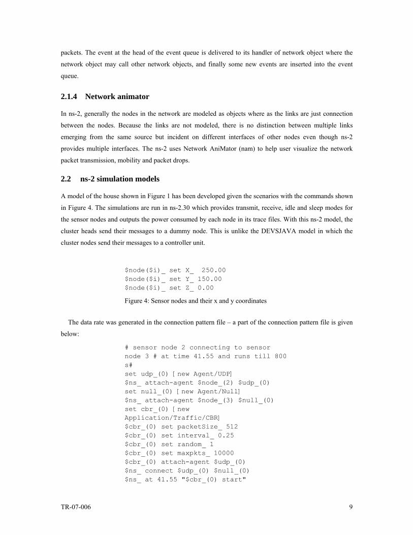
2.2 ns-2 simulation models
A model of the house shown in Figure 1 has been developed given the scenarios with the commands shown
in Figure 4. The simulations are run in ns-2.30 which provides transmit, receive, idle and sleep modes for
the sensor nodes and outputs the power consumed by each node in its trace files. With this ns-2 model, the
cluster heads send their messages to a dummy node. This is unlike the DEVSJAVA model in which the
cluster nodes send their messages to a controller unit.
$node($i)_ set X_ 250.00 $node($i)_ set Y_ 150.00 $node($i)_ set Z_ 0.00
Figure 4: Sensor nodes and their x and y coordinates
Figure 4 The data rate was generated in the connection pattern file – a part of the connection pattern file is given
below:
# sensor node 2 connecting to sensor node 3 # at time 41.55 and runs till 800 s# set udp_(0) [new Agent/UDP] $ns_ attach-agent $node_(2) $udp_(0) set null_(0) [new Agent/Null] $ns_ attach-agent $node_(3) $null_(0) set cbr_(0) [new Application/Traffic/CBR] $cbr_(0) set packetSize_ 512 $cbr_(0) set interval_ 0.25 $cbr_(0) set random_ 1 $cbr_(0) set maxpkts_ 10000 $cbr_(0) attach-agent $udp_(0) $ns_ connect $udp_(0) $null_(0) $ns_ at 41.55 "$cbr_(0) start"

TR-07-006 10
$ns_ at 800.00 "$cbr_(0) stop"
Figure 5: Initialization and data generation rates
Figure 5
The tcl script was appropriately changed to enable the use of different transmission ranges by setting
the different RXTHRESH_ values. We use TwoRayGround Propagation model with RXTHRESH_ values
2.71e-10, 2.81838e-9 and 3.65262e-10 for 90, 150 and 250 m transmission ranges. These values were
calculated using the propagation.cc code under the indep-utils/propagation folder in the ns
folder.
The parameters specific to ns-2 are (i) physical layer: two Ray Ground propagation model, (ii) MAC layer:
802.11, and (iii) Routing: DumbAgent (ideal routing).
# $ns_ node-config # -addressingType flat # -adhocRouting DumbAgent # -llType LL # -macType Mac/802_11 # -propType TwoRayGround # -ifqType Queue/DropTail # -ifqLen 50 # -phyType Phy/WirelessPhy # -antType Antenna/OmniAntenna # -channelType hannel/WirelessChannel# -topoInstance $topo # -energyModel "EnergyModel" # -initialEnergy 700 # -rxPower (in W) # -txPower (in W) # -agentTrace ON # -routerTrace ON # -macTrace ON # -movementTrace ON or OFF
Figure 6: Sensor node configuration
Figure 6 Figure 7
3 DEVS Approach
Discrete EVent System specification (DEVS) is a mathematical modeling formalism for describing
(discrete and continuous) dynamical systems [17]. The generic system-theoretic concepts and mathematical
set theory provide a framework to for specifying models with well-defined structural and behavioral
specifications. This approach lends itself to object-based abstraction, encapsulation, modularity and
hierarchy concepts and implementation. Its simulation protocol enforces causality, concurrency, and timing

TR-07-006 11
among DEVS models. Extension to the DEVS approach supports modeling mobile networks as well as
parallel/distributed execution using classical middleware and service oriented architecture [1].
3.1 Atomic and coupled model components
These components characterize the structure and behavior of individual components with the help of input
(X), output (Y), state (S) sets and functions. The functions internal (δint), external (δext), confluent (δconf),
output (λ) and time advance (ta) define a component’s time-based behavior. The internal and external
transition functions describe autonomous behavior and response to external stimuli, respectively. The
confluent transition function is used to account for cases where the internal and external transition functions
occur concurrently. The time advance function represents passage of time in conjunction with the internal,
external, and confluent transition functions. Output function is used to generate output messages sent
through the output ports of atomic models. Atomic models receive messages which may cause a series of
state transitions and output messages generated for consumption by other atomic or coupled models.
A coupled model specifies the constructs for forming complex models by coupling together multiple
atomic and/or coupled models into hierarchical structures defining a coupled component’s behavior by its
constituent atomic (and/or coupled) models. Because DEVS provide the feature of closure under coupling,
the coupled models themselves can be used as atomic models. Coupled models are constructed
systematically using the concepts of ports and couplings.
Parallel DEVS is capable of processing multiple input events and provides control for handling
simultaneous internal and external events. DEVS atomic and coupled models have computational
counterparts which may be executed in parallel manner using software engineering concepts. DEVSJAVA
is an implementation of the DEVS formalism and its associated simulation protocol [1, 17]. There exist
various implementations of the discrete event system specification approach based on single and
multiprocessor environments. Parallel and distributed environments have been developed using
technologies such as HLA [10].
3.2 DEVS simulation models
The House example shown in Figure 1 is modeled with a set of atomic sensor and cluster heads node
models. Other parts of the House example including rooms, switching unit are modeled as coupled models
described next.
3.2.1 Sensor nodes
These nodes are capable of sensing the temperature and communicating with each other as well as the
cluster heads. The cluster heads, which are also atomic components, have more energy and processing
power than the sensor nodes. Each sensor node is assigned a unique id, name, an (X, Y) coordinate, a
ThHIGH and a ThLOW (ThHIGH = high threshold and ThLOW = low threshold values) and a transmission range.
The nodes are assigned to different cluster heads depending upon the distance between itself and the cluster

TR-07-006 12
head ensuring communication between them. If multiple cluster heads are available, the one which is
closest to the node is assigned as its cluster head. The couplings follow the cluster head assignment. The
sensor nodes sense the current temperature periodically and sends a message to Cluster Heads only when
the observed temperature exceeds a certain threshold value. They also generate messages containing the
current power level of the node; these messages are passed on to the transducer to enable tracking of power
consumption at each node. The cluster heads are responsible for communicating with the outside world –
i.e., they will send the appropriate messages to the Switching Unit SWITCH ON or TURN OFF the cooling
system.
3.2.2 Cluster head
The Cluster Head model is similar to the Sensor Node Model except that it processes messages from the
sensor nodes and generates the next message that it has to send to the Switching Unit. It can also have the
capability to sense the temperature of the room. A component view of the Cluster Head showing model
name, input and output ports and state equals to sensing is shown in Figure 7. A formal specification of the
Cluster Head is given in Figure 8.
Figure7: cluster head atomic model component
Figure 7 ClusterHeadprocessing_time = <XM,YM,SM,δext,δint,δconf,ta,λ> Iports = {“in”,“inSN”,“stop”}, where XinSN є {Input_messages} and Xstop = an
entity Input_messages = {( node_id, ThHIGH, ThLOW, key, time) | node_id є Node_ID,
key є {cool, heat}} and time is a function of the difference of the current temperature and one of the two threshold values depending on the key}and Node_ID = { i, 0 < i < N | i є of the members of the same cluster}
XM = {(p,v) | p є IPorts, v є Xp} is the set of input ports and values; Oports = {“out”,“queryOut”,“toTransd”} YM = {(p,v) | p є OPorts, v є Yp} is the set of output ports and values; where
Yout є Output_messages} and YtoTransd є {(node_name, power_level)} here node_name = {ClHead0, ClHead1, …, ClHeadn}
Output_messages = {( node_id,ThHIGH,ThLOW,key,time1) | node_id є Node_ID, key є
{cool, heat}} and time1 = time –1 if time > 0 or time1 = time } and Node_ID = { i, 0 < i < N | i є of the members of the same cluster}
S = {sensing,sleeping,send_msg,dead,passive} × R0+ × Xp

TR-07-006 13
δext ((phase,σ,prev_temp,Q), e,((“inSN”, x1), (“inSN”,x2), …, (“inSN”,xn))) = (send_msg, 0, prev_temp, Q/) if phase is “sensing”, x1, x2, …, xn є
Xin; for each xi, 0 < i < n, prev_temp[i] = xi.curr_temp and |Q/| = |Q| + n = (send_msg,σ – e,prev_temp,Q/) otherwise, prev_temp = prev_temp and
|Q/| = |Q| δext ((phase,σ,prev_temp),e,(“stop”, x)) = (passive,∞,prev_time,Q) prev_temp = prev_temp and |Q/| = |Q| δint (phase,σ,prev_temp,Q) = (dead,∞,prev_temp,Q) if phase is “send_msg”, power < min_power,
prev_temp = prev_temp and |Q/| = |Q| = (sleeping,∞,prev_temp, Q) if phase is “send_msg”, power > min_power,
prev_temp = prev_temp and |Q/| = |Q| = (dead, ∞, prev_temp, if phase is “sleeping”, power < min_power,
prev_temp = prev_temp and |Q/| = |Q = (sleeping,∞,prev_temp,Q) if phase is “sleeping”, power > min_power,
prev_temp = prev_temp and |Q/| = |Q| λ (phase,σ,prev_temp,Q) = Yout if phase = send_msg, power> min_power, while
|Q| ≠ 0 λ (phase,σ,prev_temp,Q) = YtoTransd if phase = send_msg, power> min_power,
while |Q| ≠ 0
ta(phase,σ,prev_temp,Q) = σ
Figure 8: Atomic model specification of a node
Figure 8
3.2.3 Switching unit
The Switching Unit consists of the Controller Unit and the Heat/Cool Unit. The Controller Unit gets the
message sent by the cluster heads which sends Control Messages to the Heat/Cool Unit.
The Heat/Cool unit processes each of the messages sent by the Controller unit and generates a
temperature for each of the nodes sending On/Off Messages to the cluster heads. If a node’s message holds
the key to cool, the Heat/Cool Unit will generate a temperature which is less than the temperature that it
generated in the previous iteration. Otherwise, the temperature generated is greater than the previous
temperature. These messages are sent to each of the sensor nodes and the process continues until the end of
simulation time is reached or the sensor nodes or the cluster heads die out due to power consumption.
3.3 The Area model
The Area model is a coupled model consisting of one or more Room models and a corresponding
Switching Unit for the Room model (see Figure 11). The Room model consists of a number of Sensor Node
and Cluster Head models. The cluster head then processes the On/Off Request message and extracts the
time parameter from the message. This is the period of time for which the sensor node will go to sleep. The
cluster head then sends the information of each member of its cluster to the Switching Unit. For the

TR-07-006 14
experiment purposes, only one room has been implemented. It can very easily be increased to multiple
rooms.
The Room models are identical except that they refer to the partitioning between different rooms that can
have different thresholds. The area to be monitored can be partitioned into any number of rooms which
implies the duplication of these components, their ports and couplings. Each room consists of a number of
sensor nodes, some of which are designated as cluster heads. The cluster heads are similar to any other
sensor node except that they are connected to the controller and can communicate with it directly or
indirectly through other cluster heads. The cluster heads can also sense the temperature. They also have the
capability to query the sensor nodes in their vicinity about the temperature at point of time.
Figure 9: The Temperature monitoring system modeled using DEVSJAVA Figure 9
3.4 Experimentation set-up
To systematically experiment with the Area model, an Experimental Frame model is devised. It consists
two Transducers (refer to Figure 9). One keeps track of power consumed by the sensor nodes and the other
tracks the period of time the Heat/Cool Unit remains on or off. The cluster heads then can communicate
with the Controller unit and send the appropriate request.
If there is only one cluster head in a segment, the network topology is a STAR topology, the simplest to
solve. Only this cluster head is connected to the Controller unit. In the first scenario, only one-hop transfer
of information is required. In the second scenario, there are multiple cluster heads in any room and all the
cluster heads are able to communicate with the Controller. This forms a network, but the message can be
reached from the sensor node to the controller in two-hops as the STAR topology.

TR-07-006 15
The experimental frame supports conducting different experiments with the model – e.g., changing the
transmission range, the threshold levels, homogeneous and heterogeneous environments. The experimental
frame observes average power consumption of the nodes and calculates the average life of a node.
Furthermore, it can be used to define time- or state-based conditions under which the simulation can be
terminated.
4 Simulation model configuration
Simulations were both in DEVSJAVA and ns-2, the common parameters for both the simulations are
provided below in Table 1.
Table 1: Common simulation parameters
Two different models have been implemented in DEVSJAVA version 2.7 where MODEL1 has the
capability to handle different threshold values for each of the sensor nodes. This is similar to the case where
many people sitting in the same room can have different settings for the temperature with the temperature
being monitored accordingly. MODEL2 is a simplified version which has the same threshold values for all
the sensor nodes in one particular room. The same models have been used in the ns-2 simulations. The
different scenarios are described below:
4.1 Homogeneous and heterogeneous nodes
The sensor nodes (SN) and the cluster heads (CH) can have identical or different levels of power. For
example, if we consider homogeneous sensor nodes, the sensor nodes and the cluster heads are assigned the
same level of power. For example, they are assigned 700 units. For heterogeneous nodes, the power level of
SNs is set to 700 units and that of the CHs is set to 1000 units.
i) The number of sensor nodes: can be changed but this has very little effect in power consumption
or average life of a node.
Parameters Values
Time 800 s Sensor Node 10 (can be changed but has little effect on power
consumption of the sensors) Cluster Head 4 (observed during experimentation that cluster heads
need to be at least 30% of the sensors) Initial Power 700, 1000 J No of runs 3 Transmission
Range [250, 150, 90] m
THHIGH 78 – 80 degrees Fahrenheit THLOW 68 – 70 degrees Fahrenheit Area 500 m by 500 m

TR-07-006 16
ii) Cluster Heads: observed during the simulations that the number of cluster heads in a room need to
be at least 30% of the number of sensor nodes, otherwise, some sensor nodes are unable to form
clusters.
iii) MODEL1: sensor nodes each having different threshold values.
iv) MODEL2: all sensor nodes having the same threshold values.
The statistics files generated by the Transducers are shown in Tables 2, 3 and 4 with the transmission
range of 250m, 150m and 90m respectively. Here, Power Consumption = EC, Average Sensor Life =
Av(SNL), Cluster Head Life = CHL, mODEL1 = M1 and MODEL2 = M2.
4.2 Simulation experiments
The ns-2 and DEVSJAVA simulation results for the scenarios described above are shown in Figures 10
through 15. The simulation plots show that the ns-2 and DEVS models have similar behavior.
Figure 10: Energy consumption for MODEL1 and
MODEL2 with transmission range of 250 m. Figure 10
We see that with 250 m transmission range, the energy consumption is the highest while the network life
is the lowest – this is as expected; more energy drainage occurs at the sensor nodes and cluster heads as
their transmission range increases (they have increased number of neighbors that each can listen to). The
ns-2 homogeneous model shows that the sensor nodes and the cluster heads all consume the same amount
of energy
TR-07-006 17
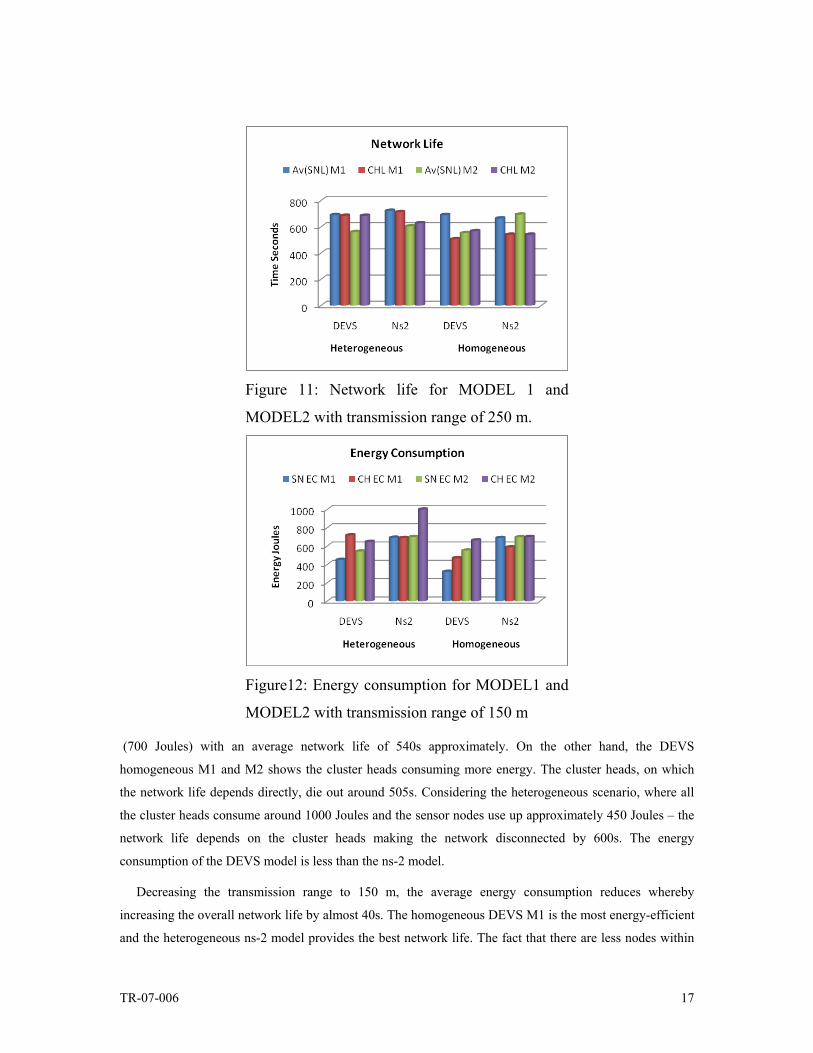
Figure 11 Figure 12
Figure 11: Network life for MODEL 1 and
MODEL2 with transmission range of 250 m.
Figure12: Energy consumption for MODEL1 and
MODEL2 with transmission range of 150 m
(700 Joules) with an average network life of 540s approximately. On the other hand, the DEVS
homogeneous M1 and M2 shows the cluster heads consuming more energy. The cluster heads, on which
the network life depends directly, die out around 505s. Considering the heterogeneous scenario, where all
the cluster heads consume around 1000 Joules and the sensor nodes use up approximately 450 Joules – the
network life depends on the cluster heads making the network disconnected by 600s. The energy
consumption of the DEVS model is less than the ns-2 model.
Decreasing the transmission range to 150 m, the average energy consumption reduces whereby
increasing the overall network life by almost 40s. The homogeneous DEVS M1 is the most energy-efficient
and the heterogeneous ns-2 model provides the best network life. The fact that there are less nodes within

TR-07-006 18
the communication range lowers down the energy consumption as less number of nodes interfere with each
other. The heterogeneous DEVS M1 provides a better network life of around 715s. None of the models
survive the whole simulation time (800s) – the cluster heads in the heterogeneous DEVS M1 consume
more energy compared to the heterogeneous DEVS M2, and the homogeneous models contributed by the
fact that sensors have different threshold values for heterogeneous M1, by possibly increased the sensor
activity and reduced sleep time. The same logic is valid for the cluster heads which have to transmit more
messages in order to keep the temperature controlled.
Figure13: Network life for MODEL1 and MODEL2 with
transmission range of 150 m
Figure 13 Further reducing the transmission range of the sensors, we see that all the models and their variations
increase the life of the network so that all the models are able to run to the end of the simulation period. In
case of the heterogeneous models, the cluster heads consume almost all of their energy but because the
range for communication is lower, the network life is enhanced.
Figure14: Energy consumption for MODEL1 and

TR-07-006 19
MODEL2 with transmission range of 90 m
Figure 14
Figure15: Network life for MODEL1 and MODEL2 with
transmission range of 90 m
The results show us that both the DEVS and the ns-2 models perform similarly when the transmission
range is reduced – that is, in each case the network life is increased and the cluster heads do not die out as
soon as when the transmission range was larger. The same trend can be seen when we use sensors with
different temperature thresholds, the sensors and the cluster heads all consumed more energy due to the
increased sensor activity and reduce the network life. Thus, we can see that both the simulators produce
similar results and are thus useful for simulating networks.
Figure 15
Homogeneous M2 consumes the least amount of power and all the sensor nodes and the clusters heads
remain alive at the end of the simulation time. This is the most simplistic scenario and the results show the
behavior to be the simplest for this model.
5 Conclusions
It has been shown that although ns-2 and DEVS modeling approaches can be used to model and simulate
network systems, the modelers must have different skill sets. Using the DEVS approach, modelers use
system concepts with formal constructs to specify structure and behavior of models. Rather than developing
models in terms of Java and C++ programming constructs, network models can be specified and
systematically and semi-automatically mapped to simulation models. These models can be executed in
DEVS simulation environments implemented in Java or C++. In contrast, in ns-2, models need to be
developed in terms of Otcl and C++ programming constructs. Modelers may use UML to develop
abstractions. While UML offers higher level abstraction to conceptualize and specify models, it is not
suitable for specifying simulation models [7]. Other key considerations are choosing a modeling and

TR-07-006 20
simulation approach is its support for verification and validation and the availability of rich network
protocols model libraries that have community wide acceptance. Given these considerations for the DEVS
and ns-2 approaches, further research can be undertaken to increase rigor in model development while
reducing efforts in model development and simulation studies. Other key benefits are stronger support for
verification and validation, visual model development, and semi-automatic simulation code generation.
Such capabilities can significantly simplify model development, reduce cost, and help improve confidence
in simulation models and results produced from them.

TR-07-006 21
References
[1] ACIMS. Arizona Center for Integrative Modeling and Simulation, 2001,
http://www.acims.arizona.edu/SOFTWARE.
[2] Banks, J., Carson, J., Nelson, B.L., and Nicol, D., Discrete-Event System Simulation, 4th ed, 2004:
Prentice Hall, 624.
[3] Baumgartner, F., Scheidegger, M., and Braun, T. Enhancing discrete event network simulators with
analytical network cloud models, International Workshop Inter-domain Performance and Simulation,
2003, p. 21-30, Salzburg.
[4] Chandy, K.M. and Misra, J., Asynchronous Distributed Simulation via a Sequence of Parallel
Computations, Communications of the ACM, 1981, 24(11): p. 198-205.
[5] Cho, T.H. and Kim, H.J., DEVS Simulation of distributed intrusion detection systems, Transactions of
the Society for Computer Simulation International, 2001, 18(3): p. 133-146.
[6] Fall, K. and Varadhan, K. The ns manual, 2005, http://www.isi.edu/nsnam/ ns/doc/ns_doc.pdf.
[7] Floyd, S. and Paxson, V., Difficulties in Simulating the Internet, IEEE/ACM Transactions on
Networking, 2001.
[8] Fujimoto, R.M., Parallel and Distributed Simulation Systems, 2000: John Wiley and Sons, Inc.,
xvii+300.
[9] GloMoSim. GloMoSim Simulation Layers, 2004, http://pcl.cs.ucla.edu/projects/glomosim/.
[10] Hall, S., DEVS/HLA MEASURE Testbed, 2000, Lockheed Martin Corporations: Personal
Communication.
[11] Huang, D. and Sarjoughian, H. Software and Simulation Modeling for Real-Time Software-Intensive
Systems, 8th IEEE International Symposium on Distributed Simulation and Real-time Applications,
2004, p. 196-203, Montreal, Canada.
[12] Kim, T., Huang, M.H., Kim, D., and Zeigler, B., DEVS/NS-2 Environment: Integrated Tool for
Efficient Networks Modeling and Simulation, DEVS Symposium, Spring Simulation Conference,
2007. p. Norfolk, VA.
[13] Kim, Y.J., Kim, J.H., and Kim, T.G., Heterogeneous Simulation Framework Using DEVS BUS,
Simulation, 2003, 79(1): p. 3-18.
[14] ns-2. Network Simulator, 2002, http://www.isi.edu/nsnam/ns/.
[15] Nutaro, J.J. and Sarjoughian, H.S., Design of Distributed Simulation Environments: A Unified System-
Theoretic and Logical Processes Approach, Simulation, 2004, 80(11): p. 577-589.
[16] OPNET. OPNET Modeler, 2005, http://opnet.com.
[17] Zeigler, B.P., Praehofer, H., and Kim, T.G., Theory of Modeling and Simulation: Integrating Discrete
Event and Continuous Complex Dynamic Systems, Second Edition, 2000: Academic Press.

TR-07-006 22
[18] Zeigler, B.P., Sarjoughian, H.S., and Ghosh, S. Workshop on Modeling and Simulation of Ultra-Large
Networks: Challenges and New Research Directions, 2001,
http://www.acims.arizona.edu/EVENTS/ULN01/ULN01MainPage.htm.
[19] Zengin, A. and Sarjoughian, H.S. Honeybee Inspired Discrete Event Network Modeling: Approach
and Experimentation, 16th European Simulation Symposium, 2004. p. 317-324, Oct., Budapest,
Hungary.