a comparison of breeding and ensemble transform...

1140 VOLUME 60J O U R N A L O F T H E A T M O S P H E R I C S C I E N C E S

q 2003 American Meteorological Society

A Comparison of Breeding and Ensemble Transform Kalman Filter EnsembleForecast Schemes

XUGUANG WANG

The Pennsylvania State University, University Park, Pennsylvania

CRAIG H. BISHOP

UCAR, Boulder, Colorado, and Naval Research Laboratory, Monterey, California

(Manuscript received 28 May 2002, in final form 1 November 2002)

ABSTRACT

The ensemble transform Kalman filter (ETKF) ensemble forecast scheme is introduced and compared withboth a simple and a masked breeding scheme. Instead of directly multiplying each forecast perturbation with aconstant or regional rescaling factor as in the simple form of breeding and the masked breeding schemes, theETKF transforms forecast perturbations into analysis perturbations by multiplying by a transformation matrix.This matrix is chosen to ensure that the ensemble-based analysis error covariance matrix would be equal to thetrue analysis error covariance if the covariance matrix of the raw forecast perturbations were equal to the trueforecast error covariance matrix and the data assimilation scheme were optimal. For small ensembles (;100),the computational expense of the ETKF ensemble generation is only slightly greater than that of the maskedbreeding scheme.

Version 3 of the Community Climate Model (CCM3) developed at National Center for Atmospheric Research(NCAR) is used to test and compare these ensemble generation schemes. The NCEP–NCAR reanalysis data forthe boreal summer in 2000 are used for the initialization of the control forecast and the verifications of theensemble forecasts. The ETKF and masked breeding ensemble variances at the analysis time show reasonablecorrespondences between variance and observational density. Examination of eigenvalue spectra of ensemblecovariance matrices demonstrates that while the ETKF maintains comparable amounts of variance in all or-thogonal and uncorrelated directions spanning its ensemble perturbation subspace, both breeding techniquesmaintain variance in few directions. The growth of the linear combination of ensemble perturbations that max-imizes energy growth is computed for each of the ensemble subspaces. The ETKF maximal amplification isfound to significantly exceed that of the breeding techniques. The ETKF ensemble mean has lower root-mean-square errors than the mean of the breeding ensemble. New methods to measure the precision of the ensemble-estimated forecast error variance are presented. All of the methods indicate that the ETKF estimates of forecasterror variance are considerably more accurate than those of the breeding techniques.

1. Introduction

Since ensemble forecasting was recognized as a prac-tical way for providing probabilistic forecasts in theearly 1970s (Leith 1974), ensemble generation schemeshave been developed and used in weather predictioncenters, for example, the breeding method (Toth andKalnay 1993, 1997) used at the U.S. National Centersfor Environmental Prediction (NCEP), the singular vec-tor method (Buizza and Palmer 1995; Molteni et al.1996) applied at the European Centre for Medium-Range Weather Forecasts (ECMWF), and the systemsimulation method (Houtekamer et al. 1996) used at theCanadian Meteorological Centre (CMC).

Corresponding author address: Xuguang Wang, Department ofMeteorology, The Pennsylvania State University, 503 Walker Build-ing, University Park, PA 16802.E-mail: [email protected]

Previous comparisons of the skills of these ensemblegeneration schemes include that of Houtekamer and De-rome (1995) who found that although these three en-semble generation schemes are fundamentally different,their medium-range ensemble mean error reductionskills are quite comparable given that all initial pertur-bations are centered around the control analysis. Hamillet al. (2000) further studied the ensemble spread skillof these three ensemble generation schemes. They foundthat the singular vector and breeding methods produceless skillful probabilistic forecasts than a variant of thesystem simulation method known as the perturbed ob-servation method.1 This is partly due to a strongerspread–skill relationship in the perturbed observationensemble.

1 In the system simulation method uncertainties in both model phys-ics and the initial condition error are accounted for.

1 MAY 2003 1141W A N G A N D B I S H O P

Compared to a single control forecast, an ensembleforecast not only provides a more accurate estimate ofthe first moment (the mean) of the probability densityfunction (PDF) of future atmospheric states, but alsoprovides higher-order moment estimations such as theforecast error variance. Studies by Toth et al. (2001)argued that the major extra information provided byensemble forecasts relative to a single control forecastis that ensemble forecasts can estimate the case to casevariations in forecast uncertainty. Zhu et al. (2002) alsoattributes much of the economic value of an ensembleforecast to its ability to forecast regional and temporalvariations in forecast error variance. Thus, measuringerror variance prediction accuracy is an important cri-terion in evaluating an ensemble forecast system.

The basic idea behind an ensemble generation schemeis to generate independently perturbed initial conditionssuch that the covariance of the ensemble perturbationsapproximates the analysis error covariance matrix at theinitial time and thus the forecast error covariance matrixat the forecast time. For an optimal data assimilationscheme, the analysis error covariance matrix Pa and theforecast error covariance Pf are related by

21a f f T f T fP 5 P 2 P H (HP H 1 R) HP , (1)

where the matrix H is the linear observation operatorthat maps model variables to observed variables and thematrix R is the observation error covariance matrix. Thenotational convention in this paper is roughly consistentwith Ide et al. (1997). There are two major character-istics in Eq. (1). First, the error variance reduction varieswith geographical variations of observation density andaccuracy. Second, error variance in directions with largeforecast error variance is reduced by a larger factor thanerror variance in directions with small forecast errorvariance is reduced (see appendix and/or Daley 1991);in other words, data assimilation schemes use obser-vations to filter out the most uncertain or ‘‘noisy’’ as-pects of the forecast first-guess field. To provide ac-curate estimate of Pa and Pf , an ensemble generationscheme should be able to reflect these two character-istics.

Of all ensemble generation schemes, the breedingmethod is the most computationally inexpensive. A hy-pothesis of the breeding method is that the importantpart of analysis errors is the dynamically constrainedpart contributed by errors of the forecast background.In the simple form of the breeding method (Toth andKalnay 1993), forecast perturbations are transformedinto analysis perturbations by multiplying a globallyconstant factor whose magnitude is less than one so thatthe size of the scaled forecast perturbations is consistentwith the empirically estimated global analysis uncer-tainty. Consequently, perturbation amplitude does notreflect geographical variations in the observational net-work density and accuracy nor does it reflect the factthat data assimilation schemes reduce error variance indirections corresponding to large error variance by a

larger factor than error variance in directions corre-sponding to small error variance. To allow bred-pertur-bation amplitude to reflect geographical variations inthe observational network, Toth and Kalnay (1997) in-troduced a regional rescaling method where perturba-tions at all levels are multiplied with a geographicallydependent rescaling factor. We shall refer to this moresophisticated breeding scheme as ‘‘masked breeding.’’While masking enables perturbation amplitude to reflectgeographical variations in observational density and ac-curacy, it has a severely limited ability to make pertur-bation amplitudes reflect the fact that data assimilationschemes attenuate error variance in directions corre-sponding to large forecast error variance more than indirections corresponding to small forecast error vari-ance.

The ensemble transform Kalman filter (ETKF) theorywas first introduced as an adaptive sampling method(Bishop et al. 2001). It produces initial perturbationsconsistent with the error covariance update equation (1)within the vector subspace of ensemble perturbations.Thus, one would expect the aforementioned two prob-lems from the breeding scheme would be ameliorated(see section 2c in detail). Different from other ensemble-based Kalman filter (EnKF) theories that have been ex-plored for data assimilation (Houtekamer and Mitchell1998, 2001; Hamill and Snyder 2000; Hamill et al. 2001;Whitaker and Hamill 2002; Anderson 2001), the ETKFensemble is used to estimate Pf only for predicting Pa,not for updating the mean state. Thus, the control anal-ysis used in the ETKF is potentially not as accurate asthe control analysis created in the EnKF data assimi-lation schemes. However, the computational expense ofthe ETKF ensemble generation is considerably less thanthe EnKF ensemble.

To gain insight into the differences between the breed-ing and ETKF ensemble generation schemes, it is help-ful to first consider the types of perturbations eachscheme would produce in an idealized system for a time-invariant linear dynamics, fixed observational network,fixed observation error statistics, and no model error. Insuch an system, forecast covariances at time tk is relatedto analysis covariances at time tk21 by

f a TP 5 MP M ,k k21 (2)

where M is the linear dynamics operator. According toCohn and Dee (1988), in such a system the Kalmanfilter asymptotically approaches a steady state when thesystem is observable. Closed form solutions for the ex-act error covariances that would be produced by infinitetime Kalman filter scheme for such a system are givenin Bishop et al. (2003, hereafter BRT). It demonstratesthat all nondecaying eigenvectors (or normal modes) ofM are required to precisely describe the forecast andanalysis error covariances in such a system with Kalmanfilter for an infinite time. With a fixed dynamics prop-agator, the simple breeding method is equivalent to thepower method for finding the eigenvector corresponding


to the largest eigenvalue of M. Consequently, pertur-bations produced by the simple breeding method wouldall eventually point in the direction of the leading ei-genvector (or normal mode) of M. Thus, for the simplebreeding ensemble, the rank of the ensemble-based sam-ple covariance matrix would be limited to 1.2 From Cohnand Dee (1988) and BRT, in such an idealized system,error covariances started from any initial (at t0) estimate,updated by Eq. (1), and propagated by Eq. (2), willeventually (at t`) converge toward the error covariancesfor an infinite time optimal scheme if the initial estimatecovers all amplifying normal modes that the true initialanalysis/forecast error covariance would cover. Sincethe ETKF perturbations satisfy (1) and (2) in such anidealized system, they would eventually (at t`) providea precise description of the forecast and analysis errorcovariances that an infinite time optimal data assimi-lation scheme would have if the ETKF initial ensembleperturbations span the vector space of unstable normalmodes of the dynamics operator.3 Thus, the ETKF en-semble would be expected to markedly outperform thebreeding ensembles in estimating the forecast/analysiserror covariances in such an idealized system. A com-parison of the performance of the ETKF, the simplebreeding, and the masked breeding ensembles in an im-perfect system where the dynamics propagator is im-perfect and time-dependent and the number of ensemblemembers is less than the number of growing normalmodes of the dynamics operator is the primary aim ofthis paper.

A description of the ETKF and breeding ensemblegeneration schemes is given in section 2. Section 3 pro-vides a brief introduction of the model, the analysis data,the observational network, and the specific construc-tions of initial perturbations. Section 4 compares initialperturbations in terms of effective rescaling factors. Sec-tion 5 compares the dimension of the subspaces in whichensemble variance is maintained. Section 6 comparesthe maximal growth within ensemble perturbation sub-spaces under the total energy norm. Section 7 comparesthe ensemble forecast skills in terms of ensemble mean.In section 8, we introduce methods to measure the errorvariance prediction accuracy and perform comparisonsbetween the ETKF and breeding schemes. The com-putational expense of the techniques is compared in sec-tion 9. Section 10 summarizes our results.

2. Ensemble generation methodsa. Simple breeding

Following Toth and Kalnay (1993), a global constantfactor is applied to each raw forecast perturbation so

2 In cases where there were n . 1 eigenvectors corresponding tothe same largest eigenvalue, the rank would be limited by n.

3 In case not all amplifying normal modes of the linear dynamicsoperator have errors initially, the statement is true when the ETKFinitial perturbations exclude these error-free amplifying normalmodes.

that the scaled perturbation has the same size as theempirically determined global analysis root-mean-square (rms) error. Mathematically,

a fx 5 x · c, (3)

where vectors xa and xf represent an analysis pertur-bation and a forecast perturbation. Scalar c is a constantglobally for each raw perturbation. In our experiment,the value of c for each forecast perturbation is chosenso that 12-h ensemble forecast variance is consistentwith the 12-h control forecast error variance on a glob-ally averaged basis. Details of the method for doing thisare given in section 2c and section 3d.

b. Masked breeding

The global constant factor c in Eq. (3) cannot reflectthe geographically dependent analysis uncertainty. Themasked breeding (Toth and Kalnay 1997) amelioratesthis problem with a regional rescaling factor. Mathe-matically,

a fx 5 x c ,ij ij ij (4)

where and are elements in xa and xf at latitude ia fx xij ij

and longitude j. The mask is a function of latitude andlongitude whose values bound the vertically averagedand horizontally smoothed ensemble perturbation am-plitude. The amplitude for each ensemble perturbationis measured under a user-specified norm that, in ourexperiment, is the square root of vertically averagedsquared wind perturbations. Denote the mask as eij andthe vertically averaged and horizontally smoothed fore-cast perturbation amplitude as . The rescaling factorfyij

is determined for each forecast perturbation as

f 1 y # eij i jc 5 (5)i j eij f y . e .i j i jfy i j

The rescaling factor cij is only a function of latitude andlongitude. It applies to all variables at all levels. In ourexperiments, an inflation factor is applied after (5) inorder to ensure that 12-h ensemble forecast variance isconsistent with the 12-h control forecast error varianceon a globally averaged basis (again, see below for de-tails).

c. ETKF

The ensemble transform Kalman filter is a suboptimalKalman filter (Kalman 1960; Kalman and Bucy 1961;Daley 1991) with the forecast error covariance matrixestimated by the covariance matrix of the ensemble fore-cast perturbations. As mentioned in the introduction,compared to other ensemble-based Kalman filters, thePf estimated by the ETKF is not for updating the meanstate but only for estimating Pa.

Different from the breeding method that transforms


forecast perturbations into analysis perturbations bymultiplying each forecast perturbation by a constant orregional rescaling factor, the ETKF method transformsforecast perturbations into analysis perturbations by atransformation matrix T, that is,

a fX 5 X T, (6)

where forecast perturbations are listed as columns in thematrix Xf and analysis perturbations are listed as col-umns in the matrix Xa. In our experiment, since we useone-sided perturbations, ensemble mean at the initialtime is degraded compared to the control analysis. Soin our one-sided ensemble system, we define analysisand forecast perturbations as deviations from the con-trol, that is, Xa 5 ( 2 , 2 , . . . , 2 ) anda a a a a ax x x x x x2 1 3 1 K 1

Xf 5 ( 2 , 2 , . . . , 2 ), where subscriptf f f f f fx x x x x x2 1 3 1 K 1

1 denotes the control and K is the number of ensemblemembers including the control. The transformation ma-trix T is chosen to solve Eq. (1) provided that

Tf f fP 5 Z (Z ) and (7)a Tf T fP 5 Z TT (Z ) , (8)

where Zf 5 Xf / . Thus, if the covariance matrixÏK 2 1of the raw forecast perturbations Xf were equal to thetrue forecast error covariance matrix Pf , and the dataassimilation scheme were optimal, then the covariancematrix associated with the transformed perturbations Xa

would be precisely equal to the true analysis error co-variance matrix.

Following Bishop et al. (2001), T is given by

21/2T 5 C(G 1 I) , (9)

where columns of the matrix C contain the eigenvectorsof (Zf )THTR21HZf , and the nonzero elements of the di-agonal matrix G contain the corresponding eigenvalues;that is,

T 21f T f T(Z ) H R HZ 5 CGC . (10)

Since (Zf )THTR21HZf is a real symmetric matrix, its ei-genvalues are real and its eigenvectors are orthogonal.Note that the solution to (8) is nonunique. If Bi is a (K2 1) 3 (K 2 1) matrix and Bi 5 I, then substitutionTBi

of Ti 5 TBi in place of T in (8) shows that Ti is also asolution to (8). Differing Bi correspond to the differingdeterministic square root filters discussed in Tippett etal. (2003), of which the ETKF is but a single example.A distinguishing feature of analysis perturbations pro-duced by the ETKF is that they are orthogonal in nor-malized observation space. To see this, premultiply andpostmultiply (10) by T T and T, respectively, and sub-stitute T on the right-hand side by (9). Then we obtain

T 21 21T f T fT (Z ) H R HZ T 5 G(G 1 I) . (11)

The right-hand side of (11) is a diagonal matrix. Thus,from the definition of the ETKF analysis perturbationsin (6), the ETKF analysis perturbations are orthogonalunder the inner product defined by

21T{w; z} 5 wH R Hz, (12)

where w and z are any two vectors with the length ofa state vector. In other words, the analysis perturbationsover the observation sites normalized by the square rootof the observation error covariance matrix are orthog-onal under a Euclidean norm. Note that after normali-zation each element of the analysis perturbations overthe observation sites is dimensionless.

Because the ETKF rotates and rescales perturbationsaccording to the optimal data assimilation equation (1),it is the distribution and quality of observations thatcontrols perturbation amplitude. Furthermore, consis-tent with the filtering properties of an optimal data as-similation scheme, ensemble variance in directions cor-responding to large ensemble variance is reduced by alarger factor than ensemble variance in directions cor-responding to small ensemble variance is reduced (seeappendix and/or Daley 1991). Consequently, one wouldexpect the aforementioned problems of the breedingmethods to be ameliorated by the ETKF method. Ac-cording to the discussion in the introduction about errorvariance characteristics of the ETKF and breedingschemes in an idealized system, one would also expectthat the ETKF ensemble perturbations to maintain var-iance in a much wider range of amplifying directionsthan the breeding ensemble perturbations.

When the number of ensemble perturbations is muchsmaller than the number of directions to which the fore-cast error variance projects, (8) significantly underes-timates total analysis error variance because it lackscontributions from important parts of the error space.To ameliorate this problem, we multiply the transformedperturbations by an inflation factor so as to ensure thatthe global 12-h forecast ensemble variance is consistentwith the global control forecast error variance at therawinsonde sites. Denote ti as the perturbation initiali-zation time. In our experiment, the time interval betweenti and ti11 is 12 h. We hope to find a scalar inflationfactor P i at time ti and multiply the transformed per-turbation obtained at ti by Pi, that is,

a fX 5 X T P ,i i i i (13)

so that we could expect for the next 12-h forecast, name-ly, at time ti11,

T e T˜ ˜trace(^d̃ d̃ &) 5 trace(HP H 1 I),i11i11 i11 (14)

where ^ · & represents the expectation operator; H̃ is theobservation operator normalized by the square root ofthe observation error covariance matrix—that is, H̃ 5R21/2H; is the 12-h ensemble covariance at ti11; andePi11

d̃i11 is the innovation vector at ti11 normalized by thesquare root of the observation error covariance matrix—that is, d̃i11 5 R21/2(yi11 2 H ), where yi11 is thefxi11

observation vector at ti11 and H is the 12-h back-fxi11

ground forecast valid at the time ti11 mapped into ob-servation space by the observation operator H. Equation(14) originates from the relationship among the inno-


vation covariance, the forecast error covariance and theobservation error covariance with the assumption thatthe forecast errors and the observation errors are un-correlated. Here we adopt normalization by the obser-vation rms error so as to lead dimensionless analysisand reduce the difference in the variance of each in-novation element. We also take the trace so that we onlyconsider the consistency of the ensemble variance withthe control forecast error variance on a globally aver-aged basis. At each forecast time, we only have onerealization of the innovation vector. Fortunately, for theglobal observational networks the number of indepen-dent scalar innovations within the innovation vector islarge (Dee 1995). Consequently, the standard deviationof d̃i11 is small compared to its mean. In this sense,Td̃i11

d̃i11 distributes closely around its mean valueTd̃i11

^ d̃i11&. Since ^ d̃i11& 5 trace(^d̃i11 &), d̃ i11T T T Td̃ d̃ d̃ d̃i11 i11 i11 i11

provides useful estimates of trace(^d̃i11 &) in Eq. (14).Td̃i11

With this assumption, (14) becomesT e T˜ ˜d̃ d̃ ø trace(HP H 1 I).i11i11 i11 (15)

Of course, d̃i11 and trace(H̃ H̃T 1 I) are not avail-T ed̃ Pi11i11

able at ti. To get around this problem, the inflation factorPi is obtained in our experiment by assuming that thestatistics of the next globally averaged 12-h forecast willbe similar to that of the previous 12-h forecast. Spe-cifically, given that the inflation factor at ti21 was P i21,the inflation factor at ti is obtained by first checking if

d̃i is equal to trace(H̃ H̃T 1 I). If not, we need toT ed̃ Pii

introduce a parameter a i so thatT e T˜ ˜d̃ d̃ 5 trace(Ha P H 1 I).ii i i (16)

Then the inflation factor P i is defined as

P 5 P Ïa . (17)i i21 i

From (16),T Td̃ d̃ 2 N d̃ d̃ 2 Ni i i ia 5 5 , (18)i K21e T˜ ˜trace(HP H )i lO i

i51

where N is the number of observations, and li, i 5 1,. . . , K 2 1 are the diagonal elements of G in (10). FromEq. (17), P i is a product of these a parameters fromthe first forecast at time t1 to that at time ti; that is,

P 5 Ïa a · · · a . (19)i 1 2 i

Although, at the first few initialization cycles, ai’s yield-ed by (18) vary from order of 100 to order of 0.1 (e.g.,for the 16-member ETKF ensemble a1 5 520.9, a2 51.4, a3 5 0.3, a4 5 0.8), after just 1 week of 12-hperturbation initialization and forecast cycles, we foundthat ai became stuck in a range of values between 0.8and 1.2 with a mean of 1.0. This fast convergence con-firms that the assumptions made in (15)–(17) are valid.

The way we calculate ai in (16) can be regarded asan application and extension of the maximum likelihoodparameter estimation theory of Dee (1995). This can be

understood by noting that because the number of de-grees of freedom of d̃i is large, the mean of its dis-Td̃i

tribution gets close to the peak of its distribution. Thus,ai is the parameter to make this realization of d̃i theTd̃i

most likely. Finally, we note that, for our experiments,we applied the same method (15)–(19) of selecting in-flation factors to both the simple breeding and maskedbreeding techniques.

3. Numerical experiment design

a. NCAR Community Climate Model

We use version 3 of the Community Climate Model(CCM3) developed at National Center for AtmosphericResearch (NCAR). The details of the governing equa-tions, physical parameterizations, and numerical algo-rithms of CCM3 are presented by Jeffery et al. (1996).We choose the default resolution of T42 and 18 levels.

b. The control analyses

In our experiment, for simplicity we use NCEP–NCAR reanalysis data interpolated to T42 resolution asthe control analyses. ‘‘Control forecasts’’ are made fromthese ‘‘control analyses.’’ The time period we consideris the boreal summer in the year 2000. We also use thereanalysis data as verifications for ensemble forecasts.

c. Observational network

We will be testing the performance of ensembles withless than 17 members. Because our primary aim is tosimply illustrate how the ETKF combines observationaland dynamical information, and a 16-member ensemblecan only crudely represent the error reducing effect ofan observational network with O(105) observations, weonly employ a simplified observational network for thisstudy. Specifically, the observational network is as-sumed to consist of measurements of u, y, and T (i.e.,wind and temperature) at 200, 500, and 850 hPa at lo-cations corresponding to actual rawinsonde sites (seeFig. 1). We choose model grid points that are nearestto the rawinsonde sites to represent the observation sites.It is further assumed that observations are only takenat 0000 and 1200 UTC. Our ‘‘observations’’ are takento be equal to the values of the reanalysis data at therawinsonde sites. These pseudo-observations representan estimate of the mean state of the atmosphere in thegrid cells corresponding to the observations. Becausethe reanalysis data combines true observational datawith a dynamically produced first-guess field, the errorcovariance of the grid-cell state estimates provided bythe reanalysis data is unlikely to be the same as the errorvariance associated with the actual radiosonde obser-vations. To estimate an upper bound on the error vari-ance of the reanalysis data over the observation sites,we first assume that CCM3 12-h forecast errors are un-correlated with errors of the reanalysis data so that


FIG. 1. Network of simulated rawinsonde stations. Black dots denote locations ofrawinsonde stations.

T f T^dd & 5 HP H 1 R, (20)

where R denotes the error covariance of the reanalysisdata in observation space and d is the innovation vector.Second, we collect 12-h innovations by running a seriesof 12-h control forecasts for the entire period of borealsummer in 2000. We calculate innovation sample var-iance for wind and temperature at each observation siteby averaging all the squared innovation in summer 2000at that site. Then we choose the smallest wind and tem-perature innovation sample variance as the observationerror variance for wind and temperature, respectively.The rms wind and temperature observation errors ob-tained are 2 m s21 and 0.78C, respectively. Note thatthese rms errors are smaller than those typically attri-buted to radiosonde observations in a data assimilationscheme. For simplicity, we also assume there is no errorcorrelation between variables in the reanalysis data. Un-der this assumption, the observation error covariancematrix R is diagonal.

d. Construction of initial perturbations

In our experiment, we run 16-member one-sided en-sembles for both the ETKF and the breeding methods.We initialize ensemble forecasts at 0000 and 1200 UTCduring boreal summer of 2000. Fifteen forecast pertur-bations at the analysis time are defined as the deviationof the 15 12-h perturbed forecasts from the control fore-cast. For the ETKF method, from these 15 raw forecastperturbations we use Eqs. (9) and (10) to calculate the15 3 15 transformation matrix. An inflation factor iscalculated as described in Eqs. (17) and (18). Then thetransformation matrix and the inflation factor are post-multiplied to the raw forecast perturbations as in Eq.(13) to obtain 15 initial perturbations. For the simplebreeding method, we first calculate a global constantfactor as in (3) for each perturbation so that the size ofeach scaled perturbation is consistent with the size ofempirically determined global analysis rms error. We

also apply the inflation factor technique as in the ETKFto the simple breeding technique. For the masked breed-ing method, we choose the square root of the seasonallyand vertically averaged initial ensemble wind variancefrom the 16-member ETKF ensemble (see Fig. 3a) asa mask and smooth it with a spectral filter (Sardeshmukhand Hoskins 1984). The mask eij used in Eq. (5) for ourexperiments is shown in Fig. 2. The smoothing effectwe choose is equivalent to a triangular truncation of T6.For each raw forecast perturbation the square root ofvertically averaged squared wind perturbations is cal-culated and smoothed with the same spectral filter toobtain yij in Eq. (5). Then the regional rescaling factoris calculated as in Eq. (5). The inflation factor techniqueis also applied to the masked breeding method. Theinitial perturbations of the breeding methods are the rawforecast perturbations multiplied by the rescaling factorand the inflation factor. To initialize the next run, weadd the 15 initial perturbations directly to the controlanalysis.

4. Comparison of initial ensemble variances

Figure 3 shows the square root of the seasonally andvertically averaged initial wind error variance estimatedby the ETKF ensemble and the breeding ensembles. Forthe ETKF ensemble (Fig. 3a), there is significant per-turbation amplitude over the Southern Hemisphere butquite small perturbation amplitude over the Eurasiancontinent. This feature corresponds well to the geo-graphical inhomogeneity of the observation density dis-tribution in Fig. 1. For the simple breeding ensemble(Fig. 3b), initial perturbations in the observation-scarceSouthern Hemisphere are much smaller than that of theETKF. Also, despite the high concentration of rawin-sondes over the Eurasian continent, the simple bred-vector initial perturbation amplitude is locally maxi-mized in this region. The masked breeding ensemble(Fig. 3c) is quite similar to the ETKF ensemble as far


FIG. 2. The breeding mask, defined as smoothed square root of seasonally and verticallyaveraged initial ensemble wind variance from 16-member ETKF ensemble. Label H indicateslocal maximum. Contour interval is 0.2 m s21.

as the estimated average analysis uncertainty is con-cerned.

The manner in which the ETKF has allowed ensemblespread to be governed by observational density is betterseen by plotting maps of vertically and seasonally av-eraged ratios of ensemble-based analysis rms wind errorover ensemble-based 12-h forecast rms wind error. Suchmaps give a representation of the geographical distri-bution of the factor that rescales 12-h forecast ensemblespread into initial ensemble spread. Figure 4a displaysthis ratio for the 16-member ETKF ensembles. The ef-fective rescaling factor for the 16-member ETKF en-semble not only reflects the high concentrations of ob-servations over Europe and North America, but alsoaccounts for the smaller midlatitude concentrations overSouth Africa, Australia, and South America. The cor-responding plot for the simple breeding ensemble (Fig.4b) shows an approximate constant that does not rep-resent the spatial variation of the observation densitydistribution. In Fig. 4c the rescaling factor for themasked breeding ensemble is unable to appropriatelysize the analysis errors differently between the mod-erately observed continents and the sparsely observedoceans in the Southern Hemisphere midlatitude. Thisdifference is due to the fact that the mask is smoothed,as shown in Fig. 2, and thus relatively small observationdensities on Southern Hemisphere midlatitude land mas-ses are neglected.

We also note that, in the Northern Hemisphere, themasked breeding rescaling factor has an eastward phaseshift relative to the ETKF rescaling factor. This couldbe due to the initial imbalance or rank deficiency of themasked bred perturbations. In any case, the ETKF ten-dency to place minima in rescaling factors on the easternboundaries of midlatitude data-sparse regions, that is,west coasts of continents, is consistent with the fact thatoptimal data assimilation schemes attenuate error var-

iance most in regions where the forecast error varianceis large relative to observation error variance (see ap-pendix). The masked breeding ensembles positioning ofrescaling minima east of the eastern boundaries of mid-latitude data-sparse regions is inconsistent with the wayone would expect an optimal data assimilation schemeto reduce error variance.

Another striking difference is located in the Tropics,where one observes local minima in east Africa, westIndonesia and west South America in the masked breed-ing while no such patterns appear in the correspondingregions of the ETKF. These local minima suggest fasterequatorial disturbance growth in the masked breedingensemble than in the ETKF ensemble. Such equatorialgrowth is typically attributed to interactions of Kelvinwaves, Rossby waves and convection along East Africanand Andean mountain ranges (McPhaden and Gill 1987;P. Roundy 2002, personal communication; Kleeman1989). Could it be that masking has increased equatorialwave sources within the perturbation subspace, thus in-creasing the prominence of such growth within themasked bred mode ensemble subspace? We speculatethat it has. The masking procedure does not obey anyknown balance equations. Whenever masking is applied,it is likely that some sort of balance inherent to thesystem (e.g., midlatitude quasigeostrophic balance) willbe violated. Hamill et al. (2000) also discusses that theuse of the regional rescaling process introduces noises,which results in spuriously large ensemble spread. Incontrast, since each ETKF analysis perturbation repre-sents a linear combination of balanced forecast pertur-bations [Eq. (6)], the ETKF analysis perturbations areguaranteed to be in balance provided that 12-h forecastperturbation amplitude is small enough for the tangentlinear approximation to be valid.

To further study the ability of the ETKF to allow theensemble spread to be governed by the geographical


FIG. 3. Square root of seasonally (boreal summer in 2000) and vertically averaged ensemblewind variance of initial ensemble perturbations for (a) 16-member ETKF ensemble, (b) 16-member simple breeding ensemble, and (c) 16-member masked breeding ensemble. Label Hindicates local maximum. Contour interval is 0.3 m s21.


FIG

.4.S

easo

nall

yan

dve

rtic

ally

aver

aged

rati

oof

squa

rero

otof

init

ial

ense

mbl

ew

ind

vari

ance

over

squa

rero

otof

12-h

ense

mbl

efo

reca

stw

ind

vari

ance

for

(a)

16-m

embe

rE

TK

Fen

sem

ble,

(b)

16-m

embe

rsi

mpl

ebr

eedi

ngen

sem

ble,

(c)

16-m

embe

rm

aske

dbr

eedi

ngen

sem

ble,

and

(d)

8-m

embe

rE

TK

Fen

sem

ble.

Nin

e-po

int

loca

lsm

ooth

ing

isap

plie

d.C

onto

urin

terv

alis

0.00

3fo

r(a

),(b

),an

d(d

);an

d0.

005

for

(c).


FIG. 5. Seasonal mean spectra of eigenvalues of ensemble-based12-h forecast covariance matrices normalized by observation errorcovariance in observation sites for 16-member ETKF, simple breedingand masked breeding ensembles.

inhomogeniety of the observation distribution, we alsoran an 8-member ETKF ensemble to see how the en-semble size of the ETKF scheme affected the rescalingfactor. Figure 4d shows that over both hemispheres, therescaling factor of the ETKF 8-member ensemble is notas detailed as that of the ETKF 16-member ensemble.Also, the ETKF 8-member ensemble does not show theland–sea contrast in the rescaling effect over SouthernHemisphere midlatitudes as well as the ETKF 16-mem-ber ensemble does. Essentially, this is because problemof spurious long-distance correlations is worse for theETKF 8-member ensemble than it is for the 16-memberensemble.

The superiority of the 16-member results over the 8-member results indicates that the sensitivity of the ETKFensemble rescaling factors to variations in observationaldensity would be further improved by moving to a 32-member ensemble. As the ensemble size increased, onewould have to include satellite observations in the ob-servation operator in order to avoid the ensemble var-iance becoming unrealistically large over the ocean ba-sins. Spurious long-distance covariances associated withsmall ensemble size are primarily responsible for thelack of oceanic ensemble spread in the 8- and 16-mem-ber results.

5. Maintenance of variance along orthogonal basisvectors

As mentioned in the introduction, in a system withfixed and perfect linear dynamics and fixed observationdistribution and error statistics, provided that the initialensemble perturbations span the vector subspace of un-stable normal modes of the linear dynamics operator,the ETKF ensemble would eventually maintain errorvariance in all amplifying normal modes, whereas thesimple breeding technique would eventually only main-tain error variance in the direction corresponding to themost rapidly amplifying normal mode. To see whethersuch profoundly different error variance maintenancecharacteristics would be present with an imperfect time-varying dynamics propagator and with the number ofensemble members less than that of the growing normalmodes of the linear dynamics operator, we examine themean eigenvalue spectra of the ensemble covariancematrices (see Fig. 5). For each ensemble generationtechnique, heights of the 15 bars correspond to 15 sea-sonally averaged diagonal elements of G in Eq. (10) for12-h forecasts. The spectrum of the ETKF eigenvaluesis much flatter than that from both breeding methods.There is nearly zero variance in the last six and threeuncorrelated and orthogonal directions for the simplebreeding and the masked breeding, respectively. In otherwords, while there are large amounts of ensemble fore-cast variance present in all 15 uncorrelated orthogonaldirections of the ETKF ensemble, nearly all of the en-semble forecast variance is contained in a single direc-

tion for both the simple breeding and the masked breed-ing.

The ETKF analysis perturbations are obtained bysolving the error variance update equation for an optimaldata assimilation scheme, that is, Eq. (1). From Eqs. (6)and (9), forecast perturbations are first rotated and thenrescaled. The fact that the ETKF eigenvalue spectrumis relatively flatter is due to the filtering effect of Eq.(1) (see appendix). From Eq. (7), the ETKF estimatedforecast error covariance matrix at the observation sitesnormalized by the observation error covariance is

21/2 21/2 Tf T f f˜ ˜HP H 5 R HZ (R HZ ) , (21)

where H̃ 5 R21/2H. Define E 5 H̃ZfCG21/2, then (21)becomes

f T T˜ ˜HP H 5 EGE . (22)

Because ETE 5 I (but EET ± I), (22) is an approximateeigenstructure expression for the estimated H̃PfH̃T. FromEqs. (6) and (9), and the definition of E, the ETKFanalysis perturbation in the observation space normal-ized by the square root of R before applying the inflationfactor is

1/2 21/2aH̃Z 5 EG (G 1 I) . (23)

Equation (23) shows that the ETKF analysis perturba-tions point in the same directions as the eigenvectors ofthe estimated forecast error covariance matrix H̃PfH̃T.From (23) the ETKF estimated analysis error covariancematrix at the observation sites is

21a T T˜ ˜HP H 5 EG(G 1 I) E , (24)

which is consistent with (A5) in the appendix. Com-paring (22) and (24), the error variance in the directionof the ith eigenvector is reduced by multiplying by a


factor 1/(li 1 1) where l i is the ith eigenvalue of theestimated forecast error covariance matrix H̃PfH̃T. Thus,in normalized observation space, the eigenvalue spec-trum of the analysis error covariance matrix is flatter(‘‘whiter’’) than the corresponding forecast error co-variance matrix eigenvalue spectrum. The above anal-ysis shows that rescaling by differing factors in differingdirections is required to solve (1). Since the breedingscheme rescales by a similar factor in all directions, thefiltering effect of the ETKF does not exist in the breed-ing ensemble. Figure 5 illustrates these facts.

The lack of error variance in the trailing eigenvectorsof the breeding ensembles indicates that there would belittle point in having more than one or two ensemblemembers in the breeding ensembles. For the ETKF, sinceeach direction contributes comparable amounts to theensemble forecast variance, larger size ensemble wouldprovide improved estimates of error variance. This hy-pothesis is supported by the superiority of the 16-mem-ber ETKF over the 8-member ETKF in the sensitivityof the rescaling factor to the observation distributionshown in Figs. 4a and 4d.

Equation (24) can also help us understand differ-ences between the inflation factors used in the 8- and16-member ETKF ensembles. For the 16-memberETKF ensemble, the mean value of the inflation factoron the initial variance, that is, [see Eqs. (8) and2P i

(13)], after a i converged, was found to be equal to280 while for the 8-member ETKF ensemble it was592 (note that the mean inflation factor for individualperturbations, that is, P i , is 16.6 for the 16-memberETKF and 24.2 for the 8-member ETKF). The factthat the inflation factor on initial variance for the 16-member ensemble is about half (280/592) of the in-flation factor required for the 8-member ensemble in-dicates that the primary reason for Eq. (8) producingtoo small analysis error variance estimates is that therank of the ensemble-based covariances is muchsmaller than the rank of the true forecast error co-variance matrix. To understand this result in terms of(24) note that at the perturbation initialization time,the inflation factor applied 12 h earlier makes the sumof the diagonal elements of G in Eq. (22) approxi-mately the same for both the 8-member and 16-mem-ber ETKF ensembles. Typically, K 2 1 of the ele-ments of G are much larger than 1 and hence for the8-member ensemble the trace of G(G 1 I) 21 is about7 whereas for the 16-member ensemble the trace isabout 15. To make the sum of the diagonal elementsof G consistent with the control forecast error variancein the next 12-h forecast, the 8-member ETKF initialperturbations consequently need to be inflated by afactor about 2 times as big as that for the 16-memberETKF ensemble. In this way one sees that the inflationfactor will diminish as the number of ensemble mem-bers increases.

6. Comparison of ensemble perturbation growthcharacteristics

a. Analysis error covariance singular vectors

Ensemble forecasts should be able to reliably identifyforecasts where the chance of large forecast errors islarger than usual. Because rapid amplification of anal-ysis error can lead to large forecast errors, it is desirablefor an ensemble to contain perturbations representativeof likely analysis errors that can grow quickly. Ehren-dorfer and Tribbia (1997) and Houtekamer (1995) point-ed out that if one could obtain an accurate estimate ofthe inverse analysis error covariance matrix, one couldfind the initial vectors that evolve into the leading ei-genvectors of the forecast error covariance matrix underany norm of interest. These vectors are consistent withthe analysis error covariance statistics and are called theanalysis error covariance singular vectors (AECSVs;Ehrendorfer and Tribbia 1997; Hamill et al. 2003, here-after HSW). Barkmeijer et al. (1998, 1999) refers tothese vectors as Hessian singular vectors (HSVs) sincethe inverse of the analysis error covariance is estimatedby the Hessian of the 3DVAR cost function. For anensemble that provides norm independent estimates ofPf , for example, the ETKF, it is trivial to perform ei-genvector decompositions of its estimated Pf to find thelinear combination of initial ensemble perturbations thatevolve into the leading eigenvectors of its estimated Pf

under any norm of interest. This is done by first findinga linear combination of the forecast ensemble membersthat is equal to the leading eigenvectors of the estimatedPf under the norm of interest. Under the assumption oflinear dynamics, the same linear combinations of theinitial ensemble perturbation members will give the ini-tial structure that evolve to the leading eigenvectors ofthe estimated Pf . Thus, to the extent that one acceptsthe ensemble estimated analysis error covariance, theensemble perturbations also provides AECSVs. Differ-ent from Barkmeijer et al. (1998, 1999), the AECSVsprovided by the ensemble is flow dependent (see similarcalculation and discussion in HSW). Because, as indi-cated by sections 4 and 5 (also indicated by the meanand forecast error variance estimations in sections 7 and8), the ETKF estimates the analysis error covariancemore accurately than the breeding schemes, the ETKFprovides more accurate AECSVs than the breedingschemes.

b. Total energy norm singular vectors

Palmer et al. (1998) argued that total energy normsingular vectors (TESVs) provide a reasonable approx-imation to the forecast error covariances on the groundsthat analysis errors appeared to be spectrally white inthe total energy norm. They also argue that because theamplification rate of the dominant singular vectors is 3to 4 times larger than that of the breeding vectors, thedominant singular vectors will explain more forecast


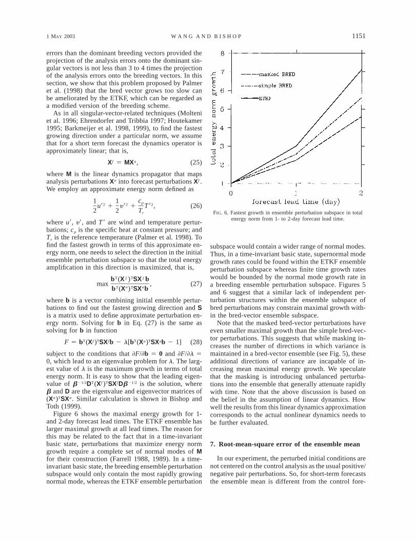
FIG. 6. Fastest growth in ensemble perturbation subspace in totalenergy norm from 1- to 2-day forecast lead time.

errors than the dominant breeding vectors provided theprojection of the analysis errors onto the dominant sin-gular vectors is not less than 3 to 4 times the projectionof the analysis errors onto the breeding vectors. In thissection, we show that this problem proposed by Palmeret al. (1998) that the bred vector grows too slow canbe ameliorated by the ETKF, which can be regarded asa modified version of the breeding scheme.

As in all singular-vector-related techniques (Molteniet al. 1996; Ehrendorfer and Tribbia 1997; Houtekamer1995; Barkmeijer et al. 1998, 1999), to find the fastestgrowing direction under a particular norm, we assumethat for a short term forecast the dynamics operator isapproximately linear; that is,

f aX 5 MX , (25)

where M is the linear dynamics propagator that mapsanalysis perturbations Xa into forecast perturbations Xf .We employ an approximate energy norm defined as

c1 1 p2 2 2u9 1 y9 1 T9 , (26)2 2 Tr

where u9, y9, and T9 are wind and temperature pertur-bations; cp is the specific heat at constant pressure; andTr is the reference temperature (Palmer et al. 1998). Tofind the fastest growth in terms of this approximate en-ergy norm, one needs to select the direction in the initialensemble perturbation subspace so that the total energyamplification in this direction is maximized, that is,

T Tf fb (X ) SX bmax , (27)

a aT Tb (X ) SX b

where b is a vector combining initial ensemble pertur-bations to find out the fastest growing direction and Sis a matrix used to define approximate perturbation en-ergy norm. Solving for b in Eq. (27) is the same assolving for b in function

T T T Tf f a aF 5 b (X ) SX b 2 l[b (X ) SX b 2 1] (28)

subject to the conditions that ]F/]b 5 0 and ]F/]l 50, which lead to an eigenvalue problem for l. The larg-est value of l is the maximum growth in terms of totalenergy norm. It is easy to show that the leading eigen-value of b21/2DT(Xf )TSXfDb21/2 is the solution, whereb and D are the eigenvalue and eigenvector matrices of(Xa)TSXa. Similar calculation is shown in Bishop andToth (1999).

Figure 6 shows the maximal energy growth for 1-and 2-day forecast lead times. The ETKF ensemble haslarger maximal growth at all lead times. The reason forthis may be related to the fact that in a time-invariantbasic state, perturbations that maximize energy normgrowth require a complete set of normal modes of Mfor their construction (Farrell 1988, 1989). In a time-invariant basic state, the breeding ensemble perturbationsubspace would only contain the most rapidly growingnormal mode, whereas the ETKF ensemble perturbation

subspace would contain a wider range of normal modes.Thus, in a time-invariant basic state, supernormal modegrowth rates could be found within the ETKF ensembleperturbation subspace whereas finite time growth rateswould be bounded by the normal mode growth rate ina breeding ensemble perturbation subspace. Figures 5and 6 suggest that a similar lack of independent per-turbation structures within the ensemble subspace ofbred perturbations may constrain maximal growth with-in the bred-vector ensemble subspace.

Note that the masked bred-vector perturbations haveeven smaller maximal growth than the simple bred-vec-tor perturbations. This suggests that while masking in-creases the number of directions in which variance ismaintained in a bred-vector ensemble (see Fig. 5), theseadditional directions of variance are incapable of in-creasing mean maximal energy growth. We speculatethat the masking is introducing unbalanced perturba-tions into the ensemble that generally attenuate rapidlywith time. Note that the above discussion is based onthe belief in the assumption of linear dynamics. Howwell the results from this linear dynamics approximationcorresponds to the actual nonlinear dynamics needs tobe further evaluated.

7. Root-mean-square error of the ensemble mean

In our experiment, the perturbed initial conditions arenot centered on the control analysis as the usual positive/negative pair perturbations. So, for short-term forecaststhe ensemble mean is different from the control fore-


FIG. 7. Globally averaged ensemble mean forecast error (200, 500,and 850 hPa) in terms of the approximate energy norm as a functionof forecast lead time. The corresponding measurement of controlforecast error is also shown as a comparison.

cast.4 The ensemble means are validated against theNCEP–NCAR reanalysis data at 1-, 2-, 3-, . . . , 10-dayforecast lead time at the observation sites. In Fig. 7 weplot the 200-, 500-, and 850-hPa globally averaged en-semble mean forecast error in terms of the approximateenergy norm defined in section 6 [Eq. (26)]. The cor-responding measurements of control forecast errors arealso shown for comparison. It turns out that the ETKFensemble mean is more accurate than both the simplebreeding and the masked breeding for 1-day through10-day forecasts. The ensemble mean of the maskedbreeding is only slightly more skillful than that of thesimple breeding. Compared to the control, the ETKFensemble mean is more accurate than the control for 1-day through 10-day forecasts while the breeding ensem-ble means are only more accurate than the control after4-day forecast. The more accurate ETKF ensemblemean indicates that the ETKF initial perturbations sam-ple the analysis errors better than both breedingschemes. This can be explained by the fact that theETKF samples analysis errors in much more orthogonaland uncorrelated directions than do the breedingschemes (Fig. 5). Calculations on the correlations (notshown here) of the forecast errors from ensemble mem-bers show that the forecast errors of the ETKF ensemblemembers are less correlated than those of both maskedand simple breeding ensemble members.

4 Comparison on paired and unpaired forecasts for a given com-putational expense is carried out in a forthcoming paper.

8. Comparison of ensemble predictions ofinnovation variance

a. Concept of ensemble spread precision

Studies by Toth et al. (2001) and Zhu et al. (2002)suggest that evaluating the ability of an ensemble topredict case-dependent forecast uncertainty is a criticalcriterion to evaluate an ensemble forecast system. Justlike the true state can be regarded as a random variablearound the forecast, the true forecast error variance canbe regarded as a random variable around the ensemblevariance. An accurate prediction of forecast error var-iance is one in which the true forecast error variancedistributes closely to the ensemble variance, that is, thevariance of the forecast error variance around the en-semble variance is small. We refer to the ability of anensemble to get forecast error variance right on everyday at every grid point variable as ‘‘the precision’’ ofthe ensemble variance.

As we shall discuss in future work, information aboutthe degree of ensemble variance precision can be usedto increase the accuracy of error probability densityfunctions derived from ensemble variances. Here, weintroduce new tests of ensemble variance precision.Tests such as rank histograms (Hamill 2001), the relativeoperating characteristics (ROC) curve (Mason 1982;Richardson 2000), and the Brier Skill Score (Brier 1950;Atger 1999) will not be considered here because theyrequire a PDF to be derived from the ensemble forecastand, in our view, the derivation of such PDFs is non-trivial. [Note that the simple method of constructingPDFs by assuming that each ensemble member repre-sents a random draw from the distribution of true fore-casts is inappropriate for ETKF perturbations. As shownin Eqs. (23) and (24), each ETKF analysis perturbationdivided by has an amplitude equal to one stan-ÏK 2 1dard deviation of the error distribution that occurs in itsdirection. Random perturbations would not be governedby such a constraint. For similar reasons, breeding per-turbations should not be considered to be random either.]Future work will be devoted to the derivation of suchPDFs. The spread–skill correlation is not used because,according to Whitaker and Loughe (1998), even for aperfect ensemble the magnitude of the correlation be-tween spread and skill need not be large.

b. Test 1: Resolved range of innovation variance

Consider a scatterplot of points for which the ordinateand abscissa of each point is respectively given by thesquared 500-hPa U wind innovation and 500-hPa Uwind ensemble variance at 1-day forecast lead time atone midlatitude observation location.5 Points collectedcorrespond to all midlatitude radiosonde stations and all

5 Examples of similar scatterplots are given in Majumdar et al.(2002).


FIG. 8. This figure is plotted by first drawing a scatterplot (notshown) of squared 500-hPa U wind innovation vs 500-hPa U windensemble variance at a particular forecast lead time for each mid-latitude observation location for all forecasts during boreal summerof 2000, dividing the points into four equally populated bins, arrangedin order of increasing ensemble variance, and then averaging thesquared innovation and ensemble variance in each bin. What is shownis averaged squared innovation vs the averaged ensemble variancefrom 1- to 3-day forecasts.

1-day 500-hPa U forecasts throughout the NorthernHemisphere summer of 2000. To begin, we divide thepoints into four equally populated bins, arranged in or-der of increasing ensemble variance. Then we averagethe squared innovation and ensemble variance in eachbin, respectively. Connecting the points correspondingto these average values then yields a curve describingthe relationship between the sample innovation varianceand the ensemble variance. Figure 8 provides examplesof such curves.

To interpret the curves in Fig. 8, note that if forecasterrors were uncorrelated with observation errors theninnovation variance would be equal to the sum of fore-cast error variance and observation error variance. Thus,if observation error variance and model errors were alsouncorrelated with forecast error variance6 and if the en-semble variance were equal to the forecast error vari-ance, this curve would be a straight line with a slopeof 458. However, when the true forecast error varianceis a random variable distributed about the given ensem-ble variance then the slope would be less than 458.

To see that inaccurate predictions of forecast errorvariance tend to lead to relatively small slopes, note thatif the ensemble variance were uncorrelated with inno-

6 Note that the variance of the error of representation (often in-cluded in observation error variance estimates) and model error areboth likely to be correlated with forecast error variance.

vation variance then the innovation variances would bethe same for all values of the ensemble variance. In sucha situation, relatively small ensemble variances wouldunderpredict innovation variance, whereas relativelylarge ensemble variances would overpredict innovationvariance. Thus, we expect inaccurate predictions of fore-cast error variance corresponding to relatively small(large) ensemble spread to be negatively (positively)biased. As the accuracy of ensemble-based predictionsof forecast error variance improves, this spread-depen-dent bias will diminish, and the range of innovationvariances distinguishable from ensemble variance willincrease. Thus, by observing the range of the sampleinnovation variance in such plots, the degree of ensem-ble–spread precision is indicated.

Lines in Fig. 8 demonstrate the relationship betweenthe sample innovation variance and the ensemble var-iance for 500-hPa U for 1–3-day forecasts (curves for4–10 days are not shown), where we consider fourequally populated bins with about 2800 points in eachbin. The ETKF ensemble variance can resolve a widerrange of innovation variance than both breeding meth-ods.7 This result is further confirmed when we increasethe number of bins to 64 (;175 points in each bin).The dashed curves in Fig. 9 are the relationship betweenthe sample innovation variance and the ensemble var-iance for 500-hPa U for 2-day forecasts when the num-ber of bins increases to 64. Revealed by the dashedcurves, the range of the sample innovation variancefrom the ETKF ensemble is about 40% and 100% great-er than those from the masked breeding and the simplebreeding ensembles, respectively. When the ensemblevariance is larger than 15 (m s21)2, both the simplebreeding and masked breeding completely lose theirability to distinguish differing forecast error variances.Even for a 9-day forecast lead time, the 64-bin ETKFdashed curve (see dashed curves in Fig. 10) allows in-novation variance to be distinguished over a 17% largerrange than either of the corresponding breeding curves.

c. Test 2: Sensitivity to bin size

If the variance of the true forecast error variance aboutthe ensemble variance is large, then as the sample sizein each bin is reduced the relationship between the sam-ple innovation variance and the ensemble variance be-comes noisier. Thus, the rate at which this relationshipbecomes noisy as the sample size in each bin is reducedis another crude estimate of the accuracy of forecasterror variance prediction method. Figure 9 shows sucha sensitivity test for the 500-hPa U at 2-day forecastlead time. The solid line corresponds to 4 bins of about2800 realizations in each bin while the dashed line cor-responds to 64 bins of about 175 realizations in each

7 Note that the variations of the slopes for each curve are expectedto be because the forecast error variance could correlate with themodel errors and/or the error of representations in observations.


FIG. 9. Sensitivity test on relationship in Fig. 8 to bin size for 2-day forecast lead time for (a) 16-member ETKFensemble, (b) 16-member simple breeding ensemble, and (c) 16-member masked breeding ensemble. The R-squarevalues are shown on right bottom.

bin. The R-square values for the dashed curve relativeto the solid curve are 0.78, 0.65, and 0.49 for the ETKF,masked breeding, and simple breeding ensembles, re-spectively. Thus, as the sample size in each bin is de-creased from 2800 to 175, the relationship between thepredicted and the realized innovation variance becomesthe noisiest for the simple breeding ensemble. As theforecast lead time goes up to 9 or 10 days, the R-squarevalues for the three ensemble methods become similar(see Fig. 10 for 9-day forecast). As mentioned above,even in this case, the 64-bin ETKF curve for the 9-dayforecast still allows innovation variance to be distin-guished over a larger range than either of the corre-sponding breeding curves.

d. Test 3: Kurtosis

Consider a distribution of innovations correspondingto a single value of ensemble variance. Assume that theinnovations are normally distributed with variance equalto the sum of the forecast error variance and observationerror variance. An accurate ensemble variance wouldbe equal to the forecast error variance for all of theinnovation realizations and the distribution of innova-tions corresponding to the ensemble variance valuewould be normally distributed. However, if the ensem-ble-based forecast error prediction was inaccurate, thenthe innovation realizations would correspond to a dis-tribution of forecast error variances. In particular, it


FIG. 10. As in Fig. 9, except for 9-day forecast lead time.

would be likely that innovations corresponding to in-novation variances substantially larger than the mean ofthe innovation variances would occur. Consequently, thelikelihood of finding innovations with extremely largemagnitude within the distribution would increase. Asimple measure of the distribution that is sensitive tosuch extreme values is the kurtosis. The kurtosis is theexpected value of the fourth power of realizations nor-malized by their standard deviation (Goedicke 1953).The kurtosis tends to be larger for distributions withrelatively heavy tails (i.e., many extreme values) thanit is for distributions with thin tails. For a normallydistributed random variable, the kurtosis is equal to 3.For finite sample sizes, the true mean and kurtosis areunknown. Nevertheless, one can approximate them withthe sample mean and the sample kurtosis. We first cal-

culate the innovation kurtosis in each of the four bins(about 2800 innovations in each bin) and then averagethe four kurtosis values. Figure 11 shows the 500-hPaU innovation kurtosis averaged over four bins as a func-tion of forecast lead time. The ETKF kurtosis is smallerthan that of both the breeding methods throughout 1-to 10-day forecasts.

We conclude this section by noting that the resultsfrom all three of our ensemble precision measures in-dicate that the ETKF ensemble variance is more accuratethan the ensemble variances produced by the breedingensembles.

9. Computational expenseThe main computations required for the ETKF

scheme are the (K 2 1) 3 (K 2 1) inner products in


FIG. 11. Innovation kurtosis for 500-hPa U averaged on four binsdefined in Fig. 8 for 1- to 10-day forecast lead time.

observation space required to form the elements of(Z f )THTR21HZf [Eq. (10)] together with its eigenvectordecomposition. Because K is the number of ensemblemembers, the number of operations required for thesecomputations is much less than that required for thegeneration of the singular vector perturbations (Molteniet al. 1996) and the perturbed observation perturbations(Houtekamer et al. 1996). In our experiment, the com-putational expense for generating the ETKF initial per-turbations is only 6% and 4% more expensive than thatof generating the simple breeding and masked breedinginitial perturbations, respectively.

10. Summary

The ETKF ensemble generation technique is similarin spirit to the breeding technique in that it views anal-ysis perturbations as filtered forecast perturbations. In-stead of multiplying each forecast perturbation a globalor regional rescaling factor, the ETKF ensemble gen-eration scheme transforms forecast perturbations intoanalysis perturbations via linear combinations of fore-cast perturbations that solve the error variance updateequation for the optimal data assimilation within theensemble perturbation subspace. Consequently, theETKF analysis perturbation is able to reflect the densityand accuracy of observations. Although the breedingmodulated by a mask seems able to resolve the spatialinhomogenieties of the observation distribution, themask is only two-dimensional and time invariant. Be-sides, it can produce initial perturbation imbalance thatexcites unrealistic wave growth. Provided 12-h forecastperturbations are balanced and of linear amplitude then

the ETKF analysis perturbations are balanced. In theETKF scheme, directions corresponding to large fore-cast error variance in observation space are attenuatedmore than directions corresponding to small forecasterror variance. Thus, while the error variance of a 16-member breeding ensemble is concentrated in a singledirection, the ETKF 16-member ensemble error vari-ance was spread with comparable amounts among 15independent, orthogonal, and uncorrelated directions.The application of a mask on the breeding only slightlyameliorates the rank deficiency problem of the simplebreeding method.

The fastest growth under the energy norm within theensemble perturbation subspace of the ETKF scheme islarger than the breeding schemes. The application of themask actually degrades the fastest growth rate of thesimple breeding scheme. The ensemble mean of theETKF ensemble is more accurate than both breedingmethods. It is argued that imperfections in the corre-spondence between ensemble variance and forecast er-ror variance would be indicated by (a) a relatively smallrange over which sample pseudoinnovation variancecould be predicted from ensemble variance, (b) a highsensitivity of the relationship between ensemble vari-ance and sample pseudoinnovation variance to the num-ber of realizations in each bin, and (c) distributions with-in each bin of pseudoinnovations whose mean fourthpowers (kurtosis) are relatively high (see section 8b forthe definition of a bin). Investigation along these linesindicates that the ETKF estimates of forecast error var-iance are considerably more accurate than those of thebreeding techniques. In other words, the ensemblespread of the ETKF ensemble is better able to distin-guish the case-to-case forecast uncertainty than thebreeding ensembles.

Besides the superior ensemble forecast skills of theETKF scheme over the breeding schemes, the compu-tational expense of the ETKF is also quite small (,6%more than the breeding ensemble). Thus, the ETKF en-semble generation scheme would be straightforward toemploy operationally. When applied to operational fore-cast centers, more ensemble members and more realisticobservation networks need to be included.

Acknowledgments. The authors gratefully acknowl-edge financial support from Pennsylvania, Power andLight, ONR Grant N00014-00-1-0106 and ONR ProjectElement 0601153N, Project Number BE-033-0345. It isdoubtful that our integrations could have been per-formed without the generous and expert computationalassistance of Robert Hart, Vijay Agarwala, and Jan Dut-ton. Frank Peacock also made important contributionsat the early stages of this work. Thanks also goes toTom Hamill and one anonymous reviewer for their pa-tient and thoughtful reviews.


APPENDIX

Filtering Effect of Optimal Data Assimilation

For an optimal data assimilation scheme, analysis er-ror covariance matrix Pa is related to the forecast errorcovariance matrix Pf and observation error covariancematrix R by

21a f f T f T fP 5 P 2 P H (HP H 1 R) HP , (A1)

where H is the linear observation operator that maps modelvariables to observed variables. Define H̃ 5 R21/2H. Thenpremultiply and postmultiply (A1) by H̃ and H̃T, re-spectively. Then (A1) becomes

a 21T f T f T f T f T˜ ˜ ˜ ˜ ˜ ˜ ˜ ˜ ˜ ˜HP H 5 HP H 2 HP H (HP H 1 I) HP H ,(A2)

where I is the identity matrix; H̃PaH̃T/H̃PfH̃T is the anal-ysis/forecast error covariance matrix in the observationsubspace and normalized by the observation error co-variance. To see the filtering effect, we express (A2) interms of the eigenvectors of H̃PfH̃T. Suppose each col-umn of E is an eigenvector of H̃PfH̃T, and G is a diagonalmatrix containing corresponding eigenvalues of H̃PfH̃T.Then

f T T˜ ˜HP H 5 EGE , and (A3)21 21f T T˜ ˜(HP H 1 I) 5 E(G 1 I) E . (A4)

Using (A3) and (A4), (A2) becomes2 21 21a T T T˜ ˜HP H 5 E[G 2 G (G 1 I) ]E 5 EG(G 1 I) E .

(A5)

Comparing Eqs. (A3) and (A5), error variance on theith eigenvector is reduced by multiplying a factor 1/(li

1 1), where l i is the ith eigenvalue. Thus, error variancein the direction of the leading eigenvector is attenuatedthe most. Consequently, the eigenvalue spectrum ofH̃PaH̃T is whiter than that of H̃PfH̃T.

REFERENCES

Anderson, J. L., 2001: An ensemble adjustment Kalman filter for dataassimilation. Mon. Wea. Rev., 129, 2884–2903.

Atger, F., 1999: The skill of ensemble prediction systems. Mon. Wea.Rev., 127, 1941–1953.

Barkmeijer, J., M. van Gijzen, and F. Bouttier, 1998: Singular vectorsand estimates of the analysis error covariance metric. Quart. J.Roy. Meteor. Soc., 124, 1695–1713.

——, R. Buizza, and T. N. Palmer, 1999: 3D-Var Hessian singularvectors and their potential use in the ECMWF ensemble pre-diction system. Quart. J. Roy. Meteor. Soc., 125, 2333–2351.

Bishop, C. H., and Z. Toth, 1999: Ensemble transformation and adap-tive observations. J. Atmos. Sci., 56, 1748–1765.

——, B. J. Etherton, and S. J. Majumdar, 2001: Adaptive samplingwith the ensemble transform Kalman filter. Part I: Theoreticalaspects. Mon. Wea. Rev., 129, 420–436.

——, C. A. Reynolds, and M. K. Tippett, 2003: Optimization of thefixed global observing network in a simple model. J. Atmos. Sci.,in press.

Brier, G. W., 1950: Verification of forecasts espressed in terms ofprobabilities. Mon. Wea. Rev., 78, 1–3.

Buizza, R., and T. N. Palmer, 1995: The singular-vector structure ofthe atmospheric global circulation. J. Atmos. Sci., 52, 1434–1456.

Cohn, S. E., and D. P. Dee, 1988: Observability of discretized partialdifferential equations. Siam. J. Numer. Anal., 25, 586–617.

Daley, R., 1991: Atmospheric Data Analysis. Cambridge UniversityPress, 457 pp.

Dee, D. P., 1995: On-line estimation of error covariance parametersfor atmospheric data assimilation. Mon. Wea. Rev., 123, 1128–1196.

Ehrendorfer, M., and J. J. Tribbia, 1997: Optimal prediction of fore-cast error covariances through singular vectors. J. Atmos. Sci.,54, 286–313.

Farrell, B. F., 1988: Optimal excitation of neutral Rossby waves. J.Atmos. Sci., 45, 163–172.

——, 1989: Optimal exictation of baroclinic waves. J. Atmos. Sci.,46, 1193–1206.

Goedicke, V. A., 1953: Introduction to the Theory of Statistics. Ac-ademic Press, 286 pp.

Hamill, T. M., 2001: Interpretation of rank histograms for verifyingensemble forecasts. Mon. Wea. Rev., 129, 550–560.

——, and C. Snyder, 2000: A hybrid ensemble Kalman filter–3Dvariational analysis scheme. Mon. Wea. Rev., 128, 2905–2919.

——, ——, and R. E. Morss, 2000: A comparison of probabilisticforecasts from bred, singular vector, and perturbed observationensembles. Mon. Wea. Rev., 128, 1835–1851.

——, J. S. Whitaker, and C. Snyder, 2001: Distance-dependent fil-tering of background error covariance estimates in an ensembleKalman filter. Mon. Wea. Rev., 129, 2776–2790.

——, C. Snyder, and J. S. Whitaker, 2003: Ensemble forecasts andthe properties of flow-dependent analysis-error covariance sin-gular vectors. Mon. Wea. Rev., in press.

Houtekamer, P. L., 1995: The construction of optimal perturbations.Mon. Wea. Rev., 123, 2888–2898.

——, and J. Derome, 1995: Methods for ensemble prediction. Mon.Wea. Rev., 123, 2181–2196.

——, and H. L. Mitchell, 1998: Data assimilation using an ensembleKalman filter technique. Mon. Wea. Rev., 126, 796–811.

——, and ——, 2001: A sequential ensemble Kalman filter for at-mospheric data assimilation. Mon. Wea. Rev., 129, 123–137.

——, L. Lefaivre, J. Derome, H. Ritchie, and H. L. Mitchell, 1996:A system simulation approach to ensemble prediction. Mon.Wea. Rev., 124, 1225–1242.

Ide, K., P. Courtier, M. Ghil, and A. C. Lorenc, 1997: Unified notationfor data assimilation: Operational, sequential, and variational. J.Meteor. Soc. Japan, 75, 181–189.

Jeffery, T. K., J. H. Hack, B. B. Gordon, B. A. Boville, B. P. Briegleb,D. L. Williamson, and P. J. Rasch, 1996: Description of theNCAR community climate model (CCM3). NCAR Tech. NoteNCAR/TN-4201STR, 152 pp.

Kalman, R., 1960: A new approach to linear filtering and predictedproblems. J. Basic Eng., 82, 35–45.

——, and R. Bucy, 1961: New results in linear filtering and predictiontheory. J. Basic Eng., 83, 95–105.

Kleeman, R., 1989: A modeling study of the effect of the Andes onthe summertime circulation of tropical South America. J. Atmos.Sci., 46, 3344–3362.

Leith, C. E., 1974: Theoretical skill of Monte Carlo forecasts. Mon.Wea. Rev., 102, 409–418.

Majumdar, S. J., C. H. Bishop, and B. J. Etherton, 2002: Adaptivesampling with the ensemble transform Kalman filter. Part II:Field program implementation. Mon. Wea. Rev., 130, 1356–1369.

Mason, I. B., 1982: A model for the assessment of weather forecasts.Aust. Meteor. Mag., 30, 291–303.

McPhaden, M. J., and A. E. Gill, 1987: Topographic scattering ofequatorial waves. J. Phys. Oceanogr., 17, 82–96.

Molteni, F., R. Buizza, T. N. Palmer, and T. Petroliagis, 1996: TheECMWF ensemble prediction system: Methodology and vali-dation. Quart. J. Roy. Meteor. Soc., 122, 73–119.


Palmer, T. N., R. Gelaro, J. Barkmeijer, and R. Buizza, 1998: Singularvectors, metrics, and adaptive observations. J. Atmos. Sci., 55,633–653.

Richardson, D. S., 2000: Skill and economic value of the ECMWFensemble prediction system. Quart. J. Roy. Meteor. Soc., 126,649–669.

Sardeshmukh, P., and B. J. Hoskins, 1984: Spatial smoothing on thesphere. Mon. Wea. Rev., 112, 2524–2529.

Tippett, M. K., J. L. Anderson, C. H. Bishop, T. M. Hamill, and J.S. Whitaker, 2003: Ensemble square root filters. Mon. Wea. Rev.,in press.

Toth, Z., and E. Kalnay, 1993: Ensemble forecasting at NMC: Thegeneration of perturbations. Bull. Amer. Meteor. Soc., 74, 2317–2330.

——, and ——, 1997: Ensemble forecasting at NCEP and the breed-ing method. Mon. Wea. Rev., 125, 3297–3319.

——, Y. Zhu, and T. Marchok, 2001: The use of ensembles to identifyforecasts with small and large uncertainty. Wea. Forecasting,16, 436–477.

Whitaker, J. S., and A. F. Loughe, 1998: The relationship betweenensemble spread and ensemble mean skill. Mon. Wea. Rev., 126,3292–3302.

——, and T. M. Hamill, 2002: Ensemble data assimilation withoutperturbed observations. Mon. Wea. Rev., 130, 1913–1924.

Zhu, Y., Z. Toth, R. Wobus, D. Richardson, and K. Mylne, 2002: Theeconomic value of ensemble-based weather forecasts. Bull.Amer. Meteor. Soc., 83, 73–83.

a comparison of breeding and ensemble transform...

Documents