a comparison of gradient estimation methods for volume

1

A Comparison of Gradient Estimation Methods for VolumeRendering on Unstructured Meshes

Carlos D. Correa, Member, IEEE, Robert Hero, and Kwan-Liu Ma, Senior Member, IEEE

Abstract—This paper presents a study of gradient estimation methods for rendering unstructured-mesh volume data. Gradientestimation is necessary for rendering shaded isosurfaces and specular highlights, which provide important cues for shape and depth.Gradient estimation has been widely studied and deployed for regular-grid volume data to achieve local illumination effects, but hasbeen otherwise for unstructured-mesh data. As a result, most of the unstructured-mesh volume visualizations made so far were unlit.In this paper, we present a comprehensive study of gradient estimation methods for unstructured meshes with respect to their costand performance. Through a number of benchmarks, we discuss the effects of mesh quality and scalar function complexity in theaccuracy of the reconstruction, and their impact in lighting-enabled volume rendering. Based on our study, we also propose twoheuristic improvements to the gradient reconstruction process. The first heuristic improves the rendering quality with a hybrid algorithmthat combines the results of the multiple reconstruction methods, based on the properties of a given mesh. The second heuristicimproves the efficiency of its GPU implementation, by restricting the computation of the gradient on a fixed-size local neighborhood.

Index Terms—Volume rendering, Gradient estimation, Local Illumination, Unstructured meshes, Flow visualization.

✦

1 INTRODUCTION

LIGHTING plays an important role in volume rendering.On one hand, shading and specular reflections provide

important cues of shape and depth. On the other hand,diffuse shading along the contours of an isosurface helpsdisambiguate the overlapping structures that are common insemi-transparent rendering. For example, Fig. 1 shows theresult of applying local illumination to two volumes sampledin unstructured meshes. On the left, lighting helps discoverturbulent patterns that are lost in the unlit image. On the right,lighting helps elucidate the spatial relationships between theoccluding isosurfaces. Without it, isosurfaces appear flat withno apparent depth disambiguation.

To properly apply local illumination to a 3D volume, wemust estimate the gradient of the volume accurately at ev-ery single point, while hiding the effects of mesh resolution,which introduce undesired artifacts. Gradient estimation iswell known and understood for regular grids, and its ap-plication is now part of commodity visualization systems.Due to the structured nature of regular grids, estimating thegradient is a rather simple task. The partial derivatives of afunction with respect to the X,Y and Z dimensions are easilyapproximated using finite differences given the alignment ofa voxel neighborhood with each of the axes. Unstructuredmeshes do not provide the same advantage. Usually based onfinite element methods, these grids are used to discretize ascalar or vector field within a closed volume using a variety ofcell types, such as tetrahedra, hexahedra and prisms. The useof cells of varying shape and size enables a better fit of the gridwith complex geometries and adaptive refinement in regionsof interest. Unstructured meshes, with the exception of anunstructured cloud of points, contain connectivity informationthat may be used to compute the gradient. However, it is not asstraightforward as in regular grids. First, connected vertices do

• The authors are with the Visualization and Interface Design Innovation(VIDI) Research Group, Department of Computer Science, University ofCalifornia, 2063 Kemper Hall, One Shields Avenue, Davis, CA 95616.E-mail: [email protected], [email protected], [email protected]

not align with the main axes, suggesting a variable contribu-tion to each component of the gradient. Second, unstructuredmeshes usually contain elements of varying shape, where onedimension is better sampled than the others. The traversal ofthis connectivity is somewhat costly when compared to theconvolution step usually required for structured grids. Evenwith no connectivity, computing a stencil around a given pointdemands a spatial search that may vary in size. For this reason,local illumination of unstructured-mesh volume data has beenlargely ignored. A simple mechanism would be to imposea regular grid and re-sample the volume accordingly, but itresults in sampling problems. Re-sampling an unstructuredmesh into a 3D regular grid at the Nyquist rate might result invery large volumes that exceed the available system or graphicsmemory.

In this paper, we present a comparison and quantitativeanalysis of the most prominent methods for linear gradient re-construction for the purpose of lighting. Although higher orderelements are becoming increasingly available, linear elementsare still the most common representation for unstructuredmeshes, particularly for hardware accelerated rendering sys-tems. The cost of storing and rendering higher order elementshas not made it possible to render them at interactive rates incurrent graphics processing units. Understanding the factorsthat affect the quality of volume rendered images in linearunstructured meshes not only improves current visualizationsystems, but also paves the way for similar studies of higherorder meshes.

We make the following contributions: (1) We present acomprehensive comparison of linear gradient reconstructionmethods on unstructured meshes. Our systematic approachdecomposes the accuracy of the gradient as the product ofdifferent factors, such as mesh resolution, element shape andcomplexity of the scalar field. Our experiments suggest simpleguidelines for applying the appropriate method for a givenunstructured mesh to produce high-quality volume renderedimages. To the best knowledge of the authors, this is thefirst attempt to obtain a comparison of the different gradi-ent estimation methods from the visualization standpoint. (2)Based on our results, we present two heuristic improvements.

Digital Object Indentifier 10.1109/TVCG.2009.105 1077-2626/09/$26.00 © 2009 IEEE

IEEE TRANSACTIONS ON VISUALIZATION AND COMPUTER GRAPHICSThis article has been accepted for publication in a future issue of this journal, but has not been fully edited. Content may change prior to final publication.

2

Fig. 1. Effect of lighting in unstructured-mesh rendering for two data sets. Left: Lighting helps discover turbulent structures in thevicinity of the wing that appear flat otherwise. Proper gradient estimation should highlight these shapes without adding extraneousartifacts. Right: Lighting also helps understand the spatial relationship between different occluding isosurfaces. With lighting, theactual shape of the semi-transparent isosurfaces can be easily perceived even in the presence of overlapping surfaces.

Hybrid gradient reconstruction improves the visual qualityby applying different methods in a single mesh according toa given quality metric. In our experiments, regression-basedmethods behave better for irregular elements in comparisonto methods based on averaging, and vice versa for regularelements. This suggests that the choice of method shouldfollow the local mesh quality instead of being applied globally.Fixed-size neighborhood gradient reconstruction is anotherheuristic that ranks the neighbor vertices of a given point sothat the gradient can be reconstructed as accurately as possiblewithout incurring in much overhead.

2 RELATED WORK

Volume rendering of unstructured meshes has become an im-portant tool for understanding computational fluid dynamicsand mesh discretizations of PDEs. The most predominant ren-dering approaches are cell projection [27], point-based approaches[32], [34] and raycasting [11], [30]. For its simplicity, some practi-tioners re-sample the unstructured mesh into a regular grid andrender this grid directly [29], [31]. GPU-based implementationsof these methods exist [9], [18], [30]. Cell projection and point-based approaches, often classified as object-order approaches,do not require an explicit connectivity of the cells. However,they require visibility sorting. Image-order approaches, suchas raycasting, do not require visibility sorting, but they requirethe connectivity information to traverse the cells along the viewrays. In this paper, we use raycasting to test our results andprovide a visual comparison. Our implementation is based onthe ones by Garrity [11] and Weiler et al. [30]. The methods de-scribed in this paper and the results of our evaluation, however,are applicable to both object- and image-order approaches.

The study of gradients in unstructured meshes can beunderstood from both the simulation and the visualizationstandpoints. In simulation, the study of gradient reconstruc-tion methods leads to more accurate reconstructions of anunderlying scalar function and better error bounds for thediscretization of PDEs. Most of these studies rely on meth-ods based on linear regression and the Green-Gauss theorem[7], [19], [17]. Aftosmis et al. discuss the behavior of linearreconstruction methods on unstructured meshes [3]. In theirstudies, Barth [7], Mavriplis [17] and Anderson [5] found thatinverse distance weighting has a significant impact on linearregression models for gradient estimation, while methods suchas Green-Gauss degrade. In an attempt to improve the er-ror bounds of gradient reconstruction, Shewchuk studies theimpact of cell shape in linear reconstruction and provides aseries of quality metrics for tetrahedral cells [26]. Petrovskaya

[25] and Apel et al. [6] also study the impact of cell shapein reconstruction algorithms. While there is no consensus onwhat is a good mesh element, these studies suggest thatthese methods produce noticeable differences in the gradientreconstruction as the mesh becomes more irregular. In thispaper, we aim at validating some of these findings from therendering standpoint.

In visualization, gradient estimation becomes important asshading is an essential cue for shape. For geometric objects,such as triangle meshes, normals to the surface can be com-puted directly from the geometric representation. Volume rep-resentations, however, do not encode explicit geometry but aresampled in a grid or an unstructured mesh. The gradient isnot computed directly from the geometric information, butrequires the consideration of the volume data. Yagel et al.surveys these methods for structured grids and classifies theminto image-space and object-space methods [33]. With the ad-vent of fast graphics processors, object-space methods becamethe norm. Moller et al. compare normal estimation schemesfrom the point of view of the quality of the reconstructionfilter [20]. A similar study is carried out by Bentum et al.in the frequency domain [8]. In the spirit of generalization,Thurmer and Wuthrich consider the normal computation in 3Dspace as an approximation resulting from sampling a spatialneighborhood of each point, and describe the importance ofvariable weighting of each sample [28]. Neumann et al. alsoconsider the problem around a neighborhood and pose theproblem as 4D regression [22]. Although these two methodswere described for structured grids, their derivations alsoapply to unstructured meshes. While not designed for volumerendering, the need for reconstructing smooth functions fromunorganized points has emerged in the point-based renderingcommunity. Estimating the gradient to a surface has beenposed as a total least squares problem [12] or a moving leastsquares problem [24]. Similar techniques can be applied whenwe consider an unstructured mesh as a collection of points.

Cell-based gradient estimation was proved useful in visual-ization to speed up the sampling of the scalar fields at arbi-trary points within a cell. This was first proposed by Garrity[11], who estimated the constant cell gradient via a linearapproximation. This was later used by Weiler et al. in GPU-based raycasting [30]. A constant cell gradient, however, is notadequate for lighting, and node-centered gradients are needed.Cignoni et al. use the average of the gradient of the incidentcells to compute the gradient at a node [10], and use it to rendershaded isosurfaces. Ma et al. compute the gradient based onan approximation of the Green-Gauss theorem [15], which was


3

later modified by Meredith and Ma, who use the directionalderivatives of the scalar field to obtain a fast approximation[18]. Levy et al. use unweighted linear regression to estimatethe normals [14]. We show that weighted regression providesa better estimate of the gradient than unweighted schemes. Inrecent approaches, the lack of lighting is compensated withopacity transformations, which result in an appearance similarto shaded isosurfaces [21].

This heterogeneity of methods in both the simulation andthe visualization communities demonstrates that there is noconsensus on what are the most adequate methods for addinglighting to volume data in unstructured meshes. In this paper,we provide a quantitative and qualitative evaluation of themost prominent linear gradient reconstruction methods. Weseek to guide future generations of unstructured mesh visu-alization systems towards high-quality volume rendering.

3 LINEAR GRADIENT RECONSTRUCTION

Let us define an unstructured mesh as a collection of connectedpoints x that discretize a scalar field f . The linear approxima-tion of this function at a given point x0 + h is given by

f(x0 + h) = f(x0) +∇f(x0) · h + O(||h||2) (1)

where ∇(f(x0) is the gradient at point x0 and h is a discretiza-tion step. The goal of gradient estimation is therefore to recoverthe function ∇f such that Eq. (1) holds for any given point.Because the approximation is linear, these methods are collec-tively known as linear gradient reconstruction methods. Wecan further classify these methods into two groups: averaging-based methods, which construct the gradient as a weightedaverage of the neighboring gradients, and regression-basedmethods, which posit Eq. (1) as a least squares problem.

To understand the sources of error in these methods, wecan expand the second term of the linear approximation. Theresidual of r2 = f − f , where f is the linear approximation off , is

r2(x0 + h) =1

2!h�∇2f(x0)h + O(||h||3) (2)

where ∇2f is the Hessian matrix of f . Furthermore, the abso-lute error can be bounded as:

||r2|| ≤ ||h||2||∇2(f(ξ, ζ, η))|| (3)

for some (ξ, ζ, η)� ∈ (x0,x0 +h). Therefore, linear approxima-tion methods are both dependent on the mesh discretizationand the complexity of the scalar field. This is true for bothstructured and unstructured meshes. Unlike structured grids,unstructured meshes have a variable discretization distanceh. Therefore, the shape of the mesh element is also a factor.Numerous quality metrics have been proposed for tetrahedra,as described in [26]. The study of these metrics, of which themost common are aspect ratio and the ratio of the inscribingsphere and maximum edge length, has led to tighter boundson the approximation error [6]. Here, we are not concernedabout these bounds, but rather in the effects of the differentfactors in the volume rendered image. Mavriplis showed thatregression-based methods provide better estimates on irregularelements rather than averaging-based methods [17]. Shewchukalso notes that this effect has been misunderstood as due toelements of poor aspect ratio, but argues that it is the presenceof large angles that results in larger approximation error. In ourvisual analysis, we show how the different methods behavedifferently depending on the element shape.

3.1 Averaging Based Methods

In this family of methods, the gradient is computed as aweighted average of functions of the gradient or scalar valuesat a neighborhood around a node. In general, this can beexpressed as the linear combination

∇f(x0) =X

i

wi∇f(i) (4)

where wi is a weighting factor, and ∇f(i) is the constantgradient at a cell i. The gradient at a cell can be computedby considering Eq. (1) for the 4 vertices of a tetrahedron, heredenoted as column vectors x0, x1, x2 and x3, resulting in the3× 3 linear system2

4 (x1 − x0)�

(x2 − x0)�

(x3 − x0)�

35∇f =

24 f(x1)− f(x0)

f(x2)− f(x0)f(x3)− f(x0)

35 (5)

The left hand side consists of a 3 × 3 matrix where each rowis a displacement and the three columns are the componentsin each of the spatial dimensions. The right hand side is acolumn vector of scalar differentials. This system can be solvedexactly for non-degenerate tetrahedra, i.e., tetrahedra that donot collapse into a plane, a line or a point.

3.1.1 Cell Weighting

Since the cells around a given vertex are not of the sameshape, the weighting factors wi can be computed to give higherimportance to those cells that should contribute more to theaverage gradient (Fig. 2(a)). Here, we consider four methods:

Uniform. This is the case when all cells are weighted uni-formly. This method is the most commonly used in volumerendering due to its simplicity, but does not adapt to meshesof varying shape.

Volume. Each cell is weighted according to its own volume.Although it adapts better to meshes of varying shape, someelements may exhibit small aspect ratio while having the samevolume of other more regular elements. Later on, we show thatthis method is equivalent to obtaining the gradient using theGreen Gauss theorem.

Solid Angle. A cell is weighted by the solid angle subtendedby the cell at the central vertex x0, measured as the surface areaof a unit sphere covered by the opposite face to vertex x0.

Inverse centroid distance. Each cell is weighted by theinverse of the distance between the central vertex x0 and thecentroid of cell i.

3.1.2 Green-Gauss Method

A different derivation of the gradient is obtained using theGreen-Gauss theorem, which states that for a volume Ω en-closed by a surface S,Z

Ω

∇fdΩ =

Z∂Ω

fndS (6)

where n denotes the outward pointing normal vector to thesurface S, as shown in Fig. 2(b). In an unstructured mesh, theaverage gradient at a node can be approximated by

∇f(x0) ≈1

|Ω|

Z∂Ω

fndS (7)

≈1

|Ω|

Xi∈S1,...,Sn

f ini (8)

The first approximation replaces the volume integral of theregion enclosing the vertex by the total volume. The second


4

(a) Cell Average (b) Green Gauss (c) Regression (d) Meshless

Fig. 2. Overview of the gradient estimation methods. (a) Weighted average of the neighboring cell gradients. Typical weights arevolume, solid angle φi or inverse centroid distance 1/||ci − x0||. (b) The Green Gauss method approximates the gradient as thesurface integral of the control volume Ω. (c) Regression fits a plane for the gradient based on the contribution of the direct neighborsof vertex x0. (d) Meshless methods apply regression on scattered points in a spatial neighborhood (e.g., a sphere of radius r).

approximation is done over the surface integral using thetrapezoidal rule on each of the faces Si defining the surface. ni

denotes the outward pointing normal vector of the face Si. Thescalar value at a face, f i, is obtained as the linearly interpolatedscalar value at the barycenter of face Si.

We can see that the Green Gauss method is equivalent tocomputing the volume weighted cell average gradient. Let usdefine the volume integral of the gradient in a neighborhoodof cells around a central vertex x0. Assuming that the gradientat the cell is constant [3],Z

Ω

∇fdΩ =X

i

∇f(i)

ZΩi

dΩ (9)

=X

i

∇f(i)Vi (10)

where Vi is the volume of cell i. That is, if we convert eachelement volume integral into an element Green-Gauss surfaceintegral, the contributions from shared internal faces will cancelout in the summation over the entire region, resulting in theGreen-Gauss approximation.

3.2 Regression Based Methods

Another family of methods can be derived from Eq. (1) byfitting a hyperplane that best satisfies the equation for anumber of sample points, as depicted in Fig. 2(c). In the caseof node-centered gradients, Eq. (1) can be generalized to anover-constrained system of equations.2

6664(x1 − x0)

�

(x2 − x0)�

...(xk − x0)

�

37775∇f =

26664

f(x1)− f(x0)f(x2)− f(x0)

...f(xk)− f(x0)

37775 (11)

(12)

where x1, . . . ,xk are the vertex neighbors of vertex x0. Equiv-alently, this system can be expressed in matrix form,

X∇f = b (13)

where X is a k×3 matrix whose columns are the displacementof each vertex in the spatial dimensions, and b is a columnvector of dimensions k × 1 of scalar value differentials. Theproblem can be solved using linear least squares.

As can be seen, this method extends naturally to arbitraryelement shapes and neighborhoods. In particular, considering

all the vertices in a spatial neighborhood of x0 leads to ameshless gradient reconstruction scheme. The same cannot besaid about averaging methods. As pointed out by Mavriplis,the Green Gauss approximation is generally not exact fordiscretizations other than tetrahedra [17], although differentcontrol volumes can be defined for such cases.

3.2.1 Weighting

To account for the unstructured nature of the mesh, regression-methods can be modified to add weights to each of the vertexneighbors. Let wi denote a weighting factor associated withvertex xi. The gradient reconstruction can be posed as the overconstrained system:

WX∇f = Wb (14)

where W = diag{wi} is a k×k diagonal matrix containing theweights of all k neighbors of vertex xo. The solution to thissystem can be computed using weighted least squares, solvingthe 3× 3 system

X�W

2X∇f = X

�W

2b (15)

With regards to weighting, we consider two cases: unweightedregression, for wi = 1, commonly used in volume rendering,and inverse distance weighted regression, in which case wi =

1||x−x0||2

, where || · || denotes the Euclidean norm of a 3Dvector. Mavriplis showed that, in general, weighted regressionprovides better estimates than unweighted regression, espe-cially for irregular elements [17]. We can see this in the normof the matrix in Eq. (15). The matrix is inherently dependenton the element shape. For irregular elements, the differencein edge lengths generates a large conditioning for the matrix.For unweighted regression, the determinant of X�X grows asO(||h||6) (since it grows as the cube of the elements in thematrix, which are O(||h||2)) and the problem is ill-conditionedfor nearly coplanar cells. Weighting using inverse distancecancels out the dependency on the shape of surroundingtetrahedra, and the determinant of X�W2X grows as O(1), sothat it is less sensitive to near-coplanar cases. This differencein accuracy was observed in our experiments and is consistentwith previous results [17], [25].

3.2.2 4D Regression

As an alternative to 3D regression, Eq. (1) can be formulated asa 4D regression problem, as suggested by Neumann et al. [22].


5

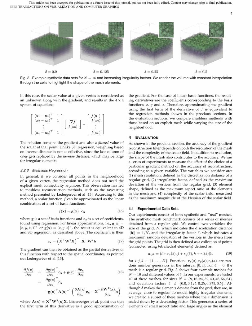
δ = 0.0 δ = 0.125 δ = 0.25 δ = 0.5

Fig. 3. Example synthetic data sets for N = 16 and increasing irregularity factors. We render the volume with constant interpolationthrough the cells to highlight the shape of the mesh elements.

In this case, the scalar value at a given vertex is considered asan unknown along with the gradient, and results in the 4× 4system of equations:

26664

(x1 − x0)� 1

(x2 − x0)� 1

...(xk − x0)

� 1

37775

»∇f

f(x0)

–=

26664

f(x1)f(x2)

...f(xk)

37775

The solution contains the gradient and also a filtered value ofthe scalar at that point. Unlike 3D regression, weighting basedon inverse distance is not as effective, since the last column ofones gets replaced by the inverse distance, which may be largefor irregular elements.

3.2.3 Meshless Regression

In general, if we consider all points in the neighborhoodof a given vertex, the regression method does not need theexplicit mesh connectivity anymore. This observation has ledto meshless reconstruction methods, such as the raycastingmethod presented by Ledergerber et al [13]. According to thismethod, a scalar function f can be approximated as the linearcombination of a set of basis functions:

f(x) = g(x)�cx (16)

where g is a set of basis functions and cx is a set of coefficients,found using regression. For linear approximations, i.e., g(x) =[x, y, z, 1]� or g(x) = [x, y, z]�, the result is equivalent to 4Dand 3D regression, as described above. The coefficient is then

cx =“X

�W

2X

”−1

X�W

2b (17)

The gradient can then be obtained as the partial derivatives ofthis function with respect to the spatial coordinates, as pointedout Ledergerber et al [13].

∂f(x)

∂xk

=∂g(x)

∂xk

�

cx + g(x)�∂cx

∂xk

(18)

=∂g(x)

∂xk

�

cx

−g(x)�A(x)−1

„∂A(x)

∂xk

cx −X� ∂W2(x)

∂xk

b

«

where A(x) = X�W2(x)X. Lederberger et al. point out thatthe first term of this derivative is a good approximation of

the gradient. For the case of linear basis functions, the result-ing derivatives are the coefficients corresponding to the basisfunctions x, y and z. Therefore, approximating the gradientusing the first term of the derivative of f is equivalent tothe regression methods shown in the previous sections. Inthe evaluation sections, we compare meshless methods withthose based on an explicit mesh while varying the size of theneighborhood.

4 EVALUATION

As shown in the previous section, the accuracy of the gradientreconstruction filter depends on both the resolution of the meshand the complexity of the scalar field. In addition to resolution,the shape of the mesh also contributes to the accuracy. We rana series of experiments to measure the effect of the choice of aparticular gradient method on the accuracy of reconstruction,according to a given variable. The variables we consider are:(1) mesh resolution, defined as the discretization distance of aregular grid, (2) irregularity factor, defined as the maximumdeviation of the vertices from the regular grid, (3) elementshape, defined as the maximum aspect ratio of the elementsin the mesh and (4) complexity of the scalar field, measuredas the maximum magnitude of the Hessian of the scalar field.

4.1 Experimental Data Sets

Our experiments consist of both synthetic and “real” meshes.The synthetic mesh benchmark consists of a series of meshesobtained from a regular grid. We control two variables: thesize of the grid, N , which indicates the discretization distance||h|| = 1/N , and the irregularity factor δ, which indicates amaximum random deviation of the vertices in the mesh fromthe grid points. The grid is then defined as a collection of points(connected using tetrahedral elements) defined as:

xijk = (i + rx(δ), j + ry(δ), k + rz(δ))h (19)

for i, j, k ∈ {1, . . . , N}. Functions rx(a), ry(a), rz(a) are ran-dom number generators in the interval [0, a]. For δ = 0, themesh is a regular grid. Fig. 3 shows four example meshes forN = 16 and different values of δ. In our experiments, we tested40 of these meshes, for sizes N = {8, 16, 24, 32, 40, 48, 56, 64}and deviation factors δ ∈ {0.0, 0.125, 0.25, 0.375, 0.5}. Al-though δ makes the elements deviate from the grid, they are, inaverage, close to regular. To model highly irregular elements,we created a subset of these meshes where the z dimension isscaled down by a decreasing factor. This generates a series ofelements of small aspect ratio and large angles as the element


6

0

0.01

0.02

0.03

0.04

0.05

0.06

0.07

0.08

8 16 24 32 40 48 56 64

MC

E

Size

UniformVolume

Solid AngleInverse Centroid

0

0.01

0.02

0.03

0.04

0.05

0.06

0.07

0.08

8 16 24 32 40 48 56 64

MC

E

Size

UniformVolume


0

0.005

0.01

0.015

0.02

0.025

0.03

0.035

0.04

0 0.125 0.25 0.375 0.5

MC

E

Irregularity factor

UniformVolume


δ = 0.25 δ = 0.5 N = 32

0

0.01

0.02

0.03

0.04

0.05

0.06

0.07

0.08

8 16 24 32 40 48 56 64

MC

E

Size

3D Unweighted3D Weighted


0

0.01

0.02

0.03

0.04

0.05

0.06

0.07

0.08

8 16 24 32 40 48 56 64

MC

E

Size



0

0.005

0.01

0.015

0.02

0.025

0.03

0.035

0.04

0 0.125 0.25 0.375 0.5

MC

E

Irregularity factor



δ = 0.25 δ = 0.5 N = 32

Fig. 4. Gradient reconstruction accuracy (MCE) in terms of mesh resolution and regularity for a spherical scalar field. Top: Averageweighting methods, for two meshes of decreasing regularity. Error decreases quadratically with mesh resolution, and linearly withirregularity (right). For a regular mesh (δ = 0), the error is very small, but non-zero. Bottom: Regression-based methods. Notice thedisparity between 3D weighted and unweighted regression. Weighting has little effect for 4D regression.

shape approaches a plane. For scalar fields, we used two typesof analytical functions. A spherical function in a unit cube(with bounding box from (0, 0, 0)� to (1, 1, 1)�, defined asf(x) = ||x−(0.5, 0.5, 0.5)�||, and the Marschner-Lobb function,as defined in [16]. These scalar functions allow us to evaluatethe accuracy of the gradient reconstruction methods as we canfind the ground truth gradients analytically. To validate ourresults in “real” datasets, we compiled a series of meshes fromflow simulation and tetrahedralizations. Both types of meshescontain a mix of low and high quality elements. For CFDsimulations, the use of elements of varying shape allows themesh to align to the flow. For tetrahedralized models, irregularelements are required to adapt the mesh to the shape of theenclosing surface. Table 1 summarizes the datasets compiledfor our experiments and their corresponding statistics.

4.2 Quality Metrics

To measure the quantitative accuracy of each method, we usethe mean cosine error (MCE), defined as follows:

MCE =1

N

NXi=1

cos−1ni · ni

where ni and ni are the exact and estimated normals at agiven point, respectively. One of the problems with this metricis the inability to represent the variance of the samples. Forthis reason, we derived a correlation metric, based on thecontribution of the gradient to lighting. In this case, we definea random variable as the diffuse component of a point with adirectional light at l = (1, 1, 1), and then used the Pearsoncoefficient as the quality metric between the ground-truthdiffuse component, ni ·l, and the approximation resulting froma gradient approximation, ni · l . This helps us detect differentdegrees of variability among the reconstruction methods.

N = 8 N = 16 N = 24 N = 32

Fig. 5. Visual comparison of inverse centroid weighted average(top) and unweighted 3D regression (bottom) for meshes of in-creasing resolution and irregularity factor δ = 0.25. Unweightedregression results in a bumpy appearance and the mesh ele-ments are evident when compared to averaging.

4.3 Effects of Mesh Resolution

In the first experiment, we generated a series of syntheticmeshes with varying resolution, as described above.

Fig. 4 shows the gradient reconstruction error for a spherescalar field in relation to the resolution of the mesh. As Nincreases, the discretization distance decreases, improving theaccuracy of the reconstruction. Notice that solid angle andinverse weighted centroid distance produce better estimatesthan uniform weighting. Volume weighting, i.e. Green-Gaussreconstruction, provides the least accurate reconstruction. No-tice also the quadratic trend as the discretization distancedecreases. When we keep the discretization distance constantand vary the irregularity factor, we notice a linear trend.


7

0.001

0.01

0.1

1

0.0001 0.001 0.01 0.1 1

MC

E (

log

scal

e)

Max. Aspect Ratio (log scale)

UniformVolume


0.001

0.01

0.1

1

0.0001 0.001 0.01 0.1 1

MC

E (

log

scal

e)

Max. Aspect Ratio (log scale)



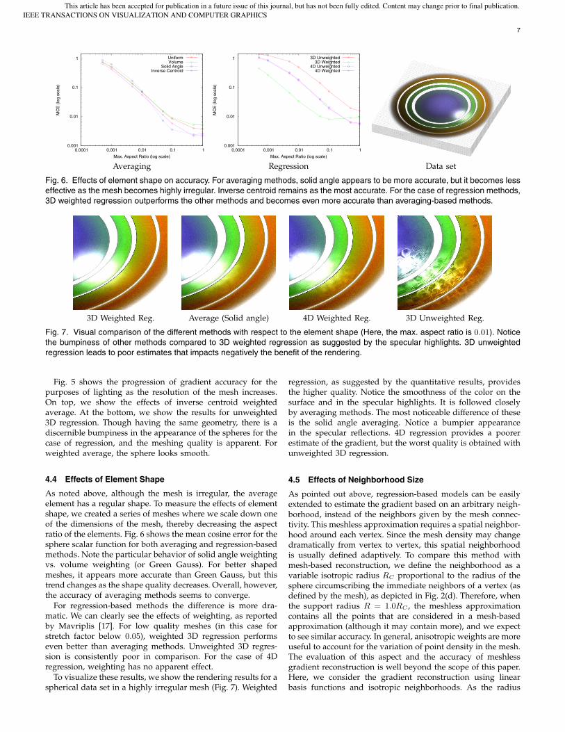
Averaging Regression Data set

Fig. 6. Effects of element shape on accuracy. For averaging methods, solid angle appears to be more accurate, but it becomes lesseffective as the mesh becomes highly irregular. Inverse centroid remains as the most accurate. For the case of regression methods,3D weighted regression outperforms the other methods and becomes even more accurate than averaging-based methods.

3D Weighted Reg. Average (Solid angle) 4D Weighted Reg. 3D Unweighted Reg.

Fig. 7. Visual comparison of the different methods with respect to the element shape (Here, the max. aspect ratio is 0.01). Noticethe bumpiness of other methods compared to 3D weighted regression as suggested by the specular highlights. 3D unweightedregression leads to poor estimates that impacts negatively the benefit of the rendering.

Fig. 5 shows the progression of gradient accuracy for thepurposes of lighting as the resolution of the mesh increases.On top, we show the effects of inverse centroid weightedaverage. At the bottom, we show the results for unweighted3D regression. Though having the same geometry, there is adiscernible bumpiness in the appearance of the spheres for thecase of regression, and the meshing quality is apparent. Forweighted average, the sphere looks smooth.

4.4 Effects of Element Shape

As noted above, although the mesh is irregular, the averageelement has a regular shape. To measure the effects of elementshape, we created a series of meshes where we scale down oneof the dimensions of the mesh, thereby decreasing the aspectratio of the elements. Fig. 6 shows the mean cosine error for thesphere scalar function for both averaging and regression-basedmethods. Note the particular behavior of solid angle weightingvs. volume weighting (or Green Gauss). For better shapedmeshes, it appears more accurate than Green Gauss, but thistrend changes as the shape quality decreases. Overall, however,the accuracy of averaging methods seems to converge.

For regression-based methods the difference is more dra-matic. We can clearly see the effects of weighting, as reportedby Mavriplis [17]. For low quality meshes (in this case forstretch factor below 0.05), weighted 3D regression performseven better than averaging methods. Unweighted 3D regres-sion is consistently poor in comparison. For the case of 4Dregression, weighting has no apparent effect.

To visualize these results, we show the rendering results for aspherical data set in a highly irregular mesh (Fig. 7). Weighted

regression, as suggested by the quantitative results, providesthe higher quality. Notice the smoothness of the color on thesurface and in the specular highlights. It is followed closelyby averaging methods. The most noticeable difference of theseis the solid angle averaging. Notice a bumpier appearancein the specular reflections. 4D regression provides a poorerestimate of the gradient, but the worst quality is obtained withunweighted 3D regression.

4.5 Effects of Neighborhood Size

As pointed out above, regression-based models can be easilyextended to estimate the gradient based on an arbitrary neigh-borhood, instead of the neighbors given by the mesh connec-tivity. This meshless approximation requires a spatial neighbor-hood around each vertex. Since the mesh density may changedramatically from vertex to vertex, this spatial neighborhoodis usually defined adaptively. To compare this method withmesh-based reconstruction, we define the neighborhood as avariable isotropic radius RC proportional to the radius of thesphere circumscribing the immediate neighbors of a vertex (asdefined by the mesh), as depicted in Fig. 2(d). Therefore, whenthe support radius R = 1.0RC , the meshless approximationcontains all the points that are considered in a mesh-basedapproximation (although it may contain more), and we expectto see similar accuracy. In general, anisotropic weights are moreuseful to account for the variation of point density in the mesh.The evaluation of this aspect and the accuracy of meshlessgradient reconstruction is well beyond the scope of this paper.Here, we consider the gradient reconstruction using linearbasis functions and isotropic neighborhoods. As the radius


8

0.001

0.01

0.1

1

0.6 0.8 1 1.2 1.4 1.6 1.8 2 2.2 2.4 2.6

MC

E (

log

scal

e)

Support

Averaging (IC)3D Weighted Regression

MeshlessMeshless (analytic)

0.1

1

0.6 0.8 1 1.2 1.4 1.6 1.8 2 2.2 2.4

MC

E (

log

scal

e)

Support

Averaging (IC)3D Weighted Regression

MeshlessMeshless (analytic)

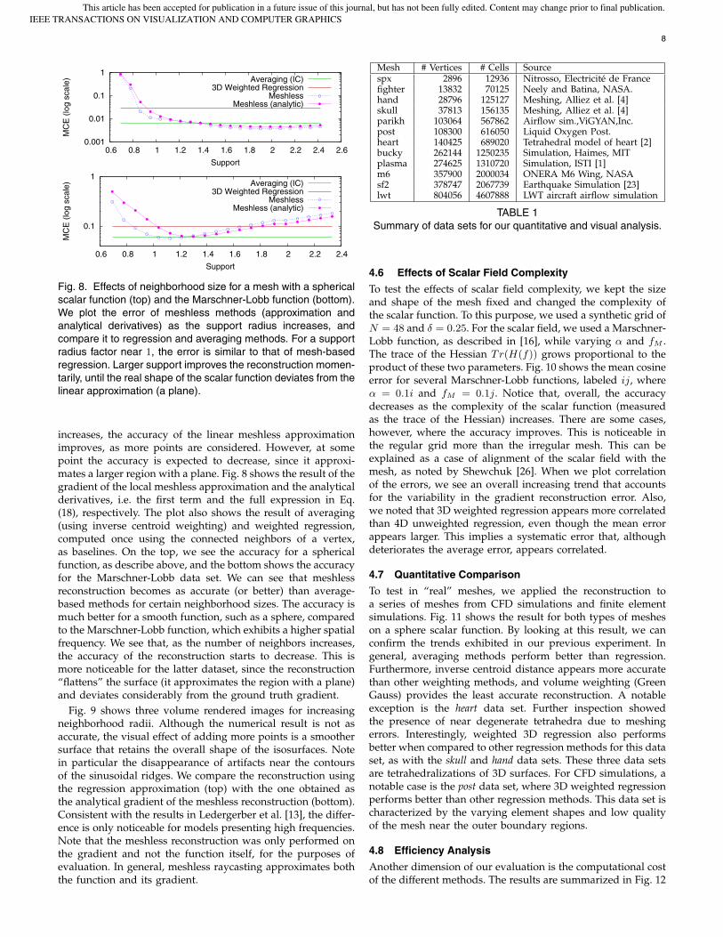
Fig. 8. Effects of neighborhood size for a mesh with a sphericalscalar function (top) and the Marschner-Lobb function (bottom).We plot the error of meshless methods (approximation andanalytical derivatives) as the support radius increases, andcompare it to regression and averaging methods. For a supportradius factor near 1, the error is similar to that of mesh-basedregression. Larger support improves the reconstruction momen-tarily, until the real shape of the scalar function deviates from thelinear approximation (a plane).

increases, the accuracy of the linear meshless approximationimproves, as more points are considered. However, at somepoint the accuracy is expected to decrease, since it approxi-mates a larger region with a plane. Fig. 8 shows the result of thegradient of the local meshless approximation and the analyticalderivatives, i.e. the first term and the full expression in Eq.(18), respectively. The plot also shows the result of averaging(using inverse centroid weighting) and weighted regression,computed once using the connected neighbors of a vertex,as baselines. On the top, we see the accuracy for a sphericalfunction, as describe above, and the bottom shows the accuracyfor the Marschner-Lobb data set. We can see that meshlessreconstruction becomes as accurate (or better) than average-based methods for certain neighborhood sizes. The accuracy ismuch better for a smooth function, such as a sphere, comparedto the Marschner-Lobb function, which exhibits a higher spatialfrequency. We see that, as the number of neighbors increases,the accuracy of the reconstruction starts to decrease. This ismore noticeable for the latter dataset, since the reconstruction“flattens” the surface (it approximates the region with a plane)and deviates considerably from the ground truth gradient.

Fig. 9 shows three volume rendered images for increasingneighborhood radii. Although the numerical result is not asaccurate, the visual effect of adding more points is a smoothersurface that retains the overall shape of the isosurfaces. Notein particular the disappearance of artifacts near the contoursof the sinusoidal ridges. We compare the reconstruction usingthe regression approximation (top) with the one obtained asthe analytical gradient of the meshless reconstruction (bottom).Consistent with the results in Ledergerber et al. [13], the differ-ence is only noticeable for models presenting high frequencies.Note that the meshless reconstruction was only performed onthe gradient and not the function itself, for the purposes ofevaluation. In general, meshless raycasting approximates boththe function and its gradient.

Mesh # Vertices # Cells Sourcespx 2896 12936 Nitrosso, Electricite de Francefighter 13832 70125 Neely and Batina, NASA.hand 28796 125127 Meshing, Alliez et al. [4]skull 37813 156135 Meshing, Alliez et al. [4]parikh 103064 567862 Airflow sim.,ViGYAN,Inc.post 108300 616050 Liquid Oxygen Post.heart 140425 689020 Tetrahedral model of heart [2]bucky 262144 1250235 Simulation, Haimes, MITplasma 274625 1310720 Simulation, ISTI [1]m6 357900 2000034 ONERA M6 Wing, NASAsf2 378747 2067739 Earthquake Simulation [23]lwt 804056 4607888 LWT aircraft airflow simulation

TABLE 1Summary of data sets for our quantitative and visual analysis.

4.6 Effects of Scalar Field Complexity

To test the effects of scalar field complexity, we kept the sizeand shape of the mesh fixed and changed the complexity ofthe scalar function. To this purpose, we used a synthetic grid ofN = 48 and δ = 0.25. For the scalar field, we used a Marschner-Lobb function, as described in [16], while varying α and fM .The trace of the Hessian Tr(H(f)) grows proportional to theproduct of these two parameters. Fig. 10 shows the mean cosineerror for several Marschner-Lobb functions, labeled ij, whereα = 0.1i and fM = 0.1j. Notice that, overall, the accuracydecreases as the complexity of the scalar function (measuredas the trace of the Hessian) increases. There are some cases,however, where the accuracy improves. This is noticeable inthe regular grid more than the irregular mesh. This can beexplained as a case of alignment of the scalar field with themesh, as noted by Shewchuk [26]. When we plot correlationof the errors, we see an overall increasing trend that accountsfor the variability in the gradient reconstruction error. Also,we noted that 3D weighted regression appears more correlatedthan 4D unweighted regression, even though the mean errorappears larger. This implies a systematic error that, althoughdeteriorates the average error, appears correlated.

4.7 Quantitative Comparison

To test in “real” meshes, we applied the reconstruction toa series of meshes from CFD simulations and finite elementsimulations. Fig. 11 shows the result for both types of mesheson a sphere scalar function. By looking at this result, we canconfirm the trends exhibited in our previous experiment. Ingeneral, averaging methods perform better than regression.Furthermore, inverse centroid distance appears more accuratethan other weighting methods, and volume weighting (GreenGauss) provides the least accurate reconstruction. A notableexception is the heart data set. Further inspection showedthe presence of near degenerate tetrahedra due to meshingerrors. Interestingly, weighted 3D regression also performsbetter when compared to other regression methods for this dataset, as with the skull and hand data sets. These three data setsare tetrahedralizations of 3D surfaces. For CFD simulations, anotable case is the post data set, where 3D weighted regressionperforms better than other regression methods. This data set ischaracterized by the varying element shapes and low qualityof the mesh near the outer boundary regions.

4.8 Efficiency Analysis

Another dimension of our evaluation is the computational costof the different methods. The results are summarized in Fig. 12


9

support 1.2 support 1.8 support 2.5

Fig. 9. Visual comparison on the effects of neighborhood size for the Marschner-Lobb scalar function. As we introduce more points,the rendered surfaces become smoother and artifacts due to meshing become less apparent. Increasing the neighborhood furthermakes the surface to appear flatter. Top: Local meshless approximation. Bottom: Analytical derivatives of meshless reconstruction.

0

0.05

0.1

0.15

0.2

0.25

11 21 31 41 12 22 32 42 13 23 33 43 14 24 34 44

MC

E

Dataset

UniformVolume


0 0.005 0.01

0.015 0.02

0.025 0.03

0.035 0.04

0.045

11 21 31 41 12 22 32 42 13 23 33 43 14 24 34 44

Cor

rela

tion

Dataset

UniformVolume


0

0.05

0.1

0.15

0.2

0.25

11 21 31 41 12 22 32 42 13 23 33 43 14 24 34 44

MC

E

Dataset



0 0.005 0.01

0.015 0.02

0.025 0.03

0.035 0.04

0.045

11 21 31 41 12 22 32 42 13 23 33 43 14 24 34 44

Cor

rela

tion

Dataset



Averaging-based methods Regression-based methods

Fig. 10. Effects of scalar field complexity. Averaging-based methods are in general more accurate. Of the regression-basedmethods, 4D weighted is the only comparable, which estimates similar to volume weighting. When these methods are compared interms of correlation, we notice that 3D weighted regression has a better estimate (correlated error) than 4D unweighted regression.3D unweighted regression is significantly less accurate.

0.0001

0.001

0.01

0.1

heart fighter post m6 lwt spx parikh skull hand sf2 plasma bucky

MC

E

Mesh

UniformVolume

Solid Angle Inverse Centroid

0.0001

0.001

0.01

0.1

heart fighter post m6 lwt spx parikh skull hand sf2 plasma bucky

MC

E

Mesh

3D unweighted3D Weighted

4D unweighted4D Weighted

Averaging-based methods Regression-based meshes

Fig. 11. Comparison of gradient reconstructions for different meshes with an embedded spherical scalar field.


10

0

0.1

0.2

0.3

0.4

0.5

0.6

0.7

0.8

0.9

1

8 16 24 32 40 48 56 64 72 80 88

Tim

e (s

econ

ds)

Size

Green Gauss

3D Unweighted3D Weighted, Uniform4D Unweighted4D WeightedVolume

Inverse CentroidSolid Angle

Fig. 12. Time to compute gradient for test benchmark (gridwith δ = 0.25, sphere scalar field). The Green Gauss methodis significantly faster than the rest (including volume-weightedaveraging, which produces equivalent results). Weighting maybe costly for averaging methods, but does not have a significantimpact in regression-based methods.

for the synthetic data sets. We used an Intel Core 2 quad-coreprocessor with 3.0 GHz and 4GB of RAM. The results wereobtained in a CPU-based implementation using a comparableset of operations for each of the methods. We expect the relativeperformance of each method to be similar under different ma-chines, including GPUs. Although parallel computation maydecrease the gap between the different methods, the relativecost per element is still the same. Cell average is in generalthe costliest approach, in particular for the solid angle andinverse centroid weighting schemes. Green Gauss, on the otherhand, is the fastest of all methods. Compare it to averagingwith volume weighting, which provides equivalent results.Regression methods do not differ greatly in speed, and thecost of weighting is insignificant in comparison to unweightedregression, and are out-weighted by their benefits in accuracy.Due to the speed, Green Gauss reconstruction is attractivefor interactive visualization. However, as seen above, volumeweighted reconstruction is not robust to low quality meshes,whereas 3D weighted regression is. This motivates one of ourheuristic methods, which combines the benefits of these twoapproaches, as described in Section 5.1.

4.9 Visual Comparison

Fig. 13 shows the volume rendering of a jet wing wind simula-tion data set. This is a representative mesh of CFD simulations,where an adaptive mesh is used to populate densely regionsof interest (around the wing and missile). In our rendering,we aim at highlighting the shock waves on the wing. Lightinghelps understand the shape of these shock waves. As suggestedby the quantitative results, all methods produce good results onhigh-quality regions, while differences become noticeable forpoor quality tetrahedra. As we move from averaging methodsto 3D regression, we see a decrease in quality. At the bottomof Fig. 13, we provide close-up views of certain regions of thevolume and compare the results for inverse centroid weightedaverage and unweighted 3D regression. On the left, we see theeffects of meshing more noticeable in the case of 3D regressionas shown in the shape of the specular highlight. In the middle,weighted average shows a smoother surface near the boundary

of the mesh. On the right, a portion of one of the shock wavesappears smooth when using averaging, but appears brokenand bumpy for the case of 3D regression.

Fig. 14 shows a different case, where a smoothly changingfunction is embedded in a variable quality mesh (oxygen postdata set). Both weighted regression and cell average methodsproduce similar results. The Green-Gauss method is also sim-ilar, except for a few changes in the apparent curvature of theshapes due to the use of low quality cells near the boundary.Unweighted regression suffers most from the low quality of themesh. In this case, poor quality gradient reconstruction leadsto the appearance of creases and folds where there are none,and the apparent flatness of regions where there should be asmooth curved surface.

5 IMPLICATIONS

Our study has provided interesting insight on the behavior ofdifferent gradient reconstruction methods for the purposes oflighting. We summarize these as follows:

(1) Averaging-based methods provide the most accurategradient reconstruction in general, and the inverse centroiddistance is consistently more accurate than other methods, suchas Green Gauss, that are based on volume weighting. This isespecially true for highly regular meshes.

(2) Regression-based methods are less accurate, but canadapt better to low quality meshes. Unweighted regressionleads to poor gradient reconstructions, especially when themesh is highly irregular. Since inverse distance weighted re-gression has a similar computational cost, it should be pre-ferred. The benefits of this weighting, however, do not applyfor 4D regression, which behaves similar to volume weightedaveraging.

(3) To improve the accuracy of the reconstruction, one mayhave to increase the neighborhood. Although this would re-quire an additional structure for weighted cell average meth-ods, as it requires to find the extended cell neighborhood ofa cell, it becomes easy to do for regression-based methods.Inverse distance weighting leads to a Moving Least Squaresreconstruction, popular in surface reconstruction from pointsets. Although introducing more points produces smoother re-sults, they are not necessarily more accurate, as it approximatesregions with high frequencies to planes.

(4) Although volume weighted average and Green-Gaussare equivalent, their implementations differ greatly and thespeed gap becomes noticeable. The Green-Gauss method thenbecomes attractive for interactive rendering systems.

Based on our observations we propose two heuristics forobtaining high-quality rendering of unstructured meshes atreasonable speeds.

5.1 Hybrid Gradient Reconstruction

Similar to recent hybrid rendering methods, we can derive ahybrid gradient reconstruction method that favors a methoddepending on the local structure of the mesh. Many unstruc-tured meshes, particularly in CFD simulations, are definedadaptively, so that large tetrahedra are located in regions of lowinterest, whereas small tetrahedra populate regions of interest.Connecting these usually results in tetrahedra of disparatesize and aspect ratios. By probing the mesh quality in a pre-processing step, we can define the gradient using averagingmethods for high quality regions and regression for low qualityregions.


11

Avg. Volume Avg. Inverse Centroid (IC) 3D Weighted Regression 3D Unweighted Regression

Avg (IC). 3D U.Reg Avg (IC). 3D U.Reg Avg (IC). 3D U.Reg

Fig. 13. Visual comparison of four methods for a aerodynamics flow simulation. Here, lighting helps understand the shape of theshock waves around the wing of an aircraft. At the bottom, close up views of different regions show that gradients in unweightedregression make the meshing evident, while surfaces appear smoother with averaging.

Weighted Reg. Average (Inv. centroid) Green-Gauss Unweighted Reg.

Fig. 14. Visual comparison of a smoothly changing function on a variable quality mesh (Oxygen post data set). Regions of goodmesh quality (near the post) are reconstructed well for all methods. Because the function is smoothly changing, there is littledifference between regression and averaging methods. For the Green Gauss methods, the shape appears more pronounced nearthe boundary (where there are poor quality cells). For unweighted regression, the effects of a poor quality mesh are more dramatic.Some regions appear to have creases and folds where there are none, while some other regions appear flat.

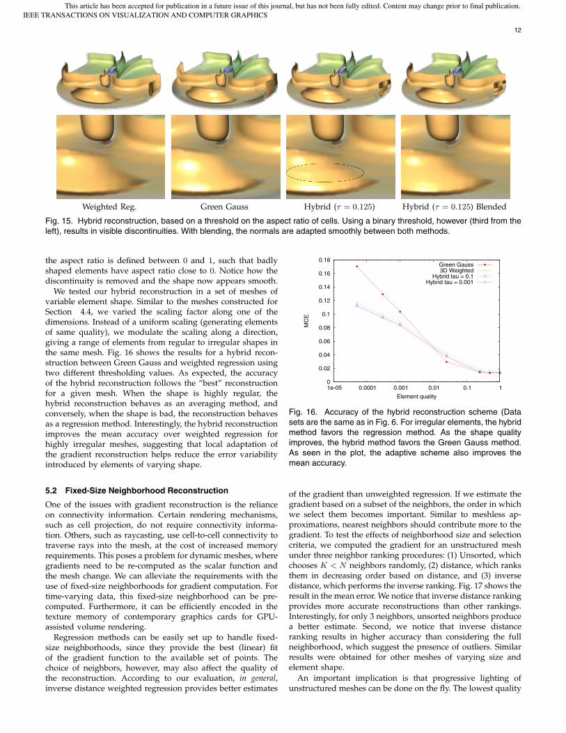
For example, Fig. 15 shows the results of applying hy-brid gradient reconstruction to the oxygen post data set. Wesee a difference between the shape of features as estimatedby the weighted regression and Green Gauss methods, assuggested by the specular highlights. Green Gauss methodsalso introduce mesh-aligned normals near the boundaries, butthe normals are, for the most part, smoother. The hybridreconstruction uses a threshold τ = 0.125 on the aspectratio to determine which method to use. Regression is onlyused when the minimum aspect ratio of the neighboring cellsof a vertex is less than τ . This binary operator introducesdiscontinuities, as shown in the third image from the left.To avoid artifacts in the boundary of these two regions, wedefine a continuous measure, clamped between 0 and 1, anduse it as a modulation factor in linear (or spherical) blendingbetween the two normals. Let us define nG(x) and nW (x)

as the gradients computed using Green-Gauss and weightedregression, respectively. The normal at a given point can befound as:

n(x) = α(x)nG(x) + (1− α(x))nw(x) (20)

where α(x) ∈ [0, 1] is a function of volume, aspect ratio or anyother metric that describes the irregularity of the mesh at anygiven point. To avoid computing two normals for each point,this equation only needs to compute one of them when α(x)tends to 0 or 1. In Fig. 15, we use:

α(x) =

»mini∈Neigh(x)(A(i)− τ)

τ

–1

0

(21)

where A(i) is the aspect ratio of element i, Neigh(x) is the setof incident cells of vertex x, and [x]10 is a clamping operationthat keeps the values between 0 and 1. Here, we assume that


12

Weighted Reg. Green Gauss Hybrid (τ = 0.125) Hybrid (τ = 0.125) Blended

Fig. 15. Hybrid reconstruction, based on a threshold on the aspect ratio of cells. Using a binary threshold, however (third from theleft), results in visible discontinuities. With blending, the normals are adapted smoothly between both methods.

the aspect ratio is defined between 0 and 1, such that badlyshaped elements have aspect ratio close to 0. Notice how thediscontinuity is removed and the shape now appears smooth.

We tested our hybrid reconstruction in a set of meshes ofvariable element shape. Similar to the meshes constructed forSection 4.4, we varied the scaling factor along one of thedimensions. Instead of a uniform scaling (generating elementsof same quality), we modulate the scaling along a direction,giving a range of elements from regular to irregular shapes inthe same mesh. Fig. 16 shows the results for a hybrid recon-struction between Green Gauss and weighted regression usingtwo different thresholding values. As expected, the accuracyof the hybrid reconstruction follows the “best” reconstructionfor a given mesh. When the shape is highly regular, thehybrid reconstruction behaves as an averaging method, andconversely, when the shape is bad, the reconstruction behavesas a regression method. Interestingly, the hybrid reconstructionimproves the mean accuracy over weighted regression forhighly irregular meshes, suggesting that local adaptation ofthe gradient reconstruction helps reduce the error variabilityintroduced by elements of varying shape.

5.2 Fixed-Size Neighborhood Reconstruction

One of the issues with gradient reconstruction is the relianceon connectivity information. Certain rendering mechanisms,such as cell projection, do not require connectivity informa-tion. Others, such as raycasting, use cell-to-cell connectivity totraverse rays into the mesh, at the cost of increased memoryrequirements. This poses a problem for dynamic meshes, wheregradients need to be re-computed as the scalar function andthe mesh change. We can alleviate the requirements with theuse of fixed-size neighborhoods for gradient computation. Fortime-varying data, this fixed-size neighborhood can be pre-computed. Furthermore, it can be efficiently encoded in thetexture memory of contemporary graphics cards for GPU-assisted volume rendering.

Regression methods can be easily set up to handle fixed-size neighborhoods, since they provide the best (linear) fitof the gradient function to the available set of points. Thechoice of neighbors, however, may also affect the quality ofthe reconstruction. According to our evaluation, in general,inverse distance weighted regression provides better estimates

0

0.02

0.04

0.06

0.08

0.1

0.12

0.14

0.16

0.18

1e-05 0.0001 0.001 0.01 0.1 1

MC

E

Element quality

Green Gauss3D Weighted

Hybrid tau = 0.1Hybrid tau = 0.001

Fig. 16. Accuracy of the hybrid reconstruction scheme (Datasets are the same as in Fig. 6. For irregular elements, the hybridmethod favors the regression method. As the shape qualityimproves, the hybrid method favors the Green Gauss method.As seen in the plot, the adaptive scheme also improves themean accuracy.

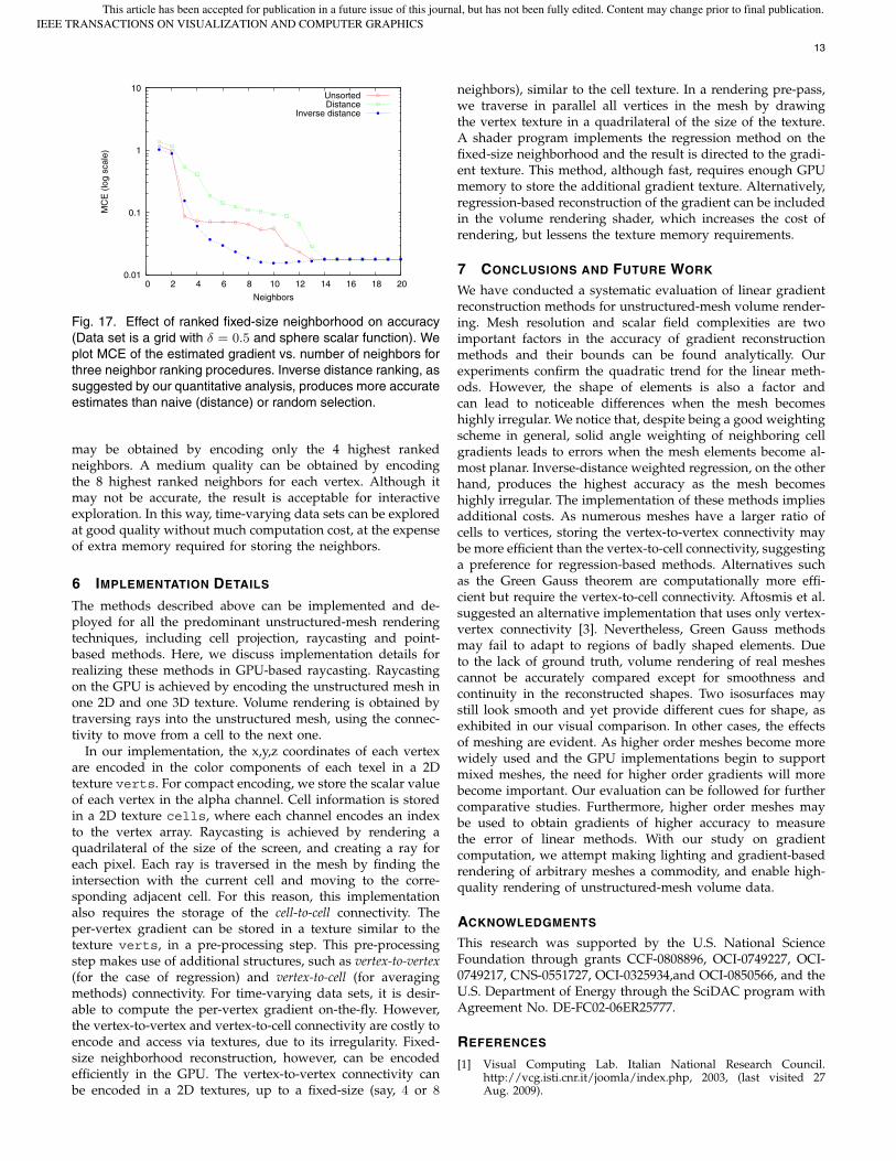
of the gradient than unweighted regression. If we estimate thegradient based on a subset of the neighbors, the order in whichwe select them becomes important. Similar to meshless ap-proximations, nearest neighbors should contribute more to thegradient. To test the effects of neighborhood size and selectioncriteria, we computed the gradient for an unstructured meshunder three neighbor ranking procedures: (1) Unsorted, whichchooses K < N neighbors randomly, (2) distance, which ranksthem in decreasing order based on distance, and (3) inversedistance, which performs the inverse ranking. Fig. 17 shows theresult in the mean error. We notice that inverse distance rankingprovides more accurate reconstructions than other rankings.Interestingly, for only 3 neighbors, unsorted neighbors producea better estimate. Second, we notice that inverse distanceranking results in higher accuracy than considering the fullneighborhood, which suggest the presence of outliers. Similarresults were obtained for other meshes of varying size andelement shape.

An important implication is that progressive lighting ofunstructured meshes can be done on the fly. The lowest quality


13

0.01

0.1

1

10

0 2 4 6 8 10 12 14 16 18 20

MC

E (

log

scal

e)

Neighbors

UnsortedDistance

Inverse distance

Fig. 17. Effect of ranked fixed-size neighborhood on accuracy(Data set is a grid with δ = 0.5 and sphere scalar function). Weplot MCE of the estimated gradient vs. number of neighbors forthree neighbor ranking procedures. Inverse distance ranking, assuggested by our quantitative analysis, produces more accurateestimates than naive (distance) or random selection.

may be obtained by encoding only the 4 highest rankedneighbors. A medium quality can be obtained by encodingthe 8 highest ranked neighbors for each vertex. Although itmay not be accurate, the result is acceptable for interactiveexploration. In this way, time-varying data sets can be exploredat good quality without much computation cost, at the expenseof extra memory required for storing the neighbors.

6 IMPLEMENTATION DETAILS

The methods described above can be implemented and de-ployed for all the predominant unstructured-mesh renderingtechniques, including cell projection, raycasting and point-based methods. Here, we discuss implementation details forrealizing these methods in GPU-based raycasting. Raycastingon the GPU is achieved by encoding the unstructured mesh inone 2D and one 3D texture. Volume rendering is obtained bytraversing rays into the unstructured mesh, using the connec-tivity to move from a cell to the next one.

In our implementation, the x,y,z coordinates of each vertexare encoded in the color components of each texel in a 2Dtexture verts. For compact encoding, we store the scalar valueof each vertex in the alpha channel. Cell information is storedin a 2D texture cells, where each channel encodes an indexto the vertex array. Raycasting is achieved by rendering aquadrilateral of the size of the screen, and creating a ray foreach pixel. Each ray is traversed in the mesh by finding theintersection with the current cell and moving to the corre-sponding adjacent cell. For this reason, this implementationalso requires the storage of the cell-to-cell connectivity. Theper-vertex gradient can be stored in a texture similar to thetexture verts, in a pre-processing step. This pre-processingstep makes use of additional structures, such as vertex-to-vertex(for the case of regression) and vertex-to-cell (for averagingmethods) connectivity. For time-varying data sets, it is desir-able to compute the per-vertex gradient on-the-fly. However,the vertex-to-vertex and vertex-to-cell connectivity are costly toencode and access via textures, due to its irregularity. Fixed-size neighborhood reconstruction, however, can be encodedefficiently in the GPU. The vertex-to-vertex connectivity canbe encoded in a 2D textures, up to a fixed-size (say, 4 or 8

neighbors), similar to the cell texture. In a rendering pre-pass,we traverse in parallel all vertices in the mesh by drawingthe vertex texture in a quadrilateral of the size of the texture.A shader program implements the regression method on thefixed-size neighborhood and the result is directed to the gradi-ent texture. This method, although fast, requires enough GPUmemory to store the additional gradient texture. Alternatively,regression-based reconstruction of the gradient can be includedin the volume rendering shader, which increases the cost ofrendering, but lessens the texture memory requirements.

7 CONCLUSIONS AND FUTURE WORK

We have conducted a systematic evaluation of linear gradientreconstruction methods for unstructured-mesh volume render-ing. Mesh resolution and scalar field complexities are twoimportant factors in the accuracy of gradient reconstructionmethods and their bounds can be found analytically. Ourexperiments confirm the quadratic trend for the linear meth-ods. However, the shape of elements is also a factor andcan lead to noticeable differences when the mesh becomeshighly irregular. We notice that, despite being a good weightingscheme in general, solid angle weighting of neighboring cellgradients leads to errors when the mesh elements become al-most planar. Inverse-distance weighted regression, on the otherhand, produces the highest accuracy as the mesh becomeshighly irregular. The implementation of these methods impliesadditional costs. As numerous meshes have a larger ratio ofcells to vertices, storing the vertex-to-vertex connectivity maybe more efficient than the vertex-to-cell connectivity, suggestinga preference for regression-based methods. Alternatives suchas the Green Gauss theorem are computationally more effi-cient but require the vertex-to-cell connectivity. Aftosmis et al.suggested an alternative implementation that uses only vertex-vertex connectivity [3]. Nevertheless, Green Gauss methodsmay fail to adapt to regions of badly shaped elements. Dueto the lack of ground truth, volume rendering of real meshescannot be accurately compared except for smoothness andcontinuity in the reconstructed shapes. Two isosurfaces maystill look smooth and yet provide different cues for shape, asexhibited in our visual comparison. In other cases, the effectsof meshing are evident. As higher order meshes become morewidely used and the GPU implementations begin to supportmixed meshes, the need for higher order gradients will morebecome important. Our evaluation can be followed for furthercomparative studies. Furthermore, higher order meshes maybe used to obtain gradients of higher accuracy to measurethe error of linear methods. With our study on gradientcomputation, we attempt making lighting and gradient-basedrendering of arbitrary meshes a commodity, and enable high-quality rendering of unstructured-mesh volume data.

ACKNOWLEDGMENTS

This research was supported by the U.S. National ScienceFoundation through grants CCF-0808896, OCI-0749227, OCI-0749217, CNS-0551727, OCI-0325934,and OCI-0850566, and theU.S. Department of Energy through the SciDAC program withAgreement No. DE-FC02-06ER25777.

REFERENCES

[1] Visual Computing Lab. Italian National Research Council.http://vcg.isti.cnr.it/joomla/index.php, 2003, (last visited 27Aug. 2009).


14

[2] Computational Visualization Center, University of Texasat Austin. Tetrahedral model of the human heart.http://cvcweb.ices.utexas.edu/cvc/, 2008 (last visited 27 Aug.2009).

[3] M. Aftosmis, D. Gaitonde, and T. Tavares. Behavior of linearreconstruction techniques on unstructured meshes. AIAA Journal,33(11):2038–2049, 1995.

[4] P. Alliez, D. Cohen-Steiner, M. Yvinec, and M. Desbrun. Vari-ational tetrahedral meshing. ACM Trans. Graph., 24(3):617–625,2005.

[5] W. K. Anderson and D. L. Bonhaus. An implicit upwind algorithmfor computing turbulent flows on unstructured grids. Comput.Fluids, 23(1):1–21, 1994.

[6] T. Apel, M. Berzins, P. Jimack, G. Kunert, A. Plaks, I. Tsukerman,and M.Walkley. Mesh shape and anisotropic elements: theoryand practice. In The Tenth Conference on The Mathematics of FiniteElements and Applications, pages 367–376, 1999.

[7] T. J. Barth and D. C. Jerspesen. The design and application ofupwind schemes on unstructured meshes. In Proc. 27th AerospaceSciences Meeting. Paper AIAA 89-0366, 1989.

[8] M. J. Bentum, B. B. A. Lichtenbelt, and T. Malzbender. Frequencyanalysis of gradient estimators in volume rendering. IEEE Trans.on Visualization and Computer Graphics, 2(3):242–254, 1996.

[9] S. P. Callahan, J. L. D. Comba, M. Ikits, and M.-C. T. Silva.Hardware-assisted visibility sorting for unstructured volume ren-dering. IEEE Trans. on Visualization and Computer Graphics,11(3):285–295, 2005.

[10] P. Cignoni, C. Montani, and R. Scopigno. Tetrahedra basedvolume visualization. Mathematical Visualization, pages 3–18, 1998.

[11] M. P. Garrity. Raytracing irregular volume data. In VVS ’90: Proc.of the 1990 workshop on Volume visualization, pages 35–40, 1990.

[12] H. Hoppe, T. DeRose, T. Duchamp, J. McDonald, and W. Stuetzle.Surface reconstruction from unorganized points. In SIGGRAPH’92: Proc. of the 19th annual conference on Computer graphics andinteractive techniques, pages 71–78, 1992.

[13] C. Ledergerber, G. Guennebaud, M. Meyer, M. Bacher, and H. Pfis-ter. Volume MLS ray casting. IEEE Trans. on Visualization andComputer Graphics, 14(6):1539–1546, 2008.

[14] B. Levy, G. Caumon, S. Conreaux, and X. Cavin. Circular incidentedge lists: a data structure for rendering complex unstructuredgrids. In Proc. IEEE Visualization ’01, pages 191–198, 2001.

[15] K.-L. Ma, J. V. Rosendale, and W. Vermeer. 3d shock wavevisualization on unstructured grids. In Proc. of the 1996 symposiumon Volume visualization, pages 87–94., 1996.

[16] S. R. Marschner and R. J. Lobb. An evaluation of reconstructionfilters for volume rendering. In Proc. IEEE Visualization ’94, pages100–107, 1994.

[17] J. Mavriplis. Revisiting the least-squares procedure for gradientreconstruction on unstructured meshes. In Proc. AIAA Computa-tional Fluid Dynamics Conference. Paper AIAA 2003-3986, 2003.

[18] J. Meredith and K.-L. Ma. Multiresolution view-dependent splatbased volume rendering of large irregular data. In Proc. IEEESymp. on parallel and large-data visualization and graphics, pages 93–99, 2001.

[19] T. H. Meyer, M. Eriksson, and R. C. Maggio. Gradient estimationfrom irregularly spaced data sets. Mathematical Geology, 33(6):693–717, 2001.

[20] T. Moller, R. Machiraju, K. Mueller, and R. Yagel. A comparisonof normal estimation schemes. In Proc. IEEE Visualization 1997,pages 19–26., 1997.

[21] P. Muigg, M. Hadwiger, H. Doleisch, and H. Hauser. Scalablehybrid unstructured and structured grid raycasting. IEEE Trans.on Visualization and Computer Graphics, 13(6):1592–1599, Nov.-Dec.2007.

[22] L. Neumann, B. Csebfalvi, A. Konig, and E. Groller. Gradientestimation in volume data using 4D linear regression. In ComputerGraphics Forum, volume 19(3), pages 351–358, 2000.

[23] D. R. O’Hallaron and J. R. Shewchuk. Properties of a familyof parallel finite element simulations. Technical report, CarnegieMellon, 1996.

[24] M. Pauly, R. Keiser, L. P. Kobbelt, and M. Gross. Shape modelingwith point-sampled geometry. ACM Trans.Graph., 22(3):641–650,2003.

[25] N. B. Petrovskaya. The impact of grid cell geometry on theleast-squares gradient reconstruction. Technical report, KeldyshInstitute of Applied Mathematics, Russian Academy of Sciences,2003.

[26] J. R. Shewchuk. What is a good linear finite element? interpo-lation, conditioning, anisotropy, and quality measures. page 66,2002.

[27] P. Shirley and A. Tuchman. A polygonal approximation to directscalar volume rendering. SIGGRAPH Comput. Graph., 24(5):63–70,1990.

[28] G. Thurmer and C. A. Wuthrich. Normal computation for discretesurfaces in 3D space. Comput. Graph. Forum, 16(3):15–26, 1997.

[29] M. Weiler and T. Ertl. Hardware-software-balanced resamplingfor the interactive visualization of unstructured grids. In Proc.IEEE Visualization 2001, pages 199–206, 2001.

[30] M. Weiler, M. Kraus, M. Merz, and T. Ertl. Hardware-based raycasting for tetrahedral meshes. In Proc. IEEE Visualization 2003,pages 333–340, 2003.

[31] R. Westermann. The rendering of unstructured grids revisited. InProc. of the 3rd Joint IEEE TVCG-EUROGRAPHICS Symposium onVisualization (VisSym 2001), pages 65–74, 2001.

[32] L. Westover. Footprint evaluation for volume rendering. InSIGGRAPH ’90: Proc. of the 17th conference on Computer graphicsand interactive techniques, pages 367–376, 1990.

[33] R. Yagel, D. Cohen, and A. Kaufman. Normal estimation in 3Ddiscrete space. The Visual Computer, 8(5-6):278–291, 1992.

[34] Y. Zhou and M. Garland. Interactive point-based rendering ofhigher-order tetrahedral data. IEEE Trans. on Visualization andComputer Graphics, 12(5):1229–1236, 2006.

Carlos D. Correa received the BS degreein computer science from EAFIT University,Colombia, in 1998, and the MS and PhD de-grees in electrical and computer engineeringfrom Rutgers University in 2003 and 2007, re-spectively. Currently, he is a postdoctoral re-searcher in the Department of Computer Sci-ence, University of California, Davis. His re-search interests include computer graphics, vi-sualization and user interaction.

Robert Hero is a PhD student in computerscience from the University of California, Davis.He obtained his MS degree in computer sciencefrom the University of California, Santa Cruz. Hisresearch interests include GPU-based comput-ing and visualization.

Kwan-Liu Ma is a professor of computer sci-ence and the chair of the Graduate Group inComputer Science (GGCS) at the University ofCalifornia, Davis. He leads the VIDI researchgroup and directs the DOE SciDAC Institutefor Ultrascale Visualization, which involves re-searchers from three other universities and twoDOE national laboratories. Professor Ma re-ceived his PhD degree in computer science fromthe University of Utah in 1993. His researchinterests include visualization, high-performance

computing and user interface design. He is the paper chair of the IEEEVisualization Conference in 2008 and 2009. He is the founder of theIEEE Pacific Visualization Symposium. Professor Ma also serves on theeditorial boards of the IEEE Computer Graphics and Applications andthe IEEE Transactions on Visualization and Graphics. He is a seniormember of the IEEE.


a comparison of gradient estimation methods for volume

Documents