a comparison of the silent base ow and vortex sound

A comparison of the silent base flow and vortex sound

analogy sources in high speed subsonic jets

S. Sinayoko∗,

Department of Engineering, University of Cambridge

A. Agarwal †

Department of Engineering, University of Cambridge

Definitions of the sound sources obtained by re-arranging the Navier-Stokes equations

are dependent on two choices: the base flow on the one hand, the dependent variables on

the other hand. This paper chooses a silent base flow for the former, and compares two

different options for the latter. The first option, analogous to that chosen by Lighthill,

uses density, momentum and modified pressure as the dependent variables. The second

options, proposed by Doak, uses total enthalpy, velocity and entropy and is related to

vortex sound theory. The resulting silent base flow sources are computed and compared

for two simulated high speed subsonic jets obtained by direct numerical simulation. It

is shown that, despite having different expressions, both formulations identify the same

noise generation mechanism. In particular, the divergence of the source terms are in close

agreement.

Introduction

The best way of defining aeroacoustic sources, in the framework of acoustic analogies, is still being

debated. Each definition is based on two main ingredients: the first is the choice of base flow about which

the flow equations will be linearised, the second the choice of dependent variables.

Several choices, of increasing complexity, have been made for the base flow: a quiescent base flow

(Lighthill1); a parallel base flow (Lilley2); a potential flow (Howe3); a time-averaged base flow (Bailly et

al,4 Golstein5); a silent base flow (Goldstein,6 Sinayoko et al7). Sinayoko et al8 compared three of these

∗Research Associate, Department of Engineering, University of Cambridge†Lecturer, Department of Engineering, University of Cambridge

1 of 17

American Institute of Aeronautics and Astronautics

acoustic analogies, for the simplified Mach 0.9 jet simulated by Suponitsky et al,9 and showed how each

choice of base flow can lead to very different source distributions. They found that the silent base flow,

as predicted by Goldstein,6 was the most helpful in helping to uncover the underlying physical mechanism

(scattering of longitudinal hydrodynamic wavepackets by mean flow gradients in this case). The definition

of the sound sources presented in this paper will therefore be based on a silent base flow.

The second ingredient, the choice of dependent variables, has received less attention. In generalizing

Powell’s low Mach number vortex sound theory10 to high Mach number flows, Howe chose the total enthalpy

(H = h + v2/2) as the main acoustic variable, rather than Lighthill’s density. Doak11 also constructed a

case for choosing total enthalpy by deriving a generalized wave equation for fluctuations of total enthalpy

in a turbulent flow. In the context of the Ffowcs-Williams and Hawkings equations,12 Morfey et al,13 and

Spalart et al14 demonstrated that it was preferable to recast the equations in terms of the pressure field,

rather than the density field.

The form taken by the sound sources in the above studies is worth discussing in more detail. On the

one hand, Howe15 and Doak’s11 theories lead to sound sources that feature the Lamb vector (∇× v)× v as

their main element. On the other hand, the sources obtained1,7 using density as the main acoustic variable

are dominated by the second order tensor v ⊗ v. Interestingly, the dominant source terms identified in

Sinayoko et al’s study8 was the shear noise source vz0(vz − vz0) (product of axial silent mean flow with

axial hydrodynamic fluctuations), which is missing from the Lamb vector since it only involves products of

axial and radial velocities (and their gradients). This suggests that vortex sound theory, despite successful

applications by Ewert and Schroder,16 may be less appropriate for high Mach number flows. To clarify this

issue, one can compare the radiating part of each source term, i.e. the part that satisfies the dispersion

relation k = ω/c∞ in the Fourier domain.8

The main objective of this paper is to investigate the effect of the choice of dependent variables on

the radiating components of the sound source. Two different choices will be compared. The first choice,

analogous to Lighthill’s, makes density, momentum and modified pressure (ρ, ρv, π) the dependent variables.

The second options, proposed by Doak, uses instead total enthalpy, velocity and entropy (H,S,v) and is

related to vortex sound theory. The corresponding sources will be computed for the high subsonic jets of

Suponitsky et al17 (laminar) and Sandberg et al18 (turbulent).

Margnat et al19 conducted a similar study in which they decomposed Lighthill’s source terms into 10

sub-components including the Lamb vector for a mixing layer of Mach 0.25. Although most of the terms

were found to be weak sources of noise, they found that several terms other than the Lamb vector played an

important role in noise generation within Lightill’s source term. On the other hand, Howe20 showed by using

Lighthill’s analogy that for at low Mach number flow embedded in a quiescent medium, the Lamb vector

2 of 17


is the dominant radiating term. The current paper will investigate this issue in the case of high subsonic

jets. The results will be obtained by examining the radiating part of the sound sources, using the radiation

criteria |k| = ω/c∞ and |kz| ≤ ω/c∞.

The structure of the paper is as follows. Part I presents the two different formulations, part II presents

compares the sound sources for the laminar jet, and part III for the turbulent jet. Part III presents the first

validation of the silent base flow sources for a fully turbulent jet.

I. Theory

A. Criterion for identifying the silent base flow

Using q = ρ, ρv, π as the set of dependent variables, each flow variable q can be decomposed as

q = q + q′, (1)

where q denotes the non-radiating part of q and q′ the radiating part. The radiating part corresponds to the

acoustic part of q in the far field. The decomposition is carried out in the frequency–wavenumber domain

by observing that, for each frequency ω, the radiating components q′ lie on the radiating sphere of radius

|k| = ω/c∞ in the wavenumber domain.6,7, 21 Thus, if Q denotes the space-time Fourier transform of q, then

Q(k, ω) = 0 if |k| = |ω|/c∞ (2)

Q(k, ω) = 1 if |k| 6= |ω|/c∞. (3)

B. Silent base flow formulation based on density

We assume an unbounded, homentropic, perfect gas jet flow of a low Reynolds number (< 104 based on jet

diameter and exit velocity), that is surrounded by a quiescent medium.

Although restrictive, these conditions are sufficient to capture the sound generation from large scale struc-

tures in subsonic jets.22 Other effects due, for example, to the presence of solid boundaries,12 temperature

gradients2 or supersonic speeds23 will be ignored for simplicity.

The flow satisfies the following equations:7

∂ρ

∂t+

∂

∂xjρvj = 0, (4)

∂

∂tρvi +

∂

∂xjρvivj +

∂

∂xiπγ = 0, (5)

∂π

∂t+

∂

∂xjπvj = 0. (6)

3 of 17


where ρ denotes the density, v the velocity field, π = p1/γ the modified pressure field, where p is the pressure

field and γ the specific heat ratio.

From,7 the radiating components q′ satisfy an equation of the form

L1(q′) = s1′, (7)

where L1 is a linear operator, s′1 = 0, f ′1, 0 and f ′1 represents the momentum equation source term defined

as

f ′1i = − ∂

∂xj( ρ vivj )

′. (8)

In equation (8), vi = ρvi/ρ denotes Favre averaged velocity. The NRBF source s1 depends only on the

non-radiating flow variables q.

C. Silent base flow formulation based on total enthalpy

For a homentropic flow, based on Doak’s derivation,11 the flow equations can written as

1

c2

(∂H

∂t+ 2vj

∂H

∂xj

)+

∂

∂xi−MiMj

∂

∂xj

vi = 0, (9)

∂vi∂t

+∂H

∂xi= −(Ω× v)i (10)

S = constant (11)

where H = h+ v2/2 denotes the total enthalpy and S the entropy.

The radiating components q′ satisfy an equation of the form

L2(q′) = s2′, (12)

where L2 is a linear operator and s2′ = l′, f ′2, 0, where l′ and f ′2 are defined as

l′ = −(M iM j

∂vi∂xj

)′, f ′2i = −(Ω× v)′i. (13)

(14)

4 of 17


II. Laminar jet results

A. Numerical simulation

We now consider a nonlinear problem in which an axisymmetric jet is excited by two discrete-frequency

axisymmetric disturbances at the jet exit. The frequencies are chosen to trigger some instability waves in

the flow. These instability waves grow downstream and interact non-linearly, generating acoustic waves. The

Mach number of the jet is 0.9 and the Reynolds number is 3600. The base mean flow is chosen to match the

experimental data of Stromberg et al.24

Suponitsky et al25 performed direct numerical simulations of the compressible Navier–Stokes equations

for this problem. In their simulations the mean flow was prescribed by imposing time-independent forcing

terms. They ran simulations with different combinations of excitation frequencies and amplitudes. The

data used here corresponds to the combination with the largest acoustic radiation. The two excitation

frequencies are ω1 = 2.2 and ω2 = 3.4. Sound radiates mainly at the difference frequency ∆ω = 1.2. The

results presented in this section have been normalised by using the jet diameter D, jet exit speed Uj and the

ambient density as the length, velocity and density scales, respectively.

B. Axial sound sources

The non-radiating base flow sources were computed by Sinayoko et al8 using the density-based formulation of

equation (8). We now revisit these results to compare them to the enthalpy-based formulation of equation (8).

We focus on the axial source term at frequency ω = 1.2, which is the dominant source term in this flow.8

From equations (8) and (13), the dominant source term for each formulation reduces to

f ′1z ≈∂

∂z(ρ vz vz)

′, f ′2z ≈ (Ωvr)′ =

[(∂vz∂r− ∂vr

∂z

)vr

]′. (15)

Since we know from8 that the dominant noise mechanism is related to velocity fluctuations rather than

density fluctuations, we will use the approximation ρ ≈ ρ∞ in the expression of f1z, i.e.

f ′1z/ρ∞ ≈∂

∂z(vz vz)

′, f ′2z ≈[(

∂vz∂r− ∂vr

∂z

)vr

]′. (16)

Finally, the filter can be applied frequency by frequency. The resulting source at frequency ω = 1.2 is given

by

(f1z)′1.2 ≈

∂

∂z(vz vz)

′1.2, (f2z)

′1.2 ≈


∂z

)vr

]′1.2

, (17)

5 of 17


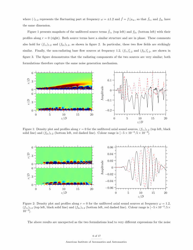
where (·)1.2 represents the fluctuating part at frequency ω = ±1.2 and f = f/ρ∞, so that f1z and f2z have

the same dimension.

Figure 1 presents snapshots of the unfiltered source terms f1z (top left) and f2z (bottom left) with their

profiles along r = 0 (right). Both source terms have a similar structure and are in phase. These comments

also hold for (f1z)1.2 and (f2z)1.2, as shown in figure 2. In particular, these two flow fields are strikingly

similar. Finally, the non-radiating base flow sources at frequency 1.2, (f1z)′1.2 and (f2z)

′1.2, are shown in

figure 3. The figure demonstrates that the radiating components of the two sources are very similar; both

formulations therefore capture the same noise generation mechanism.

0

3

6

r/D

0

3

6

r/D

0 5 10 15 20z/D

−0.2

−0.1

0

0.1

Amplitude

0 5 10 15 20z/D

Figure 1: Density plot and profiles along r = 0 for the unfiltered axial sound sources, (f1z)1.2 (top left, blacksolid line) and (f2z)1.2 (bottom left, red dashed line). Colour range is [−5× 10−3; 5× 10−3].

0

3

6

r/D

0

3

6

r/D

0 5 10 15 20z/D

−0.06

−0.04

−0.02

0

0.02

0.04

0.06

Amplitude

0 5 10 15 20z/D

Figure 2: Density plot and profiles along r = 0 for the unfiltered axial sound sources at frequency ω = 1.2,(f1z)1.2 (top left, black solid line) and (f2z)1.2 (bottom left, red dashed line). Colour range is [−5×10−3; 5×10−3].

The above results are unexpected as the two formulations lead to very different expressions for the noise

6 of 17


0

3

6

r/D

0

3

6

r/D

0 5 10 15 20z/D

−2

−1

0

1

2

Amplitude×

10−4

0 5 10 15 20z/D

Figure 3: Density plot and profiles along r = 0 for the filtered axial sound sources at frequency ω = 1.2,(f1z)

′1.2 (top left, black solid line) and (f2z)

′1.2 (bottom left, red dashed line). Colour range is [−5×10−5; 5×

10−5].

sources: as shown by equation (17), the density-based formulation involves only the axial velocity and the

axial velocity gradient (vz and ∂vz/∂z), while the enthalpy-based formulation involves the radial velocity,

the gradient of axial velocity in the radial direction, and the gradient of radial velocity in the axial direction

(vr, ∂vr/∂z and ∂vz/∂r).

C. Radial sound sources

Similarly, the radial source terms can be approximate by

f ′1r ≈∂

∂r(ρ vrvr)

′, f ′2r ≈ −(Ωvz)′ = −


∂z

)vz

]′. (18)

Since we know from8 that the dominant noise mechanism is related to velocity fluctuations rather than

density fluctuations, we will use the approximation ρ ≈ ρ∞ in the expression of f1z, i.e.

f ′1r/ρ∞ ≈∂

∂r(vrvr)

′, f ′2r ≈ −[(

∂vz∂r− ∂vr

∂z

)vz

]′. (19)

Finally, the filter can be applied frequency by frequency. The resulting source at frequency ω = 1.2 is given

by

(f1r)′1.2 ≈

∂

∂r(vrvr)

′1.2, (f2r)

′1.2 ≈


∂z

)vz

]′1.2

, (20)

where (·)1.2 represents the fluctuating part at frequency ω = ±1.2 and f = f/ρ∞, so that f1r and f2r have

the same dimension.

7 of 17


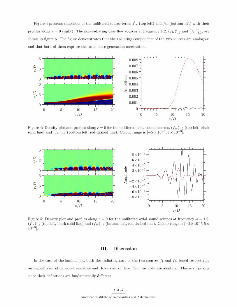
Figure 4 presents snapshots of the unfiltered source terms f1r (top left) and f2r (bottom left) with their

profiles along r = 0 (right). The non-radiating base flow sources at frequency 1.2, (f1r)′1.2 and (f2r)

′1.2, are

shown in figure 6. The figure demonstrates that the radiating components of the two sources are analogous

and that both of them capture the same noise generation mechanism.

0

3

6

r/D

0

3

6

r/D

0 5 10 15 20z/D

0

0.001

0.002

0.003

0.004

0.005

0.006

0.007

0.008

Amplitude

0 5 10 15 20z/D

Figure 4: Density plot and profiles along r = 0 for the unfiltered axial sound sources, (f1z)1.2 (top left, blacksolid line) and (f2z)1.2 (bottom left, red dashed line). Colour range is [−5× 10−3; 5× 10−3].

0

3

6

r/D

0

3

6

r/D

0 5 10 15 20z/D

−8×10−5

−6×10−5

−4×10−5

−2×10−5

0

2×10−5

4×10−5

6×10−5

8×10−5

Amplitude

0 5 10 15 20z/D

Figure 5: Density plot and profiles along r = 0 for the unfiltered axial sound sources at frequency ω = 1.2,(f1z)1.2 (top left, black solid line) and (f2z)1.2 (bottom left, red dashed line). Colour range is [−5×10−3; 5×10−3].

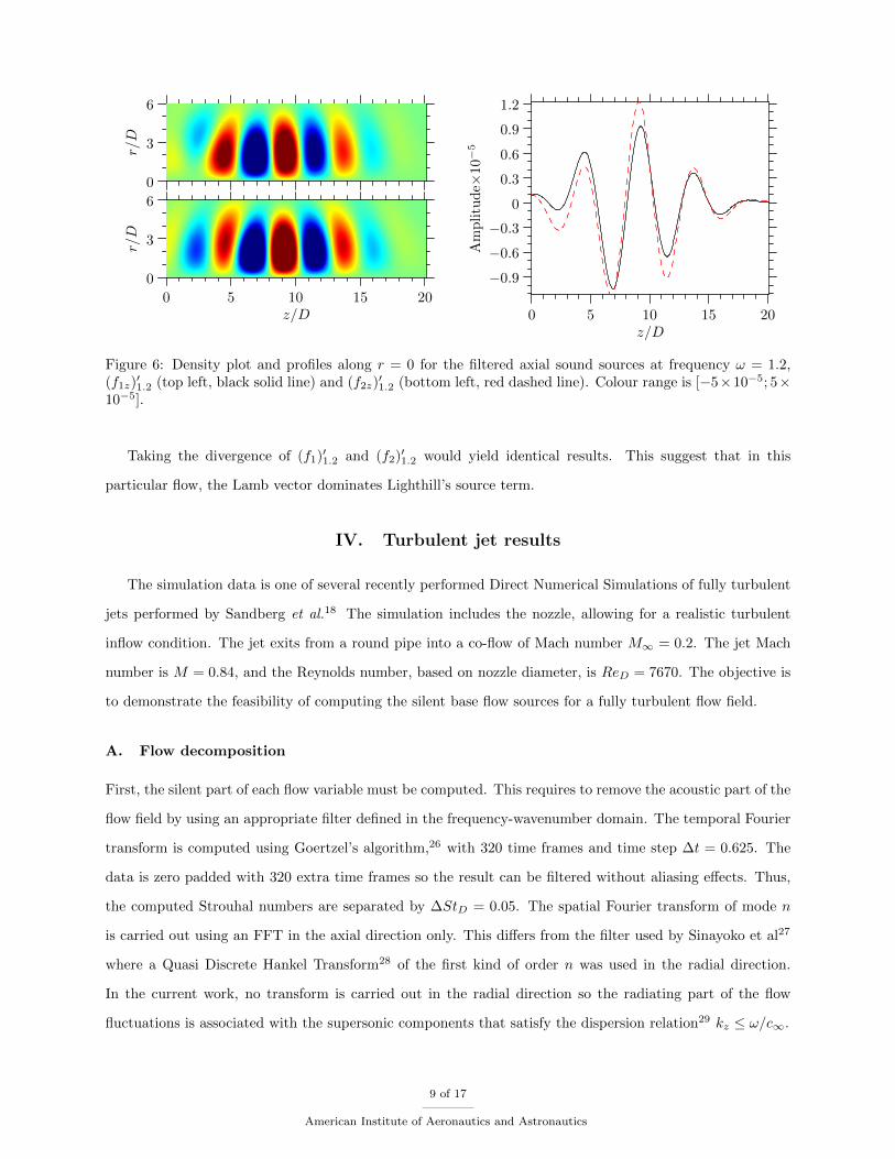
III. Discussion

In the case of the laminar jet, both the radiating part of the two sources f1 and f2, based respectively

on Lightill’s set of depedent variables and Howe’s set of dependent variable, are identical. This is surprising

since their definitions are fundamentally different.

8 of 17


0

3

6

r/D

0

3

6

r/D

0 5 10 15 20z/D

−0.9

−0.6

−0.3

0

0.3

0.6

0.9

1.2

Amplitude×

10−5

0 5 10 15 20z/D

Figure 6: Density plot and profiles along r = 0 for the filtered axial sound sources at frequency ω = 1.2,(f1z)

′1.2 (top left, black solid line) and (f2z)

′1.2 (bottom left, red dashed line). Colour range is [−5×10−5; 5×

10−5].

Taking the divergence of (f1)′1.2 and (f2)′1.2 would yield identical results. This suggest that in this

particular flow, the Lamb vector dominates Lighthill’s source term.

IV. Turbulent jet results

The simulation data is one of several recently performed Direct Numerical Simulations of fully turbulent

jets performed by Sandberg et al.18 The simulation includes the nozzle, allowing for a realistic turbulent

inflow condition. The jet exits from a round pipe into a co-flow of Mach number M∞ = 0.2. The jet Mach

number is M = 0.84, and the Reynolds number, based on nozzle diameter, is ReD = 7670. The objective is

to demonstrate the feasibility of computing the silent base flow sources for a fully turbulent flow field.

A. Flow decomposition

First, the silent part of each flow variable must be computed. This requires to remove the acoustic part of the

flow field by using an appropriate filter defined in the frequency-wavenumber domain. The temporal Fourier

transform is computed using Goertzel’s algorithm,26 with 320 time frames and time step ∆t = 0.625. The

data is zero padded with 320 extra time frames so the result can be filtered without aliasing effects. Thus,

the computed Strouhal numbers are separated by ∆StD = 0.05. The spatial Fourier transform of mode n

is carried out using an FFT in the axial direction only. This differs from the filter used by Sinayoko et al27

where a Quasi Discrete Hankel Transform28 of the first kind of order n was used in the radial direction.

In the current work, no transform is carried out in the radial direction so the radiating part of the flow

fluctuations is associated with the supersonic components that satisfy the dispersion relation29 kz ≤ ω/c∞.

9 of 17


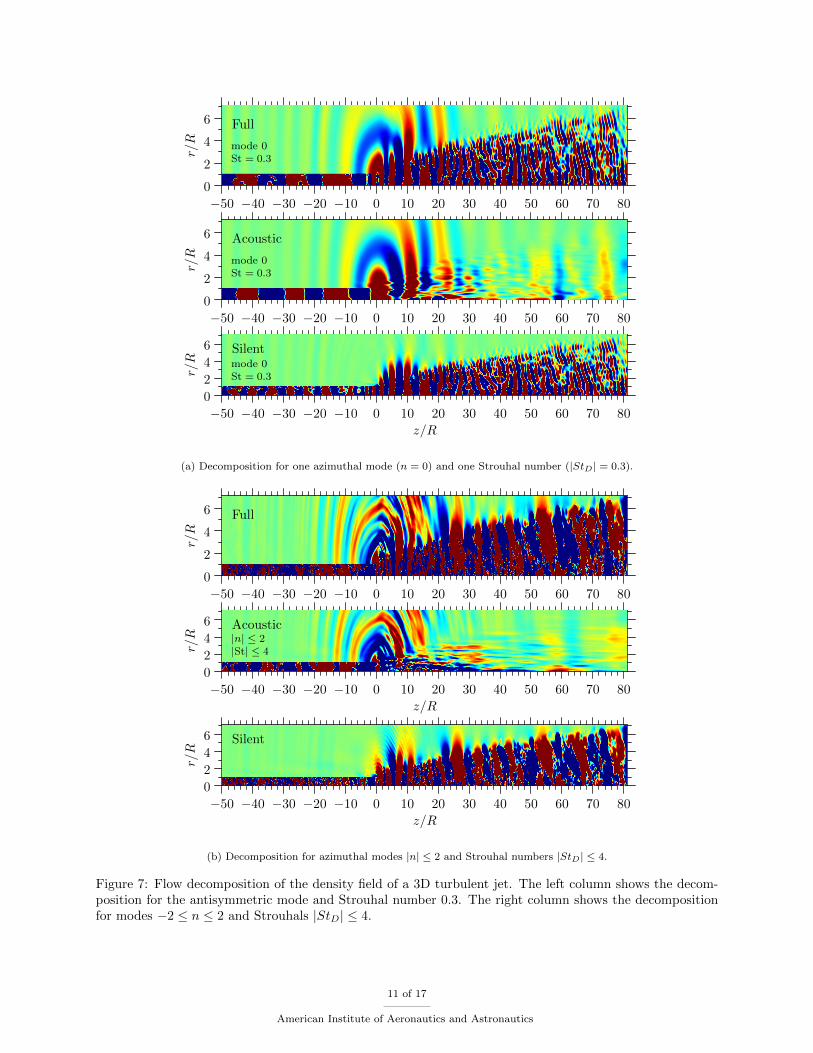
Figure 7 gives an overview of the flow decomposition. The 3D jet can be expressed as a series of

azimuthal modes. For each azimuthal mode, the flow field is essentially 2D so that the techniques developed

by Sinayoko et al8 can be applied. Thus, figure 7(a) shows how the acoustic part can be computed for

a particular azimuthal mode and Strouhal number. We similarly compute the acoustic part for Strouhal

numbers |St| ≤ 4 (with ∆St = 0.05) and azimuthal modes |n| ≤ 2 to obtain a good approximation of the

total acoustic part of the density field. As illustrated in figure 7(b) we can thereby obtain the non-radiating

density field ρ. We repeat the same process to get vr and vz.

B. Axial silent base flow source validation

The axial silent base flow source is approximated as (f1zz)′ = ∂z(ρvz vz)

′. It is computed for the axisymmetric

mode and Strouhal St = 0.3 in figure 8(a). The linearised Euler equations are then used to propagate the

sound source and the sound pressure level is compared with the exact result measured from the direct

numerical simulation. A comparison of the sound pressure level directivity is shown in figure 7(b).

The two results are in excellent agreement for angles θ ≤ 30. This is the region where wavepackets are

thought to be the dominant noise generation mechanism. For higher angles, the agreement is poor. The

reason is likley to be that only the zz-part of the axial sound sources has been used. The rr-part of the

radial source term is thought to be responsible for noise radiation towards higher angles.

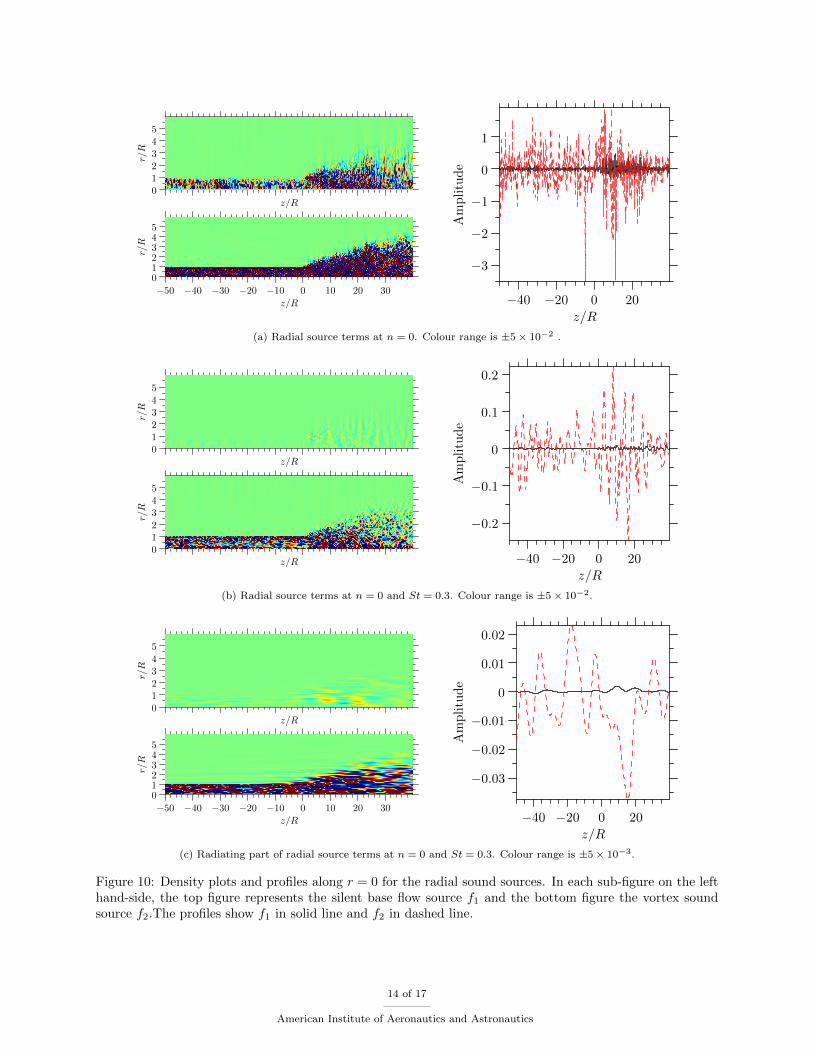
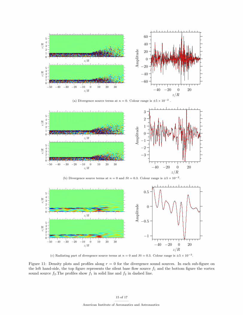
C. Sound sources comparison

We compute the sound source f2 in a similar way and compare it to f1. We compare the axial sources

f1z and f2z, the radial sources f1r and f2r, and their divergence ∇f1 and ∇f2, in figures 9,10 and 11. In

each figure, three successive subfigures present: (a) the unfiltered sources; (b) their component at Strouhal

St = 0.3; (c) their radiating component at that same frequency. In each case, the left column shows f1 on

top and f2 at the bottom, with their respective profile in the right column.

From figure 9 it is clear that the axial sources f1z and f2z are very different: source f1z has a much larger

amplitude. An analogous result can be seen in the case of the radial source f1r and f2r, but in this case it

is f2r that has the largest amplitude. These results are different from the ones obtained for the laminar jet,

for which the sources were in agreement in both the axial and radial directions.

Figure 11 compares the divergence of f1 and f2. These are found to be in perfect agreement at Strouhal

St = 0.3. This result suggest that in this flow and at that frequency, the axisymmetric mode of Lighthill’s

source term is dominanted by the Lamb vector. In other words, the additional terms, which are given by

f1 − f2 = (∇v) · v +1

2∇(v2z + v2r), (21)

10 of 17


0

2

4

6

r/R

−50 −40 −30 −20 −10 0 10 20 30 40 50 60 70 80

Full

mode 0St = 0.3

0

2

4

6

r/R

−50 −40 −30 −20 −10 0 10 20 30 40 50 60 70 80

Acoustic

mode 0St = 0.3

0

2

4

6

r/R

−50 −40 −30 −20 −10 0 10 20 30 40 50 60 70 80

z/R

Silentmode 0St = 0.3

(a) Decomposition for one azimuthal mode (n = 0) and one Strouhal number (|StD| = 0.3).

0

2

4

6

r/R

−50 −40 −30 −20 −10 0 10 20 30 40 50 60 70 80

Full

0

2

4

6

r/R

−50 −40 −30 −20 −10 0 10 20 30 40 50 60 70 80

z/R

Acoustic|n| ≤ 2|St| ≤ 4

0

2

4

6

r/R

−50 −40 −30 −20 −10 0 10 20 30 40 50 60 70 80

z/R

Silent

(b) Decomposition for azimuthal modes |n| ≤ 2 and Strouhal numbers |StD| ≤ 4.

Figure 7: Flow decomposition of the density field of a 3D turbulent jet. The left column shows the decom-position for the antisymmetric mode and Strouhal number 0.3. The right column shows the decompositionfor modes −2 ≤ n ≤ 2 and Strouhals |StD| ≤ 4.

11 of 17


0

1

r/R

−50 −40 −30 −20 −10 0 10 20 30

z/R

(a) Axial silent base flow source (f1zz)′ = ∂z(ρvz vz)′St=0.3

15

30

45

6075

0 (deg)

90

-3-63-123

Density, dB

(b) Sound pressure level at R = 60D:DNS (circles); LEE (solid)

Figure 8: Silent base flow source computation and validation for mode n = 0 and Strouhal StD = 0.3.

play a minor role in the noise generation process.

Conclusions

We have defined a new version of the silent base flow analogy based on Doak’s argument11 that total

enthalpy is the main acoustic variable. We have compared the resulting sound source, the radiating part of

the Lamb vector, to the one defined from the non-radiating base flow formulation of Lighthill’s analogy.8

The conclusion is that both definitions identify the same noise mechanism, despite having fundamentally

different expressions. In particular, the divergence of the two source terms have been found to be identical

for both the laminar jet and the fully turbulent jet.

However, in the case of the turbulent jet, the the mechanism by which each source operates on the

momentum equation appears different: the Lamb vector is found to excite primarily the radial momentum

equation, whereas Lighthill’s source excites primarily the axial direction.

Acknowledgements

The authors wish to acknowledge the contribution of Andre Cavalieri for stimulating discussions on the

interpretion of the computed noise sources during his stay as a David Crighton Fellow at the University of

Cambridge.

References

1Lighthill, M. J., “On sound generated aerodynamically. I. General theory,” Proceedings of the Royal Society of London,

Vol. 211, No. 1107, 1952, pp. 564–587.

2Lilley, G. M., “The generation and radiation of supersonic jet noise. Vol. IV - theory of turbulence generated jet noise,

noise radiation from upstream sources, and combustion noise. Part II: Generation of sound in a mixing region,” US Air Force

12 of 17


012345

r/R

z/R

012345

r/R

−50 −40 −30 −20 −10 0 10 20 30

z/R

−1

0

1

2

Amplitude

−40 −20 0 20

z/R

(a) Axial source terms at n = 0. Colour range is ±5× 10−2 .

012345

r/R

z/R

012345

r/R

−50 −40 −30 −20 −10 0 10 20 30

z/R

0

0.1

Amplitude

−40 −20 0 20

z/R

(b) Axial source terms at n = 0 and St = 0.3. Colour range is ±5× 10−2.

012345

r/R

z/R

012345

r/R

−50 −40 −30 −20 −10 0 10 20 30

z/R

−0.02

−0.01

0

0.01

0.02

Amplitude

−40 −20 0 20

z/R

(c) Radiating part of axial source terms at n = 0 and St = 0.3. Colour range is ±5× 10−3.

Figure 9: Density plots and profiles along r = 0 for the axial sound sources. In each sub-figure on the lefthand-side, the top figure represents the silent base flow source f1 and the bottom figure the vortex soundsource f2. The profiles show f1 in solid line and f2 in dashed line.

13 of 17


012345

r/R

z/R

012345

r/R

−50 −40 −30 −20 −10 0 10 20 30

z/R

−3

−2

−1

0

1

Amplitude

−40 −20 0 20

z/R

(a) Radial source terms at n = 0. Colour range is ±5× 10−2 .

012345

r/R

z/R

012345

r/R

z/R

−0.2

−0.1

0

0.1

0.2

Amplitude

−40 −20 0 20

z/R

(b) Radial source terms at n = 0 and St = 0.3. Colour range is ±5× 10−2.

012345

r/R

z/R

012345

r/R

−50 −40 −30 −20 −10 0 10 20 30

z/R

−0.03

−0.02

−0.01

0

0.01

0.02

Amplitude

−40 −20 0 20

z/R

(c) Radiating part of radial source terms at n = 0 and St = 0.3. Colour range is ±5× 10−3.

Figure 10: Density plots and profiles along r = 0 for the radial sound sources. In each sub-figure on the lefthand-side, the top figure represents the silent base flow source f1 and the bottom figure the vortex soundsource f2.The profiles show f1 in solid line and f2 in dashed line.

14 of 17


012345

r/R

z/R

012345

r/R

−50 −40 −30 −20 −10 0 10 20 30

z/R

−60

−40

−20

0

20

40

60

Amplitude

−40 −20 0 20

z/R

(a) Divergence source terms at n = 0. Colour range is ±5× 10−2 .

012345

r/R

z/R

012345

r/R

−50 −40 −30 −20 −10 0 10 20 30

z/R

−3

−2

−1

0

1

2

3

Amplitude

−40 −20 0 20

z/R

(b) Divergence source terms at n = 0 and St = 0.3. Colour range is ±5× 10−2.

012345

r/R

z/R

012345

r/R

−50 −40 −30 −20 −10 0 10 20 30

z/R

−1

−0.5

0

0.5

Amplitude

−40 −20 0 20

z/R

(c) Radiating part of divergence source terms at n = 0 and St = 0.3. Colour range is ±5× 10−3.

Figure 11: Density plots and profiles along r = 0 for the divergence sound sources. In each sub-figure onthe left hand-side, the top figure represents the silent base flow source f1 and the bottom figure the vortexsound source f2.The profiles show f1 in solid line and f2 in dashed line.

15 of 17


Aero Propulsion Lab., AFAPL-TR-72-53, July, 1972.

3Howe, M. S., “Contributions to the theory of aerodynamic sound, with application to excess jet noise and the theory of

the flute,” Journal of Fluid Mechanics, Vol. 71, 1975, pp. 625 – 73.

4Bogey, C., Bailly, C., and Juve, D., “Computation of flow noise using source terms in linearized Euler’s equations,” AIAA

Journal , Vol. 40, No. 2, 2002, pp. 235–243.

5Goldstein, M. E., “A generalized acoustic analogy,” Journal of Fluid Mechanics, Vol. 488, 2003, pp. 315–333.

6Goldstein, M. E., “On identifying the true sources of aerodynamic sound,” Journal of Fluid Mechanics, Vol. 526, 2005,

pp. 337–347.

7Sinayoko, S., Agarwal, A., and Hu, Z., “Flow decomposition and aerodynamic noise generation,” Journal of Fluid

Mechanics, Vol. 668, 2011, pp. 335–350.

8Sinayoko, S. and Agarwal, A., “On computing the physical sources of sound in a laminar jet,” .

9Suponitsky, V., Sandham, N. D., and Morfey, C. L., “Linear and nonlinear mechanisms of sound radiation by instability

waves in subsonic jets,” Journal of Fluid Mechanics, Vol. 658, June 2010, pp. 509–538.

10Powell, A., “Theory of vortex sound,” The journal of the acoustical society of America, Vol. 36, 1964, pp. 177.

11Doak, P., “Fluctuating Total Enthalpy as the Basic Generalized Acoustic Field,” Theoretical and Computational Fluid

Dynamics, Vol. 10, No. 1-4, Jan. 1998, pp. 115–133.

12Ffowcs Williams, J. E. and Hawkings, D. L., “Sound generation by turbulence and surfaces in arbitrary motion,” Philo-

sophical Transactions for the Royal Society of London. Series A, Mathematical and Physical Sciences, Vol. 264, No. 1151,

1969, pp. 321–342.

13Morfey, C. L. and Wright, M. C. M., “Extensions of Lighthill’s acoustic analogy with application to computational

aeroacoustics,” Proceedings of the Royal Society of London, Series A (Mathematical, Physical and Engineering Sciences),

Vol. 463, No. 2085, 2007, pp. 2101–2127.

14Spalart, P. R. and Shur, M. L., “Variants of the Ffowcs Williams Hawkings equation and their coupling with simulations

of hot jets,” Vol. 8, No. 5, 2009, pp. 477–492.

15Howe, M. S., “Contributions to the theory of aerodynamic sound, with application to excess jet noise and the theory of

the flute,” Journal of Fluid Mechanics, Vol. 71, No. 04, March 2006, pp. 625.

16Ewert, R. and Schroder, W., “Acoustic perturbation equations based on flow decomposition via source filtering,” Journal

of Computational Physics, Vol. 188, No. 2, 2003, pp. 365–398.

17Suponitsky, V., Sandham, N. D., and Morfey, C. L., “Linear and nonlinear mechanisms of sound radiation by instability

waves in subsonic jets,” Journal of Fluid Mechanics, Vol. 658, 2010, pp. 509–538.

18Sandberg, R., Sandham, N. D., and Suponitsky, V., “DNS of a fully turbulent jet flows in flight conditions including a

canonical nozzle,” AIAA paper , 2011.

19Margnat, F., Fortune, V., Jordan, P., and Gervais, Y., “Decomposition of the Lighthill source term and analysis of

acoustic radiation from mixing layers.” The Journal of the Acoustical Society of America, Vol. 123, No. 5, 2008.

20Howe, M. S., Theory of vortex sound , Cambridge Univ Pr, 2003.

21Crighton, D. G., “Basic principles of aerodynamic noise generation,” Progress in Aerospace Sciences, Vol. 16, 1975,

pp. 31–96.

22Bogey, C., Bailly, C., and Juve, D., “Noise investigation of a high subsonic, moderate Reynolds number jet using a

compressible large eddy simulation,” Theoretical and Computational Fluid Dynamics, Vol. 16, No. 4, 2003, pp. 273–297.

23Tam, C. K. W., “Supersonic jet noise,” Annual Review of Fluid Mechanics, Vol. 27, 1995, pp. 17–43.

16 of 17


24Stromberg, J. L., McLaughlin, D. K., and Troutt, T. R., “Flow field and acoustic properties of a Mach number 0.9 jet at

a low Reynolds number,” Journal of Sound and Vibration, Vol. 72, No. 2, 1980, pp. 159–176.

25Suponitsky, V. and Sandham, N. D., “Nonlinear mechanisms of sound radiation in a subsonic flow,” AIAA paper 2009-

3317 , 2009.

26Goertzel, G., “An algorithm for the evaluation of finite trigonometric series,” The American Mathematical Monthly,

Vol. 65, No. 1, 1958, pp. 34–35.

27Sinayoko, S., Agarwal, A., and Sandberg, R., “Physical sources of sound in laminar and turbulent jets,” AIAA paper

2011-2916 , 2011.

28Guizar-Sicairos, M. and Gutierrez-Vega, J. C., “Computation of quasi-discrete Hankel transforms of integer order for

propagating optical wave fields,” Journal of the Optical Society of America A, Vol. 21, No. 1, 2004, pp. 53–58.

29Freund, J. B., “Noise sources in a low-Reynolds-number turbulent jet at Mach 0.9,” Journal of Fluid Mechanics, Vol. 438,

2001, pp. 277–305.

17 of 17


a comparison of the silent base ow and vortex sound

Documents