a comparison of two methods for measuring land … comparison of two methods for measuring land use...

A Comparison of Two Methods for Measuring Land Use in Public Health Research:

Systematic Social Observation vs. GIS-Based Coded Aerial Photography

Katherine E. King

Population Studies Center Research Report 12-772

September 2012

Katherine E. King is an ORISE Postdoctoral Researcher, Environmental Protection Agency, National Health and Environmental Effects Research Laboratory, and Visiting Assistant Professor, Department of Sociology, Duke University This research was supported in part by the Michigan Center for Integrative Approaches to Health Disparities (P60MD002249) funded by the National Center on Minority Health and Health Disparities and by a postdoctoral fellowship from the Center for the Study of Aging and Human Development at Duke University Medical Center funded by the National Institute on Aging (2T32 AG000029-35). The author gratefully acknowledges use of the services and facilities of the Population Studies Center at the University of Michigan, funded by NICHD Center Grant R24 HD041028. The author wishes to thank Philippa Clarke, Jeffrey Morenoff, Jim House, Jennifer Ailshire, and Robert Melendez for their comments.

Two Methods for Measuring Land Use in Public Health Research 2

ABSTRACT Public health researchers have identified numerous health implications associated with land use. However, it is unclear which of multiple methods of data collection most accurately capture land use, and “gold standard” methods vary by discipline. In this paper, five desirable features of ecological data sources are presented and discussed (cost, coverage, availability, construct validity, and accuracy). Potential accuracy issues are discussed by using Kappa statistics to evaluate the level of agreement between datasets collected by two methods (systematic social observation (SSO) by trained raters and publically available data from aerial photography coded using administrative records) from the same blocks in Chicago. Findings show that significant kappa statistics range from .19 to .60, indicating varying levels of inter-source agreement. Most land uses are more likely to be reported by researcher-designed direct observation than in the publicly available data derived from aerial photography. However, when cost, coverage, and availability outweigh a marginal improvement in accuracy and flexibility in land use categorization, coded aerial photography data may be a useful data source for health researchers. Greater interdisciplinary and inter-organization collaboration in the production of ecological data is recommended to improve cost, coverage, availability, and accuracy, with implications for construct validity. Abbreviations CMAP Chicago Metropolitan Authority for Planning CCAHS Chicago Community Adult Health Study SSO Systematic social observation GIS Geographic information systems


INTRODUCTION

The residential physical and built environment is considered an important domain of

health risk factors and opportunities. Ample literature in public health and sociology

demonstrates “neighborhood effects,” associations of neighborhood features such as

socioeconomic disadvantage, affluence, and race/ethnic composition on health. Recent research

emphasizes moving beyond correlations between neighborhood socioeconomic resources and

health to relate specific features of the environment to precise outcomes through well-defined

socio-biological processes.

Most importantly, health researchers, community sociologists, landscape ecologists, and

urban planners have focused considerable attention on how features of “walkability” (defined

various ways) influence physical activity. In particular, land use – the allocation of land to

different uses such as residential, commercial, industrial, open space, etc., and the mix and

density of these uses – is hypothesized to affect health through a number of mechanisms. By

shaping how people and goods move through an area, land use mix and intensity are said to

structure physical activity (Saelens and Handy 2008), access to health opportunities (Smiley et al.

2010), community social relations (Talen 1999), and exposure to crime (Hipp 2007) and

pollution (Frank and Engelke 2005). These and other sociobehavioral community characteristics

communities in turn influence land use change in a reciprocal process. Initial evidence for

associations between land use and health has largely been based on proxy variables (e.g.,

population density, commute time, or the occupational mix of persons employed in the area.)

Current work defining walkable urban form often includes three measures: residential density,

street connectivity, and an entropy measure of land use mix based on five categories (residential,

commercial, institutional, recreational, and other) (Frank et al. 2006).

Difficulty with ecological data collection has been a major focus of recent

interdisciplinary attention, but no consensus has been reached. Broadly speaking, planning

research often uses administrative records or remote sensing. Health researchers often use self-

reports or community surveys, which cluster self-reports of respondents’ (or an ancillary

samples’) surroundings. Urban sociologists tend to prefer systematic social observation

performed by trained raters who “hit the pavement” to record detailed information about

neighborhoods of interest. Analysis of any of these data types typically involves use of a


geographic information system (GIS) software package for visual and quantification display of

information.

The present study assesses the level of agreement between two data sources which

measure land use using two different “gold standard” methods: (1) systematic social observation

(SSO) by a trained rater, and (2) GIS-based coded aerial photography data about whether each of

eight types of land uses was present on 1,662 blocks in both 2002 SSO data from the Chicago

Community Adult Health Survey (CCAHS) and aerial photography data coded by the Chicago

Metropolitan Authority for Planning (CMAP; (Chicago Metropolitan Agency for Planning

2006)).

More research is needed to evaluate the accuracy of various ecological measurement

systems such as systematic social observation (Brownson et al. 2009). “Head-to-head”

comparisons across methods may be especially valuable. Clarke and colleagues (Clarke et al.

2010) compared a Google Street View-based neighborhood audit with SSO, finding high rates of

observed agreement and Kappa values ranging from .31 for presence of institutional land to .71

for high-rise housing. Bader and colleagues (Bader et al. 2010) compared the level of agreement

of SSO measures of the presence of neighborhood businesses with commercial database business

listings. Kappa values for various business types ranged from .32 to .70. Most business types

were more likely to be reported by the SSO, but the use of either data source could be reasonable,

depending on the situation.

COMPARING DATA SOURCES

Little evidence is currently available to guide researchers in selecting among potential

data sources. Existing sources of land use data vary in terms of (1) cost, (2) coverage,

availability, (3) construct validity, and (4) accuracy. Little information is available about relative

costs of various data collection methods. Data sources vary considerably in terms of coverage

and aggregability. Observations collected as part of a survey are usually conducted only at

sampled locations within the study area, such as near respondents’ homes, but it is not known

how sampled locations may differ from other non-sampled locations within the study area. Nor

is it known how accurately characteristics are measured when aggregating from small areas to a

larger area (such as when blocks are aggregated to characterize the census tract level). Many

observational and administrative data sources specify a precise spatial scale, such as census tracts


or housing units, which confine analysis to administrative boundaries and complicate

investigation of spatial scale. Data collected by aerial photography or satellite imagery has a

potential advantage in terms of coverage if it is available and consistently measured for the entire

study site as a continuous surface rather than within particular geographic boundaries.

Availability of appropriate data is another issue. When the researcher seeks to

supplement an existing dataset, GIS-based and administrative measures are likely the only

measures of ecological characteristics available which include land use. Ideally, observation of

time-variant ecological measures occurs at the same time as or before collection of individual-

level data. Even when such administrative data exists, it may be difficult for the researcher to

obtain, and its temporal relationship to survey data is largely a function of administrative rather

than research concerns. By contrast, satellite imagery and aerial photography do not require

travel to the study site, which make them potentially appropriate when supplementing surveys

which cover large spaces, especially those which do not involve on-site interviews. Remote

methods are also unlikely to require institutional review board approval. Collecting

observational data offers a researcher control when access to other sources of data is uncertain.

Both secondary data sources and observational methods offer challenges in terms of

construct validity. Categorization of the built environment and land use should be based on

hypotheses about the effects of precise features of the environment. This is a challenge when

collection of data related to the built environment is time-intensive, given the rapid development

of social ecological theory during the last decade. Hence, categorizations used in various SSO’s

differ. Even when the choice of category codes is consistent, the physical reality of the built

environment may not be easy to classify. In some cases, the actual use of a property might not

match the exterior appearance (e.g. a law office in a converted church) or the ownership (e.g. an

industrial facility purchased by the adjacent university). In these cases, it may not be clear which

use suggests the appropriate coding for health purposes: the visual categorization which might

affect the stress levels of passers-by, the categorization which might affect employment levels,

etc.

Secondary sources may require considerable validation and probing because they were

not designed for health and social research. For instance, when social scientists conduct

household listings as a preliminary to survey sampling, they try to consider all the possible

places people might live, such as an apartment over a store. Land use data designed for


commercial or planning purposes, on the other hand, may not focus on capturing secondary

residential uses of commercial properties, even when changing the primary land use by re-zoning,

widening a road, or selling the property would change the secondary use. Likewise, “off the

books” uses of residential or other land for commercial purposes (Schaefer-McDaniel, Caughy,

O’Campo, & Gearey, 2010) which may be observed at the street level, might not appear in

records or be visible from the air. On the other hand, planners and developers might be

interested in more detailed categories of industrial properties than would social survey designers,

and that information might turn out to be useful to health researchers. Each group might learn

from the other.

More research is needed to evaluate the accuracy of various ecological measurement

systems such as systematic social observation (Brownson, Hoehner, Day, Forsyth, & Sallis,

2009). “Head-to-head” comparisons across methods may be especially valuable. Clarke and

colleagues (2010) compared a Google Street View based neighborhood audit with an SSO,

finding high rates of observed agreement and Kappa values ranging from .31 for presence of

institutional land to .71 for presence of high-rise housing. Bader and colleagues (2010)

compared the level of agreement between SSO measures of the presence of neighborhood

businesses and listings of businesses from commercial databases. Kappa values for different

business types ranged from .32 to .70. Most business types were more likely to be reported by

the SSO, but the use of either data source could be reasonable, depending on the situation.

METHODS

The goal of the paper is to evaluate the level of agreement between data collected by two

methods from the same blocks in Chicago, Illinois. One dataset comes from a systematic social

observation (SSO) by trained raters as a component of a large study of the social determinants of

health. The second is a publically downloadable dataset based on aerial photography and coded

using administrative records for use by local urban planners.

SSO Data

The SSO conducted for the CCAHS, which is a multistage area probability sample of

3,105 adults in the city of Chicago during 2001-2003. A trained observer rated each of the 1,662

blocks on which at least one sampled respondent lived, with two raters providing evidence of


agreement for a subset of blocks. The rater walked around a block twice, first observing the

(usually four) sides of the block, and then observing the adjacent areas facing the block. Block

ratings included assessments of the physical condition of the buildings, street, amenities, and

perceived physical and social conditions, as well as housing, commercial, and overall land use

typologies. The present study focuses on ratings of land use and housing types.

Aerial Photography Data

The 2001 Land-use Inventory (CMAP, 2006) was compiled by the Chicago Area

Authority for Planning. The data collection was designed to contribute to long-range population,

household, employment, land use, and transportation planning conducted by CMAP. CMAP

scanned and digitized aerial photographs and manually traced outlines of land uses in ArcGIS,

using supplemental GIS and address list data to verify land use and location of boundaries, with

extensive cross-checks reported in the data documentation. Discrepancies were further

investigated.

Creating Comparability between Datasets

To create comparable measures between the two sources, we created Census block-level

dichotomous measures of the presence of each type of land use which was found in both data

sources, including secondary land uses from CMAP. To maximize comparability, we recoded

the CMAP land uses to approximate the SSO land use categories (residential, commercial/

business/ professional, industrial/ warehouse/ manufacturing, parking lots, open space and vacant

space, institutional, recreational, and waterfront.) Because SSO raters consider adjacent block

faces when coding blocks, we considered land uses in the CMAP which fell within a 40 foot

buffer around the Census block boundaries as being present on that block.

Table 1 shows descriptions of land use categories. The SSO categorized dwellings into

nine categories: (1) high-rise public apartments, (2) high-rise private apartments, (3) low-rise

public apartments, (4) low-rise private apartments, (5) two-family houses/duplexes, (6) row

houses/townhouses, (7) housing above commercial properties, (8) houses converted to

apartments, and (9) single family homes. The CMAP reported only four: (1) single, duplex, and

townhouse units, (2) multi-family units, (3) farmhouses, and (4) trailer park/mobile home units,

with farmhouses not present in the sampled blocks and only one block containing mobile home


units. Two categories of residences were thus created based on comparison of SSO and CMAP

housing categories: single household/single entry homes, and multiple household/shared entry

homes.

As with comparison of any two datasets created by different organizations, there are

limitations in comparability. Rather than being a weakness of the present study, the difficulty in

comparison underscores the need for research on data collection. Although the CMAP reports a

limited set of secondary land uses, in practice the data do not include any location where housing

and other land uses are combined which corresponds to the SSO’s category of housing above

commercial property. This likely results from two factors. First, because the data are designed

for planning rather than social survey purposes, the project was likely less concerned with

secondary land uses. Second, the data result from aerial photography, which might fail to

capture side entrances, vertical stacking, and other features which might be visible from the

ground. Results from sensitivity analyses not shown support this categorization.

The commercial/business/professional category from the SSO is considered to be

analogous to the following CMAP categories present in the sampled blocks: (1) retail centers, (2)

office campuses/research parks, (3) single structure office buildings, (4) business parks, (5 and 6)

urban mix with or without dedicated parking, and (7) hotels/motels. The manufacturing/

industrial/ processing category in the SSO is compared to the manufacturing and processing,

warehousing/distribution center and wholesale, industrial park, and utilities and waste facilities

from the CMAP. The institutional category from the SSO was simulated by combining

medical/health care, educational, government/administrative, religious, and “other facilities”

from CMAP.

The SSO parking lot category does not have a direct counterpart in CMAP. Here we

assume that parking lots are present in areas categorized by CMAP as urban mix with dedicated

parking and combine this with independent parking lots to produce a measure indicating parking

presence. Because SSO raters stand at the block face to code parking lots, they may not note

presence of parking lots behind buildings. CMAP, by contrast, would not be expected to report

parking lots on block faces such as for apartment or office buildings, institutions, etc., not coded

as “urban mix”; these parking areas would be coded according to the purpose of the buildings

they belong to. Neither dataset would report on-street or vacant lot parking.


Characterization of vacant and open space provides additional challenges. The SSO’s

vacant and open space category does not specify whether construction is included. While

construction might be a frequent mode of land use change, and thus for discrepancies in land use

categorization across the short term, land under construction is not conceptually the same as

vacant land. We therefore omit the construction categories from the CMAP, and include only

the category “primarily recreational open space, golf courses, open space for conservation, linear

open space (i.e. bike paths), and other open space, as well as vacant space.”

We recreate the SSO recreational category using the CMAP’s categories including

cultural and entertainment facilities (cultural, public assembly, amusement, and recreational

facilities (including water-based facilities), as well as primarily recreational open space (which

overlaps with open space). Finally, the SSO waterfront category is compared to three CMAP

categories: rivers, streams, and canals; lakes, reservoirs, and lagoons; and the parts of Lake

Michigan which are intersected by other land uses (e.g. docks). Comparison can be complicated

because water, open space, and transportation land uses often co-occur. The SSO allows reports

of multiple uses; the rater may report water and open space if both are present, although no

category exists for transportation. By contrast, the CMAP reports only one category and may

select transportation or open space rather than water.

ANALYSES

We measure the degree of agreement between the two data sources and the extent to

which disagreement is related to sociodemographic characteristics of the neighborhood. The

degree of agreement between the two data sources on the presence of each land use type is

measured using kappa statistics, which report the inter-source reliability considering that some

agreement could be expected by chance. Specifically, the kappa statistic is the ratio of the

observed agreement to the expected agreement, based on the marginal frequencies in both data

sources. We use conventional benchmark categories for agreement (Landis and Koch 1977):

almost perfect (0.81-1.00), substantial (0.61-0.80), moderate (0.41-0.60), fair (0.21-0.40), and

slight (0.00-0.20).

Next, we consider whether disagreement between data sources might be higher when

land uses are less formal, such as informal commercial land uses in disadvantaged or Hispanic

neighborhoods (Venkatesh 2009). We expect the SSO would be more likely to report informal


land uses, because they would be visible at the street level but not in administrative records.

However, it might also be possible for administrative records to list a land use which did not

have external markings, resulting in a report in the CMAP but not in the SSO. Land use turnover

might also be higher in neighborhoods where residential stability is lower, making properties

difficult to code or resulting in category changes between the two data collection times. If

characteristics of neighborhoods are unrelated to disagreement between sources, researchers can

feel more confident in choosing either source.

To evaluate whether disagreement between the two sources is systematically related to

the sociodemographic characteristics of the neighborhood, we create a dichotomous indicator

variable for agreement for each block and fit logistic regression models which report the log-

odds of agreement about the presence of a particular land use on a block. We use four variables

in our analysis to describe tract-level socioeconomic composition, following Bader and

colleagues (Bader et al. 2010). The tract level data is preferred over block group data because of

a view that tracts are likely large enough that tracts may influence the presence of land uses

rather than land uses influencing nearby socioeconomic conditions. That is, a block group

containing a large factory might have low population density and socioeconomic status precisely

because of proximity to the factory, whereas this phenomenon should be somewhat smoothed out

at the tract level.

Neighborhood sociodemographic data come from Summary File 3 of the 2000 US

Census. The first scale is referred to as “neighborhood disadvantage” because it combines

measures of the proportion of households with incomes of less than $15,000 and incomes of at

least $50,000 (reverse coded), as well as rates of family poverty, public assistance,

unemployment, and vacant housing. The percentage non-Hispanic white and the

Hispanic/foreign born scale (which combines measures of the percentage of Hispanics and the

percentage foreign born) capture ethnic composition. The residential stability scale is composed

of the percent residing in their homes for five years or more and percent home ownership.

We also include a measure of distance in kilometers from Chicago’s central business

district (“The Loop” – specifically, the site where the Sears Tower was located) to the centroid of

the block polygon because certain land uses (e.g. shared-entry residential, commercial/ business/

professional) are more common closer to downtown, and this may influence the likelihood of

inter-source agreement. Failing to report a land use during coding (in either data source) when


that land use actually is present might also be more likely when more land uses are present

(Bader et al. 2010).

Finally, we include a variable indicating the time difference in months between the data

collections. About 10% of the systematic social observations occurred within 8 months of the

aerial photography, while about 90% occurred between 18 and 22 months later. Even on a two-

year time scale, we suspect that it will be relatively rare for land uses to completely change

categories, but available data do not allow us to quantify the impact of land use change on the

discrepancies. However, according to the CMAP, less than one percent of the sampled blocks

contained construction, and half of that construction was residential. Analyses of source

agreement exclude three blocks for which the SSO observation date was missing.

RESULTS

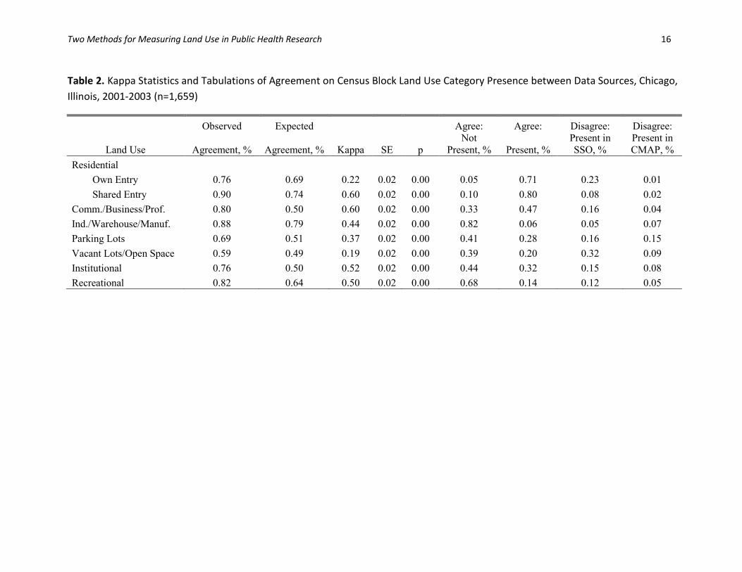
Table 2 reports the results of the correspondence analysis. The SSO and coded aerial

photography data display considerable agreement, which ranges from 90% (Κ=.60) for shared-

entry residential land use to 59% (Κ=.19) for vacant lots/open space o. Agreement about

industrial/ warehouse/ manufacturing land use (88%, Κ=.44) and shared entry housing (90%,

Κ=.60) was moderate. There was less agreement within the own-entry residential category (76%,

Κ=.22), although single-entry homes might be expected to be relatively simple to identify. This

is almost certainly due to disagreement about housing type category, particularly to the

ambiguity about houses converted to apartments. (There is disagreement about the presence of

any residential land for only 9 blocks, and agreement that there is no residence on one block.)

Institutional and recreational land uses 76% (Κ=.52) and 82% (Κ=.50) respectively) also show

moderate agreement. The level of agreement on the presence of parking lots (69%, Κ=.37) is

better than might be expected when considering that the CMAP data only reports certain

categories of parking lots (independent lots and lots associated with mixed urban commercial

use); we expect the SSO to report more parking lots associated with apartments, institutions,

offices, etc. All kappa values are significant, indicating more agreement than would be expected

by chance.

We then cross-tabulated reports of presence of each land use category by source. The last

four columns of Table 2 report the frequency of blocks on which 1) the land use is reported

present by both datasets, 2) the land use is not reported in either dataset, 3) only the SSO reports


the land use is present, and 4) only the CMAP reports the land use is present. Where

disagreement occurred, it was more commonly the case that only the SSO had reported the land

use rather than that only the CMAP had reported the land use. This is especially true for both

types of residential land uses and vacant lots/open space, although the datasets are about equally

likely to report industrial/warehouse/manufacturing and parking lot land uses, and water(front)

(which is present at low frequency).

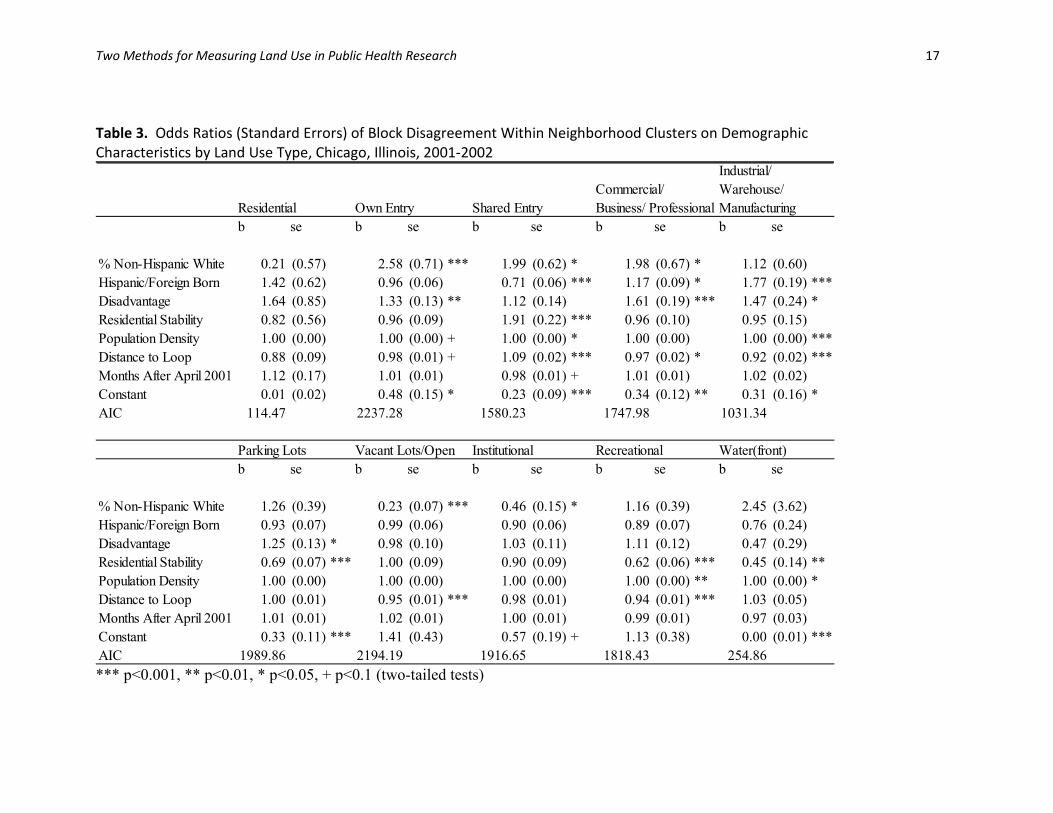
In Table 3, we report odds ratios estimated from the regression of block disagreement.

There were no clear and consistent patterns of association of sociodemographic variables with

coding disagreement. Only 25 of the 60 coefficients of sociospatial associations (with the 10

land uses) estimated were significant at P<0.05. There were no significant predictors of

disagreement on residential land use overall, but percent white predicted much more

disagreement on own entry and shared entry housing. Disadvantage predicted coding

discrepancies about own entry, while shared entry discrepancies were more common in

residentially stable areas and less common in Hispanic/foreign-born areas. Neighborhood-level

percent non-Hispanic white predicted less disagreement on institutional, commercial, and

vacant/open land uses, perhaps indicating more stable or larger institutions in white locales.

Also, Hispanic/foreign-born composition and disadvantage also predict disagreement on

commercial and industrial land uses, and disadvantage predicts less agreement on parking lots.

Residential stability predicts disagreement on shared entry housing, and predicts agreement on

parking lots, water(front) and recreational land use. Population density is associated with shared

entry, industrial, recreational, and water(front) land uses. Months elapsed between SSO and

CMAP data collections did not predict disagreement, a finding consistent with a limited role of

change over time as a source of disagreement. Distance from the downtown Loop area predicts

less disagreement on several land uses (shared entry housing, commercial, industrial,

vacant/open, and recreational), the same variables predicted by population density. The pseudo-

R2 values (ranging from .01 to .07) suggest that the socioeconomic characteristics, density, and

proximity of the neighborhood to the central business district predict very little of the

disagreement between sources.

As a follow-up to this analysis, visual comparison of sites where disagreement on

presence of water(front) occurred with a map of hydrological features around Chicago revealed

that all sites where intersource disagreements occurred were in fact in close proximity to water.


The SSO reports of water on 24 blocks where the CMAP did not report water were likely due to

the different data collection methods discussed above; it is unclear why the SSO did not report

waterfront on 5 blocks were adjacent to rivers.

DISCUSSION

We have demonstrated that when direct observational data is not available or does not

provide adequate coverage, publically available aerial photography-based data may be a good

option. For most land uses, there is a reasonably high agreement between the two sources, given

the difficulties involved in creating comparability. The SSO protocol resulted in reports of more

land uses than did the aerial photography method, and thus likely is more accurate. (An

assumption here is that false negatives are more common than false positives; that is, when

sources disagree, the land use probably is actually present.) Observed agreement was reasonable

for most land uses (>75%, except parking and open space), especially given that the categories

were not completely comparable across datasets. However, the Kappa coefficients were

considerably lower (.19-.60), which is expected when particular land uses are relatively rare.

The correspondence between the two datasets was also lower than in other comparability

research using the same Chicago SSO data (Clarke et al. 2010; Bader et al. 2010). However,

Bader and colleagues (Bader et al. 2010) examined only one type of land use (commercial

businesses), and had more information available to achieve comparability between data sources.

Geographic boundaries between parcels are much less clearly defined than administrative

boundaries between businesses. Clarke and colleagues’ (Bader et al. 2010) reports of

agreements on land use between the SSO data and observational coding by a trained rater using

Google Earth rely on the same categories, face rather than block level data, and the same

purposes in data collection.

Given the reasonable level of agreement between the two sources, decisions about what

kind of source to use will likely depend on other factors. Using existing administrative data is

inherently cheaper than collecting it. Validity of categories measured will depend on the

predictors and outcomes of interest, but lack of information about assumptions made in

categorization is a key challenge in comparing data sources. For this reason, we would urge the

use of more detailed descriptions of land use categories than are conventionally used, in order to

make coding more straightforward and also facilitate comparison of categories across studies.


In terms of coverage, remote sensing data is likely to excel: the SSO data is only

available for 1,662 of Chicago’s approximately 24,000 blocks, whereas CMAP data was

available for all of Chicago, as well as the surrounding counties. Data for outside city boundaries

is often needed when constructing contextual measures for locations near boundaries.

Our study contributes to research on ecological measurement. Analysis of the physical

environment in general, and land use in particular, is a rapidly emerging literature which holds

promise for health and urban planning policy. But in order to advance this research agenda, both

further research and additional insight is needed on data collection methodology.


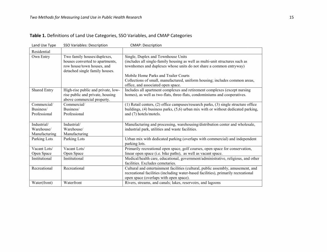
Table 1. Definitions of Land Use Categories, SSO Variables, and CMAP Categories

Land Use Type SSO Variables: Description CMAP: Description Residential

Own Entry Two family houses/duplexes, houses converted to apartments, row house/town houses, and detached single family houses.

Single, Duplex and Townhouse Units (includes all single-family housing as well as multi-unit structures such as townhomes and duplexes whose units do not share a common entryway) Mobile Home Parks and Trailer Courts Collections of small, manufactured, uniform housing; includes common areas, office, and associated open space.

Shared Entry High-rise public and private, low-rise public and private, housing above commercial property.

Includes all apartment complexes and retirement complexes (except nursing homes), as well as two-flats, three-flats, condominiums and cooperatives.

Commercial/ Business/ Professional

Commercial/ Business/ Professional

(1) Retail centers, (2) office campuses/research parks, (3) single structure office buildings, (4) business parks, (5,6) urban mix with or without dedicated parking, and (7) hotels/motels.

Industrial/ Warehouse/ Manufacturing


Manufacturing and processing, warehousing/distribution center and wholesale, industrial park, utilities and waste facilities.

Parking Lots Parking Lots Urban mix with dedicated parking (overlaps with commercial) and independent parking lots.

Vacant Lots/ Open Space

Vacant Lots/ Open Space

Primarily recreational open space, golf courses, open space for conservation, linear open space (i.e. bike paths), as well as vacant space.

Institutional Institutional Medical/health care, educational, government/administrative, religious, and other facilities. Excludes cemetaries.

Recreational Recreational Cultural and entertainment facilities (cultural, public assembly, amusement, and recreational facilities (including water-based facilities), primarily recreational open space (overlaps with open space).

Water(front) Waterfront Rivers, streams, and canals; lakes, reservoirs, and lagoons


Table 2. Kappa Statistics and Tabulations of Agreement on Census Block Land Use Category Presence between Data Sources, Chicago, Illinois, 2001-2003 (n=1,659)

Observed Expected Agree: Agree: Disagree: Disagree:

Land Use Agreement, % Agreement, % Kappa SE p Not

Present, % Present, % Present in SSO, %

Present in CMAP, %

Residential Own Entry 0.76 0.69 0.22 0.02 0.00 0.05 0.71 0.23 0.01 Shared Entry 0.90 0.74 0.60 0.02 0.00 0.10 0.80 0.08 0.02

Comm./Business/Prof. 0.80 0.50 0.60 0.02 0.00 0.33 0.47 0.16 0.04 Ind./Warehouse/Manuf. 0.88 0.79 0.44 0.02 0.00 0.82 0.06 0.05 0.07 Parking Lots 0.69 0.51 0.37 0.02 0.00 0.41 0.28 0.16 0.15 Vacant Lots/Open Space 0.59 0.49 0.19 0.02 0.00 0.39 0.20 0.32 0.09 Institutional 0.76 0.50 0.52 0.02 0.00 0.44 0.32 0.15 0.08 Recreational 0.82 0.64 0.50 0.02 0.00 0.68 0.14 0.12 0.05


Table 3. Odds Ratios (Standard Errors) of Block Disagreement Within Neighborhood Clusters on Demographic Characteristics by Land Use Type, Chicago, Illinois, 2001-2002

b se b se b se b se b se

% Non-Hispanic White 0.21 (0.57) 2.58 (0.71) *** 1.99 (0.62) * 1.98 (0.67) * 1.12 (0.60)Hispanic/Foreign Born 1.42 (0.62) 0.96 (0.06) 0.71 (0.06) *** 1.17 (0.09) * 1.77 (0.19) ***Disadvantage 1.64 (0.85) 1.33 (0.13) ** 1.12 (0.14) 1.61 (0.19) *** 1.47 (0.24) *Residential Stability 0.82 (0.56) 0.96 (0.09) 1.91 (0.22) *** 0.96 (0.10) 0.95 (0.15)Population Density 1.00 (0.00) 1.00 (0.00) + 1.00 (0.00) * 1.00 (0.00) 1.00 (0.00) ***Distance to Loop 0.88 (0.09) 0.98 (0.01) + 1.09 (0.02) *** 0.97 (0.02) * 0.92 (0.02) ***Months After April 2001 1.12 (0.17) 1.01 (0.01) 0.98 (0.01) + 1.01 (0.01) 1.02 (0.02)Constant 0.01 (0.02) 0.48 (0.15) * 0.23 (0.09) *** 0.34 (0.12) ** 0.31 (0.16) *AIC 114.47 2237.28 1580.23 1747.98 1031.34

b se b se b se b se b se

% Non-Hispanic White 1.26 (0.39) 0.23 (0.07) *** 0.46 (0.15) * 1.16 (0.39) 2.45 (3.62)Hispanic/Foreign Born 0.93 (0.07) 0.99 (0.06) 0.90 (0.06) 0.89 (0.07) 0.76 (0.24)Disadvantage 1.25 (0.13) * 0.98 (0.10) 1.03 (0.11) 1.11 (0.12) 0.47 (0.29)Residential Stability 0.69 (0.07) *** 1.00 (0.09) 0.90 (0.09) 0.62 (0.06) *** 0.45 (0.14) **Population Density 1.00 (0.00) 1.00 (0.00) 1.00 (0.00) 1.00 (0.00) ** 1.00 (0.00) *Distance to Loop 1.00 (0.01) 0.95 (0.01) *** 0.98 (0.01) 0.94 (0.01) *** 1.03 (0.05)Months After April 2001 1.01 (0.01) 1.02 (0.01) 1.00 (0.01) 0.99 (0.01) 0.97 (0.03)Constant 0.33 (0.11) *** 1.41 (0.43) 0.57 (0.19) + 1.13 (0.38) 0.00 (0.01) ***AIC 1989.86 2194.19 1916.65 1818.43 254.86

Residential Own Entry Shared EntryCommercial/ Business/ Professional


Water(front)RecreationalInstitutionalVacant Lots/Open Parking Lots

*** p<0.001, ** p<0.01, * p<0.05, + p<0.1 (two-tailed tests)


REFERENCES

Saelens BE, Handy SL. 2008. Built Environment Correlates of Walking: A Review. Medicine and Science in Sports and Exercise 40(7): S550-S566.

Smiley MJ, Diez Roux AV, Brines SJ, Brown DG, Evenson KR, Rodriguez DA. 2010. A Spatial Analysis of Health-Related Resources in Three Diverse Metropolitan Areas. Health & Place 16(5): 885-892.

Talen E. 1999. Sense of Community and Neighbourhood Form: An Assessment of the Social Doctrine of New Urbanism. Urban Studies 36(8): 1361-1379.

Hipp JR. 2007. Block, Tract, and Levels of Aggregation: Neighborhood Structure and Crime and Disorder as a Case in Point. American Sociological Review 72: 659-680.

Frank LD, Engelke P. 2005. Multiple Impacts of the Built Environment on Public Health: Walkable Places and the Exposure to Air Pollution. International Regional Science Review 28(2): 193-216.

Frank LD, Sallis JF, Conway TL, Chapman JE, Saelens BE, Bachman W. 2006. Many Pathways from Land Use to Health - Associations Between Neighborhood Walkability and Active Transportation, Body Mass Index, and Air Quality. Journal of the American Planning Association 72(1): 75-87.

Chicago Metropolitan Agency for Planning. 2006. Data Bulletin: 2001 Land-use Inventory for Northeastern Illinois. Available: http://www.cmap.illinois.gov/LandUseInventory2005.aspx?ekmensel=c580fa7b_8_16_15051_4 [accessed April 2010.

Brownson RC, Hoehner C, Day K, Forsyth A, Sallis JF. 2009. Measuring the Built Environment for Physical Activity: State of the Science. American Journal of Preventive Medicine 36(4S): S99-S123.

Clarke P, Ailshire J, Melendez R, Bader M. 2010. Using Google Earth to Conduct a Neighborhood Audit: Reliability of a Virtual Audit Instrument. Health & Place 16(6): 1224-1229.

Bader MDM, Ailshire JA, Morenoff JD, House JS. 2010. Measurement of the Local Food Environment: A Comparison of Existing Data Sources. American Journal of Epidemiology 171(5): 609-617.

Landis JR, Koch GG. 1977. The Measurement of Observer Agreement for Categorical Data. Biometrics 33(1): 159-174.

Venkatesh S. 2009. Off the Books: The Underground Economy of the Urban Poor: Harvard University Press.

a comparison of two methods for measuring land … comparison of two methods for measuring land use...

Documents