a complete guide to linux process scheduling · a complete guide to linux process scheduling nikita...
TRANSCRIPT

A complete guide to Linux
process scheduling
Nikita Ishkov
University of Tampere
School of Information Sciences
Computer Science
M.Sc. Thesis
Supervisor: Martti Juhola
February 2015
University of Tampere
School of Information Sciences
Computer Science
Nikita Ishkov
M.Sc. Thesis, 59 pages
February 2015
The subject of this thesis is process scheduling in wide purpose operating systems. For many years
kernel hackers all over the world tried to accomplish the seemingly infeasible task of achieving
good interaction on desktop systems and low latencies on heavily loaded server machines. Some
progress has been made in this area since the rise of free software, but, in opinion of many, it is still
far from perfect. Lots of beginner operating system enthusiasts find the existing solutions too
complex to understand and, in light of almost complete lack of documentation along with common
hostility of active kernel developers towards rookies, impossible to get hands on.
Anyone who has the courage to wade into the dragon infested layer that is the scheduler, should be
aware of the ideas behind current implementations before making any contributions. That is what
this thesis is about – showing how things work under the hood and how they developed to be like
this. Every decision behind each concept in a kernel of an OS has its history and meaning. Here I
will guide you through process scheduling mechanisms in currently stable Linux kernel as an object
lesson on the matter.
The work starts with an overview of the essentials of process abstraction in Linux, and continues
with detailed code-level description of scheduling techniques involved in past and present kernels.
Key words and terms: operating systems, Linux, process scheduler, CFS, BFS.
Table of contents
1. Introduction .......................................................................................................... 1
2. Basics ...................................................................................................................... 2
2.1 PROCESS .................................................................................................................................................. 2
2.2 SLUB ALLOCATOR ..................................................................................................................................... 6
2.3 LINKED LIST ............................................................................................................................................... 8
2.4 NOTES ON C ............................................................................................................................................ 11
3. Scheduling ........................................................................................................... 15
3.1 STRUCTURE ............................................................................................................................................ 16
3.2 INVOKING THE SCHEDULER ....................................................................................................................... 30
3.3 LINUX SCHEDULERS, A SHORT HISTORY LESSON ........................................................................................ 32
3.4 CFS ........................................................................................................................................................ 41
3.5 REAL-TIME SCHEDULER ............................................................................................................................ 48
3.6 BFS ........................................................................................................................................................ 51
4. Conclusion ........................................................................................................... 58
References .................................................................................................................. 59
1
1. Introduction
This thesis contains an extensive guide on how kernels of open source operating systems handle
process scheduling. As an example, latest stable version of Linux kernel (at the time of writing
3.17.2) is used. All references to the source code are used with respect to the version mentioned
above.
The code is mainly presented in C programming language, partly with GCC extensions. At some
points machine dependent assembly is used. Thus, a reader is expected to be familiar with basic
structure of operating systems’ design and principles along with impeccabile knowledge of
programming techniques.
This work can be considered as a further research of my Bachelor’s thesis, where I shed light on
how a process abstraction is presented in modern operating systems, process management and the
essentials of process scheduling in Linux kernel.
2
2. Basics
This chapter will go through the essential concepts of process representation in Linux kernel: what
is a process inside the system, how the system stores and manipulates processes, and how to
manage lists in Linux. In Section 2.2, we will discuss efficiency of kernel’s memory handling for
spawning and destroying processes. At the end of the chapter, some points on the C programming
language will be clarified.
2.1 Process
A process is a running program, which consists of an executable object code, usually read from
some hard media and loaded into memory. From the kernel’s point of view, however, there is much
more to the picture. An OS stores and manages additional information about any currently running
program: address space, memory mappings, open files for read/write operations, state of the
process, threads and more.
In Linux, an abstraction of process is, however, incomplete without discussing threads, sometimes
called light-weight processes. By definition, a thread is an execution context, or flow of execution, in
a process; thus, every process consists of at least one thread. A process, containing several
execution threads is said to be a multi-threaded process. Having more than one thread in a process
enables concurrent programming and, on multi-processor systems, true parallelism [1].
Each thread has its own id (thread id or TID), program counter, process stack and a set of registers.
What makes threads especially useful is that they share an address space between each other,
avoiding any kind of IPC (Inter Process Communication) channel (pipes, sockets, etc.) to
communicate. Execution flows can share information by using, say, global variables or data
structures, declared in the same .text segment. As threads are in the same address space, a thread
context switch is inexpensive and fast. Also creation and destruction is quick. Unlike fork(), no
new copy of the parent process is made. In fact, creation of a thread uses the same system call as
fork() does, only with different flags:
clone(CLONE_VM | CLONE_FS | CLONE_FILES | CLONE_SIGHAND, 0);
The code above does basically the same as a normal process creation would do, with the exception
that the address space (VM), file system information (FS), open files (FILES) and signal handlers
along with blocked signals (SIGHAND) will be shared.
3
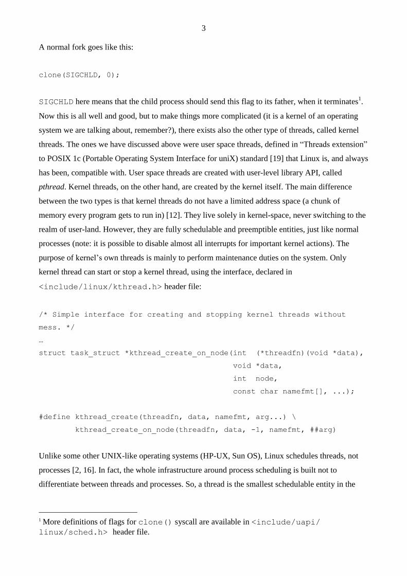
A normal fork goes like this:
clone(SIGCHLD, 0);
SIGCHLD here means that the child process should send this flag to its father, when it terminates1.
Now this is all well and good, but to make things more complicated (it is a kernel of an operating
system we are talking about, remember?), there exists also the other type of threads, called kernel
threads. The ones we have discussed above were user space threads, defined in “Threads extension”
to POSIX 1c (Portable Operating System Interface for uniX) standard [19] that Linux is, and always
has been, compatible with. User space threads are created with user-level library API, called
pthread. Kernel threads, on the other hand, are created by the kernel itself. The main difference
between the two types is that kernel threads do not have a limited address space (a chunk of
memory every program gets to run in) [12]. They live solely in kernel-space, never switching to the
realm of user-land. However, they are fully schedulable and preemptible entities, just like normal
processes (note: it is possible to disable almost all interrupts for important kernel actions). The
purpose of kernel’s own threads is mainly to perform maintenance duties on the system. Only
kernel thread can start or stop a kernel thread, using the interface, declared in
<include/linux/kthread.h> header file:
/* Simple interface for creating and stopping kernel threads without
mess. */
…
struct task_struct *kthread_create_on_node(int (*threadfn)(void *data),
void *data,
int node,
const char namefmt[], ...);
#define kthread_create(threadfn, data, namefmt, arg...) \
kthread_create_on_node(threadfn, data, -1, namefmt, ##arg)
Unlike some other UNIX-like operating systems (HP-UX, Sun OS), Linux schedules threads, not
processes [2, 16]. In fact, the whole infrastructure around process scheduling is built not to
differentiate between threads and processes. So, a thread is the smallest schedulable entity in the
1 More definitions of flags for clone() syscall are available in <include/uapi/
linux/sched.h> header file.
4
kernel [6]. Linux hackers use the word task as a synonym for process or thread, and so will we. The
kernel stores tasks in process descriptors (task_struct).
Process descriptor
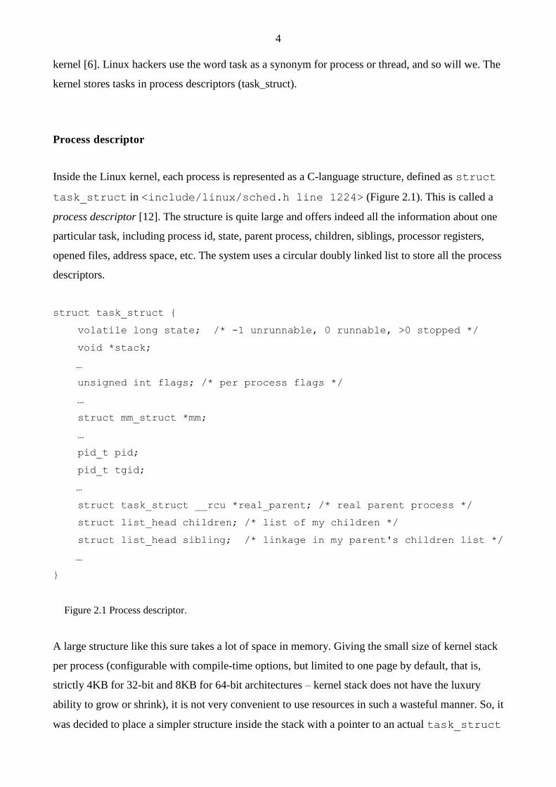
Inside the Linux kernel, each process is represented as a C-language structure, defined as struct
task_struct in <include/linux/sched.h line 1224> (Figure 2.1). This is called a
process descriptor [12]. The structure is quite large and offers indeed all the information about one
particular task, including process id, state, parent process, children, siblings, processor registers,
opened files, address space, etc. The system uses a circular doubly linked list to store all the process
descriptors.
struct task_struct {
volatile long state; /* -1 unrunnable, 0 runnable, >0 stopped */
void *stack;
…
unsigned int flags; /* per process flags */
…
struct mm_struct *mm;
…
pid_t pid;
pid_t tgid;
…
struct task_struct __rcu *real_parent; /* real parent process */
struct list_head children; /* list of my children */
struct list_head sibling; /* linkage in my parent's children list */
…
}
Figure 2.1 Process descriptor.
A large structure like this sure takes a lot of space in memory. Giving the small size of kernel stack
per process (configurable with compile-time options, but limited to one page by default, that is,
strictly 4KB for 32-bit and 8KB for 64-bit architectures – kernel stack does not have the luxury
ability to grow or shrink), it is not very convenient to use resources in such a wasteful manner. So, it
was decided to place a simpler structure inside the stack with a pointer to an actual task_struct
5
in it, namely struct thread_info. This rather tiny struct lives at the bottom of the kernel
stack of each process (if stacks grow down, or at the top of the stack, if stacks grow up) [1]. It is
strongly architecture dependent, how thread_info is presented; for x86 it is defined in
<arch/x86/include/asm/thread_info.h> and looks like this:
struct thread_info {
struct task_struct *task; /* main task structure */
struct exec_domain *exec_domain; /* execution domain */
__u32 flags; /* low level flags */
__u32 status; /* thread synchronous flags */
__u32 cpu; /* current CPU */
int saved_preempt_count;
mm_segment_t addr_limit;
struct restart_block restart_block;
void __user *sysenter_return;
unsigned int uaccess_err:1; /* uaccess failed */
};
To work with threads, we need to access their task_structs often, and even more often we need an
access to a currently running task. Looping through all available processes on the system would be
unwise and time consuming. That is why we have a macro named current. This macro has to be
implemented separately with every architecture for the reasons of variable size of stack or memory
page. Some architectures store a pointer to a currently running process in a register, others have to
calculate it every time, due to a very small amount of available registers. On x86, for example, we
do not have spare registers to waste [17], but luckily, we know where we can find thread_info,
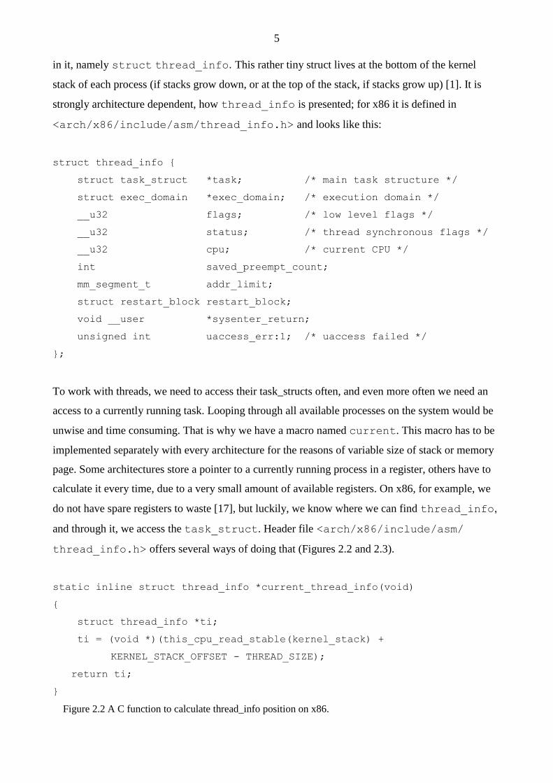
and through it, we access the task_struct. Header file <arch/x86/include/asm/
thread_info.h> offers several ways of doing that (Figures 2.2 and 2.3).
static inline struct thread_info *current_thread_info(void)
{
struct thread_info *ti;
ti = (void *)(this_cpu_read_stable(kernel_stack) +
KERNEL_STACK_OFFSET - THREAD_SIZE);
return ti;
}
Figure 2.2 A C function to calculate thread_info position on x86.
6
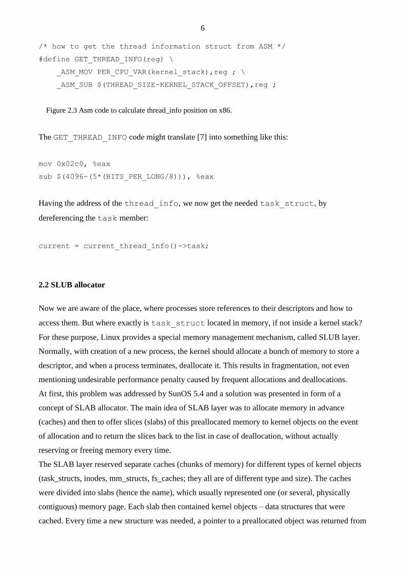
/* how to get the thread information struct from ASM */
#define GET_THREAD_INFO(reg) \
_ASM_MOV PER_CPU_VAR(kernel_stack),reg ; \
_ASM_SUB $(THREAD_SIZE-KERNEL_STACK_OFFSET),reg ;
Figure 2.3 Asm code to calculate thread_info position on x86.
The GET_THREAD_INFO code might translate [7] into something like this:
mov 0x02c0, %eax
sub $(4096-(5*(BITS_PER_LONG/8))), %eax
Having the address of the thread_info, we now get the needed task_struct, by
dereferencing the task member:
current = current_thread_info()->task;
2.2 SLUB allocator
Now we are aware of the place, where processes store references to their descriptors and how to
access them. But where exactly is task_struct located in memory, if not inside a kernel stack?
For these purpose, Linux provides a special memory management mechanism, called SLUB layer.
Normally, with creation of a new process, the kernel should allocate a bunch of memory to store a
descriptor, and when a process terminates, deallocate it. This results in fragmentation, not even
mentioning undesirable performance penalty caused by frequent allocations and deallocations.
At first, this problem was addressed by SunOS 5.4 and a solution was presented in form of a
concept of SLAB allocator. The main idea of SLAB layer was to allocate memory in advance
(caches) and then to offer slices (slabs) of this preallocated memory to kernel objects on the event
of allocation and to return the slices back to the list in case of deallocation, without actually
reserving or freeing memory every time.
The SLAB layer reserved separate caches (chunks of memory) for different types of kernel objects
(task_structs, inodes, mm_structs, fs_caches; they all are of different type and size). The caches
were divided into slabs (hence the name), which usually represented one (or several, physically
contiguous) memory page. Each slab then contained kernel objects – data structures that were
cached. Every time a new structure was needed, a pointer to a preallocated object was returned from
7
a cache. When an object was no longer needed, the kernel returned it back to the queue, thus
making a structure available again.
A slab could be in one of three states: empty, partially empty or full. Full meant that all the objects
were in use, so no allocation could be made. Empty slab, in contrast, had all its objects free. A
partial slab had some free objects and some of them used. On request, an object was to be returned
from a partial slab first, if one existed. Otherwise, an empty one was taken. If all the slabs were full,
a new one was spawned [12].
At the time the above approach was invented, it seemed like a good enhancement to the memory
management system in the kernel: no (or less) fragmentation, improved performance, more
intelligent allocation decisions due to fixed object sizes, no SMP locks with per-processor caches,
cache coloring. Kernel hackers tended not to wander into the SLAB code because it was, indeed,
complex and because, for the most part, it worked quite well.
The SLAB allocator has been at the core of Linux kernel's memory management for many years.
Over time, though, hardware evolved, computer systems grew bigger. The advantages of SLAB
allocator became its bottlenecks:
- SLAB layer maintained numerous queues of objects; these queues made allocations fast, but had
quite complicated implementation;
- the storage overhead was increasing drastically;
- each slab contained metadata, which was making alignment of objects harder;
- the code for cleaning up caches, when the system was out of memory, added another level of
complexity.
In his letter to Open Source Development Labs, Christoph Lameter [5] wrote:
“SLAB Object queues exist per node, per CPU. The alien cache queue even has a queue array
that contain a queue for each processor on each node. For very large systems the number of
queues and the number of objects that may be caught in those queues grows exponentially. On
our systems with 1k nodes / processors we have several gigabytes just tied up for storing
references to objects for those queues This does not include the objects that could be on those
queues. One fears that the whole memory of the machine could one day be consumed by those
queues.”
8
Author of the above lines presented his own allocator (SLUB), which fixed the many design flaws
SLAB had. SLUB promised better performance and scalability by dropping most of the queues and
related overhead by simplifying the SLAB structure in general. The current SLAB allocator
interface was retained. Metadata was removed from the blocks.
In SLUB allocator a slab is just a bunch of objects of a given size in a linked list. On request, a first
free object is found, removed from the list and returned to the caller.
Now, without any metadata in the slabs, the system has to know which of the memory pages of a
slab are free. This was done by staffing the relevant information into the system memory map – the
struct page, defined in <include/linux/mm_types.h>.
The new approach was taken well by the community and soon it was included in mainstream kernel
sources. Starting from kernel version 2.6.23, SLUB became the default allocator [11].
The code for both layers can be found in <mm/slab.c> and <mm/slub.c> accordingly.
2.3 Linked list
As mentioned above, Linux uses a circular doubly linked list to store all the processes on the system
and, as any big software project, Linux offers its own generic implementation of commonly used
data structures. Mainly to encourage code reuse instead of reinventing the wheel every time
someone needs to store a thing or two.
So, before we can go deeper into the topic of storing, managing and scheduling tasks, we might
want to take a look at the kernel’s way of implementing linked lists, which is indeed unique and
rather interesting approach to a simple data structure.
A normal doubly linked list is presented in Figure 2.4.
struct list_element {
void *data;
struct list_element *next; /* next element */
struct list_element *prev; /* previous element */
};
Figure 2.4 Simple doubly linked list.
Here the data is maintained by having a next and prev node pointers to the next and previous
elements of the list, accordingly. The Linux kernel approaches this in a different way: instead of
having a linked list structure, we embed a linked list node into a structure.
9
The code is declared in <include/linux/types.h>:
struct list_head {
struct list_head *next, *prev;
};
The next pointer points to the next element and the prev points to the previous element of the list.
What use do we have for a large amount of linked list nodes, you ask? The thing is how this
structure is used. A list_head is worthless by itself, thus it needs to be embedded into your own
structure:
struct task {
int num; /* number of the task to do */
bool is_awesome; /* is it something awesome? */
struct list_head mylist; /* the list of all tasks */
};
Naturally, the list has to be initialized before it can be used. The code for list initialization is located
inside <include/linux/list.h>:
#define LIST_HEAD_INIT(name) { &(name), &(name) }
#define LIST_HEAD(name) \
struct list_head name = LIST_HEAD_INIT(name)
static inline void INIT_LIST_HEAD(struct list_head *mylist)
{
list->next = mylist;
list->prev = mylist;
}
At runtime you do it like this:
struct task *some_task;
/* … allocate some_task… */
some_task->num = 1;
some_task->is_awesome = false;
10
INIT_LIST_HEAD(&some_task->mylist);
Initialize a list at compile time:
struct task some_task = {
.num = 1,
.is_awesome = false,
.list = LIST_HEAD_INIT(some_task.mylist),
};
To declare and initialize a static linked list directly, you can use
static LIST_HEAD(task_list);
The kernel provides a family of functions for manipulating linked lists (Figure 2.5). The functions
are inline C code and also located in <include/linux/list.h>. Not a surprise, they all are
O(1) in asymptotic complexity, which means that they execute in constant time regardless of the
amount of input. If we had 10 nodes or one million nodes in the list, adding or deleting would take
approximately the same time.
static inline void list_add(struct list_head *new,
struct list_head *head);
static inline void list_add_tail(struct list_head *new,
struct list_head *head);
static inline void list_del(struct list_head *entry);
Figure 2.5 Functions for linked list manipulation.
One major benefit of having a list is the ability to traverse the data stored in it. Linux kernel
provides a set of functions just for that. Going through all the elements in a list has naturally O(n)
complexity, where n is the number of nodes.
The most straightforward approach to traversing a list in the kernel would look like this:
struct list_head *h;
struct task *t;
list_for_each(h, &task_list) {
11
t = list_entry(h, struct task_list, mylist);
if (t->num == 1)
// do something
}
Here the function list_for_each iterates over each element of the list and the function
list_entry returns the structure that contains the list_head we are over at the moment.
There exists, though, a more elegant and simple way of traversing a list. A macro named
list_for_each_entry(pos, head, member)
includes the work, performed by list_entry(), making the iteration easier. This results in a
simple for loop: pos used as a loop cursor (iterating, until it hits starting point again), it is basically
what list_entry() returns, head is the head of the list we are iterating and member is a
list_head inside the struct.
The example with tasks would go like this:
struct task *t;
list_for_each_entry(t, task_list, list) {
if (t->num == 1)
break; /* or do something else */
}
The kernel also provides interfaces for iterating a list backwards, for removal of nodes during
iteration and many more ways of accessing and manipulating a linked list. All of these functions
and macros are defined in a header file <include/linux/list.h>.
2.4 Notes on C
volatile and const
The first line of the task_struct structure defines a variable to keep track of the execution state
of the process (definitions of the states can be found at the beginning of the header file
<include/linux/sched.h>). The variable is set as volatile, which is worth mentioning.
12
Volatile keyword is an ANSI C type modifier, which insures that the compiler does not use over-
optimization of putting certain variable into a register and, thus, creating a possibility for the
program code to use an old value, after the variable was updated. In other words, the compiler
generates code that reloads the variable from memory each time it is referenced by any of the
running threads, instead of just taking the value from a register (which would be a lot faster; this is
why it is called optimization).
For example, if two threads were to use the same variable to store an intermediate result of their
calculations, then one of them might just take an old value from a register without noticing that the
value has changed. Instead, the variable must be loaded from memory each time it is referenced.
Here the volatile keyword comes handy.
Using GNU Compiler Collection, also known as gcc, one has to apply the -O2 option (which is the
default in most cases of compiling the kernel), or higher, to see the effect of over-optimization.
With lesser or none at all optimizations, the compiler is likely to reload registers every time any
variable is referenced.
The usage of volatile keyword is particularly important in the case of process’s state. Because the
kernel often needs to change states of processes from different places, it will be very unhappy if, for
example, two processes were set RUNNABLE at the same time on a single CPU hardware.
Another C language type modifier that is mostly ignored by beginner programmers and often
misunderstood even by professionals is const. This keyword should not be interpreted as “constant”,
instead it should be taken as “read-only”. For example,
const int *iptr;
is a pointer to a read-only integer. Herewith, a pointer can be changed, but an integer cannot. On the
other hand,
int * const iptr;
is a constant pointer to an integer, where an int can be changed, but a pointer cannot be put to
point elsewhere.
It is a good practice to declare parameters of functions read-only, if we have no intentions of
changing them:
13
static inline void prefetch(const void *x)
{
__asm ___volatile__ ("debt 0,%0" : : "r" (x) );
}
The two keywords can be used together, say, to declare a constant pointer to a volatile hardware
register:
uint8_t volatile * const p_irq_reg = (uint8_t *) 0x80000;
Branch prediction hints
In Linux kernel code, one often finds calls to likely() and unlikely() in conditions like:
struct sched_entity *curr = cfs_rq->curr;
if (unlikely(!curr))
return;
These macros are hints for the compiler that allow it to optimize the if-statement by knowing which
branch is the likeliest one [12]. If the compiler has this prediction information, it can generate the
most optimal assembly code around the branch. The definition of the macros is found in
<include/linux/compiler.h> and, through some pretty scary #defines, boils down to this:
#define likely(x) __builtin_expect(!!(x), 1)
#define unlikely(x) __builtin_expect(!!(x), 0)
The __builtin_expect() directive optimizes things by ordering the generated assembly code
correctly, to optimize the usage of the processor pipeline. To do so, it arranges the code so that the
likeliest branch is executed without performing any jmp instruction (which has the bad effect of
flushing the processor pipeline) [17].
The !!(x) syntax is used here, because there is no boolean type in C programming language, but,
according to the standard [8], operators like “==“, “&&” or “!” should return 0 for false and 1 for
true. So, if you have
int x = 3;
14
you can force it into a “boolean” value by negating:
/*
* will always return 0 (as false)
*/
x = !x
/*
* assuming starting position, where x = 3,
* this will always return 1 (for true)
*/
x = !!(x)
15
3. Scheduling
Linux is a multitasking operating system. This basically means that the system can execute multiple
processes simultaneously, giving the illusion of running only one process, a user is focused on, at
any given moment of time. On single processor(core) systems this is true, only one process can be
executing at any given moment of time, faking concurrency. Multiprocessor hardware (or multicore
processor), however, allows tasks to run actually in parallel. On either type of machine, there are
still many processes in memory that are not executing, but waiting to run or sleeping. The part of
the kernel, which is responsible for granting CPU time to tasks, is called process scheduler.
A scheduler chooses the next task to be run, and maintains the order, which all the processes on the
system should be run in, as well. In the same way as most operating systems out there, Linux
implements preemptive multitasking. Meaning, the scheduler decides when one process ceases
running and the other begins. The act of involuntarily suspending a running process is called
preemption [15]. Preemptions are caused by timer interrupts. A timer interrupt is basically a clock
tick inside the kernel, the clock ticks 1000 times a second; this will be covered in greater details
later in the chapter. When an interrupt happens, scheduler has to decide whether to grant CPU to
some other process and, if so, to which one. The amount of time a process gets to run is called
timeslice of a process.
Tasks are usually separated into interactive (also called I/O bound) and non-interactive (processor
bound or “batch processes”) ones [6]. Interactive tasks are hugely dependent on input/output
operations (for example, graphical user interfaces) and tend not to always use their timeslices fully,
giving up the processor to other tasks. Conversely, non-interactive processes (e.g., some
mathematical calculations) tend to use CPU heavily. They usually run until preempted, using all of
their timeslices, because they do not block on I/O requests very often.
Although such classifications exist, they are not mutually exclusive. Any given process can belong
to both groups. A text editor, for example, is waiting for user input most of the time, but can easily
put CPU under a heavy load with spell checking.
A scheduling policy in the system has to balance between the two types of processes, and to make
sure that every task gets enough execution resources, with no visible effect on the performance of
other jobs. To maximize CPU utilization and to guarantee fast response times, Linux tends to
provide non-interactive processes with longer “uninterrupted” slices in a row, but to run them less
frequently. I/O bound tasks, in turn, possess the processor more often, but for shorter periods of
time.
16
3.1 Structure
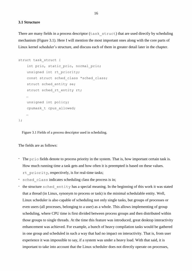
There are many fields in a process descriptor (task_struct) that are used directly by scheduling
mechanism (Figure 3.1). Here I will mention the most important ones along with the core parts of
Linux kernel scheduler’s structure, and discuss each of them in greater detail later in the chapter.
struct task_struct {
int prio, static_prio, normal_prio;
unsigned int rt_priority;
const struct sched_class *sched_class;
struct sched_entity se;
struct sched_rt_entity rt;
…
unsigned int policy;
cpumask_t cpus_allowed;
…
};
Figure 3.1 Fields of a process descriptor used in scheduling.
The fields are as follows:
- The prio fields denote to process priority in the system. That is, how important certain task is.
How much running time a task gets and how often it is preempted is based on these values.
rt_priority, respectively, is for real-time tasks;
- sched_class indicates scheduling class the process is in;
- the structure sched_entity has a special meaning. In the beginning of this work it was stated
that a thread (in Linux, synonym to process or task) is the minimal schedulable entity. Well,
Linux scheduler is also capable of scheduling not only single tasks, but groups of processes or
even users (all processes, belonging to a user) as a whole. This allows implementing of group
scheduling, where CPU time is first divided between process groups and then distributed within
those groups to single threads. At the time this feature was introduced, great desktop interactivity
enhancement was achieved. For example, a bunch of heavy compilation tasks would be gathered
in one group and scheduled in such a way that had no impact on interactivity. That is, from user
experience it was impossible to say, if a system was under a heavy load. With that said, it is
important to take into account that the Linux scheduler does not directly operate on processes,
17
but works with schedulable entities. Such an entity is represented by struct
sched_entity. Note, that it is not a pointer; the structure is embedded into the process
descriptor. In this work, we concentrate only on the simplest case of a per-process scheduling.
Since the scheduler is designed to work with entities, it sees even single processes as such
entities and, therefore, uses the mentioned structure to operate on them. sched_rt_entity
denotes to an entity, scheduled with real-time preferences.
- policy holds the scheduling policy of a task: basically means special scheduling decisions for
some particular group of processes (longer timeslices, higher priorities, etc.). Current Linux
kernel version supports five types of policies:
SCHED_NORMAL: the scheduling policy that is used for regular tasks;
SCHED_BATCH: does not preempt nearly as often as regular tasks would, thereby allowing
tasks to run longer and make better use of caches but at the cost of interactivity. This is well
suited for batch jobs (CPU-intensive batch processes that are not interactive);
SCHED_IDLE: this is even weaker than nice 19 (means a very low priority; process
priorities are discussed later in this chapter), but it is not a true idle task. Some background
system threads obey this policy, mainly not to disturb normal way of things;
SCHED_FIFO and SCHED_RR are for soft real-time processes. Handled by real-time
scheduler in <kernel/sched/rt.c> and specified by POSIX standard. RR implements
round robin method, while SCHED_FIFO uses first in first out queuing mechanism.
- cpus_allowed is a type-struct, containing bit field, which indicates a task’s affinity —
binding to a particular set of CPU core(s) [15]. Can be set from user-space by using the
sched_setaffinity system call.
In the follow up sections I will go through all the mentioned fundamental pieces that indicate task
state and behavior, thus overviewing the core part of the Linux process scheduler.
18
Priorities
Process priority
All UNIX based operating systems, and Linux is not an exception, implement a priority based
scheduling. The main idea is to assign some value to every task in the system, and then determine
how important a task is by looking at this value and comparing it to other tasks’ values. If two
processes happen to have the same value, run them one after another repeatedly. A process with
higher value runs before those with lower value; it would also be fair to assign longer execution
time to a task with higher value.
As mentioned above, Linux does implement scheduling, based on priorities of processes, only not
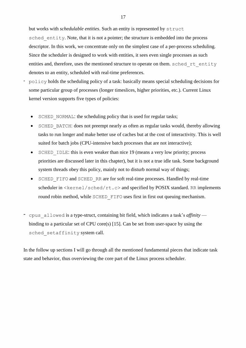
in such a simple way. Each task is assigned a nice value, which is an integer from -20 to 19 with
default being 0.
<— higher priority
-20_ _ _ _ _ 0 _ _ _ _ _+19
Figure 3.2 Nice priority scale.
The higher niceness, the lower the priority of a task — it is “nice” to others (Figure 3.2). Probably,
in every UNIX system you can print a list of processes and see their niceness from a command
shell, for example,
$ ps -Al (lowercase L)
in Linux shows all processes with nice (NI column) values.
The kernel uses a system call nice(int increment) to change current process’s priority [13].
The syscall and related code can be found in <kernel/sched/core.c>.
Not only kernel is in charge of prioritizing tasks, it is possible to alter process priorities from user
space too. You can either start a new program along with setting a nice value:
$ nice -n increment utility
“increment” can be a negative or positive integer (added to default of 0); or change the value of an
already running task:
19
$ renice -n priority -p PID
By default, however, a user can only increase niceness (lower priority) and of only the processes
(s)he has started. To increase priority or to alter another user’s process, one must be root.
All of the above is true for “normal” processes with no specific constraints on execution time. Some
tasks are just more important than the others, so, some of them run longer and do not wait in the
queue as much as others. Most Linux users should be familiar with process priorities as they are. In
addition to these, however, there exists “the other kind” of tasks in the system. Namely – real-time,
or rt, processes. The reason why a basic OS user might not be aware of such special kind of tasks is
that users with their desktop (or even server) computers do not usually need the kind of seriousness
in their everyday work that rt offers.
Real-time tasks are the ones that guarantee their execution inside some strict time boundaries (we
are going to cover the topic of scheduling rt processes in a separate chapter towards the end). There
are two kinds of real-time processes [9]:
- Hard real-time processes. Bound by strict time limits, in which a task must be completed. A
good example would be a flying helicopter. The machine has to react to the movements of cyclic
control stick within certain amount of time, so the pilot could maneuver. Besides that, the
reaction has to come somewhat in the same time frame and, in general, act predictably every time
it is expected to happen, even when unlikely or adverse conditions prevail. Note, that this does
not imply that a time frame should be short. Instead, it is important that the frame is never
exceeded. One could not stress enough the significance of a hard real-time process not missing
its deadline.
Linux does not support hard real time processing by itself. There are modifications, though, such
as RTLinux (they are often called RTOS: Real Time Operating Systems). Systems like that run
the entire Linux kernel in a separate fully preemptive process; rt tasks just do whatever needs
done when it has to be done, regardless of what Linux is doing at any point in time.
- Soft real-time processes. These are a “softer version” of hard real-time processes. Although there
are boundaries, nothing dramatic should happen, if a task runs a bit late. In practice, soft rt
processes (kind of) guarantee the time frame, but you should not make your (or anyone else’s)
life depend on it. As an example, a CD burning software would work. Packets of data must be
received to a writer at certain rate, because data is written to a CD as a stream with certain speed.
If the system is under high load, a packet might come late, which would result in a broken
medium. Not as dramatic, as a crashing helicopter, is it? Also VOIP software programs use
protocols with soft real-time guarantees to deliver sound and video signal over the network; we
20
all know how well they are doing. Nonetheless, a real-time process will always get a higher
priority in the system than any “normal” process.
Priorities of real-time processes in a Linux system range from 0 to 99. Unlike nice values, here
“more” also means “more” — greater number indicates higher priority (Figure 3.3).
As we already know, any real-time process is far more important than any “normal” user-land task.
So, rt priories lay separately from nice values; any task with the lowest rt priority is considered by
the system as more significant than any task with the lowest nice value.
higher priority —>
0_ _ _ _ _ _ _ _ _ _ _ _ _ _ _ _ _ _99
Figure 3.3 Real-time priority scale.
Linux kernel, like any other modern UNIX system, implements real-time priorities according to
“Real-time Extensions” of POSIX 1b standard [20]. You can see the rt tasks running on the system
using the following commands:
$ ps -eo pid, rtprio, cmd
(in the output, RTPRIO column shows the rt priority, the hyphen means that the task is not rt) or,
per process:
$ chrt -p pid
You can also alter the real-time priority of a task on Linux with
# chrt -p prio pid
Note, if you are dealing with a system process (usually you do not want to make user processes rt),
you have to be root to change its real-time priority.
21
Process priority (kernel’s perspective)
Up to this point we have examined priorities of processes from a user-space point of view. As you
may guess, the in-kernel reality is not so simple. Actually, the kernel sees priorities in quite a
different way than a user, and a lot more effort is put to calculate and manage them [15].
User-space calls nice to assign a value between -20 and +19 to a process, which in turn executes
nice system call (there is also an alternative syscall for setting niceness – setpriority(int
which, int who, int prio) for altering priorities of individual tasks, process groups or
even all user’s tasks – which, who is related to which and means an ID of a task, a group of tasks
or a user, and prio indicates niceness) [13]. Lower number means higher priority. For basic
“normal” processes, this is it.
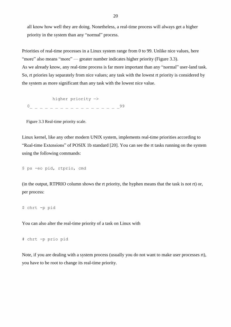
The kernel, in turn, uses a scale from 0 to 139 to represent priorities internally. Again, inverted,
lower value indicates higher priority. Numbers from 0 to 99 are reserved for real-time processes and
100 to 139 (mapped to nice -20 – +19) are for normal processes (Figure 3.4).
<— higher priority
0_ _ _ _ _ _ _ _ _ _ _ _ _ _ _ _ _ _99_100_ _ _ _ _ _ _ _ _ _ _139
real-time normal
Figure 3.4 Kernel priority scale.
Internal kernel representation of process priority scale and macros for mapping user-space to
kernel-space priority values can be found in <include/linux/sched/prio.h> header file:
#define MAX_NICE 19
#define MIN_NICE -20
#define NICE_WIDTH (MAX_NICE - MIN_NICE + 1)
…
#define MAX_USER_RT_PRIO 100
#define MAX_RT_PRIO MAX_USER_RT_PRIO
#define MAX_PRIO (MAX_RT_PRIO + NICE_WIDTH)
#define DEFAULT_PRIO (MAX_RT_PRIO + NICE_WIDTH / 2)
22
/*
* Convert user-nice values [ -20 ... 0 ... 19 ]
* to static priority [ MAX_RT_PRIO..MAX_PRIO-1 ],
* and back.
*/
#define NICE_TO_PRIO(nice) ((nice) + DEFAULT_PRIO)
#define PRIO_TO_NICE(prio) ((prio) - DEFAULT_PRIO)
/*
* 'User priority' is the nice value converted to something we
* can work with better when scaling various scheduler parameters,
* it's a [ 0 ... 39 ] range.
*/
#define USER_PRIO(p) ((p)-MAX_RT_PRIO)
#define TASK_USER_PRIO(p) USER_PRIO((p)->static_prio)
#define MAX_USER_PRIO (USER_PRIO(MAX_PRIO))
Calculating priorities
Inside task_struct, there are several fields representing process priority. Namely:
int prio, static_prio, normal_prio;
unsigned int rt_priority;
They all are related to each other. Let us examine, how.
static_prio is the priority, given “statically” by a user (and mapped into kernel’s
representation) or by the system itself:
p->static_prio = NICE_TO_PRIO(nice_value);
normal_priority holds the one based on static_prio and scheduling policy of a process, that is,
whether a task is real-time or “normal” process. Tasks with the same static priority that belong to
different policies will get different normal priorities. Child processes inherit the normal priorities
from their parent processes when forked.
23
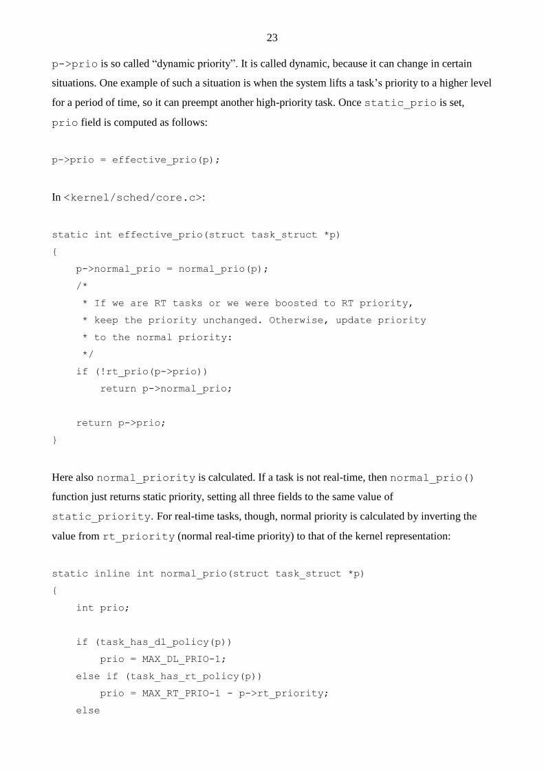
p->prio is so called “dynamic priority”. It is called dynamic, because it can change in certain
situations. One example of such a situation is when the system lifts a task’s priority to a higher level
for a period of time, so it can preempt another high-priority task. Once static_prio is set,
prio field is computed as follows:
p->prio = effective_prio(p);
In <kernel/sched/core.c>:
static int effective_prio(struct task_struct *p)
{
p->normal_prio = normal_prio(p);
/*
* If we are RT tasks or we were boosted to RT priority,
* keep the priority unchanged. Otherwise, update priority
* to the normal priority:
*/
if (!rt_prio(p->prio))
return p->normal_prio;
return p->prio;
}
Here also normal_priority is calculated. If a task is not real-time, then normal_prio()
function just returns static priority, setting all three fields to the same value of
static_priority. For real-time tasks, though, normal priority is calculated by inverting the
value from rt_priority (normal real-time priority) to that of the kernel representation:
static inline int normal_prio(struct task_struct *p)
{
int prio;
if (task_has_dl_policy(p))
prio = MAX_DL_PRIO-1;
else if (task_has_rt_policy(p))
prio = MAX_RT_PRIO-1 - p->rt_priority;
else
24
prio = __normal_prio(p);
return prio;
}
static inline int __normal_prio(struct task_struct *p)
{
return p->static_prio;
}
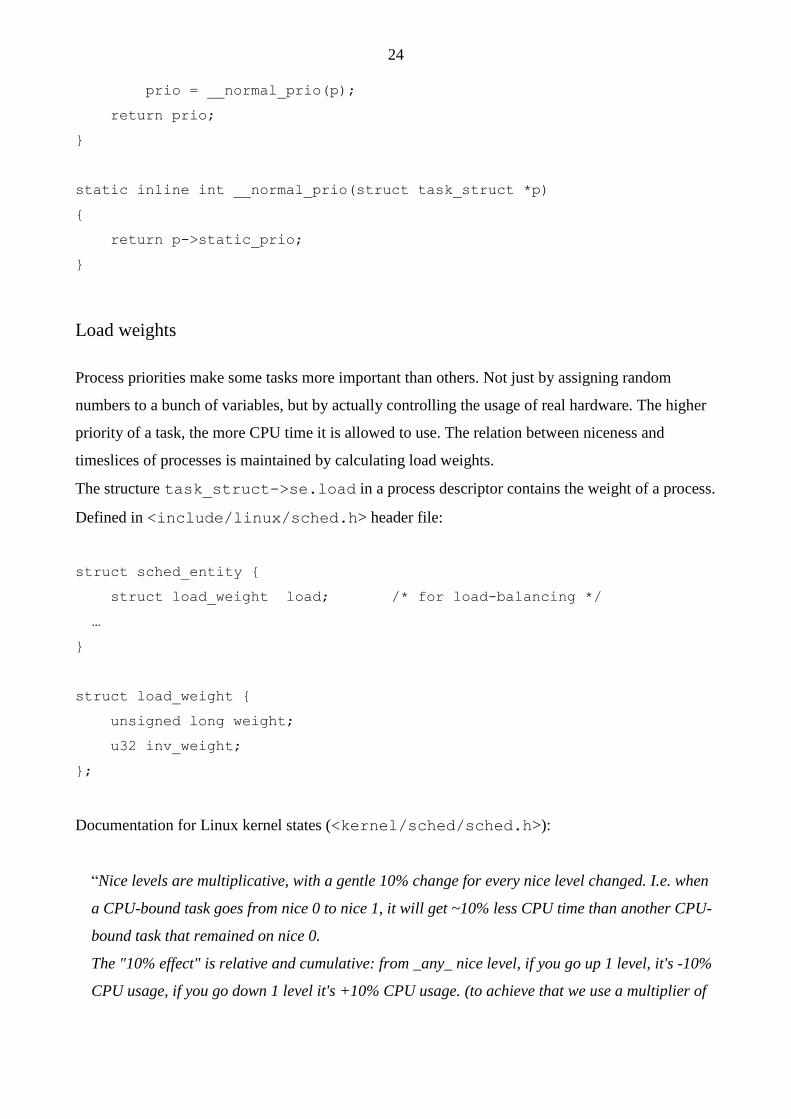
Load weights
Process priorities make some tasks more important than others. Not just by assigning random
numbers to a bunch of variables, but by actually controlling the usage of real hardware. The higher
priority of a task, the more CPU time it is allowed to use. The relation between niceness and
timeslices of processes is maintained by calculating load weights.
The structure task_struct->se.load in a process descriptor contains the weight of a process.
Defined in <include/linux/sched.h> header file:
struct sched_entity {
struct load_weight load; /* for load-balancing */
…
}
struct load_weight {
unsigned long weight;
u32 inv_weight;
};
Documentation for Linux kernel states (<kernel/sched/sched.h>):
“Nice levels are multiplicative, with a gentle 10% change for every nice level changed. I.e. when
a CPU-bound task goes from nice 0 to nice 1, it will get ~10% less CPU time than another CPU-
bound task that remained on nice 0.
The "10% effect" is relative and cumulative: from _any_ nice level, if you go up 1 level, it's -10%
CPU usage, if you go down 1 level it's +10% CPU usage. (to achieve that we use a multiplier of
25
1.25. If a task goes up by ~10% and another task goes down by ~10% then the relative distance
between them is ~25%.)”.
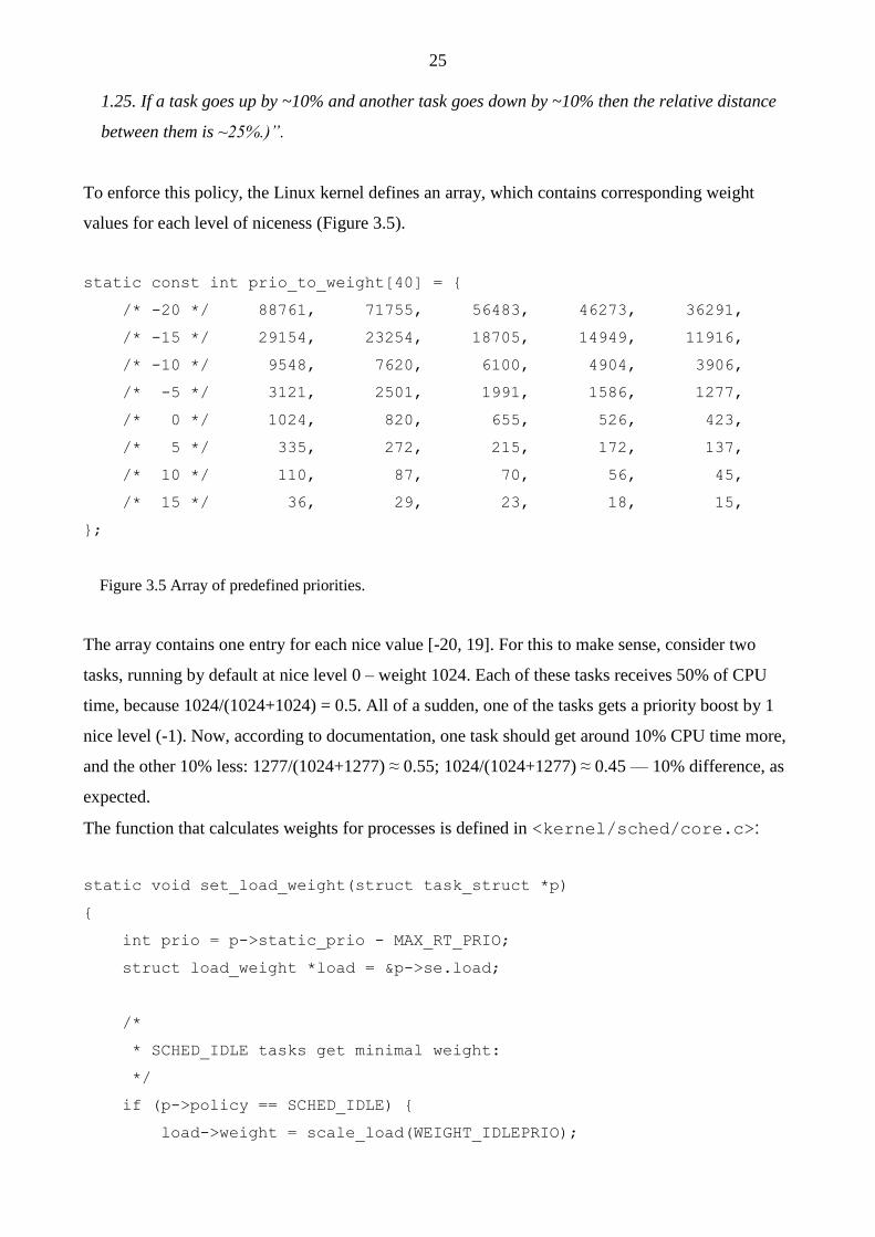
To enforce this policy, the Linux kernel defines an array, which contains corresponding weight
values for each level of niceness (Figure 3.5).
static const int prio_to_weight[40] = {
/* -20 */ 88761, 71755, 56483, 46273, 36291,
/* -15 */ 29154, 23254, 18705, 14949, 11916,
/* -10 */ 9548, 7620, 6100, 4904, 3906,
/* -5 */ 3121, 2501, 1991, 1586, 1277,
/* 0 */ 1024, 820, 655, 526, 423,
/* 5 */ 335, 272, 215, 172, 137,
/* 10 */ 110, 87, 70, 56, 45,
/* 15 */ 36, 29, 23, 18, 15,
};
Figure 3.5 Array of predefined priorities.
The array contains one entry for each nice value [-20, 19]. For this to make sense, consider two
tasks, running by default at nice level 0 – weight 1024. Each of these tasks receives 50% of CPU
time, because 1024/(1024+1024) = 0.5. All of a sudden, one of the tasks gets a priority boost by 1
nice level (-1). Now, according to documentation, one task should get around 10% CPU time more,
and the other 10% less: 1277/(1024+1277) ≈ 0.55; 1024/(1024+1277) ≈ 0.45 — 10% difference, as
expected.
The function that calculates weights for processes is defined in <kernel/sched/core.c>:
static void set_load_weight(struct task_struct *p)
{
int prio = p->static_prio - MAX_RT_PRIO;
struct load_weight *load = &p->se.load;
/*
* SCHED_IDLE tasks get minimal weight:
*/
if (p->policy == SCHED_IDLE) {
load->weight = scale_load(WEIGHT_IDLEPRIO);
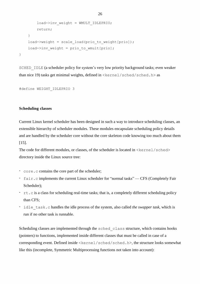
26
load->inv_weight = WMULT_IDLEPRIO;
return;
}
load->weight = scale_load(prio_to_weight[prio]);
load->inv_weight = prio_to_wmult[prio];
}
SCHED_IDLE (a scheduler policy for system’s very low priority background tasks; even weaker
than nice 19) tasks get minimal weights, defined in <kernel/sched/sched.h> as
#define WEIGHT_IDLEPRIO 3
Scheduling classes
Current Linux kernel scheduler has been designed in such a way to introduce scheduling classes, an
extensible hierarchy of scheduler modules. These modules encapsulate scheduling policy details
and are handled by the scheduler core without the core skeleton code knowing too much about them
[15].
The code for different modules, or classes, of the scheduler is located in <kernel/sched>
directory inside the Linux source tree:
- core.c contains the core part of the scheduler;
- fair.c implements the current Linux scheduler for “normal tasks” — CFS (Completely Fair
Scheduler);
- rt.c is a class for scheduling real-time tasks; that is, a completely different scheduling policy
than CFS;
- idle_task.c handles the idle process of the system, also called the swapper task, which is
run if no other task is runnable.
Scheduling classes are implemented through the sched_class structure, which contains hooks
(pointers) to functions, implemented inside different classes that must be called in case of a
corresponding event. Defined inside <kernel/sched/sched.h>, the structure looks somewhat
like this (incomplete, Symmetric Multiprocessing functions not taken into account):
27
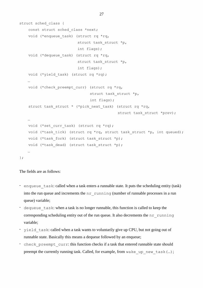
struct sched_class {
const struct sched_class *next;
void (*enqueue_task) (struct rq *rq,
struct task_struct *p,
int flags);
void (*dequeue_task) (struct rq *rq,
struct task_struct *p,
int flags);
void (*yield_task) (struct rq *rq);
…
void (*check_preempt_curr) (struct rq *rq,
struct task_struct *p,
int flags);
struct task_struct * (*pick_next_task) (struct rq *rq,
struct task_struct *prev);
…
void (*set_curr_task) (struct rq *rq);
void (*task_tick) (struct rq *rq, struct task_struct *p, int queued);
void (*task_fork) (struct task_struct *p);
void (*task_dead) (struct task_struct *p);
…
};
The fields are as follows:
- enqueue_task: called when a task enters a runnable state. It puts the scheduling entity (task)
into the run queue and increments the nr_running (number of runnable processes in a run
queue) variable;
- dequeue_task: when a task is no longer runnable, this function is called to keep the
corresponding scheduling entity out of the run queue. It also decrements the nr_running
variable;
- yield_task: called when a task wants to voluntarily give up CPU, but not going out of
runnable state. Basically this means a dequeue followed by an enqueue;
- check_preempt_curr: this function checks if a task that entered runnable state should
preempt the currently running task. Called, for example, from wake_up_new_task(…);
28
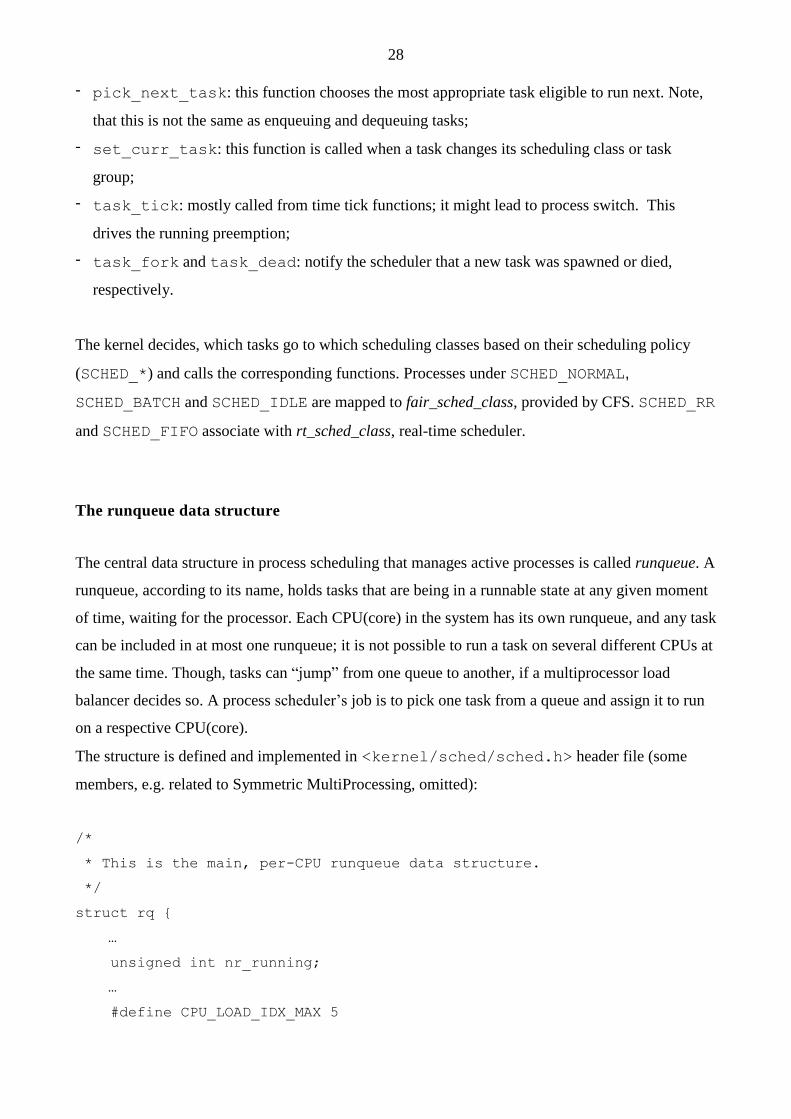
- pick_next_task: this function chooses the most appropriate task eligible to run next. Note,
that this is not the same as enqueuing and dequeuing tasks;
- set_curr_task: this function is called when a task changes its scheduling class or task
group;
- task_tick: mostly called from time tick functions; it might lead to process switch. This
drives the running preemption;
- task_fork and task_dead: notify the scheduler that a new task was spawned or died,
respectively.
The kernel decides, which tasks go to which scheduling classes based on their scheduling policy
(SCHED_*) and calls the corresponding functions. Processes under SCHED_NORMAL,
SCHED_BATCH and SCHED_IDLE are mapped to fair_sched_class, provided by CFS. SCHED_RR
and SCHED_FIFO associate with rt_sched_class, real-time scheduler.
The runqueue data structure
The central data structure in process scheduling that manages active processes is called runqueue. A
runqueue, according to its name, holds tasks that are being in a runnable state at any given moment
of time, waiting for the processor. Each CPU(core) in the system has its own runqueue, and any task
can be included in at most one runqueue; it is not possible to run a task on several different CPUs at
the same time. Though, tasks can “jump” from one queue to another, if a multiprocessor load
balancer decides so. A process scheduler’s job is to pick one task from a queue and assign it to run
on a respective CPU(core).
The structure is defined and implemented in <kernel/sched/sched.h> header file (some
members, e.g. related to Symmetric MultiProcessing, omitted):
/*
* This is the main, per-CPU runqueue data structure.
*/
struct rq {
…
unsigned int nr_running;
…
#define CPU_LOAD_IDX_MAX 5
29
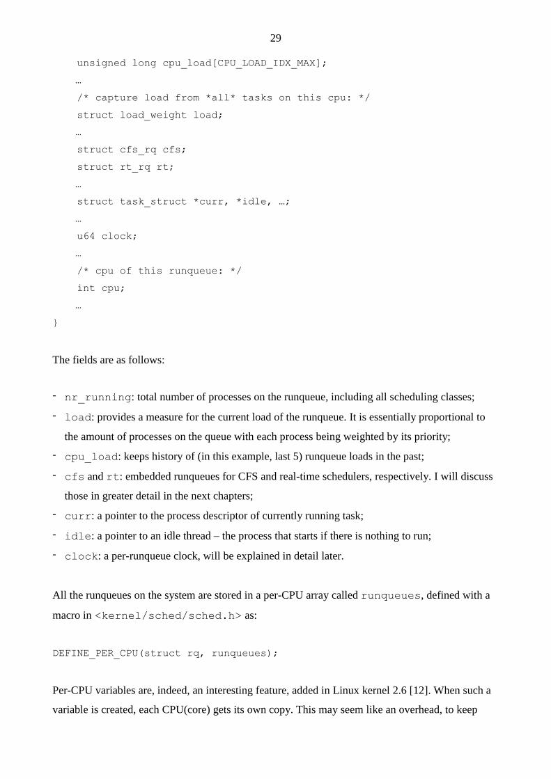
unsigned long cpu_load[CPU_LOAD_IDX_MAX];
…
/* capture load from *all* tasks on this cpu: */
struct load_weight load;
…
struct cfs_rq cfs;
struct rt_rq rt;
…
struct task_struct *curr, *idle, …;
…
u64 clock;
…
/* cpu of this runqueue: */
int cpu;
…
}
The fields are as follows:
- nr_running: total number of processes on the runqueue, including all scheduling classes;
- load: provides a measure for the current load of the runqueue. It is essentially proportional to
the amount of processes on the queue with each process being weighted by its priority;
- cpu_load: keeps history of (in this example, last 5) runqueue loads in the past;
- cfs and rt: embedded runqueues for CFS and real-time schedulers, respectively. I will discuss
those in greater detail in the next chapters;
- curr: a pointer to the process descriptor of currently running task;
- idle: a pointer to an idle thread – the process that starts if there is nothing to run;
- clock: a per-runqueue clock, will be explained in detail later.
All the runqueues on the system are stored in a per-CPU array called runqueues, defined with a
macro in <kernel/sched/sched.h> as:
DEFINE_PER_CPU(struct rq, runqueues);
Per-CPU variables are, indeed, an interesting feature, added in Linux kernel 2.6 [12]. When such a
variable is created, each CPU(core) gets its own copy. This may seem like an overhead, to keep
30
several instances of the same thing, especially in such a resource-tight place as an operating
system’s kernel, but there are great advantages. Access to a per-CPU variable requires almost no
locking, because the variable is not shared, and thus, the chances to end up with race conditions are
minimal. The kernel can also keep such variables in their respective processors' caches, which leads
to a significant performance boost for frequently accessed quantities.
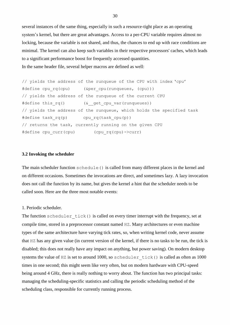
In the same header file, several helper macros are defined as well:
// yields the address of the runqueue of the CPU with index ‘cpu’
#define cpu_rq(cpu) (&per_cpu(runqueues, (cpu)))
// yields the address of the runqueue of the current CPU
#define this_rq() (&__get_cpu_var(runqueues))
// yields the address of the runqueue, which holds the specified task
#define task_rq(p) cpu_rq(task_cpu(p))
// returns the task, currently running on the given CPU
#define cpu_curr(cpu) (cpu_rq(cpu)->curr)
3.2 Invoking the scheduler
The main scheduler function schedule() is called from many different places in the kernel and
on different occasions. Sometimes the invocations are direct, and sometimes lazy. A lazy invocation
does not call the function by its name, but gives the kernel a hint that the scheduler needs to be
called soon. Here are the three most notable events:
1. Periodic scheduler.
The function scheduler_tick() is called on every timer interrupt with the frequency, set at
compile time, stored in a preprocessor constant named HZ. Many architectures or even machine
types of the same architecture have varying tick rates, so, when writing kernel code, never assume
that HZ has any given value (in current version of the kernel, if there is no tasks to be run, the tick is
disabled; this does not really have any impact on anything, but power saving). On modern desktop
systems the value of HZ is set to around 1000, so scheduler_tick() is called as often as 1000
times in one second; this might seem like very often, but on modern hardware with CPU-speed
being around 4 GHz, there is really nothing to worry about. The function has two principal tasks:
managing the scheduling-specific statistics and calling the periodic scheduling method of the
scheduling class, responsible for currently running process.
31
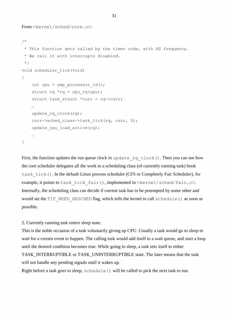
From <kernel/sched/core.c>:
/*
* This function gets called by the timer code, with HZ frequency.
* We call it with interrupts disabled.
*/
void scheduler_tick(void)
{
int cpu = smp_processor_id();
struct rq *rq = cpu_rq(cpu);
struct task_struct *curr = rq->curr;
…
update_rq_clock(rq);
curr->sched_class->task_tick(rq, curr, 0);
update_cpu_load_active(rq);
…
}
First, the function updates the run queue clock in update_rq_clock(). Then you can see how
the core scheduler delegates all the work to a scheduling class (of currently running task) hook
task_tick(). In the default Linux process scheduler (CFS or Completely Fair Scheduler), for
example, it points to task_tick_fair(), implemented in <kernel/sched/fair.c>.
Internally, the scheduling class can decide if current task has to be preempted by some other and
would set the TIF_NEED_RESCHED flag, which tells the kernel to call schedule() as soon as
possible.
2. Currently running task enters sleep state.
This is the noble occasion of a task voluntarily giving up CPU. Usually a task would go to sleep to
wait for a certain event to happen. The calling task would add itself to a wait queue, and start a loop
until the desired condition becomes true. While going to sleep, a task sets itself to either
TASK_INTERRUPTIBLE or TASK_UNINTERRUPTIBLE state. The later means that the task
will not handle any pending signals until it wakes up.
Right before a task goes to sleep, schedule() will be called to pick the next task to run.
32
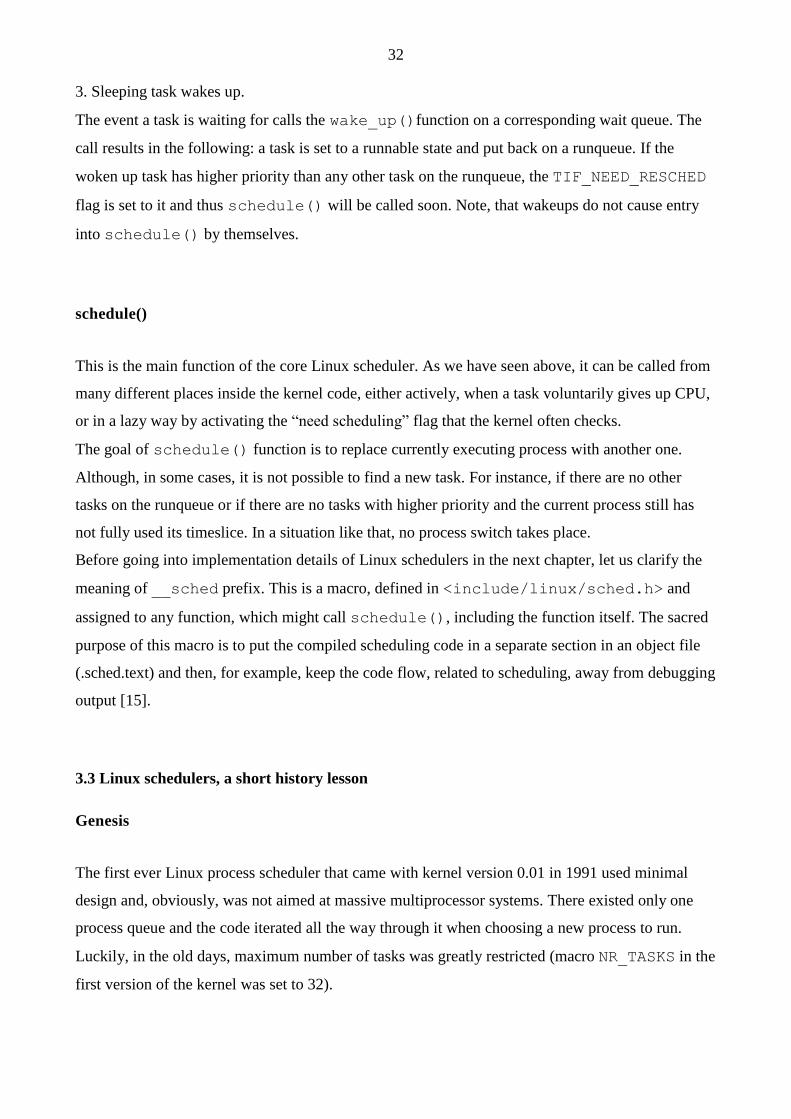
3. Sleeping task wakes up.
The event a task is waiting for calls the wake_up()function on a corresponding wait queue. The
call results in the following: a task is set to a runnable state and put back on a runqueue. If the
woken up task has higher priority than any other task on the runqueue, the TIF_NEED_RESCHED
flag is set to it and thus schedule() will be called soon. Note, that wakeups do not cause entry
into schedule() by themselves.
schedule()
This is the main function of the core Linux scheduler. As we have seen above, it can be called from
many different places inside the kernel code, either actively, when a task voluntarily gives up CPU,
or in a lazy way by activating the “need scheduling” flag that the kernel often checks.
The goal of schedule() function is to replace currently executing process with another one.
Although, in some cases, it is not possible to find a new task. For instance, if there are no other
tasks on the runqueue or if there are no tasks with higher priority and the current process still has
not fully used its timeslice. In a situation like that, no process switch takes place.
Before going into implementation details of Linux schedulers in the next chapter, let us clarify the
meaning of __sched prefix. This is a macro, defined in <include/linux/sched.h> and
assigned to any function, which might call schedule(), including the function itself. The sacred
purpose of this macro is to put the compiled scheduling code in a separate section in an object file
(.sched.text) and then, for example, keep the code flow, related to scheduling, away from debugging
output [15].
3.3 Linux schedulers, a short history lesson
Genesis
The first ever Linux process scheduler that came with kernel version 0.01 in 1991 used minimal
design and, obviously, was not aimed at massive multiprocessor systems. There existed only one
process queue and the code iterated all the way through it when choosing a new process to run.
Luckily, in the old days, maximum number of tasks was greatly restricted (macro NR_TASKS in the
first version of the kernel was set to 32).
33
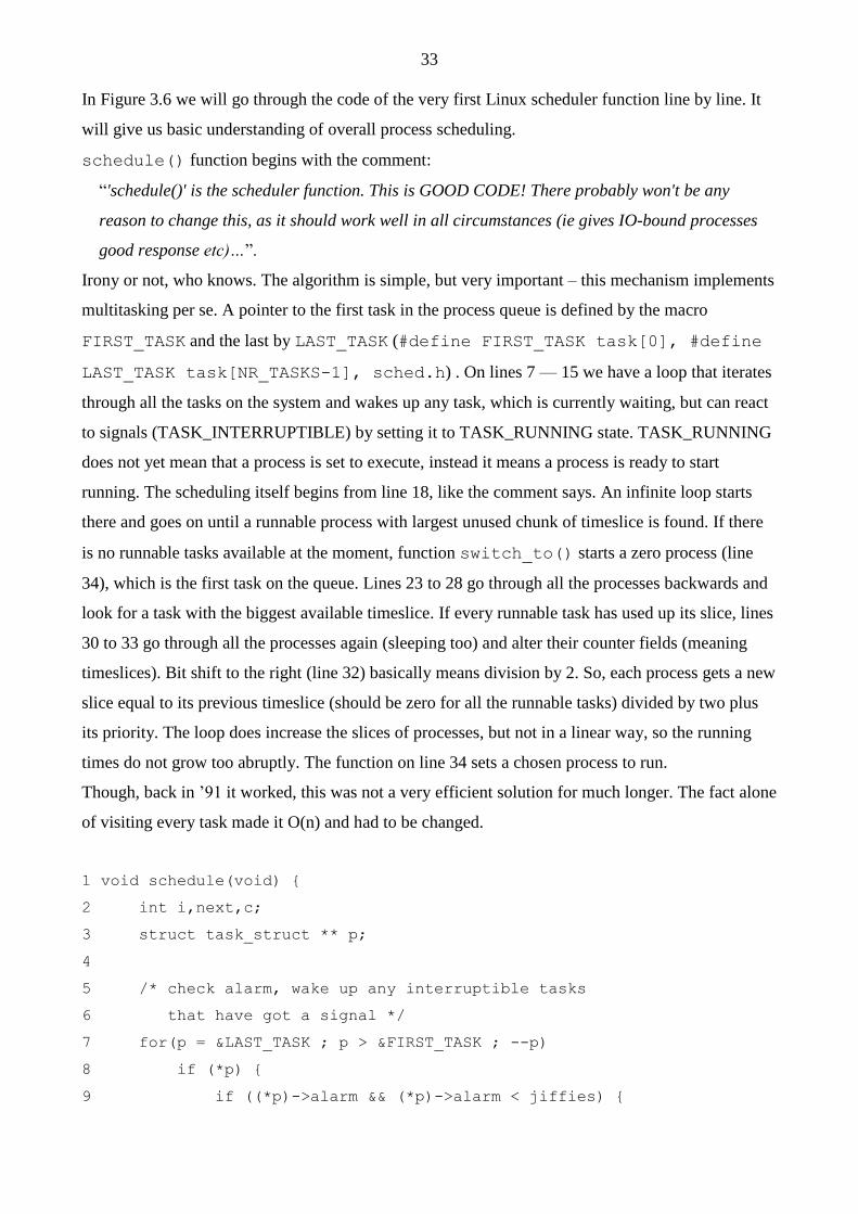
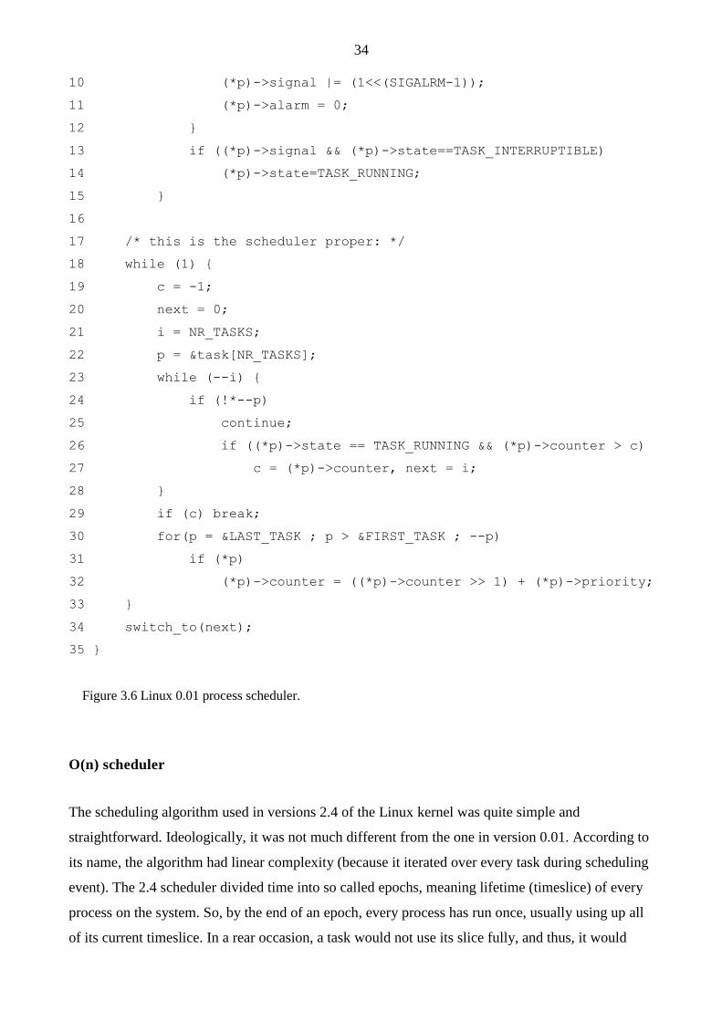
In Figure 3.6 we will go through the code of the very first Linux scheduler function line by line. It
will give us basic understanding of overall process scheduling.
schedule() function begins with the comment:
“'schedule()' is the scheduler function. This is GOOD CODE! There probably won't be any
reason to change this, as it should work well in all circumstances (ie gives IO-bound processes
good response etc)…”.
Irony or not, who knows. The algorithm is simple, but very important – this mechanism implements
multitasking per se. A pointer to the first task in the process queue is defined by the macro
FIRST_TASK and the last by LAST_TASK (#define FIRST_TASK task[0], #define
LAST_TASK task[NR_TASKS-1], sched.h) . On lines 7 — 15 we have a loop that iterates
through all the tasks on the system and wakes up any task, which is currently waiting, but can react
to signals (TASK_INTERRUPTIBLE) by setting it to TASK_RUNNING state. TASK_RUNNING
does not yet mean that a process is set to execute, instead it means a process is ready to start
running. The scheduling itself begins from line 18, like the comment says. An infinite loop starts
there and goes on until a runnable process with largest unused chunk of timeslice is found. If there
is no runnable tasks available at the moment, function switch_to() starts a zero process (line
34), which is the first task on the queue. Lines 23 to 28 go through all the processes backwards and
look for a task with the biggest available timeslice. If every runnable task has used up its slice, lines
30 to 33 go through all the processes again (sleeping too) and alter their counter fields (meaning
timeslices). Bit shift to the right (line 32) basically means division by 2. So, each process gets a new
slice equal to its previous timeslice (should be zero for all the runnable tasks) divided by two plus
its priority. The loop does increase the slices of processes, but not in a linear way, so the running
times do not grow too abruptly. The function on line 34 sets a chosen process to run.
Though, back in ’91 it worked, this was not a very efficient solution for much longer. The fact alone
of visiting every task made it O(n) and had to be changed.
1 void schedule(void) {
2 int i,next,c;
3 struct task_struct ** p;
4
5 /* check alarm, wake up any interruptible tasks
6 that have got a signal */
7 for(p = &LAST_TASK ; p > &FIRST_TASK ; --p)
8 if (*p) {
9 if ((*p)->alarm && (*p)->alarm < jiffies) {
34
10 (*p)->signal |= (1<<(SIGALRM-1));
11 (*p)->alarm = 0;
12 }
13 if ((*p)->signal && (*p)->state==TASK_INTERRUPTIBLE)
14 (*p)->state=TASK_RUNNING;
15 }
16
17 /* this is the scheduler proper: */
18 while (1) {
19 c = -1;
20 next = 0;
21 i = NR_TASKS;
22 p = &task[NR_TASKS];
23 while (--i) {
24 if (!*--p)
25 continue;
26 if ((*p)->state == TASK_RUNNING && (*p)->counter > c)
27 c = (*p)->counter, next = i;
28 }
29 if (c) break;
30 for(p = &LAST_TASK ; p > &FIRST_TASK ; --p)
31 if (*p)
32 (*p)->counter = ((*p)->counter >> 1) + (*p)->priority;
33 }
34 switch_to(next);
35 }
Figure 3.6 Linux 0.01 process scheduler.
O(n) scheduler
The scheduling algorithm used in versions 2.4 of the Linux kernel was quite simple and
straightforward. Ideologically, it was not much different from the one in version 0.01. According to
its name, the algorithm had linear complexity (because it iterated over every task during scheduling
event). The 2.4 scheduler divided time into so called epochs, meaning lifetime (timeslice) of every
process on the system. So, by the end of an epoch, every process has run once, usually using up all
of its current timeslice. In a rear occasion, a task would not use its slice fully, and thus, it would
35
have half of the remaining timeslice added to the new timeslice, allowing it to execute longer during
the next epoch. A lot like in the first scheduler.
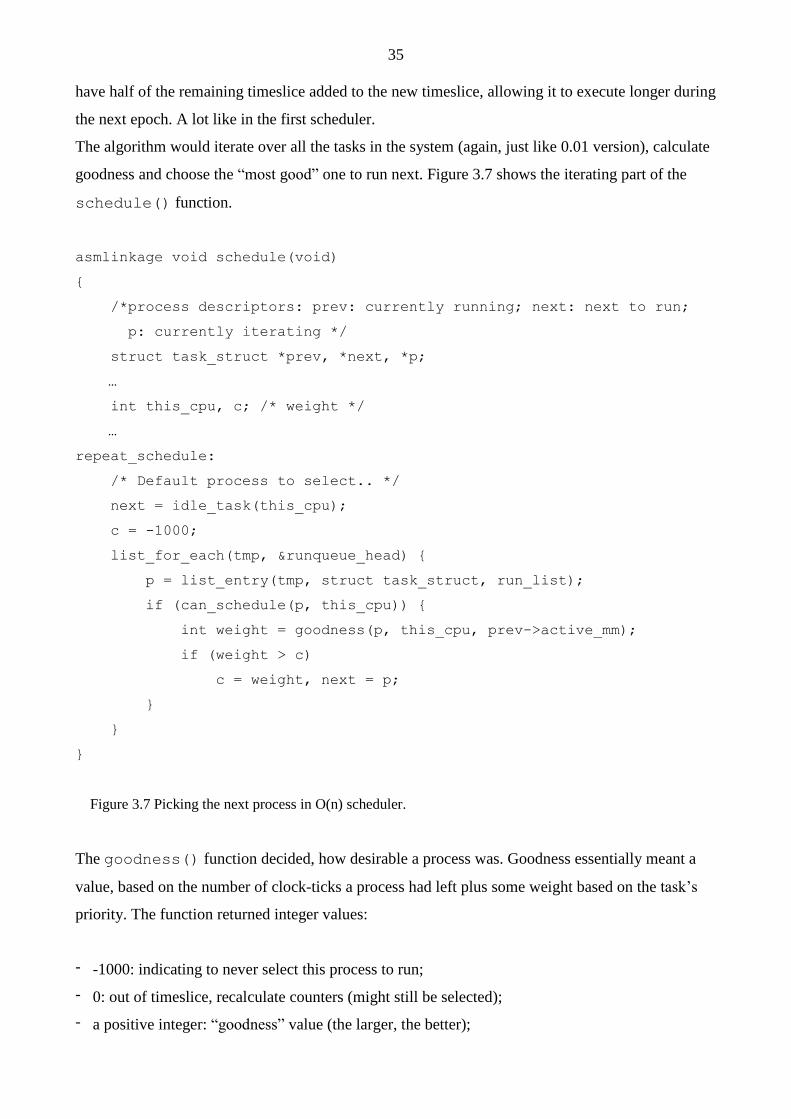
The algorithm would iterate over all the tasks in the system (again, just like 0.01 version), calculate
goodness and choose the “most good” one to run next. Figure 3.7 shows the iterating part of the
schedule() function.
asmlinkage void schedule(void)
{
/*process descriptors: prev: currently running; next: next to run;
p: currently iterating */
struct task_struct *prev, *next, *p;
…
int this_cpu, c; /* weight */
…
repeat_schedule:
/* Default process to select.. */
next = idle_task(this_cpu);
c = -1000;
list_for_each(tmp, &runqueue_head) {
p = list_entry(tmp, struct task_struct, run_list);
if (can_schedule(p, this_cpu)) {
int weight = goodness(p, this_cpu, prev->active_mm);
if (weight > c)
c = weight, next = p;
}
}
}
Figure 3.7 Picking the next process in O(n) scheduler.
The goodness() function decided, how desirable a process was. Goodness essentially meant a
value, based on the number of clock-ticks a process had left plus some weight based on the task’s
priority. The function returned integer values:
- -1000: indicating to never select this process to run;
- 0: out of timeslice, recalculate counters (might still be selected);
- a positive integer: “goodness” value (the larger, the better);
36
- +1000: a real-time process, select this.
Although this approach was relatively simple, it was quite inefficient (spending too much time
choosing the best task on high-end system with thousands of processes) with almost nonexistent
scalability potential, and was weak for real-time systems. It also lacked features to exploit new
hardware architectures such as multicore CPUs.
O(1) scheduler
In early versions of 2.6 kernel, Ingo Molnár introduced a new process scheduler [14] that could
schedule tasks within a constant amount of time (Linux 2.6.8 scheduler did not contain any
algorithms that run in worse than O(1) time) regardless of how many processes were running on the
system. This new code was named the O(1) scheduler; it quickly replaced the old O(n) one on
desktop and server machines.
O(1) scheduler introduced a couple of new features:
- global priority scale, from 0 to 139 with numerically lower values indicating higher priority;
- division between real-time (0 to 99) and normal (100 to 139) processes. Higher priority tasks got
larger timeslices – important processes would run longer;
- early preemption. When a process entered TASK_RUNNING state, the kernel checked, whether
its priority was higher than the one of currently running task’s, and if it was, the scheduler was
invoked to grant CPU to the newly runnable task;
- static priority for real-time tasks;
- dynamic priority for normal tasks, depending on their interactivity. A task’s priority was
recalculated when it finished its timeslice. According to its behavior in the past, level of
interactivity was determined. Interactive tasks were preferred by the scheduler.
Previous versions of process schedulers had an explicit way of recalculating each task’s priority at
the end of an epoch, when all the tasks had used up their timeslices. The processes were kept in one
runqueue (linked list or array). A loop over all the existing processes on the system was run through
every time a switch was in place.
The O(1) method, instead, recalculated a task’s priority at the end of its quanta and maintained two
priority arrays for each available CPU – active and expired. The active array contained all the tasks
in the associated runqueue that had timeslice left. The expired array, in turn, contained all the tasks
37
that had exhausted their timeslice. So, every time a task reached zero, it was transmitted from active
to expired, and priority recalculation of the task was made. This approach allowed to get rid of
recalculation loops and, naturally, minimized the amount of processes being scheduled, as the
scheduler was not taking expired array into account. When all the tasks got their quantum to the
end, the two arrays were just switched. Because the arrays were accessed only with pointers,
switching them did not require looping, simply a pointer swap.
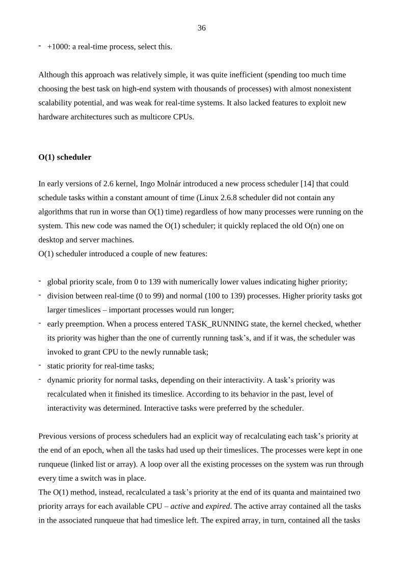
The trick of speeding up the scheduler was in splitting the runqueue into many lists of runnable
processes, one list per priority – as many as 140 lists (Figure 3.8). A runqueue in this case did not
mean an array any more, but a struct instead:
struct runqueue {
unsigned long nr_running; /* number of runnable tasks */
…
struct prio_array *active; /* pointer to the active priority array */
struct prio_array *expired; /* pointer to the expired priority array */
struct prio_array arrays[2]; /* the actual priority arrays */
}
active array expired array
priority task list priority task list
[0] O—-O [0] O—-O—-O
[1] O—-O—-O [1] O
… … …
[139] O [139] O—-O
Figure 3.8 Lists of tasks indexed according to priorities.
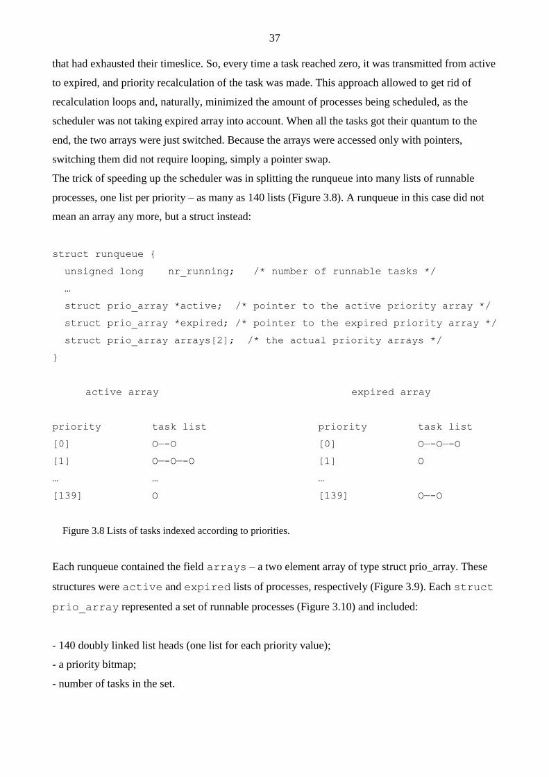
Each runqueue contained the field arrays – a two element array of type struct prio_array. These
structures were active and expired lists of processes, respectively (Figure 3.9). Each struct
prio_array represented a set of runnable processes (Figure 3.10) and included:
- 140 doubly linked list heads (one list for each priority value);
- a priority bitmap;
- number of tasks in the set.
38
________________
_____| active |
| ————————————————
| _ | expired |
| | ———————————————— ___(P0)—(P0)—(P0)
| | | | /
| | | arrays[0] | —————(P1)—(P1)—(P1)
| |->| |
| ————————————————
| | |——————(P0)—(P0)
|———> | arrays[1] |——————(P1)
| |
————————————————
Figure 3.9 The runqueue structure and the two sets of runnable processes.
struct prio_array {
int nr_active; /* number of tasks */
unsigned long bitmap[BITMAP_SIZE]; /* priority bitmap */
struct list_head queue[MAX_PRIO]; /* priority queues */
};
Figure 3.10 Inside priority array.
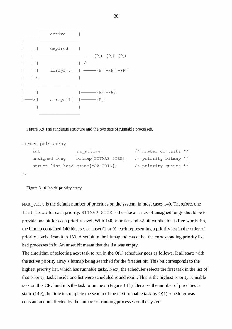
MAX_PRIO is the default number of priorities on the system, in most cases 140. Therefore, one
list_head for each priority. BITMAP_SIZE is the size an array of unsigned longs should be to
provide one bit for each priority level. With 140 priorities and 32-bit words, this is five words. So,
the bitmap contained 140 bits, set or unset (1 or 0), each representing a priority list in the order of
priority levels, from 0 to 139. A set bit in the bitmap indicated that the corresponding priority list
had processes in it. An unset bit meant that the list was empty.
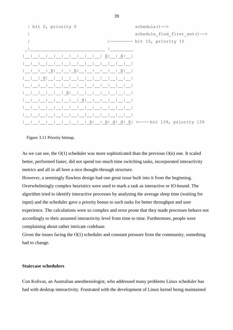
The algorithm of selecting next task to run in the O(1) scheduler goes as follows. It all starts with
the active priority array’s bitmap being searched for the first set bit. This bit corresponds to the
highest priority list, which has runnable tasks. Next, the scheduler selects the first task in the list of
that priority; tasks inside one list were scheduled round robin. This is the highest priority runnable
task on this CPU and it is the task to run next (Figure 3.11). Because the number of priorities is
static (140), the time to complete the search of the next runnable task by O(1) scheduler was
constant and unaffected by the number of running processes on the system.
39
| bit 0, priority 0 schedule()—->
| schedule_find_first_set()—->
| |————————— bit 10, priority 10
_|_____________________________ |_________
|__|__|__|__|__|__|__|__|__|__| X|__|_X|__|
|__|__|__|__|__|__|__|__|__|__|__|__|__|__|
|__|__|__|_X|__|__|_X|__|__|__|__|__|_X|__|
|__|__|_X|__|__|__|__|__|__|__|__|__|__|__|
|__|__|__|__|__|__|__|__|__|__|__|__|__|__|
|__|__|__|__|__|_X|__|__|__|__|__|__|__|__|
|__|__|__|__|__|__|__|_X|__|__|__|__|__|__|
|__|__|__|__|__|__|__|__|__|__|__|__|__|__|
|__|__|__|__|__|__|__|__|__|__|__|__|__|__|
|__|__|__|__|__|__|__|__|_X|__|_X|_X|_X|_X| <———— bit 139, priority 139
Figure 3.11 Priority bitmap.
As we can see, the O(1) scheduler was more sophisticated than the previous O(n) one. It scaled
better, performed faster, did not spend too much time switching tasks, incorporated interactivity
metrics and all in all bore a nice thought-through structure.
However, a seemingly flawless design had one great issue built into it from the beginning.
Overwhelmingly complex heuristics were used to mark a task as interactive or IO-bound. The
algorithm tried to identify interactive processes by analysing the average sleep time (waiting for
input) and the scheduler gave a priority bonus to such tasks for better throughput and user
experience. The calculations were so complex and error prone that they made processes behave not
accordingly to their assumed interactivity level from time to time. Furthermore, people were
complaining about rather intricate codebase.
Given the issues facing the O(1) scheduler and constant pressure from the community, something
had to change.
Staircase schedulers
Con Kolivas, an Australian anesthesiologist, who addressed many problems Linux scheduler has
had with desktop interactivity. Frustrated with the development of Linux kernel being maintained

40
by giant corporations, whose interests lay in server side and database segment, he introduced
several own solutions for more interactive desktop machines.
In 2004 Kolivas released “The Staircase Scheduler” [3]. This patch was aimed at simplifying the
existing obscure code and improving interactive response. It got rid of around 500 lines of old code,
while adding less than 200. Much of what was thrown out was the magic, calculating interactivity
levels; it was replaced with a simple rank-based scheme.
The staircase scheduler implemented runqueue as a ranked array of processes (for each CPU).
Initially, every process was put into the array at the rank of its priority. The scheduler then picked
the first process from the highest available priority. So far, not much had changed.
In the previous algorithm, processes, which had used up their timeslices, were moved to “expired”
array. Staircase did not use this kind of technique. Instead, the expired process would “fall one
priority stair down” – put back into the queue, but at one level lower priority array. The processes,
thus, could continue to run, but with smaller priorities. After exhausting again, a task would go one
step down once more, and so on straight to the bottom.
When a task reached the lowest priority and used up its timeslice it moved back up to one priority
level below its previous maximum and got twice as big a quantum as before. After a task dropped to
the bottom the next time, it got up to two priority levels below maximum and got a timeslice three
times bigger than the original one.
Thus, a process of priority n would fall off the staircase and find itself amongst processes with
priority n-1, but with a bigger timeslice, relative to those other processes. If a process slept for a
long time, it got pushed back to the top of the staircase. Therefore, interactive tasks would usually
stay at the top and be responsive, while batch processes spent much time with the lower priorities,
but executing longer.
In 2007 Con Kolivas made an improvement to his algorithm and released a new scheduler, named
“The Rotating Staircase Deadline Scheduler” or RSDS. Again, aimed at better interactivity, the new
scheduler claimed to be completely starvation free. It brought back the “expired” array and the
concept of an epoch. More on the design of RSDS can be found in the official release
announcement [4]. Later, the scheduler was renamed to “Staircase Deadline” or SD.
Kolivas’ work got a hostile reception in the kernel hacker community for the reasons of it being too
desktop oriented, what Linux at the time was not, and too immature for all possible workload cases
[18]. None of Kolivas’ schedulers were accepted into the mainline and, thus, remained an “out of
tree” work.
Ingo Molnar, the creator of O(1) scheduler and, at the time, the head maintainer of the kernel’s
scheduling policies, then developed the CFS (Completely Fair Scheduler) based on some of the
ideas of fairness incorporated within the staircase design.
41
3.4 CFS
The Completely Fair Scheduler (CFS) was merged into the Linux kernel version 2.6.23 in early
2007 [14] and has been the default scheduler since then.
As the documentation to the kernel states, 80% of CFS design can be summed up in a single
sentence: CFS basically models an “ideal, precise multitasking CPU” on real hardware.
Let us dig into the meaning of an ideal, perfectly multitasking processor. In such a system, with n
running processes, each process would be having 1/n amount of CPU-time while running constantly
– in any measurable period all the tasks would have run for the same amount of wall-clock time.
For example, given 10 milliseconds, if there were two batch tasks executing, a normal scheduler
would offer them 5 milliseconds with 100% CPU power each. An ideal processor would run them
both simultaneously for 10 milliseconds with each getting 50% CPU. The later model is called
perfect multitasking.
This is of course impractical – it is physically impossible to run any more than one execution flow
on a single processor(core). So, CFS tries to mimic perfectly fair scheduling. Rather than simply
assign a timeslice to a process, the scheduler calculates how long a task should run as a function of
the total number of currently runnable processes. As it was mentioned earlier, instead of just setting
a nice value to a task, the scheduler uses it to weight a proportion of the CPU the process is to
receive. Higher priority jobs get larger weights, meaning more CPU-time.
CFS achieves fairness by letting a task run for a period, proportional to its weight divided by the
total weight of all runnable processes. To calculate the actual timeslice, CFS sets a bounded target
(amount of time) for the approximation [15]. With the target of 10 milliseconds, if we had two tasks
of the same priority, each task would run for 5 milliseconds, if we had five tasks, each would run
for 2 milliseconds and if we had ten runnable tasks, they would be given 1 millisecond each. This
applies regardless of the priority level the tasks are at, as long as it is the same, and there are no
other runnable tasks at different priorities.
As the number of tasks approaches infinity, timeslices of processes approach zero. Luckily, CFS
has a ground limit for a quantum, so that content switching would not overtake all the processor
time. Usually it is 1 millisecond. In a situation, where a target time is not enough to schedule all the
tasks, it is simply enlarged (the default target is around 20 milliseconds and added chunks are
usually around 4 milliseconds).
When priorities differ, CFS will still stay fair and square. Take a target of 20 milliseconds and two
processes, one with niceness of 0 (the default), the other with niceness of 5. The proportional
difference between the corresponding weights will be calculated as roughly 1/3, meaning that the
higher priority process receives a timeslice of approximately 15 milliseconds while the lower
42
priority process receives a timeslice of 5 milliseconds. Now consider two processes with the
niceness values of 5 and 10 respectively. While the absolute niceness is larger in this case, the
relative difference between the niceness values is the same as in the previous example, yielding an
identical timeslice division.
In general, CFS is called fair, because it gives each process the share of the CPU, relative to other
tasks.
Runqueue
The design of completely fair scheduler is quite radical – it does not use the old data structures for
the runqueues, but it uses a time-ordered red-black tree, often called rbtree, (defined in
<include/linux/rbtree.h>) to build a "timeline" of future task execution, and thus has
neither separate arrays for running and expired tasks no array switches that the previous O(1)
scheduler and RSDL/SD had. The key values of the tree nodes are virtual run times of processes (a
function of how long a process should run). The smaller the key, the more to the left of the tree a
node is. The scheduler always picks the leftmost node as the next task to run. We will discuss
virtual run times later in this chapter in greater details.
The rbtree data structure is represented by struct cfs_rq, which is embedded into each per-
CPU runqueue structure of the base Linux scheduler (struct rq), we discussed earlier. In
<kernel/sched/sched.h>:
struct cfs_rq {
struct load_weight load;
unsigned int nr_running, …;
u64 min_vruntime;
struct rb_root tasks_timeline;
struct rb_node *rb_leftmost;
/*
* 'curr' points to currently running entity on this cfs_rq.
* It is set to NULL otherwise (i.e when none are currently running).
*/
struct sched_entity *curr, …;
…
}
43
The fields are as follows:
- nr_running holds the amount of runnable tasks on this queue and
- load contains the cumulative weight of them all;
- min_vruntime: the smallest vruntime on the runqueue. This variable maintains the time for
a task which has run for the least amount of time on the CPU. Note, that this is a single variable
for the entire runqueue, so it serves as a singular benchmark for all the tasks to be compared
against. The task, which has run the least, can be found out by subtracting min_vruntime
from the task’s vruntime. If the resulting number is big, the task clearly has run for long – the
smaller the result, the sooner the task will get the CPU again;
- tasks_timeline: the root the rbtree, representing runnable tasks in CFS runqueue;
- rb_leftmost: the element that will be scheduled next. In an rbtree it is the leftmost element,
because the tree is sorted based on vruntime of processes (smaller vruntime means sooner
execution);
- curr points to the scheduling entity of the currently running process.
Scheduling entities
As mentioned above, the default Linux scheduler (CFS) can work with more general entities than
tasks. The structure to describe a scheduling entity is defined in <include/linux/sched.h>
header file and mostly contains attributes for accounting run time of processes (or other
encapsulated essences):
struct sched_entity {
struct load_weight load; /* for load-balancing */
struct rb_node run_node;
…
unsigned int on_rq;
u64 exec_start;
u64 sum_exec_runtime;
u64 vruntime;
u64 prev_sum_exec_runtime;
};
44
The fields are as follows:
- load: the calculated load weight of each particle combined into one entity;
- run_node: a red-black tree node;
- on_rq: is the entity currently in a runqueue on not.
- exec_start: when a process starts running on a CPU, the timestamp is taken and stored in
this variable;
- sum_exec_runtime is used for storing the time a process has been running in total (for the
completely fair scheduler to make decisions). Tracking is done by calling the function
update_curr() from numerous places in the kernel code. At every invocation, the difference
between current time and the timestamp in exec_start is added to sum_exec_runtime
and exec_start is updated to current time.
- vruntime: for how long this entity has run on a CPU, based on a virtual clock;
- prev_sum_exec_runtime: used for storing the previous run time of a process. When it is
taken off the CPU, sum_exec_runtime is copied into this variable. The information will be
later used by the scheduler. Note, that sum_exec_runtime is not reset.
The scheduler entity is embedded in process descriptor structure as a member variable named se.
Keep in mind that a single task is always a scheduler entity, but a scheduler entity can be more than
a single task.
Virtual clock
Throughout this chapter a mysterious vruntime counter has occurred in the code. Now it is time to
reveal the secret behind this phantom notion. Mimicking the perfect fairness, CFS uses virtual clock
to measure the amount of time a waiting process would have been allowed to run on a completely
fair processor [15]; each scheduling entity is packed with vruntime variable to store this value.
There is no actual implementation of virtual clock, however. The concept is a pure abstraction. All
the information needed to calculate virtual run time, can be acquired using actual time and a task’s
load weight. The calculations are implemented inside update_curr() function, which updates
time accounting fields of scheduling entities and min_vruntime of a CFS runqueue. In
<kernel/sched/fair.c>:
45
/*
* Update the current task's runtime statistics.
*/
static void update_curr(struct cfs_rq *cfs_rq)
{
struct sched_entity *curr = cfs_rq->curr;
u64 now = rq_clock_task(rq_of(cfs_rq));
u64 delta_exec;
if (unlikely(!curr))
return;
delta_exec = now - curr->exec_start;
…
curr->vruntime += calc_delta_fair(delta_exec, curr);
update_min_vruntime(cfs_rq);
…
}
The function first gets the currently executing process of the runqueue and the actual clock value of
the main scheduler queue (struct rq) on this CPU. If no process is currently running (unlikely,
though), there is nothing to do. Otherwise, time is computed between task’s starting and now, and
stored in delta_exec variable. Some uninteresting statistics are updated after that (not shown
here). Next, the function delegates the work of calculating vruntime to calc_delta_fair():
static inline u64 calc_delta_fair(u64 delta, struct sched_entity *se)
{
if (unlikely(se->load.weight != NICE_0_LOAD))
delta = __calc_delta(delta, NICE_0_LOAD, &se->load);
return delta;
}
If the process has the default priority (internal niceness of 120), its virtual runtime is the same as
actual running time. If the task does not have default priority, vruntime is calculated inside
__calc_delta(), which can be found in the same source file. The function contains some black
magic of bit shifting and inverting, but in general it all boils down to the formula
46
delta = delta_exec * NICE_0_LOAD / curr->load.weight;
At last, the update_curr() function calls update_min_vruntime() to update
min_vruntime of the runqueue. The kernel checks, if there exists a leftmost node in the tree, that
is, the next task to be run (it has the smallest vruntime). The kernel takes vruntime of the
leftmost element in the tree, if it exists, or that of a currently running process, depending on which
is smaller. If no leftmost element can be found – the tree is empty – the virtual run time of the
current process is used. Then the kernel calculates the maximum of current min_vruntime and
the minimum value of vruntime from before, to insure that min_vruntime increases
monotonically and never decreases:
static void update_min_vruntime(struct cfs_rq *cfs_rq)
{
u64 vruntime = cfs_rq->min_vruntime;
if (cfs_rq->curr)
vruntime = cfs_rq->curr->vruntime;
if (cfs_rq->rb_leftmost) {
struct sched_entity *se = rb_entry(cfs_rq->rb_leftmost,
struct sched_entity,
run_node);
if (!cfs_rq->curr)
vruntime = se->vruntime;
else
vruntime = min_vruntime(vruntime, se->vruntime);
}
/* ensure we never gain time by being placed backwards. */
cfs_rq->min_vruntime = max_vruntime(cfs_rq->min_vruntime, vruntime);
…
}
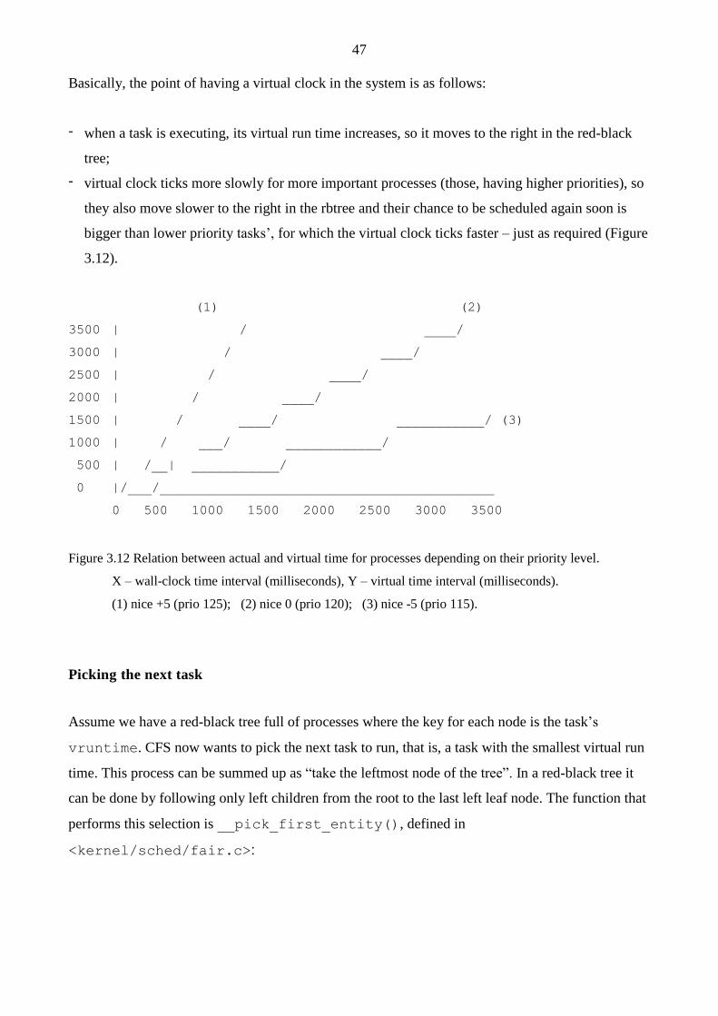
47
Basically, the point of having a virtual clock in the system is as follows:
- when a task is executing, its virtual run time increases, so it moves to the right in the red-black
tree;
- virtual clock ticks more slowly for more important processes (those, having higher priorities), so
they also move slower to the right in the rbtree and their chance to be scheduled again soon is
bigger than lower priority tasks’, for which the virtual clock ticks faster – just as required (Figure
3.12).
(1) (2)
3500 | / ____/
3000 | / ____/
2500 | / ____/
2000 | / ____/
1500 | / ____/ ___________/ (3)
1000 | / ___/ ____________/
500 | /__| ___________/
0 |/___/__________________________________________
0 500 1000 1500 2000 2500 3000 3500
Figure 3.12 Relation between actual and virtual time for processes depending on their priority level.
X – wall-clock time interval (milliseconds), Y – virtual time interval (milliseconds).
(1) nice +5 (prio 125); (2) nice 0 (prio 120); (3) nice -5 (prio 115).
Picking the next task
Assume we have a red-black tree full of processes where the key for each node is the task’s
vruntime. CFS now wants to pick the next task to run, that is, a task with the smallest virtual run
time. This process can be summed up as “take the leftmost node of the tree”. In a red-black tree it
can be done by following only left children from the root to the last left leaf node. The function that
performs this selection is __pick_first_entity(), defined in
<kernel/sched/fair.c>:
48
struct sched_entity *__pick_first_entity(struct cfs_rq *cfs_rq)
{
struct rb_node *left = cfs_rq->rb_leftmost;
if (!left)
return NULL;
return rb_entry(left, struct sched_entity, run_node);
}
Note, that the code does not go through the tree to find the leftmost node. Recall, that cfs_rq
structure keeps a pointer to it (the pointer is assigned when adding tasks to the tree)? While finding
the next process to run would not be an expensive operation – O(log n) for n nodes in the tree – it is
even easier to cache the leftmost node. If the return value from this function is NULL, there are no
processes in the tree, and CFS schedules the idle task.
3.5 Real-time scheduler
From the very first versions of Linux, the scheduler was real-time POSIX compatible. With
development of the scheduling classes, rt processes became manageable by a separate scheduler,
defined in <kernel/sched/rt.c>. CFS only needs to be aware of existence of such different
processes on the system, but it has no affiliation to them whatsoever.
The essence
In the eyes of the system, real-time processes have one significant difference compared to all the
others – if there is a runnable rt task, it will be put to run. Unless there is an rt task with a higher
priority. Two types of policies exist for real-time processes:
- SCHED_FIFO: basic first in first out scheduling algorithm. Tasks obeying this policy do not
have timeslices, they run until they block or yield the CPU voluntarily or get preempted by a
higher priority real-time task. A SCHED_FIFO task preempts any SCHED_NORMAL process.
Several SCHED_FIFO tasks of the same priority run round robin – when a task is done, it is put
to the end of the queue and the next task starts;
49
- SCHED_RR: identical to SCHED_FIFO, but with timeslices. Tasks of the same priority run
round robin until preempted by a more important task or until they use their quantum to the end.
When a timeslice is up, it is refilled, and a task is put to the end of the queue. The default
timeslice for SCHED_RR tasks is defined in <include/linux/sched/rt.h> and, on
desktop machines, is equal to 100 milliseconds:
#define RR_TIMESLICE (100 * HZ / 1000)
The kernel gives real-time tasks a static priority, which does not get dynamically recalculated; the
only way to change niceness is by hand with the chrt command. This ensures that an rt task
always preempts a normal one and that strict order is kept between rt tasks of different priorities.
Representation
Real-time processes have their own schedulable entity structure, defined in
<include/linux/sched.h>:
struct sched_rt_entity {
struct list_head run_list;
unsigned long timeout;
unsigned long watchdog_stamp;
unsigned int time_slice;
…
struct sched_rt_entity *back;
…
struct sched_rt_entity *parent;
/* rq on which this entity is (to be) queued: */
struct rt_rq *rt_rq;
…
};
Timeslice for SCHED_FIFO is zero, because none is needed (<kernel/sched/rt.c>):
int sched_rr_timeslice = RR_TIMESLICE;
…
50
static unsigned int get_rr_interval_rt(struct rq *rq,
struct task_struct *task)
{
/*
* Time slice is 0 for SCHED_FIFO tasks
*/
if (task->policy == SCHED_RR)
return sched_rr_timeslice;
else
return 0;
}
The main runqueues also contain sub-runqueues for real-time tasks,
<kernel/sched/sched.h>:
/* Real-Time classes' related field in a runqueue: */
struct rt_rq {
struct rt_prio_array active;
unsigned int rt_nr_running;
…
struct rq *rq; /* main runqueue */
};
/*
* This is the priority-queue data structure of the RT scheduling class:
*/
struct rt_prio_array {
/* include 1 bit for delimiter */
DECLARE_BITMAP(bitmap, MAX_RT_PRIO+1);
struct list_head queue[MAX_RT_PRIO];
};
All real-time tasks of the same priority are kept in a linked list in active.queue[prio] and,
like in the O(1) scheduler, there is a bitmap (active.bitmap), signalizing that a particular queue
is not empty.
Very much like update_curr() in CFS, there is a update_curr_rt() function in real-time
scheduler. It keeps track of the time rt tasks spend on the CPU, gathers some statistics, updates
51
timeslices where needed and calls the scheduler when appropriate. All calculations are done using
actual time, no virtual clock is used.
When dealing with real-time on Linux, remember that despite current kernel versions can meet
pretty stringent timing requirements, there is only soft real-time and no guarantees are given.
3.6 BFS
In August 2009, a veteran Linux enthusiast Con Kolivas released the first version of the new
process scheduler for the kernel under a provocative title “Brain Fuck Scheduler” or BFS [10]. New
Kolivas’ work is still aimed at enhancing desktop interactivity and responsiveness; it scales best on
portable devices and machines with less than 16 CPUs (in contrast, CFS is mainly designed for
servers and huge clusters with thousands of processor cores). This time Kolivas intentionally left his
code out of the main Linux source tree and distributes it as a separate entity, widely known as “–ck
patch set”. A new version is released every time the kernel updates and latest revision dates on
31.12.2014, indicating that active development is going on to this day.
The goal of BFS is to provide a CPU process scheduler with simplistic design and small, easily
maintainable code base instead of huge complex monstrosities of previous schedulers with their
heuristics and tuning knobs that are difficult to understand, impossible to model and to predict the
effect of, and when tuned to one workload, are causing massive regressions to another. When first
released, for the kernel 2.6.31, BFS codebase was approximately 9000 lines of code smaller than
the existing mainline Linux scheduler at the time.
The design of BFS brings back a single queue of runnable processes, regardless of the number of
CPUs available. The reason for introducing a one queue structure is in maintaining simplicity. Once
multiple runqueues are used, per-CPU or otherwise, there is always complex interactions between
them in the sake of consistency – as each runqueue is responsible only for its own processes and
maintains fairness only locally. Any advantage in throughput of having CPU local tasks causes
other disadvantages. The system ought to have a complex balancing mechanism to keep fairness
between CPUs and can maintain relatively low latency only for tasks, bound to the same processor,
as “jumps” across CPUs are indeed expensive.
Current Linux scheduler tends to determine whether a task is interactive or processor bound by
analysing its sleep/run time durations. Kolivas asserts that these kinds of interactivity estimators are
doomed to fail, because it is close to impossible to detect if a task is sleeping voluntarily, as in user
space application waiting for a key press, or because it is waiting for a signal from another thread,

52
input/output operation or whatever else. In BFS, all accounting is done purely based on tasks
utilizing CPU; nowhere sleep time is used in any way to estimate interactivity.
Runqueue
As mentioned previously, BFS has only one runqueue for all the CPUs on the system and it is
global (Figure 3.13). The global runqueue in BFS has 103 priority queues, each of which is a
doubly linked list. First 100 are dedicated to real-time tasks, 101st is for SCHED_ISO (isochronous,
will be discussed later on the chapter in greater detail), 102nd for SCHED_NORMAL and 103rd for
SCHED_IDLEPRIO (idle priority scheduling). The order of priorities grows from 0 to 103, zero
being the most important and 103 the most unwanted. BFS, much like the O(1) scheduler, uses a
bitmap to look up priority queues that have runnable tasks inside. When a new task enters runnable
state, the bit of the corresponding priority is set.
#define MAX_USER_RT_PRIO 100
#define MAX_RT_PRIO (MAX_USER_RT_PRIO + 1)
#define ISO_PRIO (MAX_RT_PRIO)
#define NORMAL_PRIO (MAX_RT_PRIO + 1)
#define IDLE_PRIO (MAX_RT_PRIO + 2)
#define PRIO_LIMIT ((IDLE_PRIO) + 1)
/* There can be only one */
static struct global_rq grq;
/*
* The global runqueue data that all CPUs work off. Data is protected
* either by the global grq lock, or the discrete lock that precedes the
* data in this struct.
*/
struct global_rq {
raw_spinlock_t lock;
unsigned long nr_running;
unsigned long nr_uninterruptible;
…
struct list_head queue[PRIO_LIMIT];
DECLARE_BITMAP(prio_bitmap, PRIO_LIMIT + 1);
53
u64 niffies; /* Nanosecond jiffies */
}
Figure 3.13 Global priority queue in BFS.
Rather interesting field here is niffies, which is basically the same as jiffies, but in
nanoseconds. For those, who skipped their lessons on operating systems: the global variable
jiffies holds the number of timer interrupts since the Linux system booted up. There are HZ
jiffies in a second. An average desktop system would normally have HZ set to 1000. So, on a
desktop, niffies would hold seconds from boot up * 1 000 000 000.
Virtual deadline
There is only one priority sub-queue for each type of scheduling policy, except real-time (and rt
tasks run round robin). So, the scheduler has to know which task to pick next from a list of same
priority processes. For achieving fairness and for nice level distribution BFS uses mechanism called
virtual deadline.
When a task enters runnable state, it gets a timeslice, equal to rr_interval, which is a tunable
value, set to 6 milliseconds by default, and a virtual deadline. A timeslice is always the same for all
the processes of all priorities:
/*
* This is the time all tasks within the same priority round robin.
* Value is in ms and set to a minimum of 6ms.
* Scales with number of cpus. Tuneable via /proc interface.
*/
int rr_interval __read_mostly = 6;
/*
* The quota handed out to tasks of all priority levels when refilling
* their time_slice.
*/
static inline int timeslice(void)
{
return MS_TO_US(rr_interval);
}
54
The __read_mostly macro is meant to inform the compiler that this piece of data will not be
modified very often and will mostly be just read, hence the read mostly. On multiprocessor systems,
each CPU can copy such a value to itself (cache) in order to speed up reading.
Deadline is calculated using the niffies counter inside the global runqueue. It is “now” (in
niffies) + (offset by priority):
grq.niffies + prio_ratios[user_prio] * rr_interval * (MS_TO_NS(1) / 128);
prio_ratios[user_prio] means priority, proportional to user given niceness, it increases by
10% every nice level starting from nice -20.
In an event of rescheduling, the deadline is used to determine, which task will be run next. There is
no guarantee though that a process will be selected after reaching its deadline, that is why it is
called virtual. There are three ways to switch running processes in BFS. The first is when a task
uses its timeslice to the end. The task is taken off the CPU, the timeslice refilled and the deadline
reset using the formula above. The second way is when a process goes to sleep. Timeslice and
deadline are not touched in this situation, they will be carried on when the task wakes up. The third
way is preemption – a newly woken task, having higher priority or an earlier deadline than that of a
currently running task’s, takes the processor over. On the first and second cases, after a task gives
the CPU up, the scheduler loops through all the queued processes to determine which has the
earliest deadline – thus resulting in O(n) lookup behavior – and that task is then chosen to execute.
Task lookup
When the scheduler is called to set a new task to run, the lookup happens in the following way. The
bitmap is checked for set bits starting from highest priority:
static inline struct
task_struct *earliest_deadline_task(struct rq *rq,
int cpu,
struct task_struct *idle)
{
struct task_struct *edt = NULL;
unsigned long idx = -1;
do {
struct list_head *queue;
55
struct task_struct *p;
u64 earliest_deadline;
idx = next_sched_bit(grq.prio_bitmap, ++idx);
if (idx >= PRIO_LIMIT)
return idle;
queue = grq.queue + idx;
If a real-time priority is found, the corresponding queue will be checked and, if CPU affinity allows,
the first task in there will be scheduled to run (rt processes run round-robin):
// same do-loop continues
if (idx < MAX_RT_PRIO) {
/* We found an rt task */
list_for_each_entry(p, queue, run_list) {
/* Make sure cpu affinity is ok */
if (needs_other_cpu(p, cpu))
continue;
edt = p;
goto out_take;
}
/*
* None of the RT tasks at this priority can run on
* this cpu
*/
continue;
}
If there are no runnable real-time tasks, the scheduler checks other priority bits in the bitmap and
their process lists in order. The SCHED_ISO priority is checked first, and all SCHED_ISO tasks
have the same priority value, so they're selected by the earliest deadline value. If no SCHED_ISO
tasks are found, SCHED_NORMAL tasks are selected by the earliest deadline. Finally if no
SCHED_NORMAL tasks are found, SCHED_IDLEPRIO tasks are selected by the earliest deadline.
56
Here the scheduling becomes O(n) – the code goes through the entire list to choose a task (provided
it has suitable affinity):
// same do-loop continues
/*
* No rt tasks. Find the earliest deadline task. Now we’re
* in O(n) territory.
*/
earliest_deadline = ~0ULL;
list_for_each_entry(p, queue, run_list) {
u64 dl;
/* Make sure cpu affinity is ok */
if (needs_other_cpu(p, cpu))
continue;
…
dl = p->deadline;
if (deadline_before(dl, earliest_deadline)) {
earliest_deadline = dl;
edt = p;
}
}
} while (!edt);
out_take:
take_task(cpu, edt);
return edt;
}
The hack ~0ULL is not something you want to use in your code, but it basically means maximum
unsigned 64-bit value. deadline_before(u64 deadline, u64 time) checks if the
“deadline” is smaller than “time”.

57
Isochronous and idleprio scheduling
Isochronous scheduling is a unique policy, brought by BFS, designed to provide users without super
user privileges with performance close to real-time. The policy is defined as SCHED_ISO. Tasks of
this scheduling policy have their priority between SCHED_NORMAL and true real-time processes.
SCHED_ISO tasks run purely round robin, at rr_interval rate, between each other.
BFS includes an internal check, if a task is trying to obtain real-time priority, but lacks the needed
permissions, it will be put to SCHED_ISO policy instead. Once a task has been set to SCHED_ISO
policy, it will need super user privileges to go back to SCHED_NORMAL. This will ensure that the
task remains “almost real-time”, no matter what, and that its child processes will inherit the ISO
policy.
IDLE_PRIO policy is that of the lowest priority on the system. Tasks that otherwise would not get
to run, are set to this scheduling policy and are run only if there are no other jobs to do. This is
ideally suited, for example, for seti@HOME distributed computations or for some batch processes
that shall not cause any slowdown to the foreground tasks. As with the isochronous tasks, once a
process is set to be IDLE_PRIO, it needs super user privileges to go back to SCHED_NORMAL.
58
4. Conclusion
Process scheduling has always been and always will be the corner stone in operating systems’
development. It seems to remain one of those things, eternally unfinished. Best programming gurus
in the world can work on the CPU scheduler for a while, carefully designing every step and making
it perform better, only to notice that it serves only some workloads good, some others fairly well
and the rest of them poorly. Users of desktop systems, in particular, are very demanding about
scheduler latencies. In response, the current Linux scheduler has grown large, adopted the many
heuristics of all kinds and became intricate to the point of obfuscation. But if there is one constant
with open source operating systems like Linux, it is that they never stop changing. Now we have
CFS as the main scheduler. It can satisfy many and make many unhappy with its performance.
Thus, there will be attempts to improve the algorithms further and further to perfection. Thanks to
kernel hackers all over the globe and especially to Ingo Molnar and to Con Kolivas, we have a
decent level of scheduling fairness on our systems today.
59
References
[1] Daniel P. Bovet and Marco Cesati, Understanding the Linux Kernel, Third Edition.
O'Reilly Media, 2005.
[2] Chris Cooper and Chris Moore, HP-UX 11i Internals. Prentice Hall, 2004
[3] Jonathan Corbet, The staircase scheduler. http://lwn.net/Articles/87729 Checked 05.02.2015.
[4] Jonathan Corbet, The Rotating Staircase Deadline Scheduler.
http://lwn.net/Articles/224865 Checked 05.02.2015 Checked 05.02.2015.
[5] Christoph Lameter, SLUB: The unqueued slab allocator V6.
http://www.lwn.net/Articles/229096 Checked 05.02.2015.
[6] Ilkka Haikala ja Hannu‐Matti Jarvinen, Kayttojarjestelmat. Talentum, 2004.
[7] Randall Hyde, The Art of Assembly Language. No Starch Press, 2010.
[8] ISO/IEC, ISO/IEC 9899:1999(E): Programming Languages – C. 1999.
[9] Jane W. S. Liu, Real-Time Systems. Prentice Hall, 2000.
[10] Con Kolivas, FAQS about BFS. http://ck.kolivas.org/patches/bfs/bfs-faq.txt
Checked 05.02.2015.
[11] Christoph Lameter and Linus Torvalds, Make SLUB the default allocator.
http://git.kernel.org/cgit/linux/kernel/git/torvalds/linux.git/commit/?id=a0acd820807680d2c
cc4ef3448387fcdbf152c73 Checked 05.02.2015.
[12] Robert Love, Linux Kernel Development (3rd Edition). Addison-Wesley
Professional, 2010.
[13] Robert Love, Linux System Programming: Talking Directly to the Kernel and C Library
(Second Edition). O'Reilly Media, 2013.
[14] Ingo Molnar, Modular Scheduler Core and Completely Fair Scheduler.
https://lkml.org/lkml/2007/4/13/180 Checked 05.02.2015.
[15] Wolfgang Mauerer, Professional Linux Kernel Architecture. Wrox, 2008.
[16] Richard McDougall and Jim Mauro, Solaris Internals: Solaris 10 and OpenSolaris Kernel
Architecture (2nd Edition). Prentice Hall, 2006.
[17] Tom Shanley, x86 Instruction Set Architecture. MindShare Press, 2010.
[18] Linus Torvalds, Subject: Re: Linus 2.6.23-rc1. E-mail in Linux Kernel Mailing List.
https://lkml.org/lkml/2007/7/27/426 Checked 05.02.2015.
[19] The Institute of Electrical and Electronics Engineers IEEE Standards Project P1003.1c,
Threads Extensions for Portable Operating Systems. Issue 6, 1995.
[20] The Institute of Electrical and Electronics Engineers IEEE Standards Project P1003.1b,
Real-time Extension for Portable Operating Systems. 1993.