Duquesne UniversityDuquesne Scholarship Collection

Electronic Theses and Dissertations

Spring 5-11-2018

A Computational Model of Team-based Dynamicsin the Workplace: Assessing the Impact ofIncentive-based Motivation on ProductivityJosef Di Pietrantonio

Follow this and additional works at: https://dsc.duq.edu/etd

Part of the Industrial and Organizational Psychology Commons, Organization DevelopmentCommons, and the Other Applied Mathematics Commons

This Immediate Access is brought to you for free and open access by Duquesne Scholarship Collection. It has been accepted for inclusion in ElectronicTheses and Dissertations by an authorized administrator of Duquesne Scholarship Collection. For more information, please contactphillipsg@duq.edu.

Recommended CitationDi Pietrantonio, J. (2018). A Computational Model of Team-based Dynamics in the Workplace: Assessing the Impact of Incentive-based Motivation on Productivity (Master's thesis, Duquesne University). Retrieved from https://dsc.duq.edu/etd/1424

A COMPUTATIONAL MODEL

OF TEAM-BASED DYNAMICS IN THE WORKPLACE:

ASSESSING THE IMPACT OF INCENTIVE-BASED MOTIVATION

ON PRODUCTIVITY

A Thesis

Submitted to the McAnulty College and Graduate School of Liberal Arts

Duquesne University

In partial fulfillment of the requirements for

the degree of Masters of Science in Computational Mathematics

By

Josef Di Pietrantonio

May 2018

Copyright by

Josef Di Pietrantonio

2018

A COMPUTATIONAL MODEL

OF TEAM-BASED DYNAMICS IN THE WORKPLACE:

ASSESSING THE IMPACT OF INCENTIVE-BASED MOTIVATION

ON PRODUCTIVITY

By

Josef Di Pietrantonio

Approved April 9, 2018

Dr. Rachael Miller NeilanAssociate Professor of Mathematics(Committee Chair)

Dr. James SwindalDean, McAnulty College and GraduateSchool of Liberal ArtsProfessor of Philosophy

Dr. James B. SchreiberProfessor, School of Nursing(Committee Member)

Dr. John KernChair, Department of Mathematics andComputer ScienceAssociate Professor of Statistics

iii

ABSTRACT

A COMPUTATIONAL MODEL

OF TEAM-BASED DYNAMICS IN THE WORKPLACE:

ASSESSING THE IMPACT OF INCENTIVE-BASED MOTIVATION ON

PRODUCTIVITY

By

Josef Di Pietrantonio

May 2018

Thesis supervised by Rachael Miller Neilan, Ph.D., Associate Professor

Large organizations often divide workers into small teams for the completion of essential

tasks. In an e↵ort to maximize the number of tasks completed over time, it is common

practice for organizations to hire workers with the highest level of education and experience.

However, despite capable workers being hired, the ability of teams to complete tasks may

su↵er if the workers’ individual motivational needs are not satisfied.

To explore the impact of incentive-based motivation on the success of team-based orga-

nizations, we developed an agent-based model that stochastically simulates the proficiency

of 100 workers with varying abilities and motive profiles to complete time-sensitive tasks

in small teams. The model is initialized by randomly assigning each of the 100 workers an

ability value (1 through 5) and a motive profile from initial probability distributions. A

motive profile is a 3-parameter equation that quantifies a worker’s tendency to actualize his

or her potential based on the individual’s motivational needs for a�liation, achievement,

and power. The model creates new tasks as workers become available; each new task is

assigned a random di�culty value and a team of 2 to 4 workers. During each time step,

each worker contributes to their assigned task at a rate determined by the worker’s ability

iv

and motive profile. At the end of 365 time steps (1 year), the model outputs the total

number of completed tasks, which is the primary measurement of productivity. By simu-

lating the model hundreds of times for di↵erent sets of initial distributions and analyzing

output, we are able to determine which worker attributes lead to increased team-based

productivity. Results aid in understanding optimal hiring and human resource allocation

in a team-based organization.

v

AKNOWLEDGEMENTS

I would like to sincerely thank Dr. Rachael Miller Neilan for the exceptional guidance

throughout this thesis experience. Her work ethic and determination was inspiring and

the driver of progress and success. She helped me actualize an idea into a model, paper,

and presentation I am truly proud of. I would also like to thank Dr. James Schreiber for

his consultations on motivation theory, as well as for the encouragement of and excitement

about this interdisciplinary thesis topic.

vi

Contents

1 Introduction 1

2 Incentive-based Motivation 3

2.1 Theory . . . . . . . . . . . . . . . . . . . . . . . . . . . . . . . . . . . . . . 3

2.2 Mathematical model . . . . . . . . . . . . . . . . . . . . . . . . . . . . . . 6

3 Computational Model 9

3.1 What is an agent-based model? . . . . . . . . . . . . . . . . . . . . . . . . 9

3.2 Entities and scales . . . . . . . . . . . . . . . . . . . . . . . . . . . . . . . 10

3.3 Process overview and scheduling . . . . . . . . . . . . . . . . . . . . . . . . 13

3.4 Design concepts . . . . . . . . . . . . . . . . . . . . . . . . . . . . . . . . . 15

3.4.1 Basic principles . . . . . . . . . . . . . . . . . . . . . . . . . . . . . 15

3.4.2 Emergence . . . . . . . . . . . . . . . . . . . . . . . . . . . . . . . . 15

3.4.3 Sensing . . . . . . . . . . . . . . . . . . . . . . . . . . . . . . . . . 16

3.4.4 Interaction . . . . . . . . . . . . . . . . . . . . . . . . . . . . . . . . 16

3.4.5 Stochasticity . . . . . . . . . . . . . . . . . . . . . . . . . . . . . . 16

3.4.6 Collectives . . . . . . . . . . . . . . . . . . . . . . . . . . . . . . . . 16

3.4.7 Observation . . . . . . . . . . . . . . . . . . . . . . . . . . . . . . . 16

3.5 Initialization . . . . . . . . . . . . . . . . . . . . . . . . . . . . . . . . . . . 17

3.6 Submodels . . . . . . . . . . . . . . . . . . . . . . . . . . . . . . . . . . . . 17

3.6.1 P1 calculation . . . . . . . . . . . . . . . . . . . . . . . . . . . . . . 17

3.6.2 Team experience and P2 calculation . . . . . . . . . . . . . . . . . . 17

3.6.3 P3 calculation . . . . . . . . . . . . . . . . . . . . . . . . . . . . . . 18

vii

3.6.4 Worker and team contributions to a task . . . . . . . . . . . . . . . 18

3.6.5 Check task completion . . . . . . . . . . . . . . . . . . . . . . . . . 19

3.6.6 Task completion . . . . . . . . . . . . . . . . . . . . . . . . . . . . . 19

3.7 Implementation . . . . . . . . . . . . . . . . . . . . . . . . . . . . . . . . . 20

4 Results 21

4.1 Impact of motivation on productivity . . . . . . . . . . . . . . . . . . . . . 21

4.2 Impact of ability on productivity . . . . . . . . . . . . . . . . . . . . . . . 26

4.3 Task Failure Detection . . . . . . . . . . . . . . . . . . . . . . . . . . . . . 28

5 Conclusions 30

Bibliography 32

viii

Chapter 1

Introduction

Conventional hiring practices focus on knowledge, skills, and abilities (KSAs) as the pri-

mary indicator of which workers should be assigned to specific jobs [3]. Human resource

management (HRM) practices seek to increase KSA qualities of employees by, for exam-

ple, screening for more selective sta�ng [2, 17] or investing in current employees through

training and development opportunities [1, 7, 16]. However, sta�ng a workplace with

knowledgeable employees does not guarantee an organization’s success. Employees must

be both skilled and motivated to contribute to their jobs.

The structure of an organization and its compensation strategy can directly impact em-

ployee motivation and engagement levels [4]. Examples of e↵ective compensation strategies

include merit pay or incentive compensation systems that provide rewards for goal com-

pletion [5]. Examples of organizational structures known to impact employee motivation

and increase organization performance include employee participation systems [20], inter-

nal labor markets providing employees with internal advancement opportunities [13], and

team-based production systems [8]. These organizational structures provide an alterna-

tive to hiring employees based solely on KSAs. Instead, employees are hired based on

their anticipated fit in the organizational structure and motivational alignment with the

compensation strategy [3].

In this thesis, we seek to better understand the potential impact of worker motivation

and ability on the productivity of a team-based organization. Towards this goal, we de-

1

veloped an agent-based computational model to simulate teams of workers with various

motive profiles and abilities completing tasks of all di�culties. Productivity is measured

by the number of completed tasks over the course of one year. In our model experiments,

we vary the motivation and ability attributes across the simulated populations and observe

the impact of these changes on productivity.

This thesis is organized as follows. Chapter 2 provides a brief introduction to incentive-

based motivation theory and defines our mathematical model for individual worker contri-

butions to a task. Chapter 3 describes our agent-based model of an organization in which

teams of individuals work together to complete time-sensitive tasks. Chapter 4 presents

the results obtained by simulating the computational model hundreds of times for a range

of initial conditions. Lastly, Chapter 5 provides concluding remarks and future goals.

2

Chapter 2

Incentive-based Motivation

2.1 Theory

Motivation is an internal state that arouses us to action, moves us in particular directions,

and keeps us engaged in certain activities [12]. It directs goal selection, a↵ects choices,

and determines incentive value. An incentive is meant to motivate an individual to action;

the individual uses the value of the incentive to determine whether or not to act [18].

Incentive-based motivation depends on an individual’s desires and the guarantee of a valu-

able reward upon behavior completion. An individual’s motivation types have di↵erent

strengths of need fulfillment, which require di↵erent incentive schemes in order to motivate

the individual to action. Three motivation types in particular have emerged in the study

of incentive-based motivation of humans in the workplace. These types (known as the

influential trio) are achievement motivation, a�liation motivation, and power motivation

[6, 9].

Achievement motivation drives humans to strive for excellence by improving on personal

and societal standards of performance [6]. Individuals with a need for high achievement

motivation prefer mid-di�culty goals, which have a wide range of probability of success

and a reward proportional to di�culty. Based on the incentive value of success, the highest

level of motivation for high-need achievement individuals is associated with mid-di�culty

goals [18].

3

A�liation motivation drives humans to seek social interaction and maintain contact

with others in a manner that both parties experience as satisfying, stimulating, and en-

riching [6]. Individuals with a need for high a�liation motivation prefer easier goals, since

they have a higher probability of success despite a smaller reward. Based on the incen-

tive value of success, the highest level of motivation for high-need a�liation individuals is

associated with easy goals [18].

Power motivation drives humans to seek advantage in social competence, access to

resources, or social status [6]. Individuals with a need for high power motivation prefer

harder goals, since they have a lower probability of success but result in a larger reward.

Based on the incentive value of success, the highest level of motivation for high-need power

individuals is associated with hard goals [18].

In [11], Merrick and Shafi present a mathematical model describing the tendency of an

individual to select a goal based on the individual’s need for achievement, a�liation, and

power. Variables S

ach

, Saff

, and S

pow

represent the strength of an individual’s need for

achievement, a�liation, and power, respectively, and define the individual’s motive profile.

The motive profile is used to quantify the tendency (Tend) of the individual to select a

goal according to the following equation:

Tend =

✓S

ach

1 + e

⇢

+ach

(M+ach

�(1�I

ach

))� S

ach

1 + e

⇢

�ach

(M�ach

�(1�I

ach

))

◆+

✓S

aff

1 + e

⇢

+aff

(Iaff

�M

+aff

)

� S

aff

1 + e

⇢

�aff

(Iaff

�M

�aff

)

◆+

✓S

pow

1 + e

⇢

+pow

(M+pow

�I

pow

)� S

pow

1 + e

⇢

�pow

(M�pow

�I

pow

)

◆(2.1)

where ⇢+ is the gradient of approach, ⇢� is the gradient of avoidance for each respective

motivation, M+ is the approach turning point and M

� is the avoidance turning point for

each respective motivation. Values of Iach

, Iaff

, and I

pow

range from 0 to 1 and represent a

goal’s incentive value of success with respect to each motivation. These incentive values of

success are dependent on the probability of success of a task, in which the relationship can

be mathematically defined in various ways. As seen in equation (2.1), each pair of terms

corresponds to one of three motivation types; tendency is expressed as the sum of these

three terms. Higher values of Tend indicate a greater likelihood of the individual selecting

4

the goal.

Each motive profile creates a tendency curve such that for any given incentive value,

an individual’s tendency to select the goal can be determined. Figure 2.1 is an example

of a tendency curve for the motive profile with parameter set S

ach

= 2, Saff

= 1, and

S

pow

= 2. This specific motive profile has been coined as the ‘leadership’ motive profile [9].

In this example, the individual is more likely to select a goal with incentive value equal to

0.626 than goals with higher or lower incentive values. Equation (2.1) is the foundation

to the equation variation that we use to investigate the potential impact of motivation on

productivity.

0.0 0.2 0.4 0.6 0.8 1.0

0.0

0.5

1.0

1.5

2.0

2.5

3.0

Incentive

Tendency

Achievement

PowerAffilia2on

Tendency

Figure 2.1: Black line shows the tendency (Equation (2.1)) of selecting a goal for an indi-vidual with the leadership motive profile. Blue, green, and red lines show the a�liation,achievement, and power motivation components respectively of the tendency curve. Pa-rameter values are S

ach

= 2, Saff

= 1, and S

pow

= 2; ⇢+ach

= ⇢

�ach

= ⇢

+aff

= ⇢

�aff

= ⇢

+pow

=⇢

�pow

= 20; M+ach

= .25, M�ach

= .75, M+aff

= .3, M�aff

= .1, M+pow

= .6, M�pow

= .9.

5

2.2 Mathematical model

An important component of our computational model is the mathematical description of

a worker’s contribution to his or her assigned task. To quantify the impact of motivation

on individual worker productivity, we adopt the tendency model in Section 2.1 and modify

it slightly to align with our goals. First, we assume all parameters except Sach

, Saff

, and

S

pow

are constant for all individuals. These values are

⇢

+ach

= ⇢

�ach

= ⇢

+aff

= ⇢

�aff

= ⇢

+pow

= ⇢

�pow

= 20;

M

+ach

= .25, M

�ach

= .75,

M

+aff

= .3, M

�aff

= .1, M

+pow

= .6, M

�pow

= .9.

Second, we assume each individual’s motive profile can be expressed in terms of Sach

= 1

(low) or 2 (high), Saff

= 1 (low) or 2 (high), and S

pow

= 1 (low) or 2 (high). Third, we

include a scaling factor so that the value of Tend is between 0 and 1; this was done by

normalizing the values with respect to the maximum Tend value, 3.249629. Thus, in our

mathematical model, equation (2.1) is expressed as

Tend =1

3.249629

"✓S

ach

1 + e

20(.25�(1�I

ach

))� S

ach

1 + e

20(.75�(1�I

ach

))

◆+

✓S

aff

1 + e

20(Iaff

�.3)

� S

aff

1 + e

20(Iaff

�.1)

◆+

✓S

pow

1 + e

20(.6�I

pow

)� S

pow

1 + e

20(.9�I

pow

)

◆#(2.2)

where Sach

, Saff

, and S

pow

are the three parameters defining the individual’s motive profile

and I

ach

, Iaff

, and I

pow

represent the incentive of completing a task with respect to each

type of motivation. Figure 2.2 shows the tendency curves (Equation (2.2)) for each of the

eight di↵erent motive profiles.

6

Figure 2.2: For each of the eight di↵erent motive profiles, the black line shows the ten-dency (Equation (2.2)) of a worker to contribute to a task based on the task’s inventivevalue. Blue, green, and red lines show the a�liation, achievement, and power motivationcomponents respectively of the tendency curve.

In our computational model, workers are assigned to a task and therefore the selection

of this task is not optional. However, we assume each worker has the option to contribute

to the task or not; this depends on the incentive value of completing the task. Therefore, in

our model we interpret the tendency value (Tend) as a worker’s tendency to contribute to a

task. As done in [11], we assume the incentive of completing a task (or goal) is determined

by the task’s probability of success. For each task, we define three probabilities of success:

P1 = probability of success relative to task di�culty

P2 = probability of success relative to worker experience with similar tasks

P3 = probability of success relative to proximity to completion

The incentive of completing a task for each motivation type is calculated as I

ach

= 1 �P1+P2+P3

3 , Iaff

= 1 � P1, and I

pow

= 1 � P1. Therefore, for both a�liation and power

motivation, the incentive of completing a task is determined solely by the di�culty of a

task. The incentive value is close to 1 for di�cult tasks and close to 0 for easy tasks.

For achievement motivation, we use all three measures of a task’s probability of success to

determine incentive value. This choice is an integration of the multiple methods presented

7

in [9, 10, 11]. The value of Iach

is close to 1 for tasks that are di�cult, in the beginning

stage of completion, and are being worked on by an individual with no experience with

similar tasks.

The contribution of a worker to an assigned task is expressed in terms of the worker’s

tendency and ability. Each worker in our computational model will be assigned one of the

eight di↵erent motive profiles and an ability value (WA

) ranging from 1 to 5. The worker’s

contribution to an assigned task (WC

) is expressed as

W

C

= Tend ·WA

(2.3)

where Tend is determined by the incentive value of the task using Equation (2.2). Thus,

when Tend = 1, the worker will contribute a value equal to W

A

to the task. When

Tend = 0, the worker will contribute nothing to the task. In all other cases, the worker

will contribute a positive value less than W

A

to the task.

8

Chapter 3

Computational Model

3.1 What is an agent-based model?

Models are developed to represent real systems and used to solve problems and answer

questions about these systems [19]. Conventional mathematical modeling uses di↵erential

equations to describe systems and methods of calculus to solve the equations or determine

optimal inputs. Interpretation of results obtained using this methodology is often limited

to system-level analyses.

Agent-based modeling is an alternative methodology that utilizes simulation to describe

the individuals (i.e. agents) of the system and allows for observation of collectives formed

by agents as well as the emergent properties of the system [15]. A key feature of agent-based

models (ABMs) is the ability to define interactions between similar or di↵erent agents, as

well as between agents and the environment. Additionally, ABMs allow for variation in

both the system and the individuals of the system, leading to interpretation of results at

all levels.

We developed an ABM to observe how individual worker motivation and ability impact

an organization’s overall productivity. Sections 3.2 through 3.7 provide a detailed descrip-

tion of the model in accordance with the Overview, Design concepts, and Details (ODD)

protocol [15]. The ABM stochastically simulates the proficiency of 100 workers with vary-

ing ability levels and motive profiles to complete time-sensitive tasks in small teams. We

9

simulate the ABM hundreds of times across di↵erent initializations and analyze output to

determine how changes at the individual-level a↵ect productivity of the organization.

3.2 Entities and scales

The model consists of two entities: tasks and workers. Tasks and workers are updated

every time step (i.e. tick) over a period of 365 ticks. One time step represents one day and

therefore the model simulates task completion by the workers over a period of one year.

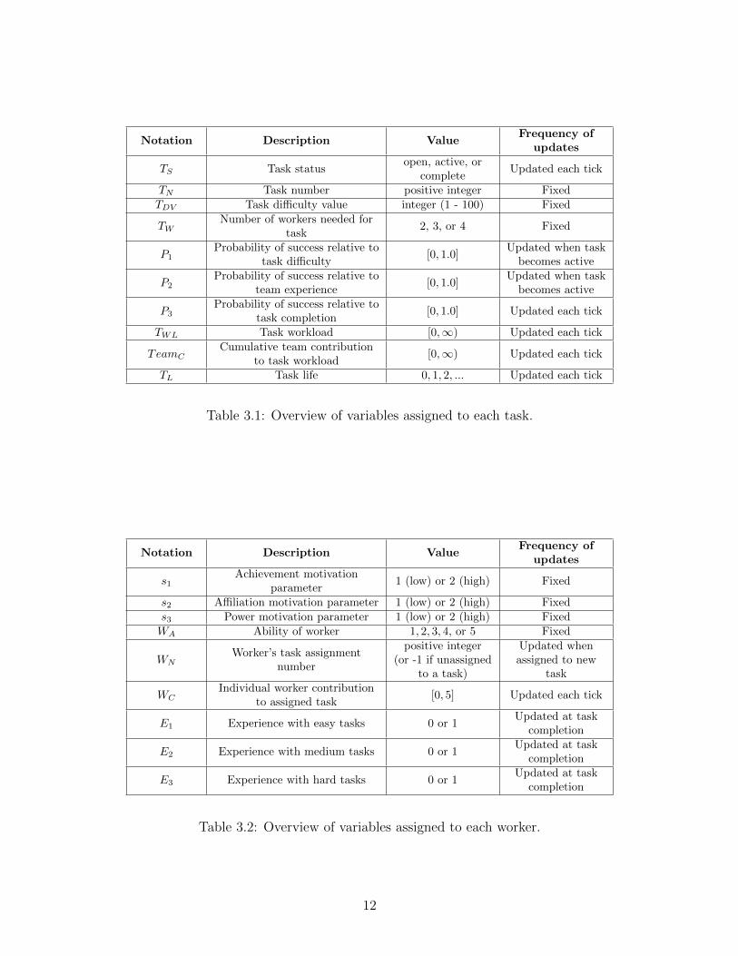
Table 3.1 displays all variables assigned to each task in the model. A task is categorized

by its status (open, active, or complete). A task is open if it has been created but workers

are not yet assigned to the task. A task is active if a team of workers is assigned to the

task and the team is contributing to the task workload. A completed task is a task whose

workload has been fulfilled and no longer has workers assigned to it.

When a task is created, it is assigned a task number (TN

), a di�culty value (TDV

),

and a number of workers (TW

). T

DV

is an integer ranging from 1 to 100 with higher

values indicating a more di�cult task. Number of workers, TW

, is an integer ranging from

2 to 4 and indicates the number of workers that must be assigned to the task before it

becomes active. Both values are randomly chosen for each task from uniform distributions

and do not change during the simulation. Each task is assigned a task life variable (TL

)

that is initialized to zero and incremented by one every time step while the task is active.

Each task is assigned three probability variables P1, P2, and P3 that measure the task’s

probability of success. P1 is determined by the task’s di�culty value, P2 is determined

by the experience levels of workers associated with the task, and P3 is updated at each

time step based on the proximity of a task to its completion. The value of task workload

(TWL

) is determined by the task’s di�culty value and the length of time the task has been

active. Each task has a cumulative team contribution variable (TeamC

) that is updated at

every time step to track progress towards the task’s completion. A task is complete when

Team

C

� T

WL

.

Table 3.2 displays all variables assigned to each worker in the model. The model

10

consists of 100 workers, each of which is characterized by an ability value (WA

) and an

incentive-based motive profile (denoted by s1, s2, s3 in the agent-based model respectively

corresponding to S

ach

, Saff

, and S

pow

from the mathematical model). Each of the motive

profile parameters s1, s2, and s3 has a value of 1 (low) or 2 (high). The ability value

(WA

) is an integer ranging from 1 to 5. Values of s1, s2, s3, and W

A

are selected for each

worker from distributions defined at the initialization of the experiment and do not change

during the simulation. Additionally, each worker has several variables that are updated

at each time step. A worker’s task assignment number is equal to the number of the task

to which the worker is assigned (i.e., WN

= T

N

). If the worker is not currently assigned

to a task, then W

N

is set to �1. Each worker has a worker contribution variable (WC

)

that is updated at each time step and quantifies how much the worker contributes to an

assigned task during the time step. Experience variables E1, E2, and E3 are assigned to

each worker to indicate the worker’s experience with easy, medium, and di�cult tasks,

respectively. The value of an experience variable is 0 initially and updated to 1 when the

worker completes a task with the specified di�culty value.

11

Notation Description Value

Frequency of

updates

TS Task status

open, active, or

complete

Updated each tick

TN Task number positive integer Fixed

TDV Task di�culty value integer (1 - 100) Fixed

TWNumber of workers needed for

task

2, 3, or 4 Fixed

P1Probability of success relative to

task di�culty

[0, 1.0]Updated when task

becomes active

P2Probability of success relative to

team experience

[0, 1.0]Updated when task

becomes active

P3Probability of success relative to

task completion

[0, 1.0] Updated each tick

TWL Task workload [0,1) Updated each tick

TeamCCumulative team contribution

to task workload

[0,1) Updated each tick

TL Task life 0, 1, 2, ... Updated each tick

Table 3.1: Overview of variables assigned to each task.

Notation Description Value

Frequency of

updates

s1Achievement motivation

parameter

1 (low) or 2 (high) Fixed

s2 A�liation motivation parameter 1 (low) or 2 (high) Fixed

s3 Power motivation parameter 1 (low) or 2 (high) Fixed

WA Ability of worker 1, 2, 3, 4, or 5 Fixed

WNWorker’s task assignment

number

positive integer

(or -1 if unassigned

to a task)

Updated when

assigned to new

task

WCIndividual worker contribution

to assigned task

[0, 5] Updated each tick

E1 Experience with easy tasks 0 or 1

Updated at task

completion

E2 Experience with medium tasks 0 or 1

Updated at task

completion

E3 Experience with hard tasks 0 or 1

Updated at task

completion

Table 3.2: Overview of variables assigned to each worker.

12

3.3 Process overview and scheduling

The model begins by creating 100 workers with initial parameters defined in Section 3.5.

Subsequently, one open task is created and randomly assigned T

W

workers (called a team).

Values of P1 and P2 are calculated for the task. This task creation process repeats until

either all of the 100 workers are assigned to tasks or there exists one open task such that

the number of workers needed (TW

) is greater than the number of unassigned workers.

Each task that has been assigned a team is considered an active task.

During each time step, all active tasks are updated one at a time according to the

following procedures. At the beginning of the time step, the value of P3 is updated based

on current values of the task workload (TWL

) and the team’s cumulative contribution to the

task workload (TeamC

). Each worker in the assigned team then calculates it’s individual

worker contribution (WC

). The individual worker contribution values are added to the

cumulative team contribution (TeamC

), TL

is incremented by 1, and the task is checked

for completeness. If a task’s cumulative team contribution is greater than or equal to

the task workload (i.e. TeamC

� T

WL

), the task’s status is changed to ‘complete’ and the

corresponding experience variable (E1, E2, or E3) of each worker in the team is updated. If

a task’s cumulative team contribution is less than the task workload (i.e. TeamC

< T

WL

),

then the task remains active.

At the end of each time step, all workers from completed tasks are unassigned from

their task by setting W

N

= �1 for each of these workers. At the beginning of the next time

step, the task creation process is repeated until either all unassigned workers are assigned

to an open task or there exists one open task such that the number of workers needed (TW

)

is greater than the number of unassigned workers. Therefore, at each time step there will

either be 0 or 1 open tasks. The simulation terminates at the end of 365 time steps.

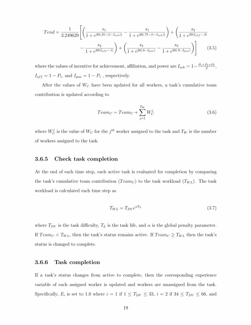
Figure 3.1 shows the history of a single task from its creation to its completion. As

seen in the diagram, the active task loop is repeated until TeamC

� T

WL

.

13

Active Task Loop

Calculate WC for each worker on team and update

TeamC

Create open task and set P1

Assign TW workers to task

Calculate team experience and set P2

Increment TL , update TWL , and compare

TeamC and TWL

when Nt ≥ TW

if TeamC ≥ TWL

Update P3

if task is easy Set E1 = 1.0 for each worker on

team

if task is medium

if task is hard

Update number of completed

tasks and make

all workers on team available

Task Creation Nt = number of available

workers at time t

Task Completion

if TeamC < TWL

Set E2 = 1.0 for each worker on

team

Set E3 = 1.0 for each worker on

team

Figure 3.1: Flow diagram illustrating the history of a single task.

14

3.4 Design concepts

3.4.1 Basic principles

The agent-based model stochastically simulates the proficiency of 100 workers with varying

abilities and motive profiles to complete time-sensitive tasks in small teams over the course

of one year. New tasks are created as workers become available; each new task is randomly

assigned a di�culty value and a team of 2 to 4 workers. Incentive values are associated

with each task based on the task’s probabilities of success. During each time step, each

task workload is updated and workers contribute to their assigned task according to the

mathematical model presented in Section 2.2. At the end of 365 time steps (1 year), the

model outputs the total number of completed tasks, which is the primary measurement

of productivity. By simulating the model hundreds of times for di↵erent sets of initial

distributions and analyzing output, we are able to determine which distributions of worker

motive profiles and abilities lead to increased team-based productivity.

3.4.2 Emergence

The most notable emergent feature of this model is the completion of tasks over time.

A task’s cumulative team contribution variable increases over time as individual workers

contribute to the task. A task is completed when its cumulative team contribution is

greater than or equal to the task workload (i.e. TeamC

� T

WL

).

Another emergent feature of the model is the inability of some teams to complete

assigned tasks. A task workload (TWL

) grows exponentially at a rate determined by the

value of the global penalty parameter ↵. In some cases, a team’s cumulative contribution

(TeamC

) will not increase at a rate needed to surpass (TWL

) over time. In these cases,

Team

C

< T

WL

at every time step and the task will never be completed.

15

3.4.3 Sensing

Each worker knows the task it is currently assigned to and can access the attributes of

this task only. Each task knows which workers are assigned to it and has access to the

attributes of these workers only.

3.4.4 Interaction

Interaction occurs between a task and the workers assigned to it. Workers assigned to a

task contribute to the task workload each time step; the task is complete when the team’s

cumulative contribution equals or exceeds the task workload. When a task is complete,

the experience variables of assigned workers are updated accordingly.

3.4.5 Stochasticity

Values of TDV

and T

W

are randomly assigned to each task from uniform distributions with

ranges specified in Table 3.1. Values of s1, s2, s3, and W

A

are randomly assigned to each

worker from distributions specified at the initialization of the model (see Section 3.5).

3.4.6 Collectives

All workers assigned to the same task form a collective called a team. A team is classified

by its size and the attributes of the team’s workers, including ability, motive profile, and

experience.

3.4.7 Observation

Information about completed tasks is stored at the end of each time step. At the end

of each simulation, output displays the total number of completed tasks which we use as

the primary measure of productivity. Output also displays the average di�culty value,

average life of completed tasks, and the average ability of workers assigned to completed

tasks. These secondary outputs were used for validation and explorative insight, but are

not further discussed in this paper.

16

3.5 Initialization

To initialize the model, the user must specify probability distributions for values of the

motive profile parameters s1, s2, and s3, and a probability distribution for the value of

worker ability W

A

. For example, the user must provide a value of �1 2 [0, 1] such that

Prob(s1 = 1.0) = �1 and Prob(s1 = 2.0) = 1� �1. Similarly, values of �2 and �3 must also

be provided. The user must also specify values of i

2 [0, 1] for i = 1, 2, 3, 4, 5 such thatP5

i=1 i

= 1. These values determine the ability distribution where P (WA

= i) = i

for

i = 1, 2, 3, 4, 5.

The value of ↵ must also be specified at the model’s initialization. The global penalty

parameter ↵ is used by all tasks to calculate current workload according to the equation

T

WL

= T

DV

e

↵T

L where T

DV

is the task di�culty value and T

L

is the task life. To ensure a

20% increase in T

WL

occurs after t = 14 time steps (i.e. 2 weeks), we chose ↵ = ln(1.2)14 .

3.6 Submodels

3.6.1 P

1

calculation

P1 measures a task’s probability of success based on its di�culty value. It is assumed that

easy tasks have a high probability of success and di�cult tasks have a low probability of

success. Accordingly, the value of P1 is calculated for each task as

P1 =100� T

DV

100(3.1)

where T

DV

is the task di�culty value.

3.6.2 Team experience and P

2

calculation

All workers assigned to the same task have an experience variable E

i

where i = 1 if

1 T

DV

33, i = 2 if 34 T

DV

66, and i = 3 if 67 T

DV

100. A worker is either

considered experienced if Ei

= 1 or inexperienced if Ei

= 0. The team’s experience value

17

for the assigned task is calculated as

E =1

T

W

T

WX

j=1

E

j

i

(3.2)

where E

j

i

is the value of Ei

for the j

th worker assigned to the task, and T

W

is the number

of workers assigned to the task.

P2 measures a task’s probability of success relative to the experience of its team and

is set equal to E. Therefore, if all workers assigned to the task are experienced, then

P2 = 1.0. If all workers assigned to the task are inexperienced, then P2 = 0. Otherwise,

0 < P2 < 1.0.

3.6.3 P

3

calculation

P3 measures a task’s probability of success relative to its proximity to being complete.

Hence, at the beginning of each time step, P3 is evaluated as

P3 =Team

C

T

WL

(3.3)

where Team

C

is the task’s cumulative team contribution and T

WL

is the task workload.

3.6.4 Worker and team contributions to a task

For each task, the contribution of an assigned worker is denoted by W

C

and is updated

each time step using the formula

W

C

= Tend ·WA

(3.4)

where Tend is the worker’s tendency to contribute to the task and W

A

is worker’s ability.

As described in Section 2.2, the value of Tend depends on the worker’s motive profile and

the task’s incentive value according to

18

Tend =1

3.249629

"✓s1

1 + e

20(.25�(1�I

ach

))� s1

1 + e

20(.75�(1�I

ach

))

◆+

✓s2

1 + e

20(Iaff

�.3)

� s2

1 + e

20(Iaff

�.1)

◆+

✓s3

1 + e

20(.6�I

pow

)� s3

1 + e

20(.9�I

pow

)

◆#(3.5)

where the values of incentive for achievement, a�liation, and power are Iach

= 1� P1+P2+P33 ,

I

aff

= 1� P1, and I

pow

= 1� P1 , respectively.

After the values of WC

have been updated for all workers, a task’s cumulative team

contribution is updated according to

Team

C

= Team

C

+T

WX

j=1

W

j

C

(3.6)

where W j

C

is the value of WC

for the jth worker assigned to the task and T

W

is the number

of workers assigned to the task.

3.6.5 Check task completion

At the end of each time step, each active task is evaluated for completion by comparing

the task’s cumulative team contribution (TeamC

) to the task workload (TWL

). The task

workload is calculated each time step as

T

WL

= T

DV

e

↵T

L (3.7)

where TDV

is the task di�culty, TL

is the task life, and ↵ is the global penalty parameter.

If TeamC

< T

WL

, then the task’s status remains active. If TeamC

� T

WL

then the task’s

status is changed to complete.

3.6.6 Task completion

If a task’s status changes from active to complete, then the corresponding experience

variable of each assigned worker is updated and workers are unassigned from the task.

Specifically, Ei

is set to 1.0 where i = 1 if 1 T

DV

33, i = 2 if 34 T

DV

66, and

19

i = 3 if 67 T

DV

100. The task assignment variable, WN

, for each worker assigned to

the completed task is set to �1.

3.7 Implementation

The model was coded in NetlLogo (Version 6.0) [22]. This software has a unique program-

ming language and customizable interface that is designed specifically for ABM develop-

ment and implementation. NetLogo has an important tool called BehaviorSpace that was

used to simulate variations of populations under di↵erent parameters. Statistical analyses

and graphical displays were conducted in R [14].

20

Chapter 4

Results

4.1 Impact of motivation on productivity

We first investigated how the total number of completed tasks varies for di↵erent motive

profile distributions. Each motive profile distribution is described by the values of �1, �2,

and �3 where P (si

= 2.0) = �

i

and P (si

= 1.0) = 1 � �

i

for i = 1, 2, 3. For each of the

27 di↵erent motive profile distributions in Table 4.1, we simulated the model and collected

output 100 times. In all of these simulations, the values of worker ability (WA

) were chosen

randomly from a uniform distribution.

Figure 4.1 displays box plots summarizing the total number of tasks completed over 100

simulations for each motive profile parameter set. In these simulations, task di�culty values

range from 1 to 100. The motive profile parameter sets are numbered in order of descending

value for the mean number of completed tasks. Thus, parameter set 1 (�1 = �2 = �3 = 0.75)

corresponds to the motive profile distribution that yields the greatest number of completed

tasks on average. The average number of completed tasks observed with parameter set 1

is 653.52, which is a 44.5% increase over the average number of completed tasks observed

with motive profile parameter set 14. Parameter set 14 corresponds to the baseline scenario

in which all workers are equally likely to have high or low values in each motivation type

(�1 = �2 = �3 = 0.50) .

21

Parameter �1 �2 �3

Set P (s1 = 2.0) P (s2 = 2.0) P (s3 = 2.0)1 0.75 0.75 0.752 0.75 0.50 0.753 0.75 0.75 0.504 0.75 0.25 0.755 0.75 0.50 0.506 0.75 0.25 0.507 0.50 0.75 0.758 0.75 0.75 0.259 0.75 0.50 0.2510 0.50 0.50 0.7511 0.50 0.75 0.5012 0.75 0.25 0.2513 0.50 0.25 0.7514 0.50 0.50 0.5015 0.50 0.75 0.2516 0.50 0.25 0.5017 0.25 0.75 0.7518 0.25 0.50 0.7519 0.50 0.50 0.2520 0.50 0.25 0.2521 0.25 0.25 0.7522 0.25 0.75 0.5023 0.25 0.50 0.5024 0.25 0.75 0.2525 0.25 0.25 0.5026 0.25 0.50 0.2527 0.25 0.25 0.25

Table 4.1: Parameter sets defining each of the 27 di↵erent motive profile distributions.

22

Figure 4.1: Statistical summary of the number of completed tasks from 100 model simula-tions for each motive profile distribution. Task di�culty values range from 1 to 100.

Motive profile parameter sets 1 through 6 correspond to the motive profile distributions

that yielded the highest values of productivity on average. These six parameter sets have

one thing in common; they all assume the probability of selecting a worker with high

achievement motivation is maximized (i.e. �1 = 0.75). Values of �2 vary between 0.75 and

0.25, while values of �3 vary between 0.75 and 0.50 in these six motive profile parameter

sets. These results suggests that if task di�culty values span the full range (1 to 100)

then hiring workers with high achievement motivation should be a top priority in order to

maximize productivity.

It is also worth noting that motive profile parameter sets 15, 17, 18, 21, 22, and 24

all include �2 = 0.75 and/or �3 = 0.75, but these sets do not correspond to high produc-

tivity. These five parameters sets maximize the probability of selecting workers with high

a�liation motivation, or high power motivation, or both (as seen in parameter set 17).

However, each of these parameter sets yields an average number of completed tasks that

is less than that of the baseline scenario. This result indicates that if task di�culty values

span the full range (1 to 100) then hiring workers with high motivation of any type is

not su�cient to maximize productivity. Furthermore, profile parameter set 17 highlights

the impact of achievement motivation on productivity, since despite this parameter set

23

including �2 = �3 = 0.75 the average number of completed tasks that is less than that of

the baseline scenario due to �1 = 0.25.

To further explore the impact of motive profiles on productivity, we repeated the above

experiment using model simulations with only hard tasks (67 T

DV

100) and model

simulations with only easy tasks (1 T

DV

33). Figure 4.2 displays box plots corre-

sponding to the motive profile parameter sets that perform better than the baseline set

(parameter set 14). When all tasks are di�cult (Figure 4.2 A), the three best motive

profile parameter sets (4, 2, and 1) correspond to those having �1 = 0.75 and �3 = 0.75.

This result suggests that, in situations where tasks are consistently di�cult, it is important

to hire workers with high power motivation in addition to high achievement motivation.

When all tasks are easy (Figure 4.2 B), the three best motive profile parameter sets (3, 8,

and 1) correspond to those having �1 = 0.75 and �2 = 0.75. In fact, the first six parameter

sets in Figure 4.2 B correspond to those with �2 = 0.75. This result suggests that, in

situations where tasks are consistently easy, hiring workers with high a�liation motivation

should be a top priority in order to maximize productivity.

24

Figure 4.2: Statistical summary of the number of completed tasks from 100 model simu-lations for each of the top performing motive profile distributions. Top: Panel A displaysresults obtained with simulations using task di�culty values between 67-100. Bottom:Panel B displays results obtained with simulations using task di�culty values between1-33.

25

4.2 Impact of ability on productivity

We next investigated how the total number of completed tasks varies for di↵erent ability

distributions. Each ability distribution is described by the values of 1, 2, 3, 4, and

5 where P (WA

= j) =

j

for j = 1, 2, 3, 4, 5. We considered five di↵erent ability dis-

tributions (Table 4.2): two bimodal distributions (parameter sets A and D), two normal

distributions (parameter sets C and E), and one uniform distribution (parameter set B).

All ability parameter sets have a distribution mean value of 3. For each of these five abil-

ity distributions, we simulated the model and collected output 100 times. In all of these

simulations, motive profiles were selected from the distribution defined by parameter set 1

in Table 4.1.

Figure 4.3 displays box plots summarizing the total number of tasks completed over

100 simulations for each ability distribution. In these simulations, task di�culty values

range from 1 to 100. The ability parameter sets are lettered in order of descending value

for the mean number of completed tasks. Thus, parameter set A corresponds to the ability

distribution that yields the greatest number of completed tasks on average. The average

number of completed tasks observed with the ability distribution defined by parameter

set A is 730.61, which is an 11.8% increase over the average number of completed tasks

observed with the ability distribution defined by parameter set B. Parameter set B defines

the uniform ability distribution and corresponds to the ability distribution used in the

experiments in Section 4.1.

The average number of completed tasks observed with each of the ability distributions

decreases as the value of 5 decreases. The average number of completed tasks is at its

smallest when the ability distribution defined by parameter set E is implemented. Param-

eter set E assumes all workers have ability 2, 3, or 4. Hence, the corresponding distribution

has no workers with ability 5. On the other hand, the most productive distribution, defined

by parameter set A, corresponds to the bimodal ability distribution classifying workers as

having either ability 1 or 5 with equal probability. Parameter set A assumes all workers

have the highest ability or the lowest ability value. These results highlight the value of

high-ability workers in maximizing productivity, and suggest hiring as many high ability

26

workers as possible even if it results in the remaining workers having low ability.

Parameter 1 2 3 4 5

Set P (WA

= 1) P (WA

= 2) P (WA

= 3) P (WA

= 4) P (WA

= 5)A 0.50 0.0 0.0 0.0 0.50B 0.20 0.20 0.20 0.20 0.20C 0.10 0.20 0.30 0.20 0.10D 0.0 0.50 0.0 0.50 0.0E 0.0 0.30 0.40 0.30 0.0

Table 4.2: Parameter sets defining each of the five di↵erent ability distributions.

Figure 4.3: Statistical summary of the number of completed tasks from 100 model simula-tions for each ability distribution. Task di�culty values range from 1 to 100. The motiveprofile distribution is defined by parameter set 1 in Table 4.1.

27

4.3 Task Failure Detection

In the model, it is possible for an active task to never be completed during a simulation if

the task workload (TWL

) increases faster than the team’s cumulative contribution (TeamC

).

These are called failing tasks. In all of the model experiments discussed thus far, failing

tasks remain active until the end of the simulation and the assigned team continues to

contribute to the task even though it is impossible for the team complete the task.

To mitigate the negative impact of failing tasks on productivity, we designed a model

feature called Task Failure Detection (TFD). During the simulation, TFD assesses whether

a task is failing or not and allows for a new team of workers to be assigned to failing tasks

as they are identified. At every time step, TFD assesses each task by comparing the current

value of Team

C

T

WL

to the value obtained during the previous time step. If it is the case that

✓Team

C

T

WL

◆

i�1

>

✓Team

C

T

WL

◆

i

(4.1)

where i denotes the tick, then the task is deemed a failing task. If inequality (4.1) holds true

for at least one time step i, then it remains true at all subsequent time steps and Team

C

<

T

WL

for the entire simulation. This is due to the fact that TWL

grows exponentially with

time while Team

C

increases by an additive amount each time step. Thus, inequality 4.1

is an accurate indicator of a failing task. Once a task is marked as failing, the workers are

immediately removed from this task. The task is randomly assigned a new team of workers

when they become available.

Figure 4.4 displays box plots summarizing the total number of tasks completed over

100 simulations with TFD and without TFD. In these simulations, task di�culty values

range from 1 to 100. The motive profile of each worker is selected from the distribution

defined by parameter set 1 and the ability of each worker is selected from the distribution

defined by parameter set A. On average, the number of completed tasks in simulations with

TFD is 838.71, which is a 14.8% increase over the average number of completed tasks in

simulations without TFD. These results suggest that evaluating task progress on a frequent

basis and reassigning a new team to a failing task can substantially increase productivity.

28

Figure 4.4: Statistical summary of the number of completed tasks from 100 model simula-tions with TFD and without TFD. Task di�culty values range from 1 to 100. The motiveprofile distribution is defined by parameter set 1. The ability distribution is defined byparameter set A.

29

Chapter 5

Conclusions

In this thesis, we present one framework for evaluating optimal hiring guidelines for a

team-based organization based on the abilities and motivational preferences of workers.

Our agent-based model (ABM) can be easily modified to accommodate organizations of

any size and tasks that range between any di�culty values. The ABM o↵ers the flexibil-

ity of simulating team-based dynamics over any time frame and under any set of initial

conditions. The main use of the ABM is to compare productivity across di↵erent pools of

workers and quantify the impact of hiring workers with certain attributes.

In the experiments presented here, we found that both motivational profiles and abil-

ity substantially impact productivity in a team-based organization. In experiments that

included tasks of all di�culty values, we found that the optimal distribution of motive

profiles among workers can increase productivity by 44.5% on average compared to base-

line values. Furthermore, when the optimal distribution of ability values was implemented,

average productivity increased by an additional 11.8%. These results suggest that both

characteristics (ability and motive profile) should be considered during the hiring process.

The results highlighted in this thesis are dependent upon the di�culty of the organiza-

tion’s essential tasks. Our framework requires an organization’s essential tasks be defined

by di�culty values ranging from 1 to 100. When di�culty values span the entire range,

our results shows that hiring workers with high achievement motivation is critical to max-

imizing productivity. When tasks were limited to only di�culty tasks, we observed a need

30

for workers with both high achievement and power motivation. This was di↵erent from

the results found when only easy tasks were considered. In this case, the optimal results

suggest hiring practices prioritize selecting workers with high a�liation motivation.

In working with the model we noticed some tasks remained incomplete for the dura-

tion of the simulation due to an underperforming team. In looking more closely at the

properties of these tasks, we realized these tasks could be recognized in real-time. We

developed a new model feature to recognize failing tasks as they emerge and immediately

re-assign a new team of workers to the failing task. By implementing this new feature, we

found a 14.8% increase in average productivity at the organizational level. This feature

is not only important to maximizing productivity, but it is also important to maximizing

worker motivation. A worker assigned to a failing task will exhibit decreasing tendencies

to contribute to their work, which is a sign of an unmotivated employee.

Future work includes conducting a sensitivity analysis to determine which of the model

parameters have the greatest impact on our results. Parameters such as the number of

workers, the size of the teams, and the penalty value will be investigated. Other parameters

to investigate include the parameters defining the motive profiles, specifically the gradients

and turning points to approach or avoidance. Additionally, in the future we will use the

model to investigate scenarios of dynamic parameter perturbation during simulation under

known conditions. One such scenario involves introducing a worker (or group of work-

ers) with known attributes that are vastly di↵erent from other workers into the system

to observe outcomes that deviate from expected results. It is also possible for us to con-

sider implementing variations in the organizational structure (e.g. employee participation

programs) that might better represent certain sectors of industry.

31

Bibliography

[1] Bartel, A. P. (1994). Productivity gains from the implementation of employee training

programs. Industrial Relations, 33, 411-425.

[2] Becker, B. E., & Huselid, M. A. (1992). Direct estimates of SD sub y and the impli-

cations for utility analysis. Journal of Applied Psychology, 77, 227-233.

[3] Bowen, D. E. Ledford Jr., G. E. & Nathan, B. R. (1991, Nov). The Executive, 5 (4),

35-51. Academy of Management.

[4] Delaney, J. T., & Huselid, M. A. (1996). The impact of human resource manage-

ment practices on perceptions of organizational performance. Academy of Management

Journal, 39 (4), 949.

[5] Gerhart, B., & Milkovich, G. T. (1992). Employee compensation: Research and prac-

tice. In M. D. Dunnette & L. M. Hough (Eds.), Handbook of industrial and organiza-

tional psychology, 3, 481-569. Palo Alto, CA: Consulting Psychologists Press.

[6] Heckhausen, J., & Heckhausen, H. (2008). Motivation and action. New York: Cam-

bridge University Press.

[7] Knoke, D., & Kalleberg, A. L. (1994). Job training in U.S. organizations. American

Sociological Review, 59, 537-546.

[8] Levine, D. I. (1995). Reinventing the workplace: How business and employees can both

win.Washington, DC: Brookings Institution.

[9] McClelland, D. C. (1961). The achieving society Princeton, N.J., Van Nostrand.

32

[10] McClelland, D. C. (1975). Power: the inner experience. New York: Irvington.

[11] Merrick K, Shafi, K. (2011) Achievement, a�liation, and power: Motive profiles for

artificial agents. Adaptive Behavior, 19 (1), 40-62.

[12] Ormrod, J.E. (2004). Human Learning (4th ed.). Upper Saddle River, NJ: Pearson.

[13] Osterman, P. (1987). Choice of employment systems in internal labor markets. Indus-

trial Relations, 26, 46-57.

[14] R Core Team (2013). R: A language and environment for statistical computing. R

Foundation for Statistical Computing, Vienna, Austria.

[15] Railsback SF, Grimm V. (2012). Agent-Based and Individual-Based Modeling. Prince-

ton, NJ: Princeton University Press.

[16] Russell, J. S., Terborg, J. R., & Powers, M. L. (1985). Organizational performance

and organizational level training and support. Personnel Psychology, 38, 849-863.

[17] Schmidt, F. L., Hunter, J. E., McKenzie, R. C., & Muldrow, T. W. (1979). Impact of

valid selection procedures on work-force productivity. Journal of Applied Psychology,

64, 609-626.

[18] Schreiber, J. B. (2016). Motivation 101. Springer Publishing Company.

[19] Starfield, A. M. Smith, K.A. & Bleloch, A. L. (1990). How to model it: Problem solving

for the computer age. McGraw-Hill, New York.

[20] Wagner, J. A. (1994). Participation’s e↵ect on performance and satisfaction: A recon-

sideration of research evidence. Academy of Management Review, 19, 312-330.

[21] Wickham, H. (2011). The Split-Apply-Combine Strategy for Data Analysis. Journal

of Statistical Software, 40 (1), 1-29.

[22] Wilensky, U. (1999). NetLogo [Computer software]. Retrieved from

http://ccl.northwestern.edu/netlogo/.

33