a condition based maintenance approach to forecasting b-1
TRANSCRIPT

Air Force Institute of TechnologyAFIT Scholar
Theses and Dissertations Student Graduate Works
3-23-2017
A Condition Based Maintenance Approach toForecasting B-1 Aircraft PartsJoshua D. DeFrank
Follow this and additional works at: https://scholar.afit.edu/etd
Part of the Operations and Supply Chain Management Commons
This Thesis is brought to you for free and open access by the Student Graduate Works at AFIT Scholar. It has been accepted for inclusion in Theses andDissertations by an authorized administrator of AFIT Scholar. For more information, please contact [email protected].
Recommended CitationDeFrank, Joshua D., "A Condition Based Maintenance Approach to Forecasting B-1 Aircraft Parts" (2017). Theses and Dissertations.793.https://scholar.afit.edu/etd/793

A CONDITION BASED MAINTENANCE APPROACH TO FORECASTING B-1
AIRCRAFT PARTS
THESIS
Joshua D. DeFrank, Captain, USAF
AFIT-ENS-MS-17-M-123
DEPARTMENT OF THE AIR FORCE AIR UNIVERSITY
AIR FORCE INSTITUTE OF TECHNOLOGY
Wright-Patterson Air Force Base, Ohio
DISTRIBUTION STATEMENT A.
APPROVED FOR PUBLIC RELEASE; DISTRIBUTION UNLIMITED.

The views expressed in this thesis are those of the author and do not reflect the official
policy or position of the United States Air Force, Department of Defense, or the United
States Government. This material is declared a work of the U.S. Government and is not
subject to copyright protection in the United States.

AFIT-ENS-MS-17-M-123
A CONDITION BASED MAINTENANCE APPROACH TO FORECASTING B-1
AIRCRAFT PARTS
THESIS
Presented to the Faculty
Department of Operational Sciences
Graduate School of Engineering and Management
Air Force Institute of Technology
Air University
Air Education and Training Command
In Partial Fulfillment of the Requirements for the
Degree of Master of Science in Logistics and Supply Chain Management
Joshua D. DeFrank, BS, MBA
Captain, USAF
March 2017
DISTRIBUTION STATEMENT A.
APPROVED FOR PUBLIC RELEASE; DISTRIBUTION UNLIMITED.
AFIT-ENS-MS-17-M-123
A CONDITION BASED MAINTENANCE APPROACH TO FORECASTING B-1
AIRCRAFT PARTS
Joshua D. DeFrank, BS, MBA
Captain, USAF
Committee Membership:
Capt Michael P. Kretser, PhD
Chair
Dr. Alan W. Johnson
Co-Advisor

iv
AFIT-ENS-MS-17-M-123
Abstract
United States Air Force (USAF) aircraft parts forecasting techniques have
remained archaic despite new advancements in data analysis. This approach resulted in a
57% accuracy rate in fiscal year 2016 for USAF managed items. Those errors combine
for $5.5 billion worth of inventory that could have been spent on other critical spare
parts. This research effort explores advancements in condition based maintenance (CBM)
and its application in the realm of forecasting. It then evaluates the applicability of CBM
forecast methods within current USAF data structures. This study found large gaps in
data availability that would be necessary in a robust CBM system. The Physics-Based
Model was used to demonstrate a CBM like forecasting approach on B-1 spare parts, and
forecast error results were compared to USAF status quo techniques. Results showed the
Physics-Based Model underperformed USAF methods overall, however it outperformed
USAF methods when forecasting parts with a smooth or lumpy demand pattern. Finally,
it was determined that the Physics-Based Model could reduce forecasting error by 2.46%
or $12.6 million worth of parts in those categories alone for the B-1 aircraft.

v
For God, Family, and Country

vi
Acknowledgments
I would like to express my sincere appreciation to my advisors. To Dr. Alan
Johnson for his sage advice, breadth of knowledge, and many connections which were
foundational in helping me put together the elements of this work. To Dr. Michael
Kretser, whose forecasting expertise and maintenance acumen was especially influential
in helping me navigate which research paths to explore.
Additionally, I would like to thank several other professors who have spent
quality time educating me. Dr. Jason Freels taught me the fundamentals of analyzing
reliability statistical data, and Dr. Daniel Steeneck revolutionized my view on condition
based maintenance forecasting techniques.
A mentor of mine often said, “Logistics is a team sport.” Through this experience,
I have learned that research is too. For that, I am also indebted to many people from
multiple organizations who helped me on this journey. To the researchers at the Logistics
Management Institute who connected me with the original Physics-Based Model and who
willingly shared many other of their research efforts (Dr. Brad Silver, Dr. David
Peterson, Steve Long, Ward “Skip” Tyler). To Dr. Marvin Arostegui who gladly helped
me obtain the D200 forecast data necessary for this research. Joshua Moore (420 SCMS)
was critical in helping me understand how the Air Force forecasting process works.
Chief Joseph Sternod was pivotal in helping me categorize B-1 parts as well as
understand how we can collect better data for future efforts. Finally, to John Rusnak and
Bill Donaldson from HAF/A4P and Mr. Don Lucht at AFMC/A4P for sponsoring this
research.
Josh DeFrank
vii
Table of Contents
Page
Abstract .............................................................................................................................. iv
Acknowledgments.............................................................................................................. vi
Table of Contents .............................................................................................................. vii
List of Figures ......................................................................................................................x
List of Tables ..................................................................................................................... xi
List of Equations ............................................................................................................... xii
I. Introduction ......................................................................................................................1
Background .....................................................................................................................1 Problem Statement ..........................................................................................................4
Investigative Questions ...................................................................................................5 Research Focus................................................................................................................5 Methodology ...................................................................................................................6
Assumptions and Limitations ..........................................................................................6 Significance of Research .................................................................................................7
What to Expect ................................................................................................................7
II. Literature Review ............................................................................................................9
Chapter Overview ...........................................................................................................9 USAF Forecasting ...........................................................................................................9
USAF Forecast Accuracy ........................................................................................ 12 Demand Forecast Accuracy .................................................................................... 14
Replacement Parts Forecasting .....................................................................................15 Alternative USAF Forecasting Models .........................................................................18 CBM Philosophy ...........................................................................................................22
Diagnostics/Prognostics .......................................................................................... 22 Event Data ............................................................................................................... 23
Condition Monitoring Data ..................................................................................... 23 CBM+ in DoD ...............................................................................................................24
CBM Forecast Methods ................................................................................................30 Summary .......................................................................................................................33
III. Methodology ................................................................................................................34
Chapter Overview .........................................................................................................34 PBM Basics ...................................................................................................................34
viii
Flying Hours (FH) .................................................................................................. 34
Cold Cycles (CC) .................................................................................................... 35 Warm Cycles (WC) .................................................................................................. 35 Ground Cycles (GC) ................................................................................................ 35
Model Mean and Variance ...................................................................................... 36 Model Assumptions ................................................................................................. 36 Model Calibration: Maximum Likelihood Estimation ............................................ 37 Sliding Scale ............................................................................................................ 38
Data ...............................................................................................................................39
Sources .................................................................................................................... 39 Data Cleaning and Filtering Selected NIINs .......................................................... 40 Demand Patterns ..................................................................................................... 42 Slow Trends ............................................................................................................. 43
USAF Forecast Method ................................................................................................44 Experiments...................................................................................................................45
Test #1. Mechanical versus Electrical Forecasting Accuracy ................................ 45 Test #2. Demand Pattern Comparison .................................................................... 46
Forecast Error ......................................................................................................... 46 Comparative Statistics ............................................................................................. 46
Conclusion ....................................................................................................................48
IV. Analysis and Results ....................................................................................................49
Chapter Overview .........................................................................................................49
Investigative Question 1 ................................................................................................49
Investigative Question 2 ................................................................................................50
Investigative Question 3 ................................................................................................51 Investigative Question 4 ................................................................................................51
Summary Statistics ........................................................................................................52 Assumptions ..................................................................................................................52 Test #1. Mechanical versus Electrical Forecasting Accuracy .......................................53
Test #2. Demand Pattern Comparison ..........................................................................57 Smooth ..................................................................................................................... 57
Lumpy ...................................................................................................................... 58 Intermittent .............................................................................................................. 59
Erratic ..................................................................................................................... 60 Overall Demand Pattern Comparison .................................................................... 61
Summary .......................................................................................................................65
V. Conclusions and Recommendations .............................................................................67
Chapter Overview .........................................................................................................67 Conclusions of Research ...............................................................................................67 Significance of Research ...............................................................................................69
Recommendations for Action .......................................................................................70 Recommendations for Future Research ........................................................................71
ix
Recommendation 1: Potential conditional information sources ............................. 71
Recommendation 2: CBM Inventory Policy ............................................................ 72 Recommendation 3: PBM Sliding Scale Analysis ................................................... 72
Summary .......................................................................................................................73
Appendix A: Weapon Systems Dash Board ......................................................................74
Appendix B: Diagnostic and Prognostic CBM Summary .................................................75
Appendix C: Sliding Scale Equations ................................................................................76
Appendix D: Demand Pattern Demand Data .....................................................................77
Appendix E: Mechanical and Electrical Demand Data .....................................................78
Appendix F: Quad Chart ....................................................................................................79
Bibliography ......................................................................................................................80

x
List of Figures
Page
Figure 1: CBM+ Future State (Navarra et al., 2007) .......................................................... 2
Figure 2: USAF OIM Forecast Method ............................................................................ 11
Figure 3: Hierarchy of Forecasting Methods (Lowas III, 2015) ....................................... 16
Figure 4: Proportional Flying Hour Model Vs. Sortie Model (Slay, 1995) ...................... 19
Figure 5: Operation Desert Storm C-5 Analysis (Wallace et al., 2000) ........................... 21
Figure 6: Affinity Diagram of CBM Data Warehouse Components (Henderson & Kwinn,
2005) .......................................................................................................................... 29
Figure 7: Demand Pattern Matrix (Lowas III, 2015) ........................................................ 42
Figure 8: B-1 Demand Pattern Frequency ........................................................................ 52
Figure 9: Multicollinearity Test ........................................................................................ 53
Figure 10: PBM Forecast Error Relative to Non-Transformed 8QMA ............................ 64
Figure 11: Non-Transformed Versus Transformed Forecast Accuracy ........................... 64
Figure 12: Lumpy Forecast Error ..................................................................................... 65
Figure 13: December 2016 Operations Summary Snapshot ............................................. 74

xi
List of Tables
Page
Table 1: Smooth Structural NIINs and Associated Forecasting Accuracies (Lowas III,
2015) .......................................................................................................................... 14
Table 2: Mission Type Impact on Langley F-15C/D Parts Demand (Slay & Sherbrooke,
1997) .......................................................................................................................... 20
Table 3: FSC Classifications ............................................................................................. 54
Table 4: Test #1 Forecast Error Results ............................................................................ 55
Table 5: Aggregate MASE by Part Category ................................................................... 56
Table 6: F-Test for Equal Variances ................................................................................. 56
Table 7: Test for Equal Means .......................................................................................... 56
Table 8: Smooth Demand Forecasts ................................................................................. 58
Table 9: Lumpy Demand Forecasts .................................................................................. 59
Table 10: Intermittent Demand Forecasts ......................................................................... 60
Table 11: Erratic Demand Forecasts ................................................................................. 61
Table 12: Demand Pattern Comparison ............................................................................ 62
Table 13: Smooth Demand F-Test for Equal Variances ................................................... 62
Table 14: Smooth Demand Test for Equal Means ............................................................ 62
Table 15: Lumpy Demand F-Test for Equal Variances .................................................... 63
Table 16: Lumpy Demand Test for Equal Means ............................................................. 63

xii
List of Equations
Page
Equation 1: Demand Forecast Accuracy........................................................................... 14
Equation 2: Proportional Hazards Model ......................................................................... 30
Equation 3: Model Mean .................................................................................................. 36
Equation 4: Model Variance ............................................................................................. 36
Equation 5: Likelihood Function ...................................................................................... 37
Equation 6: Conditional Likelihood Function .................................................................. 37
Equation 7: Log-Likelihood Function .............................................................................. 37
Equation 8: Maximum Likelihood Function..................................................................... 38
Equation 9: Total OIM Demand ....................................................................................... 40
Equation 10: Average Demand Interval ........................................................................... 43
Equation 11: Coefficient of Variation............................................................................... 43
Equation 12: First Shear Transformation .......................................................................... 44
Equation 13: Second Shear Transformation ..................................................................... 44
Equation 14: Eight Quarter Moving Average ................................................................... 44
Equation 15: Mean Absolute Scaled Error………………………………………………46
Equation 16: Difference between Means Confidence Interval ......................................... 47

1
A CONDITION BASED MAINTENANCE APPROACH TO
FORECASTING B-1 AIRCRAFT PARTS
I. Introduction
Background
As technology advances, it should follow that forecasting techniques will advance
as well. However, aircraft parts forecasting practices for the United States Air Force
(USAF) have remained archaic, resulting in a 57% accuracy rate in fiscal year 2016 for
USAF managed items. The error from this approach inhibited $5.5 billion worth of
inventory from being repurposed toward other USAF priorities. This research effort
explores advancements in condition based maintenance (CBM) research, and specifically
its application in the realm of forecasting. Then it will evaluate the applicability of those
forecast methods within current USAF data structures. The Physics-Based Model will be
used to demonstrate a CBM-like forecasting approach, and error results will be compared
to USAF baseline procedures.
CBM is not a new concept for the USAF. In 2002, the Deputy Under Secretary of
Defense for Logistics and Material Readiness directed the military to develop and
implement Condition Based Maintenance Plus (CBM+). This directive defined CBM as
“a set of maintenance processes and capabilities derived from real-time assessment of
weapon system condition obtained from embedded sensors and/or external test and
measurements using portable equipment” (Smith, 2003). The annotation of “CBM+” that
is unique to the military services is signaling the integration of technologies and
processes, with the aim of improving system effectiveness (Under Secretary of Defense

2
for Acquisition Technology and Logistics, 2012). CBM+ could be further explained as
CBM that is enhanced by reliability analysis and prognostic capabilities. However, it
should be noted that other sources include this aspect as an inherent aspect of CBM, as
will be discussed later (Jardine, Lin, & Banjevic, 2006).
Furthermore, the CBM+ initiative was an integral part of the Expeditionary
Logistics for the 21st Century (eLog21) campaign. This movement sought to implement
the systems and processes in place that would enable Agile Combat Support, one of the
six core competencies of the USAF (Navarra, Lawton, McCusker, & Hearrell, 2007). The
main goal behind moving toward CBM+ was to improve maintenance agility and
responsiveness, to increase operational availability, and to reduce lifecycle total
ownership costs (Navarra et al., 2007). In order to do this, it was recognized that
Information Technology (IT) systems and processes would need to be redesigned around
this new concept. A future state model of the IT system that a CBM+ program would
necessitate is shown in Figure 1.
Figure 1: CBM+ Future State (Navarra et al., 2007)

3
The Expeditionary Combat Support System was the program undertaking this immense
responsibility. However, when that program was discontinued in 2012, CBM+ in the
USAF essentially died as well.
USAF methodology for maintenance and supply support is based on engineering
and decades of refined practice. Traditional USAF maintenance practices are founded on
technical order instructions, which specify when and how to perform maintenance
actions. This methodology fits under preventative maintenance practices (L. Swanson,
2001). Generally speaking, maintenance actions are completed on fixed time or use
intervals, precluding hard part failures. This method is imprecise and frequently results in
disposing parts long before reaching the end of their useful life (Ellis, 2008). The USAF’s
demand forecasting techniques have evolved over the years, however still primarily rely
on historic demand (Bachman, 2007).
The USAF uses a variety of forecasting techniques, however the primary method
used is an eight quarter moving average. This method is used in over 80% of occurrences.
Details of this as well as other USAF techniques will be elaborated on in Chapter II.
While these practices have been adequate for the USAF, the Chief of Staff, General
Goldfein stressed in a recent newsletter that "Air and Space superiority are not American
birthrights" (Goldfein, 2017). He went on to describe that the USAF is at a pivotal
moment where its superiority gap over other nation’s air forces is diminishing, and in
some cases has already closed. Readiness is a term frequently used to describe the
USAF’s state of preparedness to engage in warfare. Often readiness is measured by the
rate of aircraft availability. The only component of aircraft availability that pertains to
spare parts is the Total Non-Mission Capable for Supply (TNMCS). A snapshot taken of

4
December 2016’s supply performance shows that 18 of 39 (46%) weapon systems did not
meet their TNMCS standard for the month (Appendix A: Weapon Systems Dash Board).
This metric tells us that the USAF supply chain does not deliver the supply support it is
programmed to provide. It is the hope that by studying new demand forecasting
techniques that the USAF can improve its supply performance and thereby reduce the
amount of aircraft not meeting their respective TNMCS standards.
The need for better processes is clear to see within the USAF. As CBM is still a
relatively new maintenance philosophy, the pressing challenge is to unlock the benefit
from behind what conditional data can provide. According to Greitzer et al. (1999),
CBM is still in a research and development phase, because many challenges exist before
having refined prognostics techniques and logistics models that fully leverage the new
technology of censor data. This research is aimed at making the USAF aware of CBM
methods, and recommending which techniques to consider for implementation.
Problem Statement
The USAF relies on scheduled maintenance practices which do not maximize the
useful life of parts. The USAF primarily uses an eight quarter moving average of
historical aircraft parts demand to predict future demand. These imprecise methods often
result in buying and stocking the wrong parts, resulting in failing to meet established
supply support goals, and costing the USAF billions in misappropriated funds. Further, as
IT system capabilities expand, it is critical for the USAF to have an awareness of
established maintenance and forecasting methods that could be leveraged with new

5
technology. CBM is a promising practice that deserves to be evaluated for advancing
processes the USAF critically relies on.
Investigative Questions
Given the above problem, this research will seek to highlight common CBM
forecasting methods that are well established and evaluate its suitability with current
USAF data collection and prognostic methods. One such method will be evaluated in
detail and its accuracy will be compared to the USAF’s forecast techniques to measure
the effectiveness of this new method. In order to address the objectives of this thesis, four
investigative questions (IQs) were posed:
IQ1. What established prognostic CBM methods produce a demand forecast?
IQ2. What data does the USAF currently collect that fits under CBM?
IQ3. What CBM forecast methods can be used by the USAF with current IT
systems?
IQ4. How well does a CBM forecast compare to the USAF’s current forecast
method?
Research Focus
This study evaluates prognostic CBM practices by identifying relationships
between flying event data and parts failures to increase forecast accuracy. There were two
research sponsors, AF/A4P (Deputy Director of Resource Integration and Logistics Chief
Information Officer) and AFMC/A4D (Depot Operations Division). This research will
center on finding relationships between how the B-1 aircraft is used and aircraft parts
demand. The analyst will apply known CBM prognostic methods that build forecasts on
predictor variables. The scope of this research will be limited to assessing USAF
managed aircraft parts demand at base-level. The formal term the USAF uses to identify
this class of demand is Operational and Intermediate Maintenance. Assessing demand at

6
the base-level allows for a more refined look at correlation between flying operations and
the demand signal. It was necessary to exclude depot level demand, as the demand signal
becomes much more complex with the addition of aircraft overhauls that are scheduled
years in advance, regardless of current flying activities. Finally, this analysis will not
include Defense Logistics Agency managed parts. The Defense Logistics Agency uses
entirely separate forecasting methods from the USAF, and therefore no evaluation of
their forecast accuracy will be made in this research.
Methodology
The Physics-Based Model (PBM) is a reliable CBM-like method that can be used
to forecast total aircraft removals per year (Wallace, Houser, & Lee, 2000). In this
research the PBM will be evaluated for its effectiveness to forecast parts demand at the
national item identification number (NIIN) level per quarter. Comparisons will be made
based on NIIN category such as mechanical, electronic, hydraulic, etc. Another
comparison will be tested to provide evidence for the PBMs accuracy by demand pattern.
The demand forecast accuracy of each group will be compared between the PBM forecast
and the USAF’s baseline eight quarter and four quarter moving average methods.
Assumptions and Limitations
There are three main assumptions of this research. The first is that any data
obtained from USAF databases is correct and is an accurate reflection of failure events
and flying operations. Some of the data used in this study is entered by hand into a
system of record such as mission type, and therefore is susceptible to human error. The
second assumption is that the NIINs evaluated within each group fail in a homogeneous

7
manor that is representative of the population of NIINs in each category. It would be
unrealistic and unbeneficial from a management perspective to evaluate each individual
NIIN. Therefore, a method has been chosen that will evaluate the PBM’s applicability to
forecasting similar items. The final assumption in this research relies on using the actual
flying profile (ratio between combat sorties and training sorties) in a forecast period as if
it were a known value, and not an additional forecast parameter. This logic will be
explained further in the Methods chapter.
Significance of Research
This research challenges the status quo parts forecasting method that the USAF
uses, and postulates that CBM offers new comprehensive techniques that the USAF can
and should take advantage of. Moreover, this work aims at stepping towards what some
call the ‘holy grail’ of inventory management, which is a system that no longer predicts
demand, but rather tracks degradation processes and can use high velocity transportation
to deliver parts to the customer exactly at the moment of failure. Without CBM
forecasting, that dream would remain a mythology. It is realistic to presume that the
USAF can implement the results of this research immediately, and begin leveraging its
accuracy. Additionally, this research should stand as a foundation for future researchers
to leverage, as it identifies the gaps in practice between USAF data collection and CBM
forecasting and inventory management techniques.
What to Expect
This thesis is laid out in the following order: Chapter II, the literature review, will
illustrate forecasting methods the USAF currently uses as well as established CBM

8
forecasting methods. Chapter III will focus on the methodology conducted in this
research. Chapter IV will present the results and statistical analysis of the data collected,
and will elaborate on how they answer the research questions. Finally, Chapter V will
bring attention to the main points and conclude with recommendations.
9
II. Literature Review
Chapter Overview
The purpose of this chapter is to provide a CBM definition and to review the
history of CBM both in the military and in the civilian sector. Additionally, there will be
a thorough discussion of aircraft parts forecasting techniques to provide a foundational
background to the application of this research. Finally, a literature review of other
pertinent topics will be presented to paint a picture of contiguous research areas that
affect how the USAF performs parts forecasting.
USAF Forecasting
The central guidance for the USAF’s demand forecasting machine is Air Force
Materiel Command Manual 23-1, Requirements for Secondary Items. This text delineates
every responsibility and calculation for forecasting USAF managed parts. Secondary
items is the term used for parts installed in a higher assembly such as an aircraft, a
vehicle, a piece of equipment, or another recoverable secondary item (Air Force Materiel
Command, 2011). Further, this manual explains the behind the scenes processing
completed by the IT system used to manage the forecasting process for both consumable
and reparable assets, designated D200A. It is important to specify that this process is
completely separate from the process used for Defense Logistics Agency managed items
and frequently different from forecasting demand for parts governed by performance
based logistics contracts.
From a top level perspective, the USAF forecast process should be thought of as a
compilation of many separate requirement forecasts across multiple timelines

10
simultaneously. For brevity, this overview will focus on requirements directly related to
this research effort. Forecasts are made at a subgroup master NIIN level, and will be
referenced simply as NIIN from here on in this report. A subgroup master is a primary
identification used for any set of substitute items. This allows the system to compute a
forecast for a group of substitute items. There are 16 separate computations for each
NIIN that determine its total requirement. These are broken into three categories. First,
the focus of this research, is Organizational and Intermediate Maintenance (OIM). This
can be thought of as base-level demand and maintenance. Its specific categories are:
Total OIM Demand Rate
OIM Base Repair Rate
OIM Depot Demand Rate
Base Not Repaired This Station Percent
Base Processed Percent
Base Condemnation Percent
The next two categories of demand are the Management of Items Subject to Repair
(MISTR) and Depot Level Maintenance which do not pertain to this study. The
computations above are completed for several time horizons, ranging from 9.5 years to
one quarter in order to provide forecasts for immediate operational needs and baseline
fiscal year budgeting. However, this research effort will only use an annual forecast
horizon (aggregating four quarters of forecasts). A new iteration of total requirements is
completed on a quarterly cycle.
D200A uses factors as a percentage demand rate tie between past demand drivers
and future demand drivers. Typically flight hours is the usage driver, however according
to the AFSC/LGPS office that performs forecasting analysis, the number of sorties is
sometimes used. The determining aspect is based on what driver is more correlated with
11
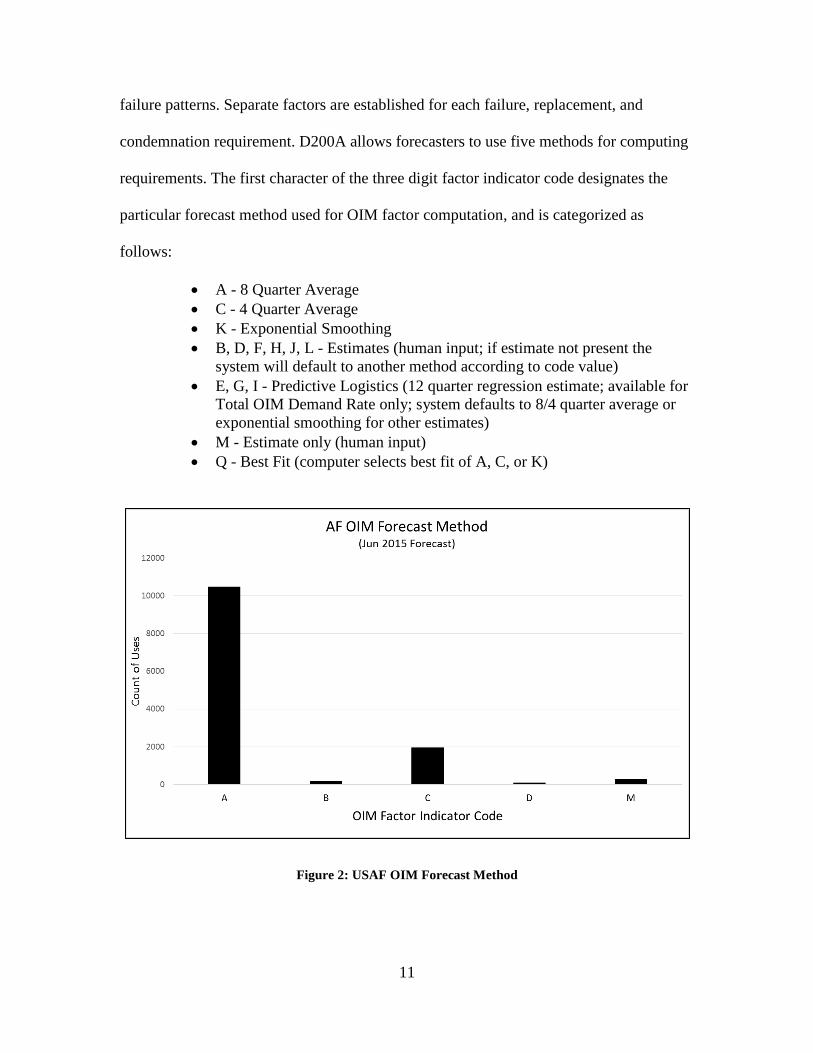
failure patterns. Separate factors are established for each failure, replacement, and
condemnation requirement. D200A allows forecasters to use five methods for computing
requirements. The first character of the three digit factor indicator code designates the
particular forecast method used for OIM factor computation, and is categorized as
follows:
A - 8 Quarter Average
C - 4 Quarter Average
K - Exponential Smoothing
B, D, F, H, J, L - Estimates (human input; if estimate not present the
system will default to another method according to code value)
E, G, I - Predictive Logistics (12 quarter regression estimate; available for
Total OIM Demand Rate only; system defaults to 8/4 quarter average or
exponential smoothing for other estimates)
M - Estimate only (human input)
Q - Best Fit (computer selects best fit of A, C, or K)
Figure 2: USAF OIM Forecast Method

12
Looking at Figure 2, it is easy to see that the USAF primarily uses an eight
quarter and a four quarter moving average that is proportional to the number of flying
hours flown. These are nearly 80% and 15% respectively, of the total base-level forecast
methods used. There are many instances where this method, often called the proportional
model, works very well. The main explanation is because of the fact that the calculation
incorporates a robust amount of data. To elaborate, consider a lumpy demand cycle. The
eight quarter average has the ability to slowly trend upwards or downwards depending on
the tendency. As each data point is weighted equally, no one point is overly influential,
making the computation more resilient to sporadic change. Additionally, several studies
agree that as long as the aircraft continues to fly relatively similar operations, the
proportional flying hour method with an eight quarter moving average are typically
adequate forecasting methods (Slay & Sherbrooke, 1998; Wallace et al., 2000).
USAF Forecast Accuracy
There is a long history of U.S. Government Accountability Office (GAO)
investigations into DoD spare parts practices. The first was in a 1984 report, when the
GAO estimated that the USAF overstated $31.1 million in needs for aircraft being phased
down or phased out, while simultaneously under estimating $28.8 million need for new
aircraft needs (U.S. General Accounting Office, 1984). Furthermore, the GAO felt the
issues were a result of miscalculations driven from the very same flying hour
proportional model used today. After an estimated $30 billion in excess parts was
discovered, inventory management was consequently added to the High Risk List (U.S.
General Accounting Office, 1990). In 2013, another GAO study was completed and
estimated spare parts excess inventories at $9.2 billion (U.S. Government Accountability

13
Office, 2013). While marginal steps were taken to eliminate waste, there was still more
work to be done. The 2013 report stated that with regard to inventory management, there
were nine key areas needing improvement, one of which was demand forecasting. It was
specifically noted that the DoD was in the early stages of implementing numerous actions
to improve demand forecasting. Finally, as recently as 2015, inventory management was
cited again as still lacking “demonstrated progress” in order to be removed from the GAO
High Risk List (U.S. Government Accountability Office, 2015).
Lowas, an independent researcher, performed a very rigorous analysis of the
USAF’s forecasting methods. First, to get an overall sense of accuracy, he utilized the
USAF’s web based Forecast Analysis Comparison Tool Plus (FACT+). He limited his
analysis to airframe (structural) components, noting that previous studies showed this
category of parts to have the highest forecast accuracy. Here he found that the aggregate
forecast accuracy for airframe NIINs was approximately 50% over the 2010-2011 period
(Lowas III, 2015). He then further refined his purview by filtering out NIINs with
intermittent and sporadic demand, as well as NIINs with small sample sizes. This left him
only with items that displayed smooth demand. Table 1 shows the forecast accuracy of
the most common forecasting methods used by the USAF (excluding Hotl’s). Even with
isolating what should be definitively the most predictable parts, the USAF’s best result is
narrowly better than a 30% forecast error with an eight quarter moving average.
Additionally, when analyzing lumpy demand patterns, errors rose well over 40%. Lowas’
final judgment was that “it is apparent that current common forecasting methods are
inadequate for aircraft spare parts forecasting” (Lowas III, 2015).

14
Table 1: Smooth Structural NIINs and Associated Forecasting Accuracies (Lowas III, 2015)
Demand Forecast Accuracy
There are multiple ways to measure forecast error or accuracy. Demand Forecast
Accuracy, the method the USAF uses, is calculated as (FACT+ User Manual, 2016):
𝐷𝐹𝐴 = 1 −∑ |𝐴𝑐𝑡𝑢𝑎𝑙 𝐷𝑒𝑚𝑎𝑛𝑑−𝐹𝑜𝑟𝑒𝑐𝑎𝑠𝑡 𝐷𝑒𝑚𝑎𝑛𝑑|𝑛𝑖=1
∑ 𝐴𝑐𝑡𝑢𝑎𝑙 𝐷𝑒𝑚𝑎𝑛𝑑𝑛𝑖=1
(1)
where n is the number of periods aggregated in the forecast horizon. Note that this
calculation is really a calculation of one minus the forecast error, which results in an
accuracy measurement. In instances where actual demand is zero, to avoid an undefined
result the FACT+ tool defines these results as -999% or non-applicable (FACT+ User
Manual, 2016). This practice has large issues, particularly on parts with intermittent or
lumpy demand patters which frequently have periods with no demand.
A more commonly accepted forecast error measurement is mean absolute percent
error. This calculation has the benefit of being scale independent, and therefore can
compare error across multiple series of forecasts (Hyndman, 2006). The main difference

15
between demand forecast accuracy and mean absolute percent error is that the latter
divides both the numerator and denominator by n, and leaves the expression in terms of
error, instead of subtracting from one.
Hyndman (2006) shows how mean absolute percent error, and subsequently
demand forecast accuracy, frequently result in biased distributions when actual demand is
close to zero. Again, actual demand values that are close to zero are common for
intermittent and lumpy demand items. Additionally, this calculation puts a heavier
penalty on positive errors than on negative errors, which adds to the biased result
(Hyndman, 2006). Because of this, analysts should be strongly cautioned from using
these measurements as valid forecast error tools in which accuracy measurements will be
evaluated on. In light of this knowledge, Hyndman (2006) recommends a new calculation
called mean absolute scaled error. This calculation has been shown to be non-biased and
more applicable for intermittent demand patterns. For these reasons, mean absolute
scaled error will be the error measurement used in this study. A detailed description of
this calculation is denoted in the Chapter III.
Replacement Parts Forecasting
This next section will discuss common parts forecasting methods used in spare
parts forecasting. Tibben-lembke and Amato (2001) reference a number of surveys that
have shown that the most common replacement parts forecasting methods are weighted
moving averages, straight-line projections, and exponential smoothing. This corroborates
common understanding that simpler methods are often implemented because of ease of
use. A hierarchy diagram lists the most common forecast methods in Figure 3.

16
Figure 3: Hierarchy of Forecasting Methods (Lowas III, 2015)
Tibben-lembke and Amato go on to elaborate on the value information can add to
forecasting methods. They estimate failure using an exponential distribution. The benefit
of the exponential distribution over the Weibull is that it only has one distribution
parameter that can be estimated easily as mean time between failures. Their analysis
showed this method to be more precise than exponential smoothing and weighted moving
average (Tibben-lembke & Amato, 2001). A connection here should be made to a similar
premise to this thesis research, in that additional information is being used to form a new
forecast method with explanatory variables in lieu of a purely historic forecasting
technique.
In reliability theory, the Weibull distribution is commonly used to model the
failure of spare parts (Lowas & Ciarallo, 2016). Lumpy or sporadic demand are very
common issues among aircraft parts forecasting, making it very difficult to be accurate.
However, the root cause of this pattern had never fully been vetted (Lowas & Ciarallo,

17
2016). Boylan (2005) provided a rule of thumb for sporadic demand parts as having at
least 20% of time periods with zero demand. Lowas and Ciarallo (2016) explored the use
of the Weibull distribution in order to find fleet-wide variables that may cause lumpy
demand patterns. They used a Monte Carlo simulation to measure fleet-wide demand
characteristics by comparing ranges of fleet sizes, buy period lengths, time to failure
lengths, as well as varying Weibull distribution parameters. Results of the Monte Carlo
simulation show that the variable that increased lumpy demand the most was aircraft fleet
size. The second largest variable accounting for lumpiness was the buy period. The
observation was that a longer buy period increased demand variability (Lowas &
Ciarallo, 2016).
Several other researchers have addressed the issue of sporadic demand for the
USAF. In 2007, Bachman formulated a Peak inventory policy that reduced wholesale
wait-time and backorders by establishing a new reorder point based on exponential
smoothing of an item’s peak demand pattern. In 2013, he established a new inventory
policy that assessed item cost, procurement and repair lead times, and overall demand
patterns to build a cost versus aircraft availability tradeoff curve (Bachman, 2013). This
method is used today throughout the USAF, and is known as Readiness Based Sparing.
Gehret (2015) looked at a stockage policy based on how likely a specific location is to
have a demand, given the population’s demand and that location’s time since its last
demand. The takeaway from the above three studies is that in lieu of a strong demand
signal, inventory policies are the method used to provide a high level of supportability in-
place of demand forecasting techniques. The benefit of CBM is that it does not rely solely

18
on a demand signal. Instead, it offers the ability to use conditional data as will be
discussed later in this chapter.
Alternative USAF Forecasting Models
Work done by Oliver (2001) used linear regression to correlate F-16 mission
capability rates with numerous explanatory variables. Oliver’s work had a very broad
aperture of variables considered. A few examples were maintenance manning,
maintenance skill levels, maintenance retention, aircraft break rates, aircraft fix rates,
flying operations tempos, and spare parts issues among many other variables including
spare parts funding. His results showed that a predictive mission capability model
included the number of sorties, flying hours, average aircraft inventory, total maintenance
personnel assigned, and controlling for interactions between total maintenance personnel
and average aircraft inventory. The significance of this research pinpointed controllable
inputs that decision makers could use to improve MC rates. In 2013, Theiss performed a
similar investigation by evaluating which variables would characterize C-17 mission
reliability. His analysis concluded that mission type, operating organization type,
departure theater, aircraft age, as well as other variables are significant. Such research
like these will serve as fodder for explanatory variables used in this research. Even
though not all of these variables will be used in this work, the premise of using event data
to explain parts failure is of a similar line of reasoning.
To this point, the appropriateness of the proportional flying hour failure model
has only been subtlety questioned. However, there are several studies which directly
uncover the fallacies with its use. Before looking at other research efforts, let us first

19
discuss what a similar proportional cost model assumes. Van Dyk (2008) defines the
model as a proportional relationship between costs and flying hours such that:
1. When no hours are flown costs are zero.
2. A 1% increase in flying hours will increase costs by 1%.
The spare parts proportional model definition is presumably the same for demand
forecasting; as total costs are merely a function of the number of parts demanded.
One organization who has performed several research efforts on the proportional
model is the Logistics Management Institute (LMI). A 1995 study performed by LMI on
war time demands showed that a pure flying hour approach would overstate demands,
while a pure sortie-based approach would understate demands as shown in Figure 4
(Slay, 1995).
Figure 4: Proportional Flying Hour Model Vs. Sortie Model (Slay, 1995)
A more rigorous study was then completed by LMI two years later showing that after
analyzing 250,000 sorties, a 2-hour fighter sortie caused only 10% more parts to break
than a 1-hour sortie did (Slay & Sherbrooke, 1998). This refutes the second principle of
20
Van Dyke’s (2008) definition because a 2-hour sortie should have produced a 100%
increase in broken parts over a 1-hour sortie under the proportional model. This concept
led the analysts to look at the problem through another lens; one that shifted toward
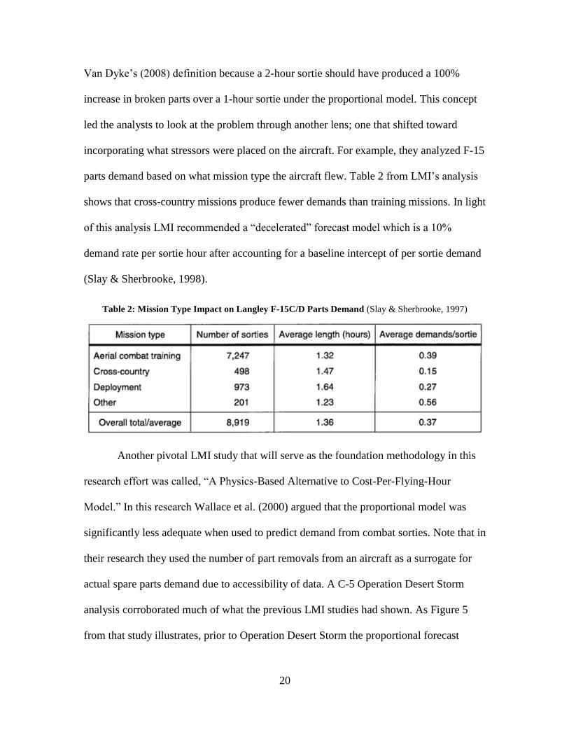
incorporating what stressors were placed on the aircraft. For example, they analyzed F-15
parts demand based on what mission type the aircraft flew. Table 2 from LMI’s analysis
shows that cross-country missions produce fewer demands than training missions. In light
of this analysis LMI recommended a “decelerated” forecast model which is a 10%
demand rate per sortie hour after accounting for a baseline intercept of per sortie demand
(Slay & Sherbrooke, 1998).
Table 2: Mission Type Impact on Langley F-15C/D Parts Demand (Slay & Sherbrooke, 1997)
Another pivotal LMI study that will serve as the foundation methodology in this
research effort was called, “A Physics-Based Alternative to Cost-Per-Flying-Hour
Model.” In this research Wallace et al. (2000) argued that the proportional model was
significantly less adequate when used to predict demand from combat sorties. Note that in
their research they used the number of part removals from an aircraft as a surrogate for
actual spare parts demand due to accessibility of data. A C-5 Operation Desert Storm
analysis corroborated much of what the previous LMI studies had shown. As Figure 5
from that study illustrates, prior to Operation Desert Storm the proportional forecast

21
model worked adequately. Under the proportional model, when flying operations
increased under Operation Desert Storm, then removals should subsequently increase as
well. However, the actual number of removals stayed relatively the same regardless of
the increase in flying hours per month.
Figure 5: Operation Desert Storm C-5 Analysis (Wallace et al., 2000)
On the back of this research and previous studies, this LMI team decided to
segregate forecast parameters based on combat sorties and training sorties. From this they
established the Physics-Based Model (PBM), which incorporates predictor variables that
were driven by the physical behavior of the aircraft such as the number of landings, the
number of sorties, and the number of hours on the ground in addition to flying hours
(Wallace et al., 2000). In order to test their model’s accuracy relative to the proportional
model, they compared four separate time series data sets for the C-5, the C-17, the KC-

22
135, and the F-16. The PBM had a lower forecast error in each of the 16 cases analyzed
(Wallace et al., 2000).
CBM Philosophy
A simple description of a Condition Based Maintenance (CBM) system was
postulated by Jardine, et al. (2006), stating that every CBM system has three steps. First,
is data acquisition. This step is centered on obtaining data on the health of the system.
Second, is data processing; which is analyzing the signals from step one. The final step is
maintenance decision-making, which revolves around making policies that drive
maintenance actions based on the analysis from step two.
CBM is a maintenance strategy that bases decisions on information collected
through condition monitoring (Ellis, 2008). Prajapati, Bechtel, and Ganesan (2012)
postulate that CBM is a subset of reliability centered maintenance, which is made up of a
mix between CBM and scheduled (preventative) maintenance. The primary goal of CBM
aims at avoiding unnecessary maintenance tasks until there is significant evidence of
need (Jardine et al., 2006). Maintenance actions based on this premise can lead to
remaining useful life improvements, resulting in lower maintenance costs (Tracht, Goch,
Schuh, Sorg, & Westerkamp, 2013). This notion contrasts that of scheduled maintenance
which relies on fixing or replacing a part based on a designated time (or use) interval
regardless of the actual condition of the part.
Diagnostics/Prognostics
Diagnostics is defined as the process of finding a fault after or during the process
of the fault occurring in the system (Prajapati et al., 2012). This analysis is performing

23
fault detection, isolation or identification with posterior event data (Jardine et al., 2006).
The following section will elaborate on the aspects of this type of analysis. Prognostics in
the realm of machine data analysis is defined as the process of predicting the future
failure of any system, by analyzing current and previous history of operating conditions
(Prajapati et al., 2012). This application is different from diagnostic in that it explicitly
performs prior event analysis so it can predict or forecast a failure event (Jardine et al.,
2006).
Event Data
Event data are descriptors of the physical history of a particular machine.
Examples could include installation, breakdown, overhaul, preventative maintenance
action, oil change, number of uses, etc. (Jardine et al., 2006). These data are typically
entered into a database by hand, making them prone to errors.
Condition Monitoring Data
Condition monitoring data are typically collected through sensors. Depending on
equipment being monitored, the sensors may be measuring vibrations, acoustics, oil
analysis results, temperature, pressure, moisture, humidity, weather or environmental
factors, etc. (Jardine et al., 2006). These types of data, sometimes called covariates, can
identify deterioration, resulting in time to failure (TTF) models. Common descriptive
data analysis tools such as clustering or multivariate analysis can be used to assess which
variables will be useful to detect part failures. Murray, et al. compare multiple fault
detection algorithms including support vector machines, rank-sum, and recommend their
own naïve Bayesian classifier called the multiple-instance naïve Bayes (mi-NB)
algorithm. Their study specifically assessed the varying method’s ability to detect fault
24
from a multiple-instance learning environment (many simultaneous condition indicators).
This is useful in cases involving multiple sensors on one part; each with their own limits
set to trigger a fault indicator (Murray, Hughes, & Kreutz-Delgado, 2005). Results of
their study show that support vector machines achieved the highest accuracy, however
computationally took longer than other methods. Their proposed method, mi-NB, serves
as a good model that balances both accuracy and speed (Murray et al., 2005).
CBM+ in DoD
As mentioned earlier, CBM first came into the DoD’s lexicon in 2002. The DoD
established the term Condition Based Maintenance Plus (CBM+), which refers to
integrating technologies for the purpose of enhanced prognostic capabilities. The USAF’s
journey establishing a CBM+ program began in 2003, where the Air Force Logistics
Management Agency completed a concept analysis, and provided recommendations for
implementing CBM+ (T. Smith, 2003). In 2007, the USAF had a central office
orchestrating the future state picture of reliability prognostics that lasted for nearly a
decade. This organization was charged with orchestrating a common system
infrastructure and accompanying services for integrating all combat support IT systems
(Navarra et al., 2007). More specifically, they set their sights on improving maintenance
agility and responsiveness in order to increase operational availability, and to reduce
lifecycle total ownership costs.
In order to assemble this IT infrastructure, the USAF contracted with a database
management company named Teradata who built a proprietary high-performance
distributed computing architecture, complete with data bus that enables integrated

25
throughput between multiple computing nodes (Navarra et al., 2007). The result is now
referred to as the Logistics, Installation, and Mission Support–Enterprise View (LIMS-
EV), and is made up for multiple suites to access data universes. The backbone of this
system is the Global Combat Support System-Data Services which stands as the central
data warehouse for most of the USAF’s logistics IT systems. In addition to the IT
infrastructure, the USAF’s CBM+ office established the Enterprise Predictive Analysis
Environment. The thought was that this node would act as a central hub for building
prognostic algorithms that could leverage data sets across all logistics IT systems from
the LIMS-EV package. Figure 1 (in chapter 1) shows a system diagram of how the
Global Combat Support System-Data Services and the Enterprise Predictive Analysis
Environment components fit into the CBM+ proposed model. There were three
capabilities the USAF wanted to obtain from this structure (Navarra et al., 2007):
To predict any weapon system’s mission capability
To proactively maintain readiness
To design for integrated system life cycle management and intrinsic
reliability
Many organizations have identified difficulties implementing CBM programs
(Jardine et al., 2006). Similarly, the USAF struggled with implementing these practices as
well. According to Navarra et al. (2007), the premise was to have operational data
captured during flight and post-flight inspections automatically downloaded into LIMS-
EV. Raw data would come from sensors on the aircraft or from maintainers on the flight
line. These data, along with event data, could be analyzed by the Enterprise Predictive
Analysis Environment, whom would build predictive algorithms resulting in a remaining
useful life estimate for major components on the airframe. However, the major problem

26
was integrating pedigree data directly from sensors into the Global Combat Support
System-Data Services data warehouse (Navarra et al., 2007). As such, analysts were
forced to resort to using small samples for statistical estimates or simulation data for
prognostics.
Previous USAF researchers have also identified issues with regard to reliability
failure data in USAF systems. Hogge (2012) attempted to calculate failure distributions
of USAF end items, yet stated in his research that the only time to failure data the USAF
collected was mean time between failures. He goes on to discuss the issue with mean
time between failure being that this calculation is both left and right censored.
Furthermore, the mean time between failure calculation is not a depiction of a part’s
entire useful life. Without that information, a reliability distribution cannot be computed.
Further, he illustrates that the USAF tracks usage hours for equipment, usually aircraft or
engines, however there is no usage tracking mechanism for most subsystems.
Current CBM+ USAF guidance is extremely sparse. The central document
describing today’s CBM+ efforts is a two page fact sheet which provides a general
description of CBM and CBM+. It states that CBM+ is a meaningful shift away from a
reactive, unscheduled maintenance approach to an evidence of need before failures
approach (U.S. Air Force, n.d.). Additionally, the fact sheet provides a few examples of
how CBM+ can and is used throughout the USAF. Of note, the source alludes to the
USAF currently using sensors that monitor and record equipment operating parameters to
facilitate remote analysis. Specifically the sheet references the CBM+ application to the
F-35 because of its unique Automated Logistics Information System. However, even as
recent as 2016, this automated logistics system is not yet fully operational (GAO, 2016).

27
Therefore, this system was not currently a viable resource option for collecting data.
Subsequently, it became a priority to identify where other similar CBM+ analysis was
occurring throughout the USAF. A 2014 study on the impacts of CBM in the military was
completed by the Australian military. This land centric analysis showed that there are
three main impacts (Gallash, Ivanova, Rajesh, & Manning, 2014):
CBM will extend equipment’s useful life while reducing the total cost
CBM will increase fleet operational availability and mission effectiveness
CBM will reduce the maintenance burden
It is reasonable to extrapolate these same benefits within an aviation context. Ellis (2008)
believed that CBM should only be applied where condition monitoring techniques are
available in a cost-effective means. Prajapati et al. (2012) asserted aviation as being a
cost-effective CBM area both because of the value the aviation community places on
safety, the capital intensiveness of aircraft, and the value to be gained from extending the
life of the system. The USAF followed that business model by stipulating that the F-35
have condition monitoring capability from the beginning of its design, therefore making
it more cost effective than adding sensors later (U.S. Air Force, n.d.). Further, Swanson
(2001) corroborates the benefit to fleet operational availability, as equipment would then
only taken out of service when direct evidence necessitates maintenance.
Evidence of what Gallash, et al. (2014) postulated was exemplified all the way
back in a 1980s U.S. Coast Guard contract, specifying engine condition monitoring
requirements for the HH-65A. This contract delineated each of the condition monitoring
sensors already on the helicopter’s engine that could be used for analysis, and spelled out
the type of data analysis they were going to be able to use based on the condition
monitoring signals (Aerospatiale Helicopter Corporation, 1980). At that time engine
28
sensors would allow experts to perform CBM analysis on engine torque, gearbox
temperature, oil pressure, oil filter impending bypass quantity, gas temperature, and
generator speed.
The Army also recognized the need to move away from a scheduled maintenance,
but knew it did not have the IT system in-place to do so. An effort was made in 2005 to
canonize the IT requirements that would allow Army analysts to perform CBM
diagnostics and prognostics (Figure 6). First, they identified the fundamental data
needs—a comprehensive and synchronized view of a component’s lifecycle (Henderson
& Kwinn, 2005). From this, their analysts could aggregate trends of problem occurrences
within major systems. Then these trends could be juxtaposed to an individual
component’s life history where reliability forecasts could be stipulated based on a
component’s current condition. One of the major issues their report noted was a disparity
between maintenance and supply codes. Specifically they recognized the importance of
having a link between work unit code (which is primarily used in the maintenance
community) and national stock numbers (used by the supply community) (Henderson &
Kwinn, 2005). Without this link, analysts would lack the ability to pinpoint which aircraft
system a specific component belongs to, thereby limiting the ability to drill down to
analyze multiple layers of a weapon system. Further, another critical shortcoming the
Army’s legacy systems lacked was a unique part identification. They describe this as a
requisite capability in order to track a specific item through its lifecycle. Without a
unique identification, they stipulate that “CBM implementation will be limited”
(Henderson & Kwinn, 2005).

29
Figure 6: Affinity Diagram of CBM Data Warehouse Components (Henderson & Kwinn, 2005)
The U.S. Navy’s pursuit of a CBM strategy led them to use the Integrated
Mechanical Diagnostic-Health Usage Management System (IMD-HUMS). This system
enabled Reeder to perform CBM analysis on phase inspection maintenance on the MH-
60S helicopter. The background of his study was similar to this thesis, in that the U.S.
Navy had been working to implement CBM methods for over two decades, however still
primarily relied upon inspection cycles (Reeder, 2014). This notion led him to study the
effects of an evidence based inspection cycle relative to the baseline phase inspection
cycle by comparing data already collected in IMD-HUMS. A gap analysis between the

30
baseline and the CBM alternative method led to the conclusion that the alternative was
superior in multiple areas. The first area assessed showed that the added flight hours
available per labor hour during phase inspections rose from 0.35 flight hours per phase
labor hour, to 1.07 flight hours per phase labor hour (Reeder, 2014). The second area
showed a reduction in post-phase vibration analysis thru evidence based inspections of
engine and drive train systems. Results showed available flight hours increased by 3.24%
(Reeder, 2014). The availability gain came from eliminating post-phase scheduled
inspections. Further, maintenance labor hours decreased by an average 1,270 hours per
phase cycle. Lastly, there might be a hesitance to move away from what had been the
status-quo schedule inspection cycle, so Reeder included a safety analysis. His
investigation showed that 60% of all mechanical failures from the preceding five years
came from human error. Therefore, by reducing the number of human occurrences to
perform maintenance, you reduce the amount of potential human error. He concluded that
there was no evidence to show that his alternative need-based phase model would
compromise safety in a meaningful way.
CBM Forecast Methods
A time-dependent proportional hazards model (PHM) is a common method used
in survival analysis, and can be used to assess both event data and condition monitoring
data together (Jardine et al., 2006). The PHM is calculated as:
ℎ(𝑡) = ℎ0(𝑡)exp (𝛾1𝑥1(𝑡) + ⋯+ 𝛾𝑝𝑥𝑝(𝑡)) (2)
where ℎ0(𝑡) is a baseline hazard function, 𝑥1(𝑡), … , 𝑥𝑝(𝑡) are covariates from condition
variables, that are a function of time, and 𝛾1, … , 𝛾𝑝 are coefficients. Then, a maximum

31
likelihood estimator method can be used to find the 𝛾𝑖 coefficients for the PHM from
event data and condition monitoring data (Jardine, Anderson, & Mann, 1987). The
necessary inputs for this method are a hazard function, and condition indicator covariates.
The PHM produces a hazard distribution that is descriptive of the item being assessed.
Another common method that uses both event data and condition monitoring data
is a hidden Markov model (HMM). A significant contribution was made by Wang in
developing a model for combining both continuous and categorical state descriptors into
one HMM. His model is based on a two-stage approach separating a component’s life
into a normal working zone and a potential failure zone (Wang, 2007). Further, he shows
analytically how continuous and categorical descriptors can be combined in a maximum
likelihood estimator to model which state a component is in, and the probabilistic time to
failure (Wang, 2007). This research is influential because of its ability to model the TTF
distribution from practical state descriptors.
Moubray (1997) formed a method known as the P-F interval method, which uses
condition monitoring data to predict the failure probability of a component. In this
method, a P-F interval is the time between a potential failure (P) and a functional failure
(F). This method was enhanced by Goode et al. by combining reliability data with
condition monitoring data, to predict the time to failure of steel mill plant machinery
(Goode, Moore, & Roylance, 2000). They did this by separating condition monitoring
observations into two regions a stable zone and a failure zone, where two distinct failure
distributions can be observed. Based upon these observations, a component’s remaining
useful life can be predicted by a reliability-based model for parts in the stable zone, a

32
combination of a condition monitoring indicator, and a reliability model for components
in the failure zone (Goode et al., 2000).
Several researchers have established a Bayesian approach that can be updated by
conditional monitoring information. Gebraeel, et al. laid the foundation for this area of
study with a technique called the Bayesian Degradation Signal Model. Their approach
had two key elements. The first was to use population parameters to form a prior failure
distribution. This would predict when and how many bearings would fail. The second
element was real-time condition monitoring data, which showed the degradation of an
individual bearing (Gebraeel, Lawley, Li, & Ryan, 2005). Their research demonstrated
that if the population’s failure was properly modeled, real-time condition monitoring
could then be used to compute a residual-life distribution for that particular bearing.
Tracht, et al., (3013) were able to formulate a forecasting approach using a
supervisory control and data acquisition (SCADA) program that predicted spare parts
demand. Their method, noted as an “enhanced forecast model,” was a PHM capable of
incorporating time dependent covariates, as well as temperature and age conditions. The
significance of this work was showing how SCADA software could be used to formulate
an accurate binomial PHM distribution.
Kalman filters can also be applied to condition based prognostic models. One
example was demonstrated by Swanson, who used Kalman filtering to track the changes
in condition monitoring data across a time horizon (D. Swanson, 2001). With this,
Swanson was able to both detect fault and make useful life predictions. He postulates that
when fault characteristics are accelerating away from a stable operating condition, there
is a probable chance of imminent failure which can serve as an indicator (D. Swanson,
33
2001). Furthermore, tracking the rate of change of a part’s condition allows the ability to
make a prediction.
A summary the CBM forecasting methods can be found in Appendix B:
Diagnostic and Prognostic CBM Summary.
Summary
This chapter examined spare parts forecasting both in the USAF and at large.
Several alternative USAF demand forecasting methods were presented that illustrate how
alternative variables than flying hours can be predictive of parts demand. Further, a
history of CBM+ in the DoD was discussed to illustrate what the original goal was, and
where the program is currently. An academic view of CBM prognostic techniques was
discussed to show what types of data and analyses the DoD could implement when the
proper data is available. Lastly, several forecast error calculations were presented to
explain why mean absolute scaled error is more suitable for spare parts forecasting.

34
III. Methodology
Chapter Overview
This chapter will explain how the PBM works, and how it will be applied in this
research. It will start by identifying the explanatory variables and the model’s
assumptions. Then, the statistical background of how to calibrate the model’s parameters
will be explained. Following this, a detailed effort will be made to delineate the data
cleaning and filtering steps taken to narrow down to a select list of NIINs used in this
study. Finally, calculations for forecast accuracy will be presented along with a
discussion on multivariate statistics that will be applied to evaluate the suitability of one
forecast method over another.
PBM Basics
A majority of the methodology used in this research effort was leveraged from a
research effort completed by Wallace and Lee (2000), which first tried to consider how
physical stressors on an aircraft reflect in maintenance removal actions. The approach
taken in this research will apply a similar tactic looking at NIIN level demand patterns.
LMI’s model originally included four independent variables:
Flying Hours (FH)
The LMI model treated flying hour-induced removals as a discrete Poisson
distribution, where the number of flight-induced removals produced in time 𝑡𝑓 has
parameter 𝜆𝑓𝑡𝑓 . A normal approximation to the Poisson distribution can then be used to
35
calculate the number of removals with mean and variance of fling-hour-induced removals
both equal to 𝜆𝑓𝑡𝑓 (Wallace et al., 2000).
Cold Cycles (CC)
A cold cycle was the approach taken to account for removals induced from a
sortie. The term cycle is used to frame the effects of both the take-off and the landing
inherent to each sortie, regardless of what is done during the course of that sortie. The
number of cold cycles will equal the number of sorties in a given time period. This aspect
was modeled as a normal approximation to a binomial distribution where 𝑁𝑐𝑐is the
number of cold cycles and 𝑃𝑐𝑐 is the probability of a removal per cold cycle. This means
that this process can be modeled with mean 𝑁𝑐𝑐𝑃𝑐𝑐 , and variance 𝑁𝑐𝑐𝑃𝑐𝑐(1 − 𝑃𝑐𝑐)
(Wallace et al., 2000).
Warm Cycles (WC)
It could be assumed that the effects of a touch and go landing are different than
the stress from a cold cycle, which includes starting up the jet and shutting it down with
each sortie. Therefore, this variable will equal the number of landings minus the number
of sorties in a given time period. This aspect will also be modeled as a normal
approximation to a binomial distribution where 𝑁𝑤𝑐is the number of warm cycles and 𝑃𝑤𝑐
is the probability of a removal per warm cycle. This process is therefore modeled with
mean 𝑁𝑤𝑐𝑃𝑤𝑐 , and variance 𝑁𝑤𝑐𝑃𝑤𝑐(1 − 𝑃𝑤𝑐) (Wallace et al., 2000).
Ground Cycles (GC)
This aspect of the LMI model describes strain on an aircraft that would come
from the ground environment, mostly being environmental influences such as
temperature, humidity, or precipitation. This variable is computed as possessed hours

36
minus flying hours in a given time period, divided by 24 hours to convert hours into a
daily cycle. Similarly to cold and warm cycles, ground cycles are also modeled as a
normal approximation to a binomial distribution. Mean and variance are then calculated
as 𝑁𝑔𝑐𝑃𝑔𝑐 and 𝑁𝑔𝑐𝑃𝑔𝑐(1 − 𝑃𝑔𝑐) , respectively (Wallace et al., 2000).
Model Mean and Variance
The methodology taken in this effort utilizes the same four independent variables,
however assess the effects on a different dependent variable, aircraft parts demand.
Therefore, the same variable computations will be used and aggregated as:
𝜇𝑖 = 𝜆𝑓𝑡𝑓 + 𝑁𝑐𝑐𝑃𝑐𝑐 + 𝑁𝑤𝑐𝑃𝑤𝑐 + 𝑁𝑔𝑐𝑃𝑔𝑐 (3)
𝜎𝑖2 = 𝜆𝑓𝑡𝑓 + 𝑁𝑐𝑐𝑃𝑐𝑐(1 − 𝑃𝑐𝑐) + 𝑁𝑤𝑐𝑃𝑤𝑐(1 − 𝑃𝑤𝑐) + 𝑁𝑔𝑐𝑃𝑔𝑐(1 − 𝑃𝑔𝑐) (4)
where 𝑖 is the index indicating each time period (Wallace et al., 2000).
Model Assumptions
The PBM has two main assumptions. The first assumption is that the four
explanatory variables are independent from one another. If any two independent variables
are collinear, then one should be removed as to not over influence the model. This will be
evaluated by a pairwise regression to tell if each pair of variables has a strong correlation.
The second assumption is that spare parts failure can be attributed to the four
independent variables in high enough quantities to be approximated as a normal
distribution. This assumption reduces the computational complexity behind estimating
the number of failures in a time period. Wallace and Lee (2000) use this assumption in
their research, and results were found to be very accurate.

37
=∏𝑓(𝑥𝑖|𝜃)
𝑛
𝑖=1
𝑙 =∑ln [𝑓(
𝑛
𝑖=1
𝑥𝑖|𝜃)]
Model Calibration: Maximum Likelihood Estimation
In order to use the PBM forecast, the parameters from the four independent
variables must be fine-tuned to the appropriate failure probability. Due to
homoscedasticity in demand, a simpler method such as linear regression is not possible.
Therefore, a maximum likelihood estimation will be used to calibrate the respective
probability parameters. Maximum likelihood estimation is a well-established method that
uses conditional probability to determine a distribution’s parameter value, given that a set
of data came from that particular distribution. For example, consider the likelihood
equation:
𝐿(𝜃) = 𝑓(𝑥1, 𝑥2, 𝑥3…𝑥𝑛; 𝜃) (5)
This is the joint probability of a distinct set of outcomes 𝑥1, 𝑥2, 𝑥3…𝑥𝑛 . From the rules
of conditional probability given that each outcome is independent, the likelihood
probability of outcomes becomes:
𝐿(𝜃|𝑥𝑖) = 𝑓(𝑥1|𝜃) ∙ 𝑓(𝑥2|𝜃) ∙ 𝑓(𝑥3|𝜃) ∙ … ∙ 𝑓(𝑥𝑛|𝜃)
(6)
Then by taking the natural logarithm of the equation, the function becomes additive,
which is much easier for computational purposes as shown in Equation 7:
(7)
If solving this problem numerically, the next step would be to find where this function is
maximized by finding its derivative with respect to 𝜃, and then setting it equal to zero.
The value where the maximum likelihood occurs will be the optimal value of 𝜃 for the
38
given dataset. However, this operation is easily performed in Microsoft Excel (version
2013) by using the Solver function to solve this as an optimization problem. In this
instance, because there are four parameters to be calibrated, the optimization problem
becomes:
𝑀𝑎𝑥:∑ ln [𝑁(𝑑𝑒𝑚𝑎𝑛𝑑𝑖|𝜇𝑖, 𝜎𝑖)]𝑛𝑖=1 (8)
where n is the number of periods in the calibration horizon, and 𝑁(𝑑𝑒𝑚𝑎𝑛𝑑𝑖|𝜇𝑖, 𝜎𝑖)
assumes a normal approximation with parameters and i from Equation 3 and Equation
4. The change variables will be 𝜆𝑓 , 𝑃𝑐𝑐 , 𝑃𝑤𝑐, 𝑃𝑔𝑐 .
Sliding Scale
The concept of a sliding scale was not in LMI’s original PBM study. However, it
was developed out of necessity to be able to forecast into the future when a different
flying profile would be used. To elaborate, consider the original premise behind the PBM
model. It was to show that parts failure is driven by what physical stresses are induced on
the aircraft. Their research uncovered how a large increase in combat flying hours did not
keep the proportional relationship with demand. From this, they postulated that the
effects on parts failure are noticeably different on training missions than on combat
missions. Their later research used an approach that allowed an analyst to forecast a
future periods’ demand, by choosing a new proportion of combat missions to training
missions (Silver & Cincotta, 2008). The basic premise is that the model uses the actual
flying profile to determine the average sortie duration for peacetime missions and combat
missions separately. Similarly, it also calculates the average landing per sortie for
peacetime missions and combat missions, respectively.

39
A major assumption in this research will rely on using the actual flying profile in
a forecasted period as if it were as forecast parameter. In a real application of the PBM
method, the flying profile would be another forecast parameter similar to total flying
hours. However, in order to isolate this model’s forecast potential, it will be assumed that
the forecasted flying profile was what was actually flown for each time period predicted
into the future.
Next, the respective average sortie duration and landings per sortie values could
be used to linearly extrapolate a future time period’s number of sorties and number of
touch-and-go landings, again broken out for peacetime and wartime. Subsequently, there
needs to be a similar methodology of calculating ground cycles. Since the original model
does not assume a difference between ground cycles in training versus in combat, this
single parameter only needs to be adjusted for the forecast period’s number of flying
hours. This can easily be done by assuming the number of unit possessed hours as the
prior period which was known, subtracting the forecast period’s number of flying hours,
and then dividing by 24. The next step would be to sum the total number of sorties and
“touch-and-go’s” that could then be used as forecast inputs against the failure rate
parameters calibrated by the maximum likelihood estimator. A list of equations used in
this process is delineated in Appendix C: Sliding Scale Equations.
Data
Sources
Two primary data sources would be used to collect data, with the first being the
parts failure data maintained in D200A. With the help of the Requirements Integration

40
Process Improvement Team, AFSC/LGPS, a filter of B-1 only NIINs was used to select
quarterly OIM data for B-1 NIINs. Using Microsoft Access (version 2013), a query was
then built to aggregate base-level demand, and to select file maintained data (manual
override corrections) when applicable over original data inputs. Base-level demand (more
accurately defined as Total OIM Demand) is computed as the number of parts Repaired
This Station (RTS) plus the number of parts Not Repaired This Station (NRTS) plus the
number of Condemnations as shown in Equation 9: (Air Force Materiel Command, 2011)
𝑇𝑜𝑡𝑎𝑙 𝑂𝐼𝑀 𝐷𝑒𝑚𝑎𝑛𝑑 = 𝑅𝑇𝑆 + 𝑁𝑅𝑇𝑆 + 𝐶𝑜𝑛𝑑𝑒𝑚𝑛𝑎𝑡𝑖𝑜𝑛𝑠 (9)
The other primary data source was LIMS-EV. The suite Weapon System View
provided the amount of ground hours by month from 2012-2016. The suite Business
Objects (also known as GCSS-Data Services) was used to query the flying hours, the
number of landings, the number of sorties, and the mission profile of each sortie, again by
month from 2012-2016. This data was aggregated into quarters, then separated by
mission profile of training sorties and combat sorties. Landings, flying hours, and sorties
were ignored from test flights and demos, as they were less than 6% of total flying hours
and the logic in this methodology would be difficult to validate the correlation to parts
failure due to the exploratory nature of test sorties.
Data Cleaning and Filtering Selected NIINs
Researching demand impacts by Federal Supply Class (FSC) is a classification
method that was not found in any similar research effort. This could be because without
assessing FSC with respect to a physical use aspect, it simply would not have been a
logical argument. However, with the methodology used in this research, it now becomes
possible to evaluate the potential correlation between the category a part is, and its

41
demand pattern with relation to how an aircraft is used. In order to select FSCs for
research, a method of highest demand was used. The first step was to use Microsoft Excel
2013’s Pivot Table to aggregate total demand from 2012-2016 by FSC. From there, a
Pareto chart was made to order those FSCs from highest percentage of total demand to
lowest. The top FSCs that accounted for 90% of B-1 demand were selected for evaluation
under the assumption that these parts accounted for the vast majority of B-1 demands.
To further purify the demand signal, it was necessary to exclude all common use
items from the analysis. A common use item is a NIIN that is used on multiple aircraft.
As the purpose in this research is to tie B-1 flying operations to B-1 demand, it is
necessary to ensure demand from other aircraft are not being included in the demand
pattern. The D200A system does not partition what demand comes from which aircraft.
With that, the only way to partition out only B-1 demand would be by creating a query in
GCSS-Data Services from the supply system universe by counting supply transactions.
However, by writing a new query without regard to similar business rules that D200A
uses to count demands it leaves multiple opportunities for miscounting B-1 demand that
would not line up with how D200A counts base-level demand. Therefore, it was
determined best to exclude common use NIINs from this research. Out of 5,164 B-1
NIINs, 166 NIINs were identified as common use items, and therefore will not be
considered for further analysis. This leaves 4998 NIINs in the study.
After filtering and selecting the NIINs for analysis, it was important to confirm no
errors occurred during this process. The primary application the USAF’s forecasting unit
uses for analysis is the Forecast Analysis Comparison Plus (FACT+). A preformatted
report based on D200 business rules was pulled and matched against filtered NIINs

42
discussed above, to confirm no demand data had been disorganized during cleaning. By
corroborating that the filtered demand data matches the FACT+ data, it enables later
comparative analysis from the FACT+ system, which contains the actual USAF forecasts.
Now, a measurement of accuracy can be compared between the USAF’s actual forecast
accuracy and the PBM method.
The next step will be to have a B-1 expert confirm which FSCs can be categorized
by one specific type of part. Beginning with the NIINs under the top FSCs that account
for 90% of B-1 demand, the data was further refined by selecting only the top three
NIINs of each FSC by total demand. From there, this list of parts can be categorized by a
B-1 maintainer into categories that can be compared. Category examples included
mechanical, electronic, pneumatic, hydraulic, etc. Category comparisons were then made
to test the forecast accuracy of each separate group.
Demand Patterns
Another categorical framework that was used to test the accuracy of the PBM
were demand patterns. There are four demand patterns categorized in spare parts
literature: smooth, intermittent, erratic, and lumpy (Lowas III, 2015). These categories
can be determined based on a two parameter matrix shown in Figure 7.
Figure 7: Demand Pattern Matrix (Lowas III, 2015)

43
There are two easy calculations in this process. The first is average demand interval
(ADI), which represents how frequently at least one demand will be observed. As shown
in Equation 10, this is calculated as:
𝐴𝐷𝐼 = # 𝑜𝑓 𝑝𝑒𝑟𝑖𝑜𝑑𝑠
# 𝑜𝑓 𝑛𝑜𝑛𝑧𝑒𝑟𝑜 𝑑𝑒𝑚𝑎𝑛𝑑 𝑝𝑒𝑟𝑖𝑜𝑑𝑠 (10)
The second factor is the coefficient of variation (CV), and is a measure of variability
relative to a sample’s mean. This is shown in Equation 11:
𝐶𝑉 = 𝜎
𝜇 (11)
where 𝜎 is the standard deviation and 𝜇 is the mean. The cutoff limits separating each
category are ADI = 1.32, and CV= 0.7. Once categories have been identified for each
NIIN, then a random sample can be taken from each category to select five NIINs to
compare one demand pattern category to another.
Slow Trends
As with many forecasting techniques such as time series regression or some
exponential smoothing methods, it is a common practice to account for trends in response
variables. A common phenomenon in spare parts is called the bathtub effect where across
a systems’ lifecycle it may observe a heightened amount of failures in the beginning,
which may eventually level off, followed by another interval of increased failures. A
downfall of both the proportional model and the PBM is that they do not have a
mechanism to correct for a trend when forecasting multiple periods into the future.
Therefore, a shear transformation on the demand data, when trends are present, will
compensate for slow developing trends (Wallace et al., 2000). A simple graph of demand
across time will provide a sufficient method of evaluating trends that warrant this action.

44
There are five steps to perform this transformation. The first is to fit a trend line to the
data. This can be done by adding the trend line equation when charting the demand in
Microsoft Excel. The second step is to perform the shear transformation on the original
data using Equation 12:
𝑄𝑢𝑎𝑟𝑡𝑒𝑟′𝑖 = 𝑄𝑢𝑎𝑟𝑡𝑒𝑟𝑖
𝐷𝑒𝑚𝑎𝑛𝑑𝑖′ = 𝐷𝑒𝑚𝑎𝑛𝑑𝑖 − (𝑄𝑢𝑎𝑟𝑡𝑒𝑟𝑖 − 𝑄𝑢𝑎𝑟𝑡𝑒𝑟𝑐)𝑚 (12)
where Quarteri is the time period, Quarterc is the mid-point in the calibration time
interval, and m is the slope from the trend line. Next, run the maximum likelihood
estimator to calibrate the model failure parameters based on the transformed failure data.
The fourth step is to then compute the predicted removals. Finally, transform the
predicted removals a second time using Equation 13:
𝑄𝑢𝑎𝑟𝑡𝑒𝑟′′𝑖 = 𝑄𝑢𝑎𝑟𝑡𝑒𝑟𝑖
𝐷𝑒𝑚𝑎𝑛𝑑𝑖′′ = 𝐷𝑒𝑚𝑎𝑛𝑑𝑖 + (𝑄𝑢𝑎𝑟𝑡𝑒𝑟𝑖 − 𝑄𝑢𝑎𝑟𝑡𝑒𝑟𝑐)𝑚 (13)
USAF Forecast Method
Previously, there was a discussion on how the USAF uses an eight quarter moving
average as the primary means by which it forecasts spare parts. This section will cover
the calculation used in such a case. To be more exact, the USAF uses what it calls a
factor method. This method has the effect of calculating the average demand per flying
hour over eight quarters as shown in Equation 14:
8𝑄 𝑀𝑜𝑣𝑖𝑛𝑔 𝐴𝑣𝑒𝑟𝑎𝑔𝑒: 𝐹𝑎𝑐𝑡𝑜𝑟𝑇+𝜏 =∑ # 𝑑𝑒𝑚𝑎𝑛𝑑𝑠 𝑖𝑛 𝑞𝑢𝑎𝑟𝑡𝑒𝑟𝑖𝑇𝑖=𝑇−8
∑ # 𝑓𝑙𝑦𝑖𝑛𝑔 ℎ𝑜𝑢𝑟𝑠 𝑖𝑛 𝑞𝑢𝑎𝑟𝑡𝑒𝑟𝑖𝑇𝑖=𝑇−8
(14)

45
where T is the last time period where demand was observed, and 𝜏 is the index for the
time period being forecasted for in the future. The four quarter moving average also uses
the above method, however it only uses four periods of observations to calculate the
factor. This rate is what they call a factor. This new rate is then multiplied by the
forecasted number of flying hours in the period of which the forecast is being made. This
concept is also frequently referred to as a proportional method because the factor is
merely the proportional number of demands to flying hours. The next step in the
proportional method is to forecast the number of demands. This is done by multiplying
the factor by the predicted flying hours in a future period.
Experiments
Test #1. Mechanical versus Electrical Forecasting Accuracy
There will be two tests performed in this research. The first is going to be a
comparison of PBM forecast accuracy between each part category. Each FSC is
categorized into labels such as mechanical, electronic, pneumatic, hydraulic, etc. These
FSCs categories are verified by a B-1 maintenance expert NIIN by NIIN to form a
homogenous FSC category. This enables the analyst to group like items together and
compare forecast accuracy between them. Additionally, this test includes comparisons
with the USAF’s standard eight quarter and four quarter moving average methods. This
aspect allows a direct comparison between the PBM and the status quo forecast methods,
leading to a finite conclusion of the PBMs potential forecasting benefit.

46
Test #2. Demand Pattern Comparison
The second test is a comparison of forecast accuracy by demand pattern. In a
similar method as the first test, this analysis allows the analyst to determine the suitability
of the PBM method across a variety of demand signals. This test again includes
comparisons between the PBM method and the USAF’s eight quarter and four quarter
moving averages.
Forecast Error
In the literature review there was a discussion covering the differences between
the USAF’s demand forecast accuracy measurement, mean absolute percent error, and
mean absolute scaled error (MASE). Additionally, it was explained why MASE was the
chosen measurement for forecast accuracy in this study. Equation 15 shows the formal
calculation for MASE:
𝑆𝑐𝑎𝑙𝑒𝑑 𝐸𝑟𝑟𝑜𝑟: 𝑞𝑡 =𝑒𝑡
1𝑛 − 1
∑ |𝑌𝑖 − 𝑌𝑖−1|𝑛𝑖=2
𝑀𝐴𝑆𝐸 = 𝑚𝑒𝑎𝑛(|𝑞𝑡|) (15)
where 𝑒𝑡 is the error at time t, and the denominator of the scaled error is the mean
absolute error of a naïve forecast method (uses previous time period’s demand as next
period’s forecast) from the training set. A benefit of using MASE not mentioned in the
literature review is that because it is a scale-free calculation, the MASE of multiple parts
can be averaged to compare one group to another (Hyndman, 2006).
Comparative Statistics
After deriving a CBM forecast it became important to test if there is a significant
difference in forecast accuracy between the CBM forecast method and a baseline method.

47
The MASE is the measure of comparison between the three forecast methods for each
NIIN. The mean MASE with sample size n was compared; where n, is the number of
NIINs in each aggregated forecast comparison method. More specifically, when
comparing mechanical and electrical components, n equals three, because there are three
mechanical NIINs that are being compared with three electrical NIINs. When comparing
the four demand patterns (smooth, intermittent, erratic, and lumpy) n equals ten as there
will be ten NIINs in each demand category.
In order to test the difference in sample means, multivariate statistics were
completed between the CBM forecast and an eight quarter moving average forecast.
Further, hypothesis tests were conducted to show the evidence supporting the null
hypothesis that there is no difference between forecast methods.
The first step of testing for differences between means of small samples is to test
for equal variances. This test uses the null hypothesis that both population variances are
equal. Then the test statistic is calculated by dividing the larger of the two sample
variances by the smaller sample variance. This test statistic is then compared against an
𝛼 = 0.05 from the F-distribution. If the test concludes that the two population variances
are equal, then when calculating sample variance in the next step, a pooled variance
calculation can be used.
The second step is to calculate a confidence interval around the difference
between the two sample means. This is calculated with Equation 16:
�̅�1 − �̅�2 ± 𝑡𝑑.𝑓.,𝛼/2√𝑠𝑝2(1
𝑛1+1
𝑛2) (16)
where

48
𝑠𝑝2 =(𝑛1 − 1)𝑠1
2 + (𝑛2 − 1)𝑠22
𝑛1 + 𝑛2 − 2
and d.f. is 𝑛1 + 𝑛2 − 2. When the confidence interval does not contain zero, then the null
hypothesis is rejected, and the conclusion is that the two populations are not equal. This
test is conducted at the 95% significance level. The conclusion of this test is the apex of
this study, because it provides a scientific method upon which to show how significantly
these three forecast methods either are or are not different from one another.
Conclusion
The methodology chapter explained in detail the background of the PBM and the
mathematical formulations that drive its forecasts. A discussion was also presented on
how to evaluate demand forecast patterns, and explained the industry standard used to
categorize them. Further, a detailed description of data sources along with the method
used to filter and select individual NIINs for further study was offered. A summary of
how the USAF calculates its forecasts, its forecast accuracy, and the marginal benefit of
forecasts methods relative to the baseline were discussed. Finally, multivariate analysis
methods were discussed which will support a conclusion made about which forecast
method is more accurate.

49
IV. Analysis and Results
Chapter Overview
This chapter will focus on answering the four investigative questions presented in
the introduction. The first will address known CBM forecasting methods. The next
question seeks to bring to light data that could be used in a CBM method. The third
investigative question will pair the answers from questions one and two together, and
result in a way to test CBM forecasting using USAF spare parts data. The last question
will use two tests as a means to determine the forecast accuracy of a particular CBM
method against the USAF’s existing methods.
Investigative Question 1
Investigative question one was primarily explored in the CBM Forecast Methods
section of the literature review. To summarize the results, there were six primary methods
that have been shown to produce a demand forecast. More specifically, what is most
beneficial about these methods is that they produce either a time to failure distribution or
remaining life distribution. From these distributions, analysts can apply general statistics
to evaluate the probability of a failure given a particular part has survived up to a given
time period.
Of these six CBM forecast methods, two stand out as more practical to use due to
their simplicity. The first was developed by Jardine et al., (1987), which used a standard
hazard function that is updated based on a part’s condition indicator values. The second
notable method is from Gebraeel et al., (2005). This technique specifically allows for the

50
use of real-time sensors to depict the condition of a part. This information can then
periodically update the remaining life curve.
Investigative Question 2
The second investigative question assessed known data sources within the USAF
to explore what could be used in a CBM methodology, with the expressed intent on
leveraging the USAF’s data warehouse--Global Combat Support System-Data Services.
The literature review underscored several USAF forecasting methods that assessed parts
demand correlating with the number of sorties, landings, mission type, and aircraft age.
These aspects are event data (with the exception of age), and all are relatively easy to
obtain from the data warehouse. It was this researcher’s prerogative to explore additional
data silos for more potential use. After additional data universes within the data
warehouse were explored, a limited set of options remained that were thought to have
potential correlation to spare parts demand. Of note were data elements from the
maintenance transaction universe that is rooted in Technical Order 00-20-2, the technical
manual for maintenance data documentation. As a novice, some components initially
explored were:
Maintenance Transaction Type Codes
Action Taken Codes
How Malfunction Codes
When Discovered Codes
Type Maintenance Designator Codes
Time Compliance Technical Order Codes
After receiving corroborating notions from multiple maintainers in the field, it was
determined that these codes all have questionable accuracy aspects. It is predominantly
thought that this type of data is manually entered, leaving many possibilities for errors.
51
Also, there is potential for users to enter commonly used codes that will expedite their
task completion, versus entering accurate codes that may require more supporting
documentation resulting in a more laborious task. These elements together left all experts
questioning the soundness of the data.
It should be recognized that there is a significant lack of conditional data available
within the USAF’s data warehouse. The analyst found no data that was comparable to the
condition indicators noted in the literature review section. In order to fully achieve the
benefits from CBM, it is imperative to have a data source that can measure the condition
a particular part is in at any given time.
Investigative Question 3
The third investigative question in this research sought to identify CBM forecast
methods that could use the data elements found in investigative question two. The results
of the previous analysis left this research primarily with event data. Unfortunately, the
lack of condition indicators eliminated the CBM forecasting methods that were identified
in investigative question one. As a result of this, it became a new ambition to determine if
event data alone could be applied in a CBM-like format. The method selected was the
PBM model based on LMI’s previous research, because it still incorporated predictive
capability based on what the aircraft executed.
Investigative Question 4
This final question unpacks the quantitative analysis in this research. The
subsequent narrative will systematically present the results of the two tests performed

52
using the PBM method as a forecasting tool, and compare its results against an eight
quarter moving average.
Summary Statistics
After the common use items were eliminated, 4998 B-1 NIINs were left for
analysis. Next, each NIIN was categorized according to its demand pattern in accordance
with Figure 7. Figure 8 shows the frequency among these demand patterns.
Figure 8: B-1 Demand Pattern Frequency
The next step was to select 10 NIINs at random from each category as a representation of
that sub-population on which to perform the forecast method on. Appendix D: Demand
Pattern Demand Data shows the demand for each of these parts.
Assumptions
The next step in this analysis is to test the validity of the three assumptions. The
first assumption was that the four explanatory variables are independent, and not

53
correlated. This was tested using a pair-wise comparison. Figure 9 shows that of the four
variables, sorties is highly correlated with both flying hours and ground cycles. The
model included undue influence by keeping sorties in the model, therefore, this variable
was excluded from predicting parts failures.
Figure 9: Multicollinearity Test
The second assumption was that part failures can be approximated with a normal
distribution. The underlying thought is that the higher the number of demands that a part
has, the better a normal approximation will be appropriate for estimating that part’s
failure parameters in the maximum likelihood estimator. While some parts assessed in
this study have relatively few demands, this assumption will be carried throughout
because of the mathematical simplicity it affords.
Test #1. Mechanical versus Electrical Forecasting Accuracy
The purpose behind investigating the forecast accuracy of various part
classifications was to determine if the stresses on an aircraft affect different part groups in
a heterogeneous manner. If true, this would allow for a general precedence that would
show how part failures in each category are correlated with different stresses placed on an
aircraft. When the top FSCs accumulating 90% of total B-1 demand were verified by the
B-1 expert, the resulting categories were less diverse than initially presumed. There were
only two categories of parts: mechanical and electrical. Additionally, the B-1 expert

54
recognized issues with the presented list of NIINs grouped by FSC. The fundamental
flaw in trying to categorize parts by one classification is that some parts may primarily fit
into one category, yet are actuated in another way. Dive Flap (013145809) is an example
of this. This part is primarily mechanical, however is actuated hydraulically, making it
heterogeneous with other mechanical parts. Therefore, Table 3 should be regarded as an
over simplification of true classifications. In an effort to keep to the intent of this
research, the list of NIINs was narrowed to parts that could be categorized as purely
mechanical or electrical. The next filtering criteria was to select parts based on demand
pattern in order to hold that aspect constant across the two samples. The smooth pattern
was the most common pattern amongst the already few mechanical parts left, resulting in
scoping the analysis down to only assessing smooth demand items. This left three
mechanical parts. Finally, for comparison, three smooth demand NIINs from the
electrical category were chosen randomly. Demand history for these parts can be located
in Appendix E: Mechanical and Electrical Demand Data.
Table 3: FSC Classifications
FSC Classification FSC Classification
1630 Mechanical 5895 Electrical
1650 Electrical 5955 Electrical
1660 Mechanical 5985 Electrical
1680 Electrical 5996 Electrical
2840 Mechanical 5998 Electrical
2915 Electrical 6110 Electrical
2995 Electrical 6130 Electrical
4810 Electrical 6150 Electrical
5821 Electrical 6605 Electrical
5826 Electrical 6610 Electrical
5841 Electrical 6615 Electrical
5865 Electrical 6620 Electrical

55
The results in Table 4 show that a non-transformed four quarter moving average
method was the most accurate among the six overall. Results also show that in the first
two items where there is a very strong negative slope, the transformed forecasts perform
better relative to their non-transformed counterparts, with the exception of the four
quarter moving average. This is to be expected since the benefit of a smaller average
horizon is that it by nature accounts for the most recent trend. In the case of a negative
trend, the eight quarter horizon will typically have larger observations in the beginning
that pull the average higher than what will be accounted for in the trending forecast
period. This aspect is exacerbated in the non-transformed PBM model which is calibrated
based on a 16 quarter time horizon. This serves as an excellent example of when there is
as strong trend, how the shear-transformation application can substantially improve the
forecast accuracy of the PBM method.
Table 4: Test #1 Forecast Error Results
This next section will discuss the comparison of forecast accuracy by part
category. Table 5 shows the results of all six forecast methods aggregated by part
category.
Category NIIN PBM 8QMA 4QMA PBM 8QMA 4QMA Slope
Mechanical 015780463 2.29 0.71 0.62 0.90 0.78 0.78 -8.72
Mechanical 013145809 2.52 1.21 0.60 1.34 0.34 0.15 -7.91
Mechanical 011659072 0.88 1.19 0.96 2.21 2.20 2.47 -1.74
Electrical 011491452 1.60 2.84 3.17 1.54 2.80 1.35 0.01
Electrical 015489586 0.68 0.67 0.65 0.81 1.02 1.18 -0.87
Electrical 014395852 0.62 0.83 0.48 1.34 0.55 0.91 1.55
Average MASE 1.43 1.24 1.08 1.36 1.28 1.14
Non-Transformed Transformed

56
Table 5: Aggregate MASE by Part Category
A comparison of means test was performed on this data. First, an F-test was
completed to validate the assumption that these two populations have equal variances
(Table 6). Based on a 𝛼 of 0.05, it is concluded that these variances are equal, and
therefore can be pooled. Next, a confidence interval is calculated on these two population
means (Table 7). Since this confidence interval does not include zero at the 95%
confidence interval, it is concluded that these two population means are not equal.
Furthermore, from this test it can be stated that electrical components have a higher
forecast error associated with all six forecast methods than mechanical parts do. The
complication with this result is that though statistically significant, the methodology used
to arrive at the selected NIINs proved a less than ideal application of this model, and
therefore would make it difficult to extrapolate these results into future forecasting
applications.
Table 6: F-Test for Equal Variances
Table 7: Test for Equal Means
PBM 8QMA 4QMA PBM 8QMA 4QMA Avg. MASE
Mechanical 1.90 1.04 0.73 1.48 1.11 1.14 1.23
Electrical 0.96 1.45 1.44 1.23 1.45 1.14 1.28
Non-Transformed Transformed
F-Test Statistic 0.08
0.05𝛼
1.23
1.28
d.f. 10 Upper Lower
0.10 -0.06 -0.04
t-dist. 0.06
Confidence Interval
�̅� 𝑒𝑐ℎ.�̅� 𝑙𝑒𝑐.
𝑠𝑝2
57
Test #2. Demand Pattern Comparison
This second test was used to evaluate the ability of the PBM method across
various demand patterns. As discussed previously in the literature review, an item’s
demand pattern plays a vital role in forecast accuracy. Therefore, this aspect will show
the robustness of the PBM method by testing its accuracy across a range of categories.
Additionally, it should be noted that the main measure of forecast accuracy improvement
or diminishment will be the non-transformed eight quarter moving average. As discussed
in the literature review, the eight quarter moving average is the USAF’s primary method
of forecasting base-level demand; being used over 80% of the time.
Smooth
Table 8 displays the results of the first set of forecasts in this test. A breakout of
non-transformed and shear transformed forecasts are displayed along with the slope of
the historical demand used to calibrate the model. For smooth demand items, the non-
transformed PBM model performed the most accurate, with the transformed PBM also
performing better than the status quo methods. Specifically, the non-transformed PBM
showed a 4.43% decrease in forecast error over the eight quarter moving average, while
the transformed PBM realized a 2.05% decrease. When comparing non-transformed
forecasts against the transformed methods it is evident that the transformed methods did
not perform as well. This is likely because in the sample used here the parts all show a
very weak to negligible trend.

58
Table 8: Smooth Demand Forecasts
Lumpy
The next demand pattern analyzed was the lumpy demand signal. The test results
in Table 9 show the transformed eight quarter moving average to be the most accurate
method--11% more accurate than non-transformed eight quarter moving average.
However, the transformed PBM produced a narrowly less accurate result. Furthermore, in
this sample the status quo, non-transformed eight quarter moving average, performed the
least accurate of all six models. It is possible in this sample that NIIN 015824217 is an
outlier and therefore influencing the averages of each category more heavily than those of
the rest of the sample. Though the historical data for this part met the lumpy criteria, it is
evident once reviewing its actual demand during the forecast period that the part’s pattern
became very irregular. To elaborate, from 2012-2015 this item had 11 periods with zero
demands, 3 periods with less than 10 demands, and two periods with a demand greater
than 60. This prompted the shear-transformed models to calibrate based on a very recent
NIIN PBM 8QMA 4QMA PBM 8QMA 4QMA Slope
012630536 1.29 1.00 0.95 0.72 1.62 1.66 -0.70
011433525 0.90 0.69 0.62 0.59 0.28 0.28 0.20
015097158 1.32 1.93 1.80 2.10 2.46 2.31 -0.15
012704772 0.53 0.73 0.85 1.25 1.23 1.23 -0.25
011491452 1.75 2.84 3.17 1.54 2.80 3.13 0.01
011478410 2.35 1.01 0.86 2.52 1.23 0.99 0.10
012398983 1.17 2.06 1.82 1.10 1.95 1.72 0.06
013194674 0.72 0.75 0.72 0.56 0.80 0.77 -0.20
013751527 0.41 0.36 0.40 0.44 0.39 0.44 0.04
011829763 0.91 0.50 0.68 0.81 0.43 0.54 0.05
Avg. MASE 1.13 1.19 1.19 1.16 1.32 1.31
Non-Transformed Transformed

59
upward trend. Then when actual demand history averaged 68 demands per period during
the forecasting horizon, the transformed forecasts were already accounting for this recent
change in demand pattern. This resulted in the transformed models performing
significantly more accurate than the non-transformed models.
Table 9: Lumpy Demand Forecasts
Intermittent
Next, the intermittent demand forecasts were assessed (Table 10). In this test the
results show both PBM models as having performed 33% - 34% less accurate than the
proportional model. The model that performed the best was the non-transformed four
quarter moving average, while the non-transformed eight quarter moving average
performing the second best. These results are logical because one would expect that when
demands are sparse then using a slope as a future predictor is less reliable. Additionally,
as these results show, the intermittent demand signal simply is not a good calibration
mechanism for the PBM method.
NIIN PBM 8QMA 4QMA PBM 8QMA 4QMA Slope
013994172 1.02 0.66 0.69 1.26 0.94 0.96 0.03
015499544 2.45 2.21 2.53 2.74 2.62 2.85 0.04
011730600 2.30 2.40 2.40 2.30 2.39 2.39 0.00
013023453 2.39 1.24 1.23 1.13 1.06 1.08 -0.01
015548051 2.82 2.70 2.71 2.91 2.86 2.88 0.03
011642197 0.42 0.28 0.29 0.61 0.30 0.25 0.02
015824217 4.41 6.36 4.93 1.52 2.75 2.14 3.88
015824221 0.24 0.36 0.55 1.92 1.34 1.94 0.72
011505162 0.41 0.43 0.58 0.52 0.56 0.76 0.03
012321676 0.57 0.53 0.42 0.42 0.42 0.35 -0.03
Avg. MASE 1.70 1.72 1.63 1.53 1.52 1.56
Non-Transformed Transformed

60
Table 10: Intermittent Demand Forecasts
Erratic
The final demand pattern to analyze is the erratic pattern. The non-transformed
eight quarter moving average was decisively the most accurate forecast method for parts
with erratic demand as shown in Table 11. The PBM models forecasted at least 85%
worse than the status quo. However, it should be noted that all forecast models showed a
significantly smaller forecast error than in other demand patterns.
NIIN PBM 8QMA 4QMA PBM 8QMA 4QMA Slope
016525025 1.95 2.58 2.66 3.34 2.84 2.34 0.23
011862809 6.06 4.35 4.92 5.93 5.69 6.07 0.02
016175632 1.17 1.82 0.87 2.09 1.15 1.68 0.28
012110135 0.51 0.75 0.61 1.91 1.49 1.16 0.06
012137727 1.02 1.08 1.08 1.30 0.99 0.97 0.11
015626911 0.65 1.09 0.55 1.79 1.26 1.35 0.56
016525309 2.04 1.65 1.66 2.51 2.21 2.27 0.21
011862810 2.71 1.88 1.88 1.95 1.88 1.88 -0.01
011433521 0.31 0.28 0.29 0.54 0.55 0.53 0.08
012112088 6.22 1.57 1.57 1.45 1.51 1.49 0.02
Avg. MASE 2.26 1.70 1.61 2.28 1.96 1.97
Non-Transformed Transformed
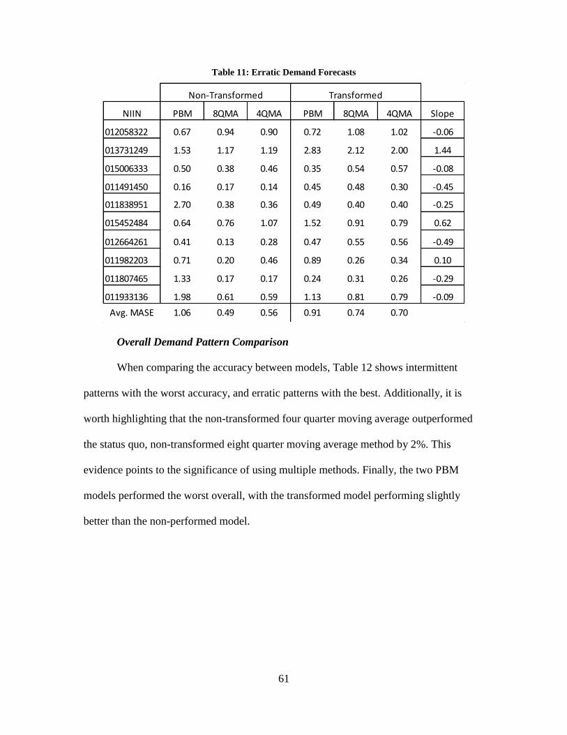
61
Table 11: Erratic Demand Forecasts
Overall Demand Pattern Comparison
When comparing the accuracy between models, Table 12 shows intermittent
patterns with the worst accuracy, and erratic patterns with the best. Additionally, it is
worth highlighting that the non-transformed four quarter moving average outperformed
the status quo, non-transformed eight quarter moving average method by 2%. This
evidence points to the significance of using multiple methods. Finally, the two PBM
models performed the worst overall, with the transformed model performing slightly
better than the non-performed model.
NIIN PBM 8QMA 4QMA PBM 8QMA 4QMA Slope
012058322 0.67 0.94 0.90 0.72 1.08 1.02 -0.06
013731249 1.53 1.17 1.19 2.83 2.12 2.00 1.44
015006333 0.50 0.38 0.46 0.35 0.54 0.57 -0.08
011491450 0.16 0.17 0.14 0.45 0.48 0.30 -0.45
011838951 2.70 0.38 0.36 0.49 0.40 0.40 -0.25
015452484 0.64 0.76 1.07 1.52 0.91 0.79 0.62
012664261 0.41 0.13 0.28 0.47 0.55 0.56 -0.49
011982203 0.71 0.20 0.46 0.89 0.26 0.34 0.10
011807465 1.33 0.17 0.17 0.24 0.31 0.26 -0.29
011933136 1.98 0.61 0.59 1.13 0.81 0.79 -0.09
Avg. MASE 1.06 0.49 0.56 0.91 0.74 0.70
Non-Transformed Transformed

62
Table 12: Demand Pattern Comparison
Now that two PBM forecast methods have been identified as outperforming the
status quo, this next section will test for significance and present a relative comparison.
The first comparison will be testing for a significant difference between the non-
transformed PBM forecast accuracy and the non-transformed eight quarter moving
average method in the smooth demand category. Similar to the approach taken to test for
significance between the mechanical and electrical MASE results, this analysis will also
begin with a test for equal variances. As shown in Table 13, these two samples do not
show evidence to reject the null hypothesis, leading to the conclusion that they do have
equal variances. Finally, the confidence interval shown in Table 14 shows that these are
indeed significantly different in populations.
Table 13: Smooth Demand F-Test for Equal Variances
Table 14: Smooth Demand Test for Equal Means
Pattern PBM 8QMA 4QMA PBM 8QMA 4QMA Avg. MASE
Smooth 1.13 1.19 1.19 1.16 1.32 1.31 1.22
Lumpy 1.70 1.72 1.63 1.53 1.52 1.56 1.61
Intermittent 2.26 1.70 1.61 2.28 1.96 1.97 1.96
Erratic 1.06 0.49 0.56 0.91 0.74 0.70 0.75
Avg. MASE 1.54 1.27 1.25 1.47 1.39 1.39 1.38
Non-Transformed Transformed
F-Test Statistic 0.17
0.05𝛼
1.13
1.19
d.f. 18 Upper Lower
0.50 -0.07 -0.03
t-dist. 0.06
Confidence Interval
𝑠𝑝2

63
The second test for significance is on lumpy demand patterns between the
transformed PBM forecast method and the non-transformed eight quarter moving average
method. As before, this analysis begins with a test for equal variance. Again, as shown in
Table 15, this test concludes that these populations do have equal variances.
Subsequently, the confidence interval shown in Table 16 supports the conclusion that the
transformed PBM method is significantly more accurate than the status quo method.
Table 15: Lumpy Demand F-Test for Equal Variances
Table 16: Lumpy Demand Test for Equal Means
Another way to explain the PBM model’s forecast accuracy relative to the eight
quarter moving average is by determining the percent change in forecast accuracy
between the two. Figure 10 illustrates this well. It can be seen that overall the PBM (both
non-transformed and transformed) performed significantly worse than the baseline.
However, for smooth and lumpy demand patterns there was a significant improvement in
accuracy. Finally, Figure 10 clearly shows that for intermittent and erratic patterns the
PBM well under performs the status quo method.
F-Test Statistic 0.19
0.05𝛼
1.53
1.72
d.f. 18 Upper Lower
2.71 -0.23 -0.14
t-dist. 0.06
Confidence Interval
𝑠𝑝2

64
Figure 10: PBM Forecast Error Relative to Non-Transformed 8QMA
The last area in this analysis explored for possible extrapolation potential was the
potential benefit of using the shear-transformation forecasts over non-transformed
forecasts methods. When aggregating forecast accuracy across all demand patterns Figure
11 shows that while not a significant difference, there is a slight benefit to the non-
transformed forecasts over transformed forecasts.
Figure 11: Non-Transformed Versus Transformed Forecast Accuracy

65
However, in the case of lumpy demand patterns there was a significant difference as
shown in Figure 12. The explanation for this was not transparent, however, this result
was likely influenced by the potential outlier (NIIN 015824217), which as discussed
earlier saw a large error reduction by accounting for the trend in the transformed
methods.
Figure 12: Lumpy Forecast Error
An effort was made to separate all parts with a significant slope versus those will
an insignificant slope to determine if there were additional cases where a trend greatly
influenced the forecast accuracy. Out of the 40 NIINs in this study, only six showed a
positive or negative slope greater than 0.5 demands per period. When looking at those six
NIINs together, the MASE results still showed the non-transformed forecasts with a five
percent better accuracy measure.
Summary
This chapter answered the four investigative questions posed in the introduction.
The first question used the literature review as the substantive evidence that defined the

66
common CBM forecasting methods in academic literature today. Question two sought to
identify data in the USAF’s central data warehouse in an effort to find both event and
condition indicator data. After finding only event data it was recognized that a substantial
loss of CBM capability would be missed without the better quality data. Question three
assessed what could be done with the data obtained, and funneled efforts toward the
PBM. The final investigative question was answered through two separate tests. The first
test looked at evaluating forecast accuracy based on component make-up. It was found
that B-1 parts primarily fell into two categories, mechanical or electrical. This made the
test results less practical than originally thought. The second test established overall
forecast accuracy comparisons between the PBM and an eight quarter moving average.
Then this test addressed differences in accuracy by demand pattern.

67
V. Conclusions and Recommendations
Chapter Overview
The objective of this chapter is to tie together large scale conclusions from this
research effort. Additionally, it quantifies the significance of this research, and frames the
implications of the potential impacts of this research. Then a list of recommended actions
are presented to persuade stakeholders what further measures could advance the impact
this research has on benefiting the USAF. Lastly, a discussion of future research suggests
other follow-on studies.
Conclusions of Research
This research effort began with the ambition to explore the art of the possible, by
capitalizing on the USAF’s data warehouse. A superior competency seemed to divide
new sophisticated forecast methods based on data analytics with the archaic and simple
methods the USAF uses for spare parts. It was this notion that made this topic seem ripe
for improvement.
The first investigative question identified the major CBM forecast methods that
could be used in the application of forecasting aircraft parts. Two particular methods
were recommended as seminal works that should be looked to as baseline models in any
organization using CBM. The first was developed by Jardine et al., (1987). Their method
took a standard hazard function, and updated this distribution based on a particular part’s
condition indicator values. The second method developed by Gebraeel et al., (2005), has
the added benefit of using real-time sensors to update a remaining life curve. Both
instances, along with all of the CBM forecast methods discussed in the literature review

68
are predicated on having information on the condition of a particular part. This is where
the largest set-back in pursuing a true CBM method came.
Investigative question two focused on using the USAF’s data warehouse, Global
Combat Support System-Data Services, to find key data frames that could hold potential
in a CBM format. As thoroughly discussed earlier, a void of condition indicators was
identified. However, recognizing the ample event data, there was still hope for utility in
this data source. Question three then sought to compare what CBM methods could be
applied given the data at hand. A model established by contractors at LMI had proved
very robust in other applications of research. Because of this, their PBM forecast method
looked to be a novel pursuit given only event data.
Question four investigated the statistical evidence comparing the USAF’s primary
forecasts method against a CBM like technique. It did this through two tests. The first test
assessed the PBM’s capacity to differentiate forecast accuracy between electrical and
mechanical components. Though the results of this test proved statistically significant,
the overall method of identifying purely electrical and purely mechanical components
was found to be less substantive than originally hoped. The second test focused on
comparing the PBM against the USAF’s eight quarter and four quarter moving average
forecasts. The overall test results showed that the PBM well under performed the status
quo. However, when broken out by smooth demand, the non-transformed PBM out
performed all other methods. Additionally, for lumpy demand parts, the transformed
PBM method performed significantly better than the standard eight quarter moving
average.

69
Significance of Research
There are three significant aspects of this research. The first shows that a CBM
method using solely event data can be effective. A contribution to academic literature is
that all other CBM forecast methods found required specific beginning and end life cycle
data to form a reliability distribution. A greatly simplified explanation of why the PBM
seems to work is that instead of forming a reliability distribution based on a sample of
failure data, the PBM uses a conditional Bayesian sight-picture to calibrate failure
parameters that in its own way form the reliability distribution. This is done through the
use of a maximum likelihood estimator.
The second significant contribution from this research was found in the second
test of investigative question four. As stated above, there were two specific instances
where the PBM method outperformed the USAF’s primary forecasting method. It was
identified in the introduction that forecast error accounts for $5.5 billion worth of
inventory across all USAF managed parts. Of the smooth and lumpy demand patterns
where the PBM was significantly more accurate, the PBM would have reduced the dollar
value of forecast error on B-1 parts by $12.6 million or effectively 2.46% of error by
dollar value. If this premise was applied across all weapon systems the result would be a
substantially larger dollar value.
The impact of a more accurate forecast method has further implications as well.
When considering a supply chain as a system, the primary methods used to overcome
forecast error are increased safety stock and faster order delivery. To the USAF this
means increased carrying costs, and increased expediting costs. Therefore, the true

70
impact of even minimal forecast improvements would go far beyond accurate
appropriation of funds.
Recommendations for Action
As a result of this research, it is recommended to consider three primary actions.
First, the forecast accuracy results found on smooth and lumpy demand items should be
validated with larger samples and across all airframes. It is possible that forecast accuracy
based on factors of flying hours, number of landings, and number of ground cycles could
have wide ranges. Additionally, other weapon systems may not show a dependent
correlation between the number of flying hours and the number of sorties, thus resulting
in adding the number of sorties as an explanatory variable.
The second recommend action is to suspend the use of demand forecast accuracy
as the central measurement of forecast accuracy in the USAF. As discussed in Chapter II,
there are several critical oversights with this calculation making it unsuitable especially
for intermittently demanded items. Therefore, it is recommended that the USAF adopt the
use of MASE as the primary forecast error calculation it its place. The analytical
performance of this tool is far superior, and should prompt immediate use of MASE.
The last recommendation is to consider an increased use of a four quarter moving
average. Though not thoroughly discussed in the results section, it was shown that the
most accurate forecast method across all demand patterns was the four quarter moving
average. Currently, the USAF uses this forecast method on only 15% of the items it
manages. This research suggests there should be a much larger application of this method
than currently used.

71
Recommendations for Future Research
There are three recommended future topics at the conclusion of this research:
Recommendation 1: Potential conditional information sources
Data use is a widely talked about topic throughout the USAF. Because of this,
several initiatives are in infancy that may solve the missing link the USAF would need to
implement true CBM methods. The first is the F-35’s Automated Logistics Information
System. New processes are improving regularly with the fielding of this technology. This
system is possibly the greatest opportunity for conditional data due to the substantial
number of sensors the jet was designed with. Another opportunity to obtain USAF
conditional data comes from a flight operations data collection system referred to as
Military Flight Operations Quality Assurance (Megatroika, Galinium, Mahendra, &
Ruseno, 2015). At one point in this research effort it seemed possible to obtain raw
sensor data from the government contractor who maintained this system for the B-1
aircraft. However, a substantive wait led to a need to put aside that pursuit. If a researcher
were to pursue this course early and with the right sponsor, then this path may prove
fruitful.
A future project allegedly in work by the Air Force Research Laboratory is a
“Digital Thread Digital Twin” program, however, recent updates on this project were
hard to uncover (Kobryn, 2014). The basic idea is that there is a data surrogate for every
materiel system. This digital twin allows analyst to perform simulated tests or large scale
data analytics such as CBM forecasting.

72
Recommendation 2: CBM Inventory Policy
The second recommendation falls under a very sparsely researched topic. As new
and as limited of an application as CBM is throughout maintenance organizations today,
a notion of a spare parts inventory model based on CBM inputs is even rarer. Picture a
system that would place an order for a part two weeks before a part would fail based on
sensors on a part that would tell the system its diminishment. To some, this would be the
holy grail of inventory management by effectively eliminating the need for safety stock
inventory all together. A novel approach was an age-dependent supply replenishment
policy developed by the U.S. Coast Guard in 2006. When compared to the non-age
dependent policy, the age-dependent policy reduced average total cost by 22%
(Deshpande, Iyer, & Cho, 2006). It should be noted that the Coast Guard’s IT systems
specifically track end items by serial number and by usage, thus allowing such a practice.
Recommendation 3: PBM Sliding Scale Analysis
The final recommended research area is to explore the reliance of the PBM’s
dependence on the sliding scale forecast parameter. As explained in the third chapter of
this report, the PBM scale requires an analyst to forecast both flying hours and a flying
profile ratio between training sorties and combat sorties. The aspect of sliding scale
forecast error was not assessed in this research. Rather, it was assumed that each
forecasted time period’s actual flying profile (known only in hind-sight) was what was
actually predicted. By making this assumption it eliminated variance due to forecasting a
different flying profile than what was executed.
73
Summary
It is the belief of this researcher that CBM has a wide and influential application
throughout the USAF, and should be considered a high priority in the maintenance and
the logistics fields to seek more applications. This research has explored what CBM is
defined as, and how academia views it. Also, this research has addressed previous
initiatives the DoD has engaged in an effort to establish a robust CBM program. After
identifying data collection gaps between where the USAF currently is and where
academia suggests, a novel event data approach to CBM forecast was explored. The
results of this analysis show a limited yet still influential application of the PBM
forecasting method. Finally, the precluding detailed discussion on recommended actions
and recommended future research serve as new opportunities to continually advance the
application of CBM throughout the DoD.

74
Appendix A: Weapon Systems Dash Board
Figure 13: December 2016 Operations Summary Snapshot

75
Appendix B: Diagnostic and Prognostic CBM Summary
Author Article Name Inputs Outputs Technique Significance
Jardine, A., Anderson, P.,
& Mann, D. (1987)
Application of the Weibull
Proportional Hazards Model
to Aircraft and Marine
Engine Failure Data
- Age-dependent baseline hazard function - Condition indicators PHM distribution PHM
Used MLE to find the parameters of Weibull PHM distribution
Moubray, J. (1997)
Reliability-Centered
Maintenance (ed 2)
- Condition indicators - "On-Condition Task" interval P-F Interval P-F Interval
Established framework to estimate TTF
Goode, K., Moore, J., &
Roylance, B. (2000)
Plant machinery working life
prediction method utilizing
reliability and condition-
monitoring data
- Condition Indicators - Weibull parameter estimates TTF distribution P-F Interval
Enhanced Moubray's P-F Interval with a Weibull distribution
Swanson, D. (2000)
A General Prognostic
Tracking Algorithm for
Predictive Maintenance - Condition Indicators Hazard distribution Kalman Filters
Used Kalman Filters to detect changes in indicators
Murray, J., Hughes, G.,
& Kreutz-Delgado, K.
(2005)
Machine Learning Methods
for Predicting Failures in
Hard Drives: A Multiple-
Instance Application
-Self-Monitoring and Reporting Technology (ie. many simultaneous condition indicators)
Fault detection classification
Compared support vector machines, rank-sum, mi-BM (among others)
Proposed efficient/accurate multiple-instance learning algorithm for fault detection
Gebraeel, N., Lawley,
M., Li, R., & Ryan, J.
(2005)
Residual-Life Distributions
From Component
Degradation Signals: A
Bayesian Approach
- Population reliability distribution parameters - Condition Indicators
Residual-life distribution
Bayesian Degradation Signal Model
Real-time sensor based failure model
Wang, W. (2007)
A Two-Stage Prognosis
Model in Condition Based
Maintenance
- Categorical & continuous condition indicators TTF distribution
Discrete/Continuous Hidden Markov Model
Combined continuous and categorical data into state descriptor variable
Tracht, K., Goch, G.,
Schuh, P., Sorg, M., &
Westerkamp, J. (2013)
Failure probability prediction
based on condition
monitoring data of wind
energy systems for spare
parts supply
- SCADA condition Indicators PHM distribution Enhanced PHM
Used SCADA data as covariates in binomial PHM distribution

76
Appendix C: Sliding Scale Equations
Peacetime Average Sortie Duration (ASDPT) =# 𝑃𝑒𝑎𝑐𝑒𝑡𝑖𝑚𝑒 𝑆𝑜𝑟𝑡𝑖𝑒𝑠
# 𝑃𝑒𝑎𝑐𝑒𝑡𝑖𝑚𝑒 𝐹𝑙𝑦𝑖𝑛𝑔 𝐻𝑜𝑢𝑟𝑠
Wartime Average Sortie Duration (ASDWT) =# 𝑊𝑎𝑟𝑡𝑖𝑚𝑒 𝑆𝑜𝑟𝑡𝑖𝑒𝑠
# 𝑊𝑎𝑟𝑡𝑖𝑚𝑒 𝐹𝑙𝑦𝑖𝑛𝑔 𝐻𝑜𝑢𝑟𝑠
Peacetime Average Landings Per Sortie (LPSPT) = # 𝑃𝑒𝑎𝑐𝑒𝑡𝑖𝑚𝑒 𝐿𝑎𝑛𝑑𝑖𝑛𝑔𝑠
# 𝑃𝑒𝑎𝑐𝑒𝑡𝑖𝑚𝑒 𝑆𝑜𝑟𝑡𝑖𝑒𝑠
Wartime Average Landings Per Sortie (LPSWT) = # 𝑊𝑎𝑟𝑡𝑖𝑚𝑒 𝐿𝑎𝑛𝑑𝑖𝑛𝑔𝑠
# 𝑊𝑎𝑟𝑡𝑖𝑚𝑒 𝑆𝑜𝑟𝑡𝑖𝑒𝑠
Predicted Peacetime Flying Hours (PTFH^) = 𝑈𝑠𝑒𝑟 𝑑𝑒𝑓𝑖𝑛𝑒𝑑 𝑓𝑢𝑡𝑢𝑟𝑒 𝑝𝑒𝑟𝑖𝑜𝑑′𝑠 𝑃𝑒𝑎𝑐𝑒𝑡𝑖𝑚𝑒 𝐹𝑙𝑦𝑖𝑛𝑔 %
∗ 𝐹𝑢𝑡𝑢𝑟𝑒 𝑝𝑒𝑟𝑖𝑜𝑑′𝑠 𝐹𝑙𝑦𝑖𝑛𝑔 𝐻𝑜𝑢𝑟𝑠
Predicted Wartime Flying Hours (WTFH^) = 𝑈𝑠𝑒𝑟 𝑑𝑒𝑓𝑖𝑛𝑒𝑑 𝑓𝑢𝑡𝑢𝑟𝑒 𝑝𝑒𝑟𝑖𝑜𝑑′𝑠 𝑊𝑎𝑟𝑡𝑖𝑚𝑒 𝐹𝑙𝑦𝑖𝑛𝑔 %
∗ 𝐹𝑢𝑡𝑢𝑟𝑒 𝑝𝑒𝑟𝑖𝑜𝑑′𝑠 𝐹𝑙𝑦𝑖𝑛𝑔 𝐻𝑜𝑢𝑟𝑠
Predicted Peacetime Cold Cycles (PTCC^) =(𝑃𝑇𝐹𝐻^)
(𝐴𝑆𝐷𝑃𝑇)
Predicted Wartime Cold Cycles (WTCC^) =(𝑊𝑇𝐹𝐻^)
(𝐴𝑆𝐷𝑊𝑇)
Predicted Cold Cycles (CC^) = 𝑃𝑇𝐶𝐶^ +𝑊𝑇𝐶𝐶^
Predicted Peacetime Warm Cycles (PTWC^) = (𝐿𝑃𝑆𝑃𝑇 − 1) ∗ 𝑃𝑇𝐶𝐶^
Predicted Wartime Warm Cycles (WTWC^) = (𝐿𝑃𝑆𝑊𝑇 − 1) ∗𝑊𝑇𝐶𝐶^
Warm Cycles (WC^) = 𝑃𝑇𝑊𝐶^ +𝑊𝑇𝑊𝐶^
Ground Cycles (GC^) = (𝑃𝑜𝑠𝑠𝑒𝑠𝑠𝑒𝑑 𝐻𝑟𝑠𝑡−1 − 𝐹𝑙𝑦𝑖𝑛𝑔 𝐻𝑜𝑢𝑟𝑠𝑡)/24
*Note, this research assumes the user knows the forecast year’s flying profile mix of
PTFH and WTFH. Also, Possessed Hours is assumed to remain constant from last known
year in order to forecast into future years.

77
Appendix D: Demand Pattern Demand Data
Demand
Pattern NIIN-SGM Noun.
2012
Q1
2012
Q2
2012
Q3
2012
Q4
2013
Q1
2013
Q2
2013
Q3
2013
Q4
2014
Q1
2014
Q2
2014
Q3
2014
Q4
2015
Q1
2015
Q2
2015
Q3
2015
Q4
2016
Q1
2016
Q2
2016
Q3
2016
Q4
Smooth 012630536 COMPUTER,F 39 21 27 20 13 13 15 22 19 21 20 18 10 10 21 20 9 8 17 12
Smooth 011433525 CONTROL BO 1 4 8 6 4 2 5 10 1 4 6 9 4 4 9 7 6 4 5 7
Smooth 015097158 ACTUATOR,E 8 6 7 4 4 4 3 4 2 4 2 1 6 5 4 5 2 3 7 6
Smooth 012704772 PCA #3 157 2 8 6 5 8 4 3 1 0 2 8 2 2 2 1 3 3 2 5 3
Smooth 011491452 PUMP,SUBME 9 6 10 7 9 8 8 2 10 13 11 7 6 6 9 9 12 11 14 14
Smooth 011478410 CYLINDER A 3 8 10 8 9 15 8 14 12 15 10 7 9 8 11 7 3 5 1 0
Smooth 012398983 FREQUENCY 13 13 5 10 5 16 13 10 3 6 8 15 16 17 11 5 18 16 10 17
Smooth 013194674 COUPLER,AN 4 3 8 4 4 6 5 3 6 1 6 4 4 1 4 0 1 4 4 0
Smooth 013751527 COMPUTER,F 16 10 20 5 12 3 7 8 9 8 23 5 15 18 6 13 5 2 5 5
Smooth 011829763 INDICATOR, 1 4 4 2 4 5 3 7 5 2 4 6 3 1 1 7 6 2 3 2
Lumpy 013994172 PCA 2 9-S 0 0 0 0 1 1 0 0 0 1 0 0 0 1 0 1 1 0 0 0
Lumpy 015499544 ACTUATOR,E 0 0 0 0 0 0 0 0 0 0 0 0 0 0 2 0 0 0 0 2
Lumpy 011730600 AMPLIFIER, 0 0 0 1 0 0 0 1 0 1 0 0 1 0 0 0 0 0 4 1
Lumpy 013023453 CIRCUIT CA 0 1 1 0 0 0 0 0 0 0 0 1 1 0 0 0 0 1 0 0
Lumpy 015548051 POWER SUPP 0 0 0 0 0 0 0 0 0 0 0 1 0 1 0 0 2 1 0 0
Lumpy 011642197 CONTROL,IN 1 0 3 2 1 2 0 2 1 3 3 1 5 2 0 0 0 1 1 1
Lumpy 015824217 WHEEL,LAND 0 0 0 0 0 0 0 0 0 0 1 8 0 7 64 111 72 44 76 79
Lumpy 015824221 BRAKE,MULT 0 0 0 0 0 0 0 0 0 0 0 1 1 26 12 2 5 4 3 5
Lumpy 011505162 VALVE,HYDR 1 1 2 2 2 0 1 0 0 1 2 0 1 0 3 3 1 1 0 0
Lumpy 012321676 CONTROL UN 2 0 0 1 0 0 0 0 2 0 1 0 0 0 1 0 0 0 0 1
Intermittent 016525025 DRIVE UNIT 0 0 0 0 0 0 0 0 3 3 3 2 2 1 2 4 0 3 2 2
Intermittent 011862809 TANK,HYDRA 0 0 0 0 0 0 0 0 0 0 0 0 0 0 0 1 0 1 0 0
Intermittent 016175632 POWER CONT 0 0 0 0 0 0 0 0 0 2 1 0 0 3 3 7 3 2 2 3
Intermittent 012110135 VALVE,SOLE 0 0 0 0 0 0 2 0 1 1 2 2 2 0 0 0 1 0 0 0
Intermittent 012137727 SWITCH,RAD 0 0 2 2 0 0 0 2 2 1 3 1 0 3 2 2 1 3 0 2
Intermittent 015626911 COMPUTER,F 0 0 0 0 0 1 7 3 2 3 3 5 8 8 3 10 8 5 4 4
Intermittent 016525309 DRIVE UNIT 0 0 0 0 0 0 0 0 2 3 2 2 3 1 2 3 3 3 1 0
Intermittent 011862810 TANK,HYDRA 0 0 0 0 1 0 0 0 0 0 0 0 0 0 0 0 1 0 0 0
Intermittent 011433521 TURBINE,AI 0 0 3 0 1 0 1 0 0 0 4 1 1 2 2 1 1 1 1 0
Intermittent 012112088 VALVE,OXYG 0 0 0 0 0 0 1 0 0 1 0 0 0 0 0 1 0 1 0 1
Erratic 012058322 VALVE,SHUT 3 5 0 1 10 1 3 6 0 2 3 3 1 4 1 4 8 2 5 3
Erratic 013731249 EXTINGUISH 0 10 7 9 25 6 18 20 38 27 4 32 40 34 22 11 3 0 1 0
Erratic 015006333 PCA 11 BL 1 3 1 3 1 0 3 5 2 2 0 2 1 0 1 1 1 2 1 0
Erratic 011491450 PUMP,SUBME 13 3 30 22 5 4 7 14 4 6 2 6 8 4 16 10 8 4 2 5
Erratic 011838951 ANTI-ICE M 6 6 2 3 4 4 15 7 5 5 1 1 2 0 3 4 1 2 2 0
Erratic 015452484 PROCESSOR, 1 2 1 2 2 3 8 8 11 6 7 21 10 3 10 6 15 5 7 7
Erratic 012664261 OSCILLATIN 11 7 9 8 2 2 7 7 1 3 11 1 4 0 2 1 3 2 2 1
Erratic 011982203 CIRCUIT CA 12 3 2 3 5 4 0 0 6 13 15 12 18 0 1 1 8 5 3 3
Erratic 011807465 ELECTRONIC 2 3 8 5 9 3 8 4 3 2 0 2 2 1 2 2 1 1 0 1
Erratic 011933136 CIRCUIT CA 2 4 1 1 4 4 3 4 0 0 3 2 2 1 1 2 3 0 1 1

78
Appendix E: Mechanical and Electrical Demand Data
Part
Category NIIN-SGM Noun.
2012
Q1
2012
Q2
2012
Q3
2012
Q4
2013
Q1
2013
Q2
2013
Q3
2013
Q4
2014
Q1
2014
Q2
2014
Q3
2014
Q4
2015
Q1
2015
Q2
2015
Q3
2015
Q4
2016
Q1
2016
Q2
2016
Q3
2016
Q4
Mechanical 015780463 FLAP,INLET 294 293 218 218 226 247 176 297 125 183 215 165 131 118 156 192 92 98 55 16
Mechanical 013145809 FLAP, DIVE 226 243 191 157 154 166 139 196 165 430 152 161 124 166 58 11 27 11 0 4
Mechanical 011659072 NOSE WHEEL 78 41 29 40 42 23 29 28 16 12 33 16 23 33 31 28 26 20 29 33
Electrical 011491452 PUMP,SUBME 9 6 10 7 9 8 8 2 10 13 11 7 6 6 9 9 12 11 14 14
Electrical 015489586 CIRCUIT CA 34 26 31 26 21 12 3 7 17 23 12 18 7 16 21 18 12 15 2 12
Electrical 014395852 GENERATOR 11 3 11 18 9 11 15 17 20 13 15 23 36 45 12 30 27 22 24 13

79
Appendix F: Quad Chart

80
Bibliography
Aerospatiale Helicopter Corporation. (1980). HH-65A Engine Condition Monitoring
System Specification. Contract Number DOT-CG-80513-A. Grand Prairie, TX.
Air Force Materiel Command. (2011) Requirements For Secondary Items (D200A,
D200N). AFMCMAN 23-1, Interim Change 4. Wright-Patterson AFB, OH.
Air Force Sustainment Center. (2016). Forecast Analysis Comparison Tool Plus User
Manual. Tinker AFB, OK.
Bachman, T. (2007). Reducing Aircraft Down for Lack of Parts with Sporadic Demand.
Military Operations Research, 12 (2), 39–53.
Bachman, T. (2013). Logistics Plans Look Beyond LEO. American Institute of
Aeronautics and Astronautics, Inc., (December).
Boylan, J. (2005). Intermittent and Lumpy Demand: A Forecasting Challenge. Foresight:
The International Journal of Applied Forecasting, 1.
Deshpande, V., Iyer, A., & Cho, R. (2006). Efficient Supply Chain Management at the
US Coast Guard Using Part-Age Dependent Supply Replenishment Policies.
Operations Research, 54 (6), 1028–1040.
Ellis, B. (2008). Conditioned Based Maintenance. The Jethro Project, (November), 1–5.
Gallash, G., Ivanova, K., Rajesh, S., & Manning, C. (2014). Condition Based
Maintenance Technology Impact Study: Assessment Methods, Study Design and
Interim Results. Land Division, Defense Science and Technology Organization.
Fishermans Bend, Victoria, Australia.
Gebraeel, N., Lawley, M., Li, R., & Ryan, J. (2005). Residual-Life Distributions From
Component Degradation Signals: A Bayesian Approach. IIE Transactions, 37 (6),
543–557.
Gehret, G. (2015). Advancing Cost-Effective Readiness by Improving the Supply Chain
Management of Sparse, Intermittently-Demmanded Parts. Ph.D. dissertation, AFIT-
ENS-DS-15-M-256. Air Force Institute of Technology (AU), Wright-Patterson
AFB, OH.
Goldfein, D. (2017). America’s Air Force: Always There. Air Force Public Affairs
Alumni Association. Fairfax, VA. Retrieved March 1, 2017 from
http://www.afpaaa.org/PDF/AlwaysThere.pdf.
Goode, K. B., Moore, J., & Roylance, B. J. (2000). Plant Machinery Working Life
Prediction Method Utilizing Reliability and Condition-Monitoring Data. Institution

81
of Mechanical Engineers, 214 Part E (May 1999), 109–122.
Greitzer, F., Stahlman, E., Ferryman, T., Wilson, B., Kangas, L., & Sisk, D. (1999).
Development of a Framework for Predicting Life of Mechanical Systems: Life
Extension Analysis and Prognostics (LEAP). International Society of Logistics
Symposium. Las Vegas, NV.
Henderson, S., & Kwinn, M. (2005). A Data Warehouse to Support Condition Based
Maintenance (CBM). Operations Research Center of Excellence. Technical Report
DSE-TR-0509 (DTIC ADA434357). West Point, NY.
Hogge, L. (2012). Effective Measurement of Reliability of Repairable USAF Systems. MS
thesis, AFIT/GSE/ENV/12-S02DL. Air Force Institute of Technology (AU),
Wright-Patterson AFB, OH.
Hyndman, R. (2006). Another Look At Forecast-Accuracy Metrics for Intermittent
Demand. Foresight: The International Journal of Applied Forecasting, (4), 43–46.
Jardine, A., Anderson, P., & Mann, D. (1987). Application of the Weibull Proportional
Hazard Model to Aircraft and Marine Engine Failure Data. Quality and Reliability
Engineering International, 3, 77–82.
Jardine, A., Lin, D., & Banjevic, D. (2006). A Review on Machinery Diagnostics and
Prognostics Implementing Condition-Based Maintenance. Mechanical Systems and
Signal Processing, 20 (7), 1483–1510.
Kobryn, P. (2014). Air Force Research Laboratory Digital Thread Update: Why Digital
Thread? Air Force Research Laboratory, Wright-Patterson AFB, OH. Retrieved
March 1, 2017 from
https://adt.larc.nasa.gov/files/2015/03/DigitalThread_for_ERS_Annual_Tech_Meeti
ng_Final_DistA.pdf.
Lowas, A., & Ciarallo, F. (2016). Reliability and Operations: Keys to Lumpy Aircraft
Spare Parts Demands. Journal of Air Transport Management, 50, 30–40.
Lowas III, A. (2015). Improved Spare Part Forecasting for Low Quantity Parts With Low
and Increasing Failure Rates. Ph.D. dissertation. Wright State University, Dayton
OH.
Megatroika, A., Galinium, M., Mahendra, A., & Ruseno, N. (2015). Aircraft Anomaly
Detection Using Algorithmic Model and Data Model Trained on FOQA Data.
Proceedings of the 2015 International Conference on Data and Software
Engineering (ICoDSE), 42-47. IEEE.
Moubray, J. (1997). Reliability-Centered Maintenance (2nd ed.). New York: Industrial
press.

82
Murray, J., Hughes, G., & Kreutz-Delgado, K. (2005). Machine Learning Methods for
Predicting Failures in Hard Drives: A Multiple-Instance Application. Journal of
Machine Learning Research, 6, 783–816.
Navarra, K., Lawton, R., McCusker, S., & Hearrell, N. (2007). An Enterprise Strategy for
Implementing Conditioned-Based Maintenance Plus (CBM+) Research in the
USAF. Proceedings of the 2007 IEEE Aerospace Conference. Paper # 1124.
Oliver, S. (2001). Forecasting Readiness: Using Regression to Predict the Mission
Capability of Air Force F-16 Fighter Aircraft. MS thesis, AFIT/GLM/ENS/01M-18.
Air Force Institute of Technology (AU), Wright-Patterson AFB, OH.
Prajapati, A., Bechtel, J., & Ganesan, S. (2012). Condition Based Maintenance: A
Survey. Journal of Quality in Maintenance Engineering, 18 (4), 384–400.
Reeder, J. (2014). Improving Legacy Aircraft Systems Through Condition-Based
Maintenance: An H-60 Case Study. MS thesis. Naval Postgraduate School,
Monterey, CA.
Silver, B., & Cincotta, K. (2008). Cost Per Flying Hour Analysis, Contingency vs. Peace.
Contract Number GS-00F-0026M, (Order Number GST1104BJ8147). Logistics
Management Institute, McClean, VA.
Slay, F. (1995). Demand Forecasting. Report Number AF401LN2. Logistics
Management Institute, McClean, VA.
Slay, F., & Sherbrooke, C. (1998). Predicting Wartime Demand for Aircraft Spares.
Report Number AF501MR2. Logistics Management Institute, McLean, VA.
Smith, T. (2003). USAF Condition Based Maintenance Plus (CBM+) Initiative. Air
Force Magazine, 84 (5), 102.
Swanson, D. (2001). A General Prognostic Tracking Algorithm for Predictive
Maintenance. Proceedings of the 2001 IEEE Aerospace Conference, 2971–2977.
Swanson, L. (2001). Linking maintenance strategies to performance. International
Journal of Production Economics, 70, 237-244.
Theiss, R. (2013). Identifying Factors that Most Strongly Predict Aircraft Reliability
Behavior. Graduate Research Paper, AFIT-ENS-GRP-13-J-12. Air Force Institute of
Technology (AU), Wright-Patterson AFB, OH.
Tibben-lembke, R., & Amato, H. (2001). Replacement Parts Management: the Value of
Information. Journal of Business Logistics, 22 (2), 149–164.
Tracht, K., Goch, G., Schuh, P., Sorg, M., & Westerkamp, J. (2013). Failure Probability

83
Prediction Based on Condition Monitoring Data of Wind Energy Systems for Spare
Parts Supply. CIRP Annals - Manufacturing Technology, 62 (1), 127–130.
U.S. Air Force. (n.d.). Fact Sheet: Conditioned-Based Maintenance Plus. AcqNotes.
Retrieved March 1, 2017 from
http://www.acqnotes.com/acqnote/careerfields/condition-based-maintenance-
plus%0A.
U.S. General Accounting Office. (1984). The Air Force Can Improve Its Forecasts of
Aircraft Spare Parts Requirements, GAO/NSIAD-85-2. U.S. General Accounting
Office, Gaithersburg, MD. Retrieved March 1, 2017 from
http://www.gao.gov/products/NSIAD-85-2.
U.S. General Accounting Office. (1990). GAO High Risk List. U.S. General Accounting
Office, Washington D.C. Retrieved March 1, 2017 from
http://www.gao.gov/assets/660/659029.pdf.
U.S. Government Accountability Office. (2013). High-Risk Series: An Update, GAO-13-
283. U.S. Government Accountability Office, Washington D.C. Retrieved March 1,
2017 from http://www.gao.gov/assets/660/652133.pdf.
U.S. Government Accountability Office. (2015). High-Risk Series: An Update, GAO-15-
290. U.S. Government Accountability Office, Washington D.C. Retrieved March 1,
2017 from http://www.gao.gov/assets/660/652133.pdf.
U.S. Government Accountability Office. (2016). F-35 SUSTAINMENT: DOD Needs a
Plan to Address Risks Related to Its Central Logistics System, GAO-16-439. U.S.
Government Accountability Office, Washington D.C. Retrieved March 1, 2017 from
http://www.gao.gov/products/GAO-16-439.
Under Secretary of Defense for Acquisition Technology and Logistics. (2012). Condition
Based Maintenance Plus (CBM+) for Materiel Maintenance, DoDI 4151.22.
Retrieved March 1, 2017 from http://dtic.mil/whs/directives/corres/pdf/415122p.pdf.
Van Dyk, S. (2008). Forecasting Flying Hour Costs of the B-1, B-2 and B-52 Bomber
Aircraft. MS thesis, AFIT/GCA/ENV/08-M02. Air Force Institute of Technology
(AU), Wright-Patterson AFB, OH.
Wallace, J., Houser, S., & Lee, D. (2000). A Physics-Based Alternative to Cost-Per-
Flying-Hour Models of Aircraft Consumption Costs. Report Number AF909T1.
Logistics Management Institute, McClean, VA.
Wang, W. (2007). A Two-Stage Prognosis Model in Condition Based Maintenance.
European Journal of Operational Research, 182, 1177–1187.

84
REPORT DOCUMENTATION PAGE Form Approved OMB No. 074-0188
The public reporting burden for this collection of information is estimated to average 1 hour per response, including the time for reviewing instructions, searching existing data sources, gathering and maintaining the data needed, and completing and reviewing the collection of information. Send comments regarding this burden estimate or any other aspect of the collection of information, including suggestions for reducing this burden to Department of Defense, Washington Headquarters Services, Directorate for Information Operations and Reports (0704-0188), 1215 Jefferson Davis Highway, Suite 1204, Arlington, VA 22202-4302. Respondents should be aware that notwithstanding any other provision of law, no person shall be subject to any penalty for failing to comply with a collection of information if it does not display a currently valid OMB control number.
PLEASE DO NOT RETURN YOUR FORM TO THE ABOVE ADDRESS.
1. REPORT DATE (DD-MM-YYYY)
23-03-2017 2. REPORT TYPE
Master’s Thesis 3. DATES COVERED (From – To)
1 Oct 15 – 23 Mar 17
4. TITLE AND SUBTITLE
A Condition Based Maintenance Approach to Forecasting B-1 Aircraft Parts
5a. CONTRACT NUMBER
5b. GRANT NUMBER
5c. PROGRAM ELEMENT NUMBER
6. AUTHOR(S)
DeFrank, Joshua D., Captain, USAF
5d. PROJECT NUMBER
5e. TASK NUMBER
5f. WORK UNIT NUMBER
7. PERFORMING ORGANIZATION NAMES(S) AND ADDRESS(S)
Air Force Institute of Technology
Graduate School of Engineering and Management (AFIT/EN)
2950 Hobson Way
Wright-Patterson AFB OH 45433-7765
8. PERFORMING ORGANIZATION REPORT NUMBER
AFIT-ENS-MS-17-123
9. SPONSORING/MONITORING AGENCY NAME(S) AND ADDRESS(ES)
HAF/A4P
Bill Donaldson, Enterprise Integration Chief Engineer
202 Burlington Rd.
Bedford, MA 01730 (781) 271-3884, (DSN 478-1186 x13884) [email protected]
10. SPONSOR/MONITOR’S ACRONYM(S)
11. SPONSOR/MONITOR’S REPORT NUMBER(S)
12. DISTRIBUTION/AVAILABILITY STATEMENT
Distribution Statement A. Approved for Public Release; Distribution Unlimited.
13. SUPPLEMENTARY NOTES
This work is declared a work of the U.S. Government and is not subject to copyright protection in the United States.
14. ABSTRACT
United States Air Force (AF) aircraft parts forecasting techniques have remained archaic despite new advancements in data
analysis. This approach resulted in a 57% accuracy rate in fiscal year 2016 for AF managed items. Those errors combine for $5.5
billion worth of inventory that could have been spent on other critical spare parts. This research effort explores advancements in
condition based maintenance (CBM), and its application in the realm of forecasting. Then it evaluates the applicability of CBM
forecast methods within current AF data structures. This study found large gaps in data availability that would be necessary in a
robust CBM system. The Physics-Based Model was used to demonstrate a CBM like forecasting approach on B-1 spare parts, and
forecast error results were compared to AF status quo techniques. Results showed the Physics-Based Model underperformed AF
methods overall, however outperformed AF methods when forecasting parts with a smooth or lumpy demand pattern. Finally, it was
determined that the Physics-Based Model could reduce forecasting error by 2.46% or $12.6 million worth of parts in those
categories alone for the B-1 aircraft. 15. SUBJECT TERMS
Condition Based Maintenance, Spare Parts Forecasting, Air Force Parts Forecasting
16. SECURITY CLASSIFICATION OF: 17. LIMITATION OF ABSTRACT
UU
18. NUMBER OF PAGES
97
19a. NAME OF RESPONSIBLE PERSON
Capt Michael P. Kretser, AFIT/ENS a. REPORT
U
b. ABSTRACT
U
c. THIS PAGE
U
19b. TELEPHONE NUMBER (Include area code)
(937) 255-6565, x 4728 ([email protected])
Standard Form 298 (Rev. 8-98) Prescribed by ANSI Std. Z39-18