a context-aware multi-layered sensor network for border ...€¦ · a context-aware multi-layered...

A Context-aware Multi-layered Sensor Networkfor Border Surveillance

Nurali Virani, Pritthi Chattopadhyay, Soumalya Sarkar, Brian Smith,Ji-Woong Lee, Shashi Phoha, and Asok Ray

Abstract Surveillance of the U.S. borders is a crucial challenge to homeland secu-rity. Various initiatives to effectively address this problem with unattended groundsensor (UGS) technology have emerged recently. These initiatives have had limitedsuccess, because UGS have inadequate object and situation assessment capabilitiesdue to their limited processing ability and lack of high-fidelity data. Moreover, theresponse and hence the performance of UGS is significantly affected by environ-mental factors. This chapter focuses on introducing a multi-layered sensor-net ap-proach with context-awareness to effectively address the border surveillance prob-lem. The lowest layer of the proposed network consists of low-fidelity, inexpensiveUGS and higher layers consist of sensors with higher fidelity. Using data-driventechniques, these higher layer sensors can be selectively activated to collect contex-tually relevant data. Depending on their expected contextual value of information,the sensors dynamically form local teams in order to correctly classify border cross-ings with high confidence. The notion of context is explained and mathematicallydefined, and a data-driven technique to develop context evolution models is pro-vided. Some experimental results validating the context-aware classification frame-work using field data are presented. Other research domains which can benefit fromthis work and future research directions are also listed.

Key words: Pattern recognition; Multi-sensor fusion; Context modeling; DDDAS

Shashi Phoha*, Brian SmithApplied Research Lab, Pennsylvania State University, PA, USA, *e-mail: [email protected]

Nurali Virani, Pritthi Chattopadhyay, Soumalya Sarkar, Ji-Woong Lee, Asok RayDepartment of Mechanical and Nuclear Engineering, Pennsylvania State University, PA, USA

1

2 Nurali Virani et al.

1 Introduction to the Data-driven Border Surveillance Problem

The U.S.-Mexico border is approximately 1,950 miles long. The objective of theborder control problem is to deter or detect and apprehend incursions at the im-mediate border or soon after entry. The border is guarded by thousands of borderpatrol agents; however, they cannot themselves completely monitor and prevent il-legal entry on this extensive international border. There are several new initiatives toaddress the above issues by using ground sensors, cameras, radars, mobile surveil-lance systems, and unmanned aerial vehicles (UAV). Use of high-fidelity sensorscan significantly improve situation awareness; however, employing these sensors onthe full stretch of the border for persistent surveillance is impractical due to exces-sive power requirements and financial constraints.

One viable solution is to create a sensor-net by deploying a large number of in-expensive, low power-consuming sensors, which can detect and classify movementsof humans and vehicles as well as communicate the results to a nearby border pa-trolling agent. In such a setting UGS modules with few different sensing modalities,such as acoustic, seismic, infrared, magnetic, and piezoelectric, are typically used.Personnel detection with seismic and passive infrared sensors [15] and footstep de-tection with seismic and acoustic sensors [4, 14] have been reported in literatureto have very good detection performance. One of the major impediments in usingUGS systems for target classification in practical scenarios is that the measurementsof some sensors, for example seismic and acoustic, are severely affected by dailyand seasonal meteorological variations [17]. Since the measurements change withenvironmental factors, the optimal classifiers trained with a specific training datamay not be reliable when those factors change. The desired property in the decision-making framework, which would help these sensor systems overcome this problem,is of context-aware adaptation which is addressed in detail in this chapter.

Attempts have been made to analytically represent the effect of intrinsic contextson the sensors by using physics-based environmental models [30]. Since a largenumber of sensor modules would be deployed, it might not be feasible to obtainall the model parameters (e.g., temperature, wind velocity, soil permeability, soilstiffness, humidity, etc.) for every sensor location. Also, inaccuracies and errors inestimating those parameters might lead to serious concerns of system reliability androbustness. This is the main motivation to develop data-driven approaches for mod-eling of operational contexts for specific sensing modalities. In order to capture theeffects of the contexts on the sensor measurements, a dynamic data-driven approachwas proposed in [29] for sensor networks. Recent work to mathematically formal-ize the notion of context, which would enable machines to model, extract, learn,and perform context-aware interpretation of data is a part of the forward problemof our DDDAS framework, which is presented in detail in Sect. 4. In other words,the forward problem aims to extract and use the knowledge of context to aid in theprocess of converting raw data to actionable knowledge.

The UGS network approach along with contextual adaptation is a practical so-lution. However, the system might not be able to collect enough data to performa classification reliably and/or track the target accurately due to limited sensing

DDDAS for Border Surveillance 3

range and environmental uncertainties. In such a situation, it is desirable to havehigher-fidelity sensors which can be selectively activated to collect more data. Amulti-layered sensor-net framework is envisioned in which higher layers of sens-ing correspond to higher-fidelity, which would give a more reliable classificationin most of the contexts, but need more power and computational effort. The lowerlayer sensors would help to cue the higher layers of sensing to regions of interest.The task of selectively activating higher layers of sensing considering their expectedcontextual information value aims to use the extracted knowledge to adapt the datacollection system itself; hence, it is termed as the inverse problem in this DDDASframework, which is presented in Sect. 5. In this framework, multi-modal sensorsform teams and fuse their measurements or decisions to improve the performanceof the forward problem. This dynamic data-driven multi-layered sensor network isbelieved to be an appropriate solution to address the border surveillance problem.

A typical border surveillance scenario considered in our work is as follows:• Targets: Human(male and female), animals led by human(horse, mule, and don-

key), and all-terrain vehicles(ATV) as shown in Fig. 1.

Fig. 1: Targets: (a) Human; (b) Animal; (c) Vehicle

• Events: Human walking/running individually/in groups, animals with/withoutpayloads, ATVs operating at different speeds.

• Contexts: Terrain, soil type, vegetation, weather, wind, intelligence data, andcommander’s input(e.g., Normal or Alert condition).

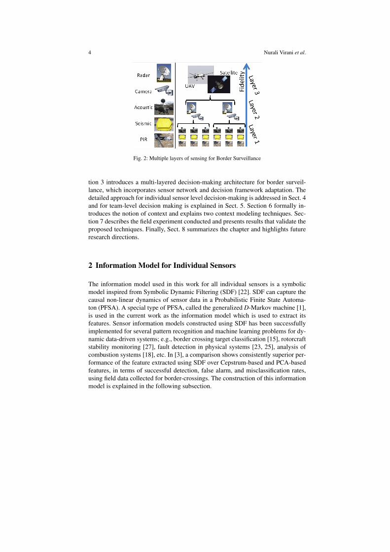
• Sensors: A layered sensor network, as shown in Fig. 2, is to be used in the bor-der surveillance problem. It comprises of UGS at layer 1, high-fidelity sensors,e.g., cameras and radars, form the layer 2, and sensors with possibly the highestfidelity and coverage form layer 3, e.g., UAVs and satellites.

The role of DDDAS for border surveillance is to address two major problems,which can be summarized as follows:

• Forward Problem: To perform context-aware decision-making to improve eventclassification performance.

• Inverse Problem: To optimally adapt the sensor network to collect contextuallyrelevant data to improve event classification, while minimizing cost.

Section 2 explains a sensor information modeling approach which would be usedfor extracting knowledge from raw data for each of the sensors in the network. Sec-


Fig. 2: Multiple layers of sensing for Border Surveillance

tion 3 introduces a multi-layered decision-making architecture for border surveil-lance, which incorporates sensor network and decision framework adaptation. Thedetailed approach for individual sensor level decision-making is addressed in Sect. 4and for team-level decision making is explained in Sect. 5. Section 6 formally in-troduces the notion of context and explains two context modeling techniques. Sec-tion 7 describes the field experiment conducted and presents results that validate theproposed techniques. Finally, Sect. 8 summarizes the chapter and highlights futureresearch directions.

2 Information Model for Individual Sensors

The information model used in this work for all individual sensors is a symbolicmodel inspired from Symbolic Dynamic Filtering (SDF) [22]. SDF can capture thecausal non-linear dynamics of sensor data in a Probabilistic Finite State Automa-ton (PFSA). A special type of PFSA, called the generalized D-Markov machine [1],is used in the current work as the information model which is used to extract itsfeatures. Sensor information models constructed using SDF has been successfullyimplemented for several pattern recognition and machine learning problems for dy-namic data-driven systems; e.g., border crossing target classification [15], rotorcraftstability monitoring [27], fault detection in physical systems [23, 25], analysis ofcombustion systems [18], etc. In [3], a comparison shows consistently superior per-formance of the feature extracted using SDF over Cepstrum-based and PCA-basedfeatures, in terms of successful detection, false alarm, and misclassification rates,using field data collected for border-crossings. The construction of this informationmodel is explained in the following subsection.


2.1 Generalized D-Markov Model for Sensor Information

This section briefly describes the underlying concept of constructing a generalizedD-Markov machine as the sensor information model. While the details are reportedin [1, 22], the underlying concepts are succinctly presented below.

2.1.1 Symbolization of Time Series

Time series data, generated from a physical system or its dynamical model, are col-lected for feature extraction and pattern classification. The ensemble of time seriesdata are symbolized by using a partitioning tool (e.g., maximum entropy partitioning(MEP)) based on a (finite) alphabet Σ whose size (i.e., cardinality) is |Σ |. MEP max-imizes the entropy of the generated symbols, where the information-rich portionsof a dataset are partitioned finer and those with sparse information are partitionedcoarser. Each cell contains (approximately) equal number of data points under MEP.The choice of |Σ | largely depends on the specific dataset and the trade-off betweenthe loss of information and computational complexity.

2.1.2 Generalized D-Markov Machine Construction

A D-Markov machine is a special class of probabilistic finite state automaton(PFSA) [22], where a state is solely dependent on the most recent history of atmost D symbols and the positive integer D is called the depth of the machine. Theunderlying procedure for construction of D-Markov machines consists of two majorsteps, namely, state splitting and state merging. In general, state splitting increasesthe number of states to achieve more precision in representing the information con-tent in the time series, whereas state merging aims to reduce the number of statesby merging states, which do not affect the precision significantly. A combination ofstate splitting and state merging leads to the final form of the D-Markov machine.Once the automaton is constructed, its stationary state probability vector is used asthe low-dimensional feature to represent the time series.

State Splitting1: The number of states of a D-Markov machine of depth D isbounded by |Σ |D. As this relation is exponential in nature, the number of statesrapidly increases as D is increased. However, from the perspective of modeling asymbol string, some states may be more important than others in terms of their em-bedded information contents. Therefore, it is advantageous to have a set of states thatcorrespond to symbol blocks of different lengths. This is accomplished by startingoff with the simplest set of states (i.e., Q = Σ for D = 1) and subsequently split-ting the current state that results in the largest decrease of the entropy rate [1]. Theprocess of splitting a state q ∈ Q is executed by replacing the symbol block q by its

1 This part is intended for the readers interested in the details of the feature extraction procedure,it can be skipped otherwise.


branches as described by the set {qσ : σ ∈ Σ}. Maximum reduction of the entropyrate is the governing criterion for selecting the state to split. In addition, the gen-erated set of states must satisfy the self-consistency criterion, which only permits aunique transition to emanate from a state for each σ ∈ Σ . If δ (q,σ) is not uniquefor all σ ∈ Σ , then the state q is split further.

For construction of PFSA, each element π̂(σ ,q) of the estimated morph matrixΠ̂ is calculated by frequency counting as the ratio of the number of times, N(qσ),the state q is followed by the symbol σ and the number of times, N(q), the state qoccurs i.e.,

π̂(q,σ), 1+N(qσ)

|Σ |+N(q)with ∑

σ∈Σπ̂(σ ,q) = 1 (1)

State Merging1: After state splitting is performed, the resulting D-Markov ma-chine is a statistical representation of the symbol string under consideration. De-pending on the choice of alphabet size |Σ | and depth D, the number of states aftersplitting may run into hundreds. The motivation behind the state merging is to re-duce the number of states, while preserving the D-Markov structure of the PFSA.This process may cause the PFSA to have degraded precision due to loss of infor-mation. The state merging algorithm aims to mitigate this risk.

Let K1 = {Σ ,Q1,δ1,π1} be the split PFSA, and let q,q′ ∈ Q1 be two states thatare to be merged together. In order to proceed with the merging of states q and q′,an equivalence relation is imposed between q and q′, denoted as q ∼ q′; however,the transitions between original states may not be well-defined anymore, in the fol-lowing sense: there may exist σ ∈ Σ such that the states δ1(q,σ) and δ2(q′,σ) arenot equivalent. In essence, the same symbol may cause a transition to two differentstates from the merged state {q,q′}. As the structure of D-Markov machines doesnot permit this ambiguity of non-determinism [22], the states δ1(q,σ) and δ2(q′,σ)are also required to be merged together, i.e., δ1(q,σ) ∼ δ2(q′,σ). Therefore, thesymbol σ will cause a transition from the merged state {q,q′} to the merged state{δ1(q,σ),δ2(q′,σ)}. This process is recursive and is performed until all state tran-sitions are unambiguous.

Now the split PFSA K1 = {Σ ,Q1,δ1,π1} is merged to yield the reduced-orderPFSA K2 = {Σ ,Q2,δ2,π2}, where the state-transition map δ2 and the morph func-tion π2 for the merged PFSA K2 is defined on the quotient set Q2 , Q1/ ∼, and[q] ∈ Q2 is the equivalence class of q ∈ Q1. Then, the associated morph function π2is obtained as:

π2 ([q],σ)≈∑q̃∈[q] π̂1(q̃,σ)× P̂1(q̃)

∑q̃∈[q] P̂1(q̃)(2)

By construction, δ2 ([q],σ) is naturally equal to [δ1(q,σ)]. The similarity of twostates, q,q′ ∈ Q, is measured in terms of morph functions (i.e., conditional probabil-ities) of future symbol generation as the distance (M (q,q′), ℓ1-norm based distancefunction) between the two rows of the estimated morph matrix Π̂ corresponding tothe states q and q′. First, the two closest states (i.e., the pair of states q,q′ ∈Q havingthe smallest value of M (q,q′)) are merged by creating the equivalence relation as


described earlier. Subsequently, distance Ψ(·, ·) [1] of the merged PFSA from theinitial symbol string is evaluated. If Ψ < η where η is a specified threshold param-eter, then the machine structure is retained and the states next on the priority list aremerged. On the other hand, if Ψ ≥ η , then the process of merging the given pair ofstates is aborted and another pair of states with the next smallest value of M (q,q′)is selected for merging. This procedure is terminated if no such pair of states exist,for which Ψ ≥ η .

After the D-Markov machine is constructed, the stationary state probability vec-tor is computed in the following way. Similar to (1), each element of the stationarystate probability vector P(q) is estimated by frequency counting as

P̂(q), 1+N(q)|Q|+∑q′∈Q N(q′)

∀q ∈ Q. (3)

The stationary state probability vector is used as the low-dimensional feature repre-senting the associated time series for the extraction of actionable intelligence. Thenext section introduces the formulated multi-layered decision-making architecturefor addressing the border surveillance problem.

3 Multi-layered Decision-making Architecture for BorderSurveillance

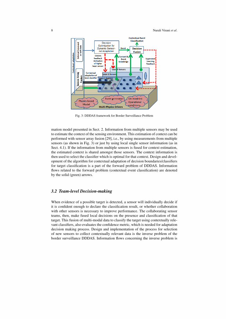
A multi-layered sensor network architecture for border surveillance is illustrated inFig. 3. In a multi-layered sensor network, the sensing agents have several possi-ble actions to choose from. These actions possibly include various capabilities: toreport the estimated event data to a border patrolling agent/commander, to changeclassification framework (e.g., decision boundaries and feature extraction schemes),to change measurement system parameters (e.g., sampling frequency, sample size,etc.), to collaborate with other ground sensors in order to improve classification per-formance by sensor fusion, and to request for more accurate and more expensivehigher layer sensors to collaborate in the situation and object assessment process.Some of these actions are taken by an individual sensing agent, while others aretaken by a team of sensors. The decision-making architectures for individual andteam of sensors are introduced in Sect. 3.1 and 3.2, respectively. The proposedarchitecture aims to augment all decision-makers with the capability of context-awareness; this notion is introduced in Sect. 3.3.

3.1 Individual Sensor-level Decision-making

Primary sensing activity occurs in the Layer 1 sensors, envisioned as the suite ofmulti-modal UGS. Sensed data from individual sensors is modeled with the infor-


Fig. 3: DDDAS framework for Border Surveillance Problem

mation model presented in Sect. 2. Information from multiple sensors may be usedto estimate the context of the sensing environment. This estimation of context can beperformed with sensor array fusion [29], i.e., by using measurements from multiplesensors (as shown in Fig. 3) or just by using local single sensor information (as inSect. 4.1). If the information from multiple sensors is fused for context estimation,the estimated context is shared amongst those sensors. The context information isthen used to select the classifier which is optimal for that context. Design and devel-opment of the algorithm for contextual adaptation of decision boundaries/classifiersfor target classification is a part of the forward problem of DDDAS. Informationflows related to the forward problem (contextual event classification) are denotedby the solid (green) arrows.

3.2 Team-level Decision-making

When evidence of a possible target is detected, a sensor will individually decide ifit is confident enough to declare the classification result, or whether collaborationwith other sensors is necessary to improve performance. The collaborating sensorteams, then, make fused local decisions on the presence and classification of thattarget. This fusion of multi-modal data to classify the target using contextually rele-vant classifiers, also evaluates the confidence metric, which is needed for adaptationdecision making process. Design and implementation of the process for selectionof new sensors to collect contextually relevant data is the inverse problem of theborder surveillance DDDAS. Information flows concerning the inverse problem is


shown in dashed (red) arrows. The sensors used in team formation can be UGSoperating in low-power detection-only mode or can be higher layer sensors, whichcollect high-fidelity data to improve classification performance. Information regard-ing both context and target classification, including confidence metrics, are used inmaking decentralized network adaptation decisions. For clarity, the decision opti-mization (for dynamic sensor-net adaptation) block and decision-fusion block areshown separately in Fig. 3, but in an operational system, both blocks are envisionedto be embedded in the processing units of the individual sensors. The processingcan be carried out by a dynamically selected team leader or sensor cluster head. Theimplementation of the adaptation decision from the sensor team can be subjected toapproval from appropriate authorities.

3.3 Context-aware Decision-making

The DDDAS for border surveillance can address the problem more effectively, ifalgorithms for context-awareness and context-aware adaptation are developed andimplemented for the sensor system. In other words, the performance at the Level1 (Object Assessment) of the DFIG (Data Fusion Information Group) data fusionmodel [5] can be improved by using the output of Level 2 (Situation Assessment).

In order to implement context-awareness for automated systems, it is first neces-sary to precisely define the concept of “context”. One possible definition, providedby Dey et al. [10], is as follows: “Context is any information that can be used tocharacterize the situation of an entity. An entity is a person, place, or object thatis considered relevant to the interaction between a user and an application, includ-ing the user and applications themselves.” Their work focused specifically on theimplementation of context-aware features for design applications in hand-held de-vices, which could be effectively customized to the user’s current situation by usingimplicitly sensed context. Blasch et al. [6] made an extensive survey of contextualtracking for information fusion. Shi et al. [26] performed vehicle detection fromwide area motion imagery by extracting contextual information about roads fromvehicle trajectories and fed back this information to reduce false alarms. Contextdue to the target itself may refer to pose change, deformation, etc. and due to ex-ternal factors such as changes in illumination, viewpoint, occlusions, etc. Oliva etal. [20] did an extensive review of work done on effects of context on object recog-nition by humans, methods of learning of contextual information by the human brainand the mechanism of contextual analysis by humans. Elnahrawy [11] have definedcontext in terms of values of neighboring sensing nodes in sensor networks and thepast history of measurements of the sensor, which can be used to predict the nextsensor reading. The notion of context in the DDDAS framework presented here,differs from those mentioned above in two specific ways:

1. The context is required to be machine-understandable in order to allow machinesto autonomously extract it from sensor data and then use it to improve decisionsand to adjust the sensing mechanisms.


2. Two different types of contexts are identified based on their influence on thesensor data:

• Intrinsic Context: Factors that directly influence the sensor measurements fora particular event are called the intrinsic context. For example: Changes insoil stiffness due to precipitation affect seismic sensor response for a bordercrossing event [17]; changes in lighting conditions affect camera pictures of aperson for identity verification.

• Extrinsic Context: Factors that do not affect the sensor measurements forany particular event, but influence the interpretation of sensor data, formthe extrinsic context. For example: Intelligence information about a possi-ble smuggling-related border crossing; changes in commander’s input (e.g.,switch to alert from normal mode).

The definitions for these different types of context and mathematical formalizationof the notion of context is given in Sect. 6. A context-aware system has the ability toextract/learn context from available data. The context-aware decision-making pro-cess uses these context models to enhance the system’s decision-making capabilityand possibly improve its performance.

In many cases, the sensors in the second and third layers will be more reliableand expensive sensors than those in the ubiquitous first layer. If those higher layersensors have been called into the sensor team and credible event classification hasbeen performed, the final classification result can be used as supervised trainingfeedback to update the classifiers of all the lower layer sensors. In Fig. 3, this feed-back is shown as dotted (red) arrow. In this border surveillance DDDAS frame-work, each feedback path operates at a different time-scale with a dedicated pur-pose; namely, contextual adaptation of classifiers, adaptation of the measurementsystem, and supervised learning feedback. The technical details of the above threeSub-sects. 3.1, 3.2, and 3.3 are explained in detail in Sect. 4, 5, and 6, respectively.

4 Decision-making with Individual Sensor

The process of using knowledge, i.e., features, for extracting actionable intelligence,i.e., classification of the target, is explained in this section. This section will ad-dresses a local target classification decision-making process using context-basedclassifiers.

4.1 Contextual Classification

Context and events both affect the sensor measurements. If the effect of contexton the sensors measurements for the same event is much smaller than the effect of


different events under the same context, then, practically there might not be any clas-sification performance improvement by using the knowledge of context. There aremany realistic problems in which this is not the case, so the effect of different con-texts is either comparable or larger than that of the different events. In such cases, itis beneficial to extract the knowledge of context and use it to improve event classifi-cation performance. The technique developed (to extract context from sensor data)and used in this work involves, first classifying the features extracted from time se-ries to identify context and then, using the classifier which improves classificationperformance in the known context. Not only the decision boundary/classifier, butalso, the feature extraction scheme can be adapted according to the identified con-text. Traditionally, a classifier is defined as a function which maps a feature spaceinto a finite set. In [29], the term context-based classifier was introduced as follows:

Definition 1. (Context-based Classifier) Let C be the set of contexts, Ψ be the set offeatures, and X be the (finite) set of classes. Then, a function A : C ×Ψ → X is saidto be a context-based classifier, if ∀ c ∈ C , ∀ P ∈Ψ , A(c,P) ∈ X . In other words,A(c, ·) is a classifier ∀ c ∈ C .

The exact procedure for construction of the set of contexts C is explained in Sect. 6.These classifiers take input of feature and context and give output as the event classof the feature under the given context. The context-based classifiers essentially im-plement a dynamic classifier selection framework in a systematic way.

This section explained a contextual classification approach. The next section willintroduce the problem of dynamic sensor team formation and team-level decisionfusion for target classification.

5 Team Formation and Team-level Decision-making

The inverse problem aims to carry out the decision optimization for dynamic sensornetwork adaptation. In order to fulfill this objective by sensor team formation, a dy-namic programming approach is proposed. An example is presented to explain theproblem. In Fig. 4, a sensor-net has UGS (A, B, C, and D) and Radar (E); a UAV(F) can be activated for surveillance in that region. A “target” is going through thesensor-net (dotted arrow) and sensor C first detects the target. Sensor C then makesa target classification decision and computes the associated cost for the current teamconfiguration consisting of sensor C only. It also computes the expected cost foreach new possible team configuration (e.g., {C,B}, {C,E}, and {C,F}). Then thesensor, which minimizes the expected cost (determined by the value of informationand the cost of operating an additional sensor) is activated. If the additionally se-lected sensor is a ground sensor (e.g., B), then it shares the measurement with theother team member and the target classification decision, along with the confidencescore, is updated accordingly. If the selected sensor is a higher layer sensor (e.g.,E), then information of target location from lower layer sensors is used to cue thehigher layer sensor, and new measurements are collected. This sensor selection pro-


Fig. 4: Formation of local sensor teams

cess repeats and the team of sensors evolves over time in order to classify and trackthe target in an optimal manner.

The ground sensors often have small operation cost and insufficient classifica-tion ability between a few target classes. On the other hand, higher layer sensorsare expected to have high operation cost, but would have more reliable classifica-tion performance in several contexts. A unified framework for optimally trading offclassification performance against sensor activation/operation cost is presented inthis section. A simplified version of this problem is first formulated, in which thereis only one potential location, and multiple sensors can be activated to get more in-formation about the target in that location. Further extensions to this framework arementioned in Sect. 5.2.

5.1 Problem Formulation and Solution Approach

A random variable X , which represents a target class at a fixed location, takes valuesin a finite hypothesis set H = {0,1, . . . ,M − 1}. Let S = {1,2, . . . ,N} be the set ofavailable sensors. The prior probability of X = x is p(x) for x ∈ H. Conditioned onX = x ∈ H, the measurement Yi sampled from sensor i has the probability densitypi(y | x) at Yi = y ∈ Rni , where ni denotes the fixed sample size of sensor i. Condi-tioned on X , the measurements Y1, . . . , YN are assumed to be mutually independent.

A dynamic data-driven sensor selection procedure is as follows. Initially, a deci-sion of whether to declare the value of X based solely on the prior distribution p(·)of X or not has to be taken. In the sensor network, UGS sensors will initially beactivated, but for the sake of generality, assume sensor i was activated first and itsmeasurement Yi = yi was obtained. Again, a decision has to be made whether todeclare the value of X based on the posterior distribution p(· | Yi = yi) of X , or todefer the classification decision to after selecting an additional sensor and samplingits measurement. In this manner, a subset C ⊂ S of sensors are selected, incurringan observation cost ∑i∈C ci, and a terminal decision on the value of X is made based


on the posterior distribution p(· | Yi = yi, i ∈ C) of X , where an incorrect terminaldecision incurs an additional cost dC.

Suppose all N sensors have been selected and the posterior distribution of Xconditioned on Yi = yi for all i ∈ S is given by p = (p0, p1, . . . , pM−1), where px =p(x | Yi = yi, i ∈ S) for x ∈ H. Then the optimal decision on the value of X is x̂ =argmaxx∈H px. In addition to the observation cost ∑i∈S ci, this decision incurs anexpected cost VS(p), given as follows:

VS(p) = dS(1−max

x∈Hpx). (4)

Suppose a subset S \{ j} of sensors (i.e., all sensors except for sensor j) have beenselected and the posterior distribution of X conditioned on Yi = yi for all i ∈ S\{ j}is given by p = (p0, p1, . . . , pM−1), where px = p(x | Yi = yi, i ∈ S \ { j}) for x ∈H. The sensor team has to determine whether to declare the value of X based onthe measurements of the current team or to add sensor j before making a terminaldecision. Denoting the conditional expectation given Yi = yi, i ∈ S \ { j}, by Ep[·],the optimal expected cost in this case, in addition to the observation cost associatedwith the selected sensors S\{ j}, is as follows:

VS\{ j}(p) = min{

dS\{ j}(1−max

x∈Hpx), c j +Ep

[VS(Φ j(p,Yj)

)]}= min

{dS\{ j}

(1−max

x∈Hpx)

︸︷︷︸Do not add sensor j

, c j + ∑x∈H

∫VS(Φ j(p,y)

)p j(y | x)px dy︸︷︷︸

Add sensor j

},

where

Φ j(p,y) =(

p j(y | 0)p0

∑x∈H p j(y | x)px,

p j(y | 1)p1

∑x∈H p j(y | x)px, . . . ,

p j(y | M−1)pM−1

∑x∈H p j(y | x)px

)(5)

is the posterior distribution p = (p0, p1, . . . , pM−1) of X updated by the additionalmeasurement Yj = y for y ∈ Rni . If VS\{ j}(p) = dS\{ j}

(1 − maxx∈H px

), then the

optimal team decision is to make the terminal decision x̂ = argmaxx∈H px withoutadding sensor j. On the other hand, if VS\{ j}(p) = c j +Ep

[VS(Φ j(p,Yj)

)], then

the optimal decision is to add sensor j (i.e., to use all sensors) before making theterminal decision.

Suppose now that an arbitrary, proper subset C ( S of sensors have been selectedand the posterior distribution of X conditioned on Yi = yi for all i∈C is given by p=(p0, p1, . . . , pM−1), where px = p(x | Yi = yi, i ∈C) for x ∈ H. One has to determinewhether to stop adding sensors and declare the value of X or to select an additionalsensor from S\C. Denoting the conditional expectation given Yi = yi, i∈C, by Ep[·],the optimal expected cost at this stage (in addition to the observation cost ∑i∈C ci) isthen given as follows:


VC(p) = min{

dC(1−max

x∈Hpx)

︸︷︷︸Stop adding sensors

, c j +Ep[VC∪{ j}

(Φ j(p,Yj)

)]︸︷︷︸Add sensor j

, j ∈ S\C}. (6)

If VC(p) = dC(1−maxx∈H px

), then the optimal decision at this stage is to stop

adding sensors and make the terminal decision x̂ = argmaxx∈H px. The x̂ computedhere has fused the measurements from several multi-modal sensors in C and hasevaluated the value associated with the decision of the team as VC(p). On the otherhand, if VC(p) = c j +Ep

[VC∪{ j}

(Φ j(p,Yj)

)]for some j ∈ S \C, then the optimal

decision is to add sensor j to the existing team.Lastly, suppose that the system is at the initial stage, where no sensor has been

selected. Then, denoting the prior distribution of X by p = (p0, p1, . . . , pM−1), theoptimal cost is

V∅(p) = min{

d∅(1−max

x∈Hpx)

︸︷︷︸Do not use sensors

, ci +E[V{i}

(Φi(p,Yi)

)]︸︷︷︸Select sensor i

, i ∈ S}, (7)

where E[·] denotes the (unconditional) expectation (based solely on the prior p).Note that, while the very first sensor is selected based solely on the prior distributionof X , the selection of the other sensors depends on the measurements. The expectedoverall cost incurred by the optimal sensor selection scheme is equal to V∅(p).

This approach implicitly defines a value associated with the information obtainedfrom a sensor and uses it to make an adaptation decision. The expected value ofinformation EV I( j;C) defined for sensor j, when it is added to the team C, is givenby the relation

EV I( j;C) =VC(p)−E[VC∪{ j}

(Φ j(p,Yj)

)| Yi = yi, i ∈C

], (8)

where E[·] denotes the expectation and p = (p0, p1, . . . , pM−1) with px = P(x | Yi =yi, i ∈ C). This EV I( j;C) is the expected marginal contribution of sensor j to thevalue of the team C, when it is added to that team. If the cost of installation, activa-tion, and operation of sensor j given by c j > EV I( j;C), then the sensor would notbe added to the team. In fact, the sensor j (with j ∈ S \C) with the highest residualEV I( j;C)− c j is added to the team, if the residual is positive; otherwise, the teamremains unchanged. This evaluation is done via dynamic programming (6).

5.2 Extension of Formulation

The proposed framework is general enough to be used for decision level informa-tion fusion, instead of the feature/measurement level fusion for the sensor networkadaptation problem. The decision level fusion approach, where the sensor measure-ment yi is replaced with the classification decision x̂i of sensor i, can potentiallysuffer significant information loss. On the other hand, for a large sample size, it is


infeasible to compute expectations over the set of all measurements. Thus, a fusionalgorithm, which uses most of the collected information and yet is computationallyefficient, is currently being developed.

It is understood that, in some contexts, lower layer sensors might have good re-liability and higher layer sensors can be very unreliable. For example, an acousticsensor on a calm summer day might give good human-vehicle classification results;a camera might not be useful in poor visibility conditions. This effect of intrinsiccontext can be included in the framework by means of contextual observation den-sities P(X | Y,C ) and contextual classification performance P(X̂ | X ,C ), where X ,X̂ , Y , and C are random variables for target class, estimated target class, sensormeasurement, and context state, respectively.

The system behavior should adapt to the extrinsic context. While the target classpriors should be adjusted to incorporate intelligence information, the willingness topay more cost to avoid a missed detection during a critical situation must also beincorporated. The expected cost function given in (4), in general, can be made non-linear to represent a particular desired behavior of the team, such as willingness orreluctance to collaborate depending on the extrinsic context. These additions to theframework will enable the system to perform context-aware sensor network adapta-tion along with the capability of context-based classification.

There are several other means to adapt the measurement system to improveclassification performance, such as adaptation of sensor data length, sampling fre-quency, etc. The techniques developed in [24] for transient time series analysis givea decision along with a probability distribution over the set of classes. This dis-tribution can be used in the sequential hypothesis testing framework along with asuitably chosen threshold to determine whether larger sample sizes should be usedfor improved confidence in classification. This technique would consider the cost ofsampling, excess computation, value of information of the new data, and extrinsiccontext-dependent penalties of Type I and Type II errors to choose the threshold.

6 Context-aware Decision-making

In the this section, the notion of context, which has been used throughout this chap-ter, is mathematically formalized. This formalism aims to enable machines to extractand model the operational context. Once, context is modeled, both the forward prob-lem and the inverse problem will use the knowledge of context to improve systemperformance. The mathematical formalism of context provided ahead is general inorder to enable its use with any data-driven system. A more detailed explanation ofthe concepts introduced in this section has been provided in [21].


6.1 Context Learning and Evolution Modeling

The aim of modeling context and its evolution has been addressed by the re-search community using physics-based modeling [30] as well as data-driven mod-eling, to understand the environment and its impact on sensor data. The data driventechnique proposed in this work adopts a generalized D-Markov machine model-ing approach [1, 22] (Sect.2.1). If the space of feature vectors extracted from mea-surements of each sensing modality can be partitioned (i.e., mutually exclusive andexhaustive division of space) and each of the finitely many partitions is assigned asymbol, then a set of symbols called the alphabet is obtained. The sensor data inthe fast time scale is used to generate the features, while the time series of featuresfrom that sensor data has a slower time scale. Each of the features in that time seriesis assigned a symbol according to the partition to which it belongs in the featurespace. Thus, from a time series of features, a symbol sequence is obtained. In orderto model the evolution of the features, a generalized D-Markov machine model iscreated from the symbol sequence (as explained in Sect. 2.1.2). The partitioning ofthe feature space can be accomplished in several ways and choosing an appropriateway, which gives meaningful and robust features, is the key aspect in the modelingof context evolution. If each symbol in the alphabet is representative of the differ-ent distinguishable factors affecting the sensing modalities, then the symbol and thealphabet are called the context symbol and context alphabet, respectively. The corre-sponding generalized D-Markov model is called the context evolution model. Everystate of the generalized D-Markov model of context evolution is a string of less thanor equal to D number of context symbols and is called a context state.

Two different techniques to obtain the context alphabet are proposed in this workfor cases in which the factors affecting the sensing modality are known and canbe simulated or otherwise. Context alphabet construction can be addressed in thefollowing two ways:

1. Supervised Modeling: In some application areas, all relevant factors which sig-nificantly affect the data are known and these factors can be individually appliedto the system (probably in a controlled environment). It is desired to use thisknowledge in training and improve system performance. This technique of mod-eling context with knowledge of the relevant factors known a priori is a form ofsupervised modeling.

2. Unsupervised Modeling: In most application areas, the factors affecting the dataare either not known a priori or cannot be individually applied in a controlled en-vironment. Such systems need to learn the relevant factors, during in-situ trainingby using unsupervised learning algorithms. This technique of modeling contextis a form of unsupervised modeling.

Both of these approaches are used to obtain a set of labels for distinguishablefactors affecting the sensor data, i.e., a context alphabet. Sect. 6.2 will mathemat-ically define the two different types of context. Sect. 6.3 and 6.4 address the twoabove-mentioned techniques for context alphabet construction in detail.


6.2 Mathematical Definition of Context

Let S be a nonempty finite set of sensing modalities and X be a random variable,which takes values in a finite set H of hypotheses of random events. Let s ∈ S be asensing modality, that, is used to observe a random event x ∈ H and let Y (s) be arandom vector associated with the measurement of sensor s, which is used to classifythe event of interest x.

Definition 2. (Context Elements) Let L (s) be a non-empty finite set of labels. Eachelement of L (s) is called a context element. Every context element is a physicalphenomena (natural or man-made), which is relevant to the sensing modality usedto observe an event of interest. It is assumed, that the elements of the set L (s) havebeen listed in such a way, that no two elements can occur simultaneously.

The assumption in construction of L (s) is not restrictive. If it is possible for fewcontext elements (say, l, m and n) to occur together, then, a new context element(sayk) representing l, m, and n occurring together is added to L (s) and the extensionof L (s) is obtained. Further computation would be done using this extension. LetP(Y |X , l) be the contextual observation density of sensor measurements of modal-ity s ∈ S for event X , under a given context l ∈ L (s). These observation densitiesmodel the likelihood of a particular measurement for an event with context elementl. Classification of events would be performed using features extracted from themeasurements, so it is convenient and practical to construct observation densitieswith low dimensional features, instead of the actual measurements. Using the intu-ition, that the context elements in an intrinsic subset may probabilistically affect themeasurement Y associated with an event X , whereas an extrinsic context does notaffect the conditional distribution P(Y |X), a definition is formalized as follows.

Definition 3. (Extrinsic and Intrinsic Subsets of Contexts) A nonempty set C̃ ⊆L (s) is called extrinsic relative to an event X and the associated measurement Y , if

∀ l, l̃ ∈ C̃ , P(Y |X , l) = P(Y |X , l̃).

A nonempty set C̃ ⊆ L (s) is called intrinsic relative to an event X and the asso-ciated measurement Y , if

∃ l, l̃ ∈ C̃ such that P(Y |X , l̃) ̸= P(Y |X , l).

The models for intrinsic context evolution can be autonomously extracted bythe sensors using the data-driven approaches presented here. Two context alphabetconstruction approaches to build the D-Markov models for context evolution aregiven in the following two sub-sections.


6.3 Supervised Modeling of Context

Following Definition 2, observation densities P(Y (s)|x, l) ∀x ∈ H, ∀ l ∈ L (s), canbe constructed, if several measurements Y are collected for an event x ∈ H underthe same context element l ∈L (s). If the observation densities are overlapping andvery close, then, those context elements would have nearly the same effect on thesensor data. Sets of context elements which are approximately indistinguishable canbe constructed for a given threshold parameter ε > 0 and a metric d(·, ·) on the spaceof observation densities using the following definition.

Definition 4. (Context Alphabet and Context Symbol) Let C(s,x) be a set cover ofL (s) for each modality s and event x. Then, C(s,x) is called a context alphabetand a (non-empty) set c(s,x) ∈ C(s,x) is called a context symbol provided that thefollowing properties hold:

1. c(s,x) ={

l,m ∈L (s) : d(P(Y |x, l),P(Y |x,m))< ε}

. Then, the observation den-sity P(Y |x, l) ∀ l ∈ c is denoted as P(Y |x,c).

2. The set c(s,x) is maximal, i.e., it cannot be augmented by including anotherelement l ∈ L (s).

The construction of a context alphabet from the training dataset is reduced tothe standard maximal clique listing problem in graph theory. A maximal clique isa complete subgraph, that, cannot be extended by including one more adjacent ver-tex. In the maximal clique listing problem, the input is an undirected graph, andthe output is a list of all its maximal cliques. At first, a complete weighted graphG with context elements as the vertices and the distance between any two contex-tual observation densities as the weight of the respective edge is constructed usingall context elements in L (s) and a suitable metric d(·, ·). Then, all edges whoseweight is larger than the threshold parameter ε are deleted to obtain undirectedgraph G′. Finally, the maximal clique listing problem for the undirected graph G′

is solved using algorithm in Remark 1. If a symbol is assigned to each maximalclique, the set of all symbols associated with the maximal cliques is the contextalphabet, because a maximal clique in G′ represents all possible context elementswhose observation densities are mutually close together or the observations of thechosen modality are mutually indistinguishable. This procedure offers to select thethreshold parameter ε , which can be used to trade-off between robustness and mod-eling accuracy/performance. If the threshold parameter ε is too large, there wouldbe just one context, the complete graph would be the only maximal clique. On theother hand, if ε is too small, during thresholding all the edges will be deleted, andall singleton contexts would be obtained, i.e., the isolated vertices in the graph. Theexact mechanism to choose ε is application specific and needs to be investigated.

Remark 1. (Algorithms for Listing all Maximal Cliques) Enumeration of maximalcliques in an undirected graph has been widely researched topic in the domain ofgraph theory and combinatorics [2, 7, 8]. The popular Bron-Kerbosch algorithm [7]is efficient in the worst-case sense with a running time of O(3n/3). The problem


is NP Complete, so any known exact algorithms have exponential time complex-ity. The application targeted in this paper will usually be reduced to a small graph(< 100 vertices), so time complexity is not a major concern. This work uses the al-gorithm mentioned in [28], which is a variant of original Bron-Kerbosch Algorithm.

6.4 Unsupervised Modeling of Context

In general, the context under which the data is collected is unknown a priori andin many cases, multiple factors affect the data together. Hence, some context infor-mation needs to be extracted autonomously from the sensor data. For a given event,the feature vectors extracted from repeated experiments, under the same context areexpected to be close to each other in the feature space. With this intuition, clus-tering techniques can be used to identify the different clusters and thus, symbolizethe feature space. These symbols together form a machine-understandable contextalphabet.

In this work, a graph theoretic approach was used to identify clusters and createthe context alphabet. A graph was constructed with a feature vector extracted fromeach time series as a node and the weight on the edge connecting any two nodes wasproportional to the similarity between the two feature vectors. The similarity scorewas considered to be the inverse of the Euclidean norm between the feature vectors.Clustering using these graphs is same as community detection, where a commu-nity in a graph is a cluster of nodes with more intra-cluster edges than inter-clusteredges. The majority of methods developed until now for community detection ingraphs can be reviewed in [12]. Community detection in graphs aims to identify themodules and possibly, their hierarchical organization in graphs, by only using theinformation encoded in the graph topology. Here, modularity [13] was used as thequality measure for clustering which had to be maximized. Modularity comparesthe actual density of edges in a subgraph to the edge density one would expect tohave in the subgraph, if the edges were added randomly. It can be written as follows:

Modularity =1

2m ∑vw

[Avw − kvkw

2m]δ (cvcw) (9)

Where, kv is the degree of node v, cv is the community to which node v be-longs,and m is the total number of edges. Avw is an element in the adjacency matrixA, which is 1 if there is an edge between vertices v and w. In case of a weightedgraph, Avw is the weight of v−w edge. The second term is the probability of therebeing a edge between vertices v and w, if the edges were added at random, preserv-ing the degree of each vertex. For good community structure, the term in the squarebrackets should be positive and larger when both vertices are in same community.

In this work, the fast community detection algorithm [19] was used. Unlike mostother clustering methods, this approach has the advantage of providing both an op-timal number of communities and the members of each community. It is an ag-glomerative hierarchical clustering method, which starts with one vertex in each


community. At each stage, two communities are merged which result in the greatestincrease of modularity with respect to the previous configuration. The largest valueof modularity in this subset of partitions corresponds to the optimal partitioning ofthe dataset. Hence, this procedure gives us the desired context alphabet by exploitingthe structure and distribution of features in the feature space.

The generalized D-Markov context evolution models can be constructed as ex-plained in this section. The set of states of this PFSA model will be used as the set ofcontexts C in context-based classification as mentioned in Sect. 4.1. The extensionsof formulation given in Sect. 5, which were mentioned in Sect. 5.2, will also use thedeveloped context model to incorporate context-awareness in team formation anddecision fusion. Since, the dynamics of context have been captured in the contextevolution model, it will also be used for developing a Bayesian context estimationand tracking framework. This section presented a detailed treatment of the notion ofcontext, including, the definition, modeling technique, and learning.

7 Experiments and Results

This section describes the experiment and results to validate the proposed techniquefor data-driven context extraction and contextual classification with the data col-lected in field experiments.

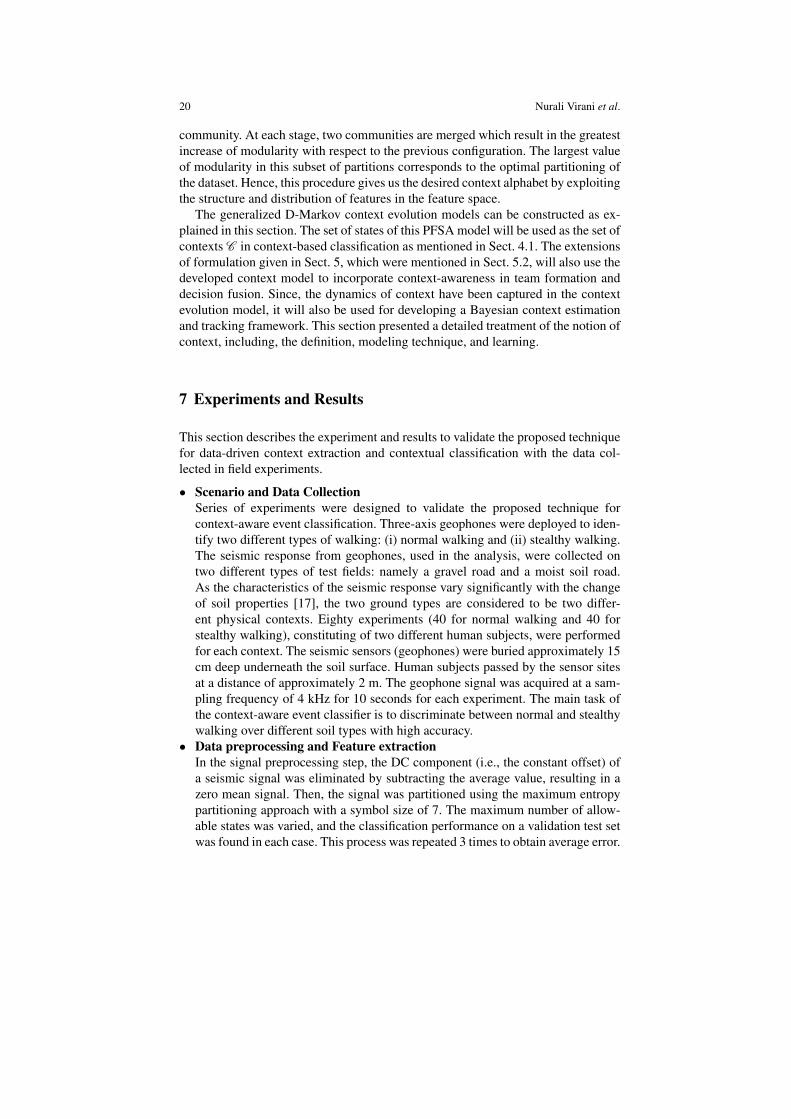
• Scenario and Data CollectionSeries of experiments were designed to validate the proposed technique forcontext-aware event classification. Three-axis geophones were deployed to iden-tify two different types of walking: (i) normal walking and (ii) stealthy walking.The seismic response from geophones, used in the analysis, were collected ontwo different types of test fields: namely a gravel road and a moist soil road.As the characteristics of the seismic response vary significantly with the changeof soil properties [17], the two ground types are considered to be two differ-ent physical contexts. Eighty experiments (40 for normal walking and 40 forstealthy walking), constituting of two different human subjects, were performedfor each context. The seismic sensors (geophones) were buried approximately 15cm deep underneath the soil surface. Human subjects passed by the sensor sitesat a distance of approximately 2 m. The geophone signal was acquired at a sam-pling frequency of 4 kHz for 10 seconds for each experiment. The main task ofthe context-aware event classifier is to discriminate between normal and stealthywalking over different soil types with high accuracy.

• Data preprocessing and Feature extractionIn the signal preprocessing step, the DC component (i.e., the constant offset) ofa seismic signal was eliminated by subtracting the average value, resulting in azero mean signal. Then, the signal was partitioned using the maximum entropypartitioning approach with a symbol size of 7. The maximum number of allow-able states was varied, and the classification performance on a validation test setwas found in each case. This process was repeated 3 times to obtain average error.


The number of states was then chosen to be 10, as it resulted in the best perfor-mance on the validation test set. After partitioning, symbolization was done andthe feature vectors were extracted by the method described in Sect. 2.1.2. Thesefeature vectors were later used for classification.

Fig. 5: Gravel Soil Fig. 6: Moist Soil

0 2 4 6 8 10−0.5

0

0.5

time

seis

mic

res

pons

e

normal walking

0 2 4 6 8 10−0.5

0

0.5

time

seis

mic

res

pons

e

stealthy walking

1 2 3 4 5 6 7 8 9 10 11 120

0.05

0.1

0.15

0.2

state index

prob

abili

ty

1 2 3 4 5 6 7 8 9 10 11 120

0.05

0.1

0.15

0.2

state index

prob

abili

ty

Fig. 7: Signals and Features

• Context Alphabet ConstructionThe entire dataset was randomly divided into training (60%) and testing (40%)sets ten times and the complete analysis was repeated for each combination oftraining and testing sets. Graph-theoretic techniques were then applied on thetraining data to get the context alphabet. The results were as follows:

1. Supervised Modeling: The features with the same event labels and same typeof soil were used to model the contextual observation densities. The k-nearestneighbor (k=6) algorithm was used as a nonparametric density modeling tech-nique. Symmetric KL divergence [16] was used as a metric of distance be-tween the observation densities. Two maximal cliques were obtained onefor each soil type; hence, the context alphabet size was 2. Note the human-understandable factors can be associated with machine-understandable con-text in supervised modeling. If a single maximal clique was obtained, it wouldimply that the features from those are similar and contextual classificationwould not significantly improve the performance.

2. Unsupervised Modeling: Figure 9 shows a modularity plot on a sampledataset of normal walking. The modularity of the graph configuration is high-est when there are two communities. Hence, observing the modularity plotgives the number of communities present, essentially yielding the context al-phabet. Since the ground truth context labels were available in the experiment,it was seen that the two communities detected by the algorithm actually cor-responded to the two different ground types.

• Classification PerformanceThe proposed analysis was performed for three different cases and the corre-sponding results are reported. The classifier used was a linear support vectormachine [9]. The following cases have been considered:


10 15 20 25 30 35

5

5.2

5.4

5.6

5.8

6

6.2

6.4

6.6

6.8

number of states

aver

age

num

ber

of m

iscl

assi

fied

sam

ples

Fig. 8: Selection of Number of States

0 10 20 30 40 50 60 70 80−0.1

−0.05

0

0.05

0.1

0.15

0.2

0.25

0.3

0.35

no of communities

Mod

ular

ity

Fig. 9: Modularity Score

1. No context knowledge: The training set had only the event labels. The knowl-edge that the data had been collected under two different physical contexts(Sect. 7) was not used in training; hence, just a single classifier was trained.This classifier was then used to classify the event of the test set. The contextknowledge was not available, yet the error was found to be 14.53±3.82% (Ta-ble. 1), which shows the robustness of the chosen feature extraction method.

2. Perfect context knowledge: The training set was labeled with the event andcontext symbols. A separate classifier was trained for each context symbolcorresponding to a ground type. A k-nearest neighbor classifier was trainedand used to assign the context symbol to the test set. The assigned symbol andthe feature were used to classify the event of this sample. Minimum classifi-cation error was obtained in this case (8±2.4% (Table. 1)), as expected.

3. With context identification: The training set had only the event labels. Bothunsupervised and supervised modeling yielded two context symbols. A k-nearest neighbor classifier was used to assign the context symbol to each testsample. The assigned symbol and the feature were then used to classify theevent of this sample. The average performance was 8.1%, almost same as case2, albeit with a larger standard deviation (2.81%). One reason for this couldbe that the extracted context might not always coincide with the ground truth,so the resulting classifiers might not be optimal under the true context.

Table 1: Experimental Results: Error Percentage in the three casesCase Mean Standard Deviation1 14.53 3.822 8 2.43 8.1 2.81

This experiment does not explicitly model or use context evolution, but a sim-ple D-Markov model with D = 1 and the probability of transition between differentstates are zero, which implies that the self-loop probability is one, represent thisscenario. This experiment shows that, if a sensor has been trained with data col-


lected from several sites, then during operation, it can first learn about the soil typeand use that knowledge for better target classification. Also, in this experiment, thebenefit of context-aware adaptation of decision boundaries is clearly visible as theperformance improves by choosing the appropriate classifier for the estimated con-text. Here, the features in different soil types were easily distinguishable, since, thismight not always be the case, a Bayesian context estimation and tracking frameworkwill also be developed.

8 Summary and Conclusions

The DDDAS formulation for the border surveillance problem, emphasizes the roleof context and context-awareness in target classification as well as measurementsystem adaptation. Techniques for understanding, modeling, and extracting contextfrom sensor data have been developed. This research is developing a DDDAS archi-tecture of context-aware multi-layered sensor network, which seems to be a viableand effective solution to the problem of persistent surveillance for border control.The current work will help improve target classification performance and selectionof optimal sensor suites in the settings of target classification. There are several av-enues for research, that need to be addressed for this problem: context evolutionlearning, novelty detection for new contexts, a framework to incorporate supervisedlearning feedback, game-theoretic interaction of multiple sensor teams competingfor shared resources, etc. These techniques need to be developed further and testedthoroughly, and finally put together into an on-line, low-power signal processing,and decentralized control implementation. The major contributions presented in thischapter are summarized as follows:

• A multi-layered sensor-net architecture for border surveillance was presented.• The importance of context was explained and a new mathematical definition for

data-driven and machine-understandable notion of context was formulated.• Two different context modeling techniques—namely, supervised and unsuper-

vised approaches—were developed for generating the context alphabet and wereused for developing context evolution models.

• The D-Markov machine, which is a powerful symbolic modeling tool for low-dimensional feature extraction from time series data, was succinctly explained.

• A technique for context-based classification, which was initially developed in [29],was presented briefly.

• The sensor network adaptation problem using the dynamic programming ap-proach was formulated and the solution approach with possible extensions ofthe work was also explained.

• An analysis with field data was presented, which showed significant improve-ment when the context (i.e., soil type) was estimated prior to event classification.


The modeling of context and context-aware adaptation presented in this chap-ter will be a good fit in many dynamic data-driven applications, including but notlimited to the following:

• Health monitoring, fault diagnosis, and prognosis in physical systems like auto-mobiles, battery systems, gas-turbine engines, etc.

• Target localization with several MOVINT sources, fused with HUMINT sourcesproviding extrinsic context.

• Indoor user localization with different fidelity and modality of data, such as WiFisignal strengths, ultrasonic chirp signals, cameras, and user inputs.

• Object recognition in large images by using a visual gist of the image as context.• Selecting contextually relevant channels for target classification and tracking in

a multi-modal or hyper-spectral imaging framework.

Studying the border surveillance problem over the years has shown that the inter-actions between environment and these sensor systems are very complex in practice,and that the DDDAS paradigm is crucial in overcoming this difficulty.

Acknowledgements The work reported in this chapter has been supported in part by U.S. AirForce Office of Scientific Research (AFOSR) under Grant No. FA9550-12-1-0270 and by U.S.Army Research Office (ARO) under Grant No. W911NF-13-1-0461. Any opinions, findings, andconclusions or recommendations expressed in this paper are those of the authors and do not neces-sarily reflect the views of the sponsoring agencies.

References

[1] Adenis P, Mukherjee K, Ray A (2011) State splitting and state merging in probabilistic finitestate automata. Proc American Control Conference, San Francisco, CA, USA pp 5145–5150

[2] Akkoyunlu EA (1973) The enumeration of maximal cliques of large graphs. SIAM Journalon Computing 2:1–6

[3] Bahrampour S, Ray A, Sarkar S, Damarla T, Nasrabadi NM (2013) Performance comparisonof feature extraction algorithms for target detection and classification. Pattern RecognitionLetters 34(16):2126–2134

[4] Bland RE (2006) Acoustic and seismic signal processing for footstep detection. Master’sthesis, Massachusetts Institute of Technology, Dept. of Electrical Engineering and ComputerScience

[5] Blasch E, Plano S (2005) Dfig level 5 (user refinement) issues supporting situational assess-ment reasoning. In: 8th International Conference on Information Fusion, IEEE, vol 1, ppxxxv–xliii

[6] Blasch E, Herrero J, Snidaro L, Llinas J, Seetharaman G, Palaniappan K (2013) Overview ofcontextual tracking approaches in information fusion. In: Proceedings of SPIE

[7] Bron C, Kerbosch J (1973) Algorithm 457: Finding all cliques of an undirected graph. Com-muncations of ACM 16(9):575–577

[8] Cazals F, Karande C (2008) A note on the problem of reporting maximal cliques. TheoreticalComputer Science 407(1):564–568

[9] Christopher B (1998) A tutorial on support vector machines for pattern recognition. DataMining and Knowledge Discovery 2:121–167


[10] Dey A, Abowd G (1999) Towards a better understanding of context and context awareness.In: HUC’99: Proceedings of the 1st International Symposium on Handheld and Ubiquitouscomputing, Springer-Verlag, pp 304–307

[11] Elnahrawy E, Nath B (2004) Context-aware sensors. In: EWSN[12] Fortunato S (2010) Community detection in graphs. Physics Reports 486:75–174[13] Girvan M, Newman MEJ (2002) Community structure in social and biological networks.

Proceedings of the National Academy of Sciences of the United States of America 99:7821–7826

[14] Iyengar SG, Varshney PK, Damarla T (2007) On the detection of footsteps based on acousticand seismic sensing. In: Forty-First Asilomar Conference on Signals, Systems and ComputersACSSC, pp 2248–2252

[15] Jin X, Sarkar S, Ray A, Gupta S, Damarla T (2012) Target detection and classification usingseismic and PIR sensors. IEEE Sensors Journal 12(6):1709–1718

[16] Kullback S, Leibler RA (1951) On information and sufficiency. The Annals of MathematicalStatistics 22(1):79–86

[17] McKenna JR, McKenna MH (2006) Effects of local meteorological variability on surface andsubsurface seismic-acoustic signals. Tech. rep., DTIC Document

[18] Mukhopadhyay A, Chaudhari RR, Paul T, Sen S, Ray A (2013) Lean blow-out prediction ingas turbine combustors using symbolic time series analysis. Journal of Propulsion and Powerpp 1–11

[19] Newman M (2003) Fast algorithm for detecting community structure in networks. PhysicalReview E 69

[20] Olivaa A, Torralba A (2007) The role of context in object recognition. Trends in CognitiveSciences pp 520–527

[21] Phoha S, Virani N, Chattopadhyay P, Sarkar S, Smith B, Ray A (2014) Context-aware dy-namic data-driven pattern classification. In: International Conference on Computational Sci-ence (ICCS) (accepted)

[22] Ray A (2004) Symbolic dynamic analysis of complex systems for anomaly detection. SignalProcessing 84(7):1115–1130

[23] Sarkar S, Sarkar S, Mukherjee K, Ray A, Srivastav A (2012) Multi-sensor information fusionfor fault detection in aircraft gas turbine engines. Proceedings of the Institution of MechanicalEngineers, Part G: Journal of Aerospace Engineering

[24] Sarkar S, Mukherjee K, Sarkar S, Ray A (2013) Symbolic dynamic analysis of transient timeseries for fault detection in gas turbine engines. Journal of Dynamic Systems, Measurement,and Control 135:14,506–11

[25] Sarkar S, Virani N, Yasar M, Ray A, Sarkar S (2013) Spatiotemporal information fusionfor fault detection in shipboard auxiliary systems. In: American Control Conference (ACC),2013, IEEE, pp 3846–3851

[26] Shi X, Linga H, Blasch E, Hu W (2012) Context-driven moving vehicle detection in widearea motion imagery. In: ICPR, pp 2512–2515

[27] Sonti S, Keller E, Horn J, Ray A (2014) Stability monitoring of rotorcraft systems: Adynamic data-driven approach. Journal of Dynamic Systems, Measurement, and Control136(2):024,505

[28] Tomita E, Tanaka A, Takahashi H (2006) The worst-case time complexity for generating allmaximal cliques and computational experiments. Theoretical Computer Science 363(1):28–42

[29] Virani N, Marcks S, Sarkar S, Mukherjee K, Ray A, Phoha S (2013) Dynamic data-driven sensor array fusion for target detection and classification. Procedia Computer Science18:2046–2055

[30] Wilson DK, Marlin D, Mackay S (2007) Acoustic/seismic signal propagation and sensorperformance modeling. In: SPIE, vol 6562

a context-aware multi-layered sensor network for border ...€¦ · a context-aware multi-layered...

Documents