a critical evaluation of the predictive capabilities of...

A Critical Evaluation of the Predictive Capabilities of

Various Advanced Micromechanics Models

Wenbin Yu∗

Utah State University, Logan, Utah 84322-4130

Todd O. Williams†

Los Alamos National Laboratory, Los Alamos, New Mexico 87545

Brett A. Bednarcyk‡

Ohio Aerospace Institute, Cleveland, OH 44142

Jacob Aboudi§

Tel-Aviv University, Ramat-Aviv, Israel

and

Tian Tang¶

Utah State University, Logan, Utah 84322-4130

The focus of this work is to critically evaluate the predictive capabilities of severaladvanced micromechanics models, including GMC, HFGMC, ECM, and VAMUCH. Thecomparison concentrates primarily on predictions for the effective elastic properties andlocal stress fields based on micromechanics approaches for various types of composite sys-tems. Both exact analytical solutions and finite element simulations will be utilized inthe comparison to assess the accuracy of the different models. It is found that for somemicrostructures, most of the compared models provide similar and reliable predictions foreffective properties. For an accurate prediction for local stress distributions, HFGMC andVAMUCH significantly outperform GMC, which provides only average local fields. A verychallenging X shape microstructure is also proposed in this paper which pushes all themicromechanics models to their limits. This case clearly discloses the fallacy about mi-cromechanics that every model “works” as far as effective properties concerned. Such anassessment can help engineers choose the appropriate micromechanics model for compositesthey are dealing with in their applications.

Introduction

As structural applications become more demanding it is becoming increasingly important that the fun-damental response mechanisms controlling both the microscopic and macroscopic behavior of structuralmaterials be well understood. Properly quantified in a material model such understanding can be used toimprove structural designs, make more accurate estimates of a given structure’s capabilities, or engineer amaterial’s microstructure in order to enhance desirable performance characteristics.

The fundamental response mechanisms in all heterogeneous materials are driven by the localization pro-cesses induced by the presence of the heterogeneities (the microstructures) that exist in these materials.Micromechanical theories are particularly well suited to modeling localization processes and how they in-fluence the micro- and macroscopic material behavior since these theories predict the multiscale material

∗Assistant Professor, Department of Mechanical and Aerospace Engineering. Senior Member, AIAA; Member, ASME andAHS.

†Technical Staff Member, Theoretical Division, T-3.‡Senior Scientist, Member, AIAA.§Professor, Department of Solid Mechanics, Materials and Structures¶Graduate Research Assistant, Department of Mechanical and Aerospace Engineering. Student Member, AIAA.

1 of 17

American Institute of Aeronautics and Astronautics

48th AIAA/ASME/ASCE/AHS/ASC Structures, Structural Dynamics, and Materials Con23-26 April 2007, Honolulu, Hawaii

AIAA 2007-2084

This material is declared a work of the U.S. Government and is not subject to copyright protection in the United States.

response based directly on a knowledge of the behavior of the individual component materials and of theheterogeneous microstructure.

There are a number of different types of homogenization tools available. The simplest such models,1,2

which are based on strength of materials assumptions, can only be considered to give very rough estimatesfor a material’s response characteristics. Mean field theories, such as the Mori-Tanaka theory3,4 can providereasonable estimates for a material’s bulk elastic response but typically fail to provide good estimates for thelocal responses and the history-dependent responses of the material. In order to correctly predict the localand bulk response characteristics in the elastic and inelastic domains it is necessary to utilize micromechanicaltheories that consider both the average fields within phases as well as the fluctuating fields within the phases.5

A set of relatively simple micromechanical models that have attempted to develop such capabilities are theso-call “Method of Cells” (MOC)6 and the “Generalized Method of Cells” (GMC).7,8 These approaches arebased on the use of average strain and stress fields within discrete subvolumes of the microstructure. A reviewof some of the published work using these models is given in Ref. 9. One shortcoming of the MOC/GMCmodels is the lack of coupling between the local shearing and normal responses for composites composed ofphases with at least orthotropic symmetry. This lack of coupling has significant implications for predictingthe history-dependent behavior of such materials. In order to overcome this lack of coupling in the local fieldsit is necessary to utilize theories with more accurate representations of the local fields. There are a numberof such theories currently available. Two very different approaches that have been developed in an attemptto directly address the lack of coupling in the MOC/GMC set of models are the so-called “High FidelityGeneralized Method of Cells” (HFGMC) model10 and the so-called “Elasticity-based Cell Model”.5,11,12

Obviously, various other models that exhibit (potentially) accurate representations of the microfields inthe composite exist which have no connection to the original MOC/GMC methodologies. Examples ofsuch theories are Green’s function based analyses13 and asymptotic homogenization approaches.14 A recentlydeveloped variant of the asymptotic homogenization approach is the Variational Asymptotic Method for UnitCell Homogenization (VAMUCH).15–17 In contrast to conventional asymptotic methods, VAMUCH carriesout an asymptotic analysis of the variational statement, synthesizing the merits of both variational methodsand asymptotic methods. Finally, there are a number of purely numerical approaches, such as finite elementanalyses,18,19 and particle-in-cell methods,20 that have been used to model the micromechanical response ofheterogeneous materials.

Obviously, significant effort has been expended to develop a number of approaches that can be usedto consider the micromechanical responses of composite systems. However, there has been relatively littlework done that compares the predictive capabilities of different approaches. One such study, carried out byLissenden and Herakovich,21 considered the ability of various simplified micromechanical theories to predictthe bulk elastic properties of continuous fiber composites. However, in today’s environment of advancedapplications it is no longer sufficient to consider only the predictions for the bulk characteristics. It is nownecessary to consider the predictive capabilities for the local fields within the material system.

The focus of the current work is the comparison of the predictive capabilities of several advanced mi-cromechanical theories; the GMC theory, the HFGMC theory, the ECM theory, and VAMUCH, with eachother as well as with established analytical solutions and finite element predictions. The work will considerboth the local and global responses. Since accurate predictions for the elastic fields within the composite area necessary prerequisite for accurately predicting the history-dependent behavior of heterogeneous materialsthe current comparisons focus on the elastic predictions.

The Generalized Method of Cells (GMC)

The starting point for the GMC theory is the discretization of the periodic material microstructure intorectangular (for the two-dimensional (2D) theory) or rectilinear parallelepiped (for the three-dimensional(3D) theory) subregions; see Fig. 1. Each of these subregions is termed a subcell. The displacement fieldwithin each subcell is modeled using the representation (for 3D microstructures)

u(α,β,γ)i = Ψ(α,β,γ)

i x1 + Γ(α,β,γ)i x2 + Ω(α,β,γ)

i x3 (1)

This displacement field representation results in uniform strains within each subcell (although the strains indifferent subcells are typically different).

Satisfaction of the displacement continuity conditions between subcells as well as between repeatingmaterial volumes, either unit cells (UC) or representative volume elements (RVEs), gives the following set

2 of 17


Figure 1. The discretized repeating volume for a particulate composite used by the original GMC model, theHFGMC theory, and the ECM.

of governing equations

Nα∑α=1

dαΨ(α,β,γ)1 =

(Nα∑α=1

dα

)ε11

Nβ∑

β=1

hβΓ(α,β,γ)2 =

Nβ∑

β=1

hβ

ε22

Nγ∑γ=1

lγΩ(α,β,γ)3 =

Nγ∑γ=1

lγ

ε33

Nβ∑

β=1

Nγ∑γ

hβlγε(α,β,γ)23 =

Nβ∑

β=1

Nγ∑γ

hβlγ

ε23

Nα∑α=1

Nγ∑γ

dαlγε(α,β,γ)13 =

Nα∑α=1

Nγ∑γ

dαlγ

ε13

Nα∑α=1

Nβ∑

β

dαhβε(α,β,γ)12 =

Nα∑α=1

Nβ∑

β

dαhβ

ε12 (2)

3 of 17


where εij are the applied average strain field and where

ε(α,β,γ)23 =

(Ω(α,β,γ)

2 + Γ(α,β,γ)3

)/2

ε(α,β,γ)13 =

(Ω(α,β,γ)

1 + Ψ(α,β,γ)3

)/2

ε(α,β,γ)12 =

(Ψ(α,β,γ)

2 + Γ(α,β,γ)1

)/2 (3)

Satisfaction of the traction continuity conditions in an average sense between subcells as well as betweenrepeating material volumes gives the following governing relations

σ(α,β,γ)11 = σ

(α+1,β,γ)11 for α = 1, .., Nα − 1, β = 1, .., Nβ , γ = 1, .., Nγ

σ(α,β,γ)22 = σ

(α,β+1,γ)22 for α = 1, .., Nα, β = 1, .., Nβ − 1, γ = 1, .., Nγ

σ(α,β,γ)33 = σ

(α,β,γ+1)33 for α = 1, .., Nα, β = 1, .., Nβ , γ = 1, .., Nγ − 1

σ(α,β,γ)23 = σ

(α,β,γ+1)23 for α = 1, .., Nα, β = 1, .., Nβ − 1, γ = 1, .., Nγ

σ(α,β,γ)23 = σ

(α,β+1,γ)23 for α = 1, .., Nα, β = Nβ , γ = 1, ..., Nγ − 1

σ(α,β,γ)13 = σ

(α,β,γ+1)13 for α = 1, .., Nα − 1, β = 1, .., Nβ , γ = 1, .., Nγ

σ(α,β,γ)13 = σ

(α+1,β,γ)13 for α = Nα − 1, β = 1, .., Nβ , γ = 1, ..., Nγ − 1

σ(α,β,γ)12 = σ

(α,β+1,γ)12 for α = 1, .., Nα − 1, β = 1, .., Nβ , γ = 1, .., Nγ

σ(α,β,γ)12 = σ

(α+1,β,γ)12 for α = Nα, β = 1, ..., Nβ − 1, γ = 1, .., Nγ (4)

The above system of governing equations can be cast in the following matrix form

Aεs − D(εIs + εT

s

)= Kε (5)

Solving Eqn. (5) for the subcell strains εs yields

εs = Aε + D(εIs + εT

s

)(6)

where A and D are the mechanical and eigenstrain concentration tensors, respectively.The bulk constitutive relations for the composite

σ = B∗ (ε− εI − εT

)(7)

are obtained by substituting Eqn. (6) into the average stress theorem. Explicit expressions for the terms B∗,εI , and εT are give in Ref. 8.

There are a couple of characteristics in the GMC theory that should be kept in mind. First, as mentionedpreviously there is no geometrically induced coupling between the local normal and shearing effects. Addi-tionally, there is no geometrically induced coupling between the local shearing effects. Since the stresses ineach subcell are spatially uniform within the subcell every subcell along a given row of subcells (in any ofthe directions) experiences the same stress along that direction. Furthermore, the behavior along the row istypically dominated by the most compliant material in the row. These characteristics of the GMC approachwere utilized in Refs. 22 and 23 to reformulate the 2D and 3D versions of GMC, respectively, in order tomaximize the computational efficiency of the method (i.e., minimize the number of unknown variables). Forfull details of the GMC formulation for see Ref. 7 for 2D UCs and Ref. 8 for 3D UCs.

The High-Fidelity Generalized Method of Cells Theory (HFGMC)

The version of HFGMC that is described herein is designated for the prediction of the effective ther-moinelastic behavior of composites with discontinuous fibers (i.e., short-fiber composites). This three-dimensional, triply periodic theory has been fully described in Ref. 10 in the case of linear electro-magneto-thermo-elastic materials. Thus, thermoelastic phases can by obtained as a special case. The inclusion ofinelastic effects in the phases follows the analysis that has been presented in Ref. 24 in the two-dimensionalcase of continuous fibers. This micromechanical model is briefly outlined in the following.

4 of 17


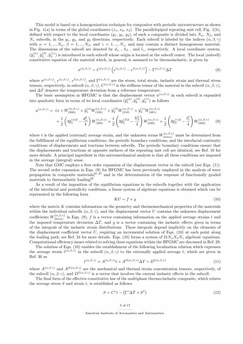
This model is based on a homogenization technique for composites with periodic microstructure as shownin Fig. 1(a) in terms of the global coordinates (x1, x2, x3). The parallelepiped repeating unit cell, Fig. 1(b),defined with respect to the local coordinates (y1, y2, y3), of such a composite is divided into Nα, Nβ , andNγ subcells, in the y1, y2, and y3 directions, respectively. Each subcell is labeled by the indices (α, β, γ)with α = 1, ..., Nα, β = 1, ..., Nβ , and γ = 1, ..., Nγ , and may contain a distinct homogeneous material.The dimensions of the subcell are denoted by dα , hβ , and lγ , respectively. A local coordinate system,(y(α)

1 , y(β)2 , y

(γ)3 ) is introduced in each subcell whose origin is located at the subcell center. The local (subcell)

constitutive equation of the material which, in general, is assumed to be thermoinelastic, is given by

σ(α,β,γ) = C(α,β,γ)(ε(α,β,γ) − εI(α,β,γ)

)− Γ(α,β,γ)∆T (8)

where σ(α,β,γ), ε(α,β,γ), εI(α,β,γ), and Γ(α,β,γ) are the stress, total strain, inelastic strain and thermal stresstensors, respectively, in subcell (α, β, γ), C(α,β,γ) is the stiffness tensor of the material in the subcell (α, β, γ),and ∆T denotes the temperature deviation from a reference temperature.

The basic assumption in HFGMC is that the displacement vector u(α,β,γ) in each subcell is expandedinto quadratic form in terms of its local coordinates (y(α)

1 , y(β)2 , y

(γ)3 ) as follows

u(α,β,γ) = εx + W(α,β,γ)(000) + y

(α)1 W

(α,β,γ)(100) + y

(β)2 W

(α,β,γ)(010) + y

(γ)3 W

(α,β,γ)(001)

+12

(3y

(α)21 − d2

α

4

)W

(α,β,γ)(200) +

12

(3y

(β)22 − h2

β

4

)W

(α,β,γ)(020) +

12

(3y

(γ)23 − l2γ

4

)W

(α,β,γ)(002) (9)

where ε is the applied (external) average strain, and the unknown terms W(α,β,γ)(kmn) must be determined from

the fulfillment of the equilibrium conditions, the periodic boundary conditions, and the interfacial continuityconditions of displacements and tractions between subcells. The periodic boundary conditions ensure thatthe displacements and tractions at opposite surfaces of the repeating unit cell are identical, see Ref. 10 formore details. A principal ingredient in this micromechanical analysis is that all these conditions are imposedin the average (integral) sense.

Note that GMC employs a first order expansion of the displacement vector in the subcell (see Eqn. (1)).The second order expansion in Eqn. (9) for HFGMC has been previously employed in the analysis of wavepropagation in composite materials,25–27 and in the determination of the response of functionally gradedmaterials to thermoelastic loading.28

As a result of the imposition of the equilibrium equations in the subcells together with the applicationof the interfacial and periodicity conditions, a linear system of algebraic equations is obtained which can berepresented in the following form

KU = f + g (10)

where the matrix K contains information on the geometry and thermomechanical properties of the materialswithin the individual subcells (α, β, γ), and the displacement vector U contains the unknown displacementcoefficients W

(α,β,γ)(kmn) in Eqn. (9), f is a vector containing information on the applied average strains ε and

the imposed temperature deviation ∆T , and g is a vector containing the inelastic effects given in termsof the integrals of the inelastic strain distributions. These integrals depend implicitly on the elements ofthe displacement coefficient vector U , requiring an incremental solution of Eqn. (10) at each point alongthe loading path, see Ref. 24 for more details. Eqn. (10) forms a system of 21NαNβNγ algebraic equations.Computational efficiency issues related to solving these equations within the HFGMC are discussed in Ref. 29.

The solution of Eqn. (10) enables the establishment of the following localization relation which expressesthe average strain ε(α,β,γ) in the subcell (α, β, γ) to the externally applied average ε, which are given inRef. 30 as

ε(α,β,γ) = A(α,β,γ)ε + Ath(α,β,γ)∆T + DI(α,β,γ) (11)

where A(α,β,γ) and Ath(α,β,γ) are the mechanical and thermal strain concentration tensors, respectively, ofthe subcell (α, β, γ), and DI(α,β,γ) is a vector that involves the current inelastic effects in the subcell.

The final form of the effective constitutive law of the multiphase thermo-inelastic composite, which relatesthe average stress σ and strain ε, is established as follows:

σ = C∗ε− (Γ∗∆T + σI

)(12)

5 of 17


In this equation C∗ is the effective stiffness tensor and Γ∗ is the effective thermal stress tensor of thecomposite, and σI is the global inelastic stress tensor. All of these global quantities can be expressed in aclosed-form manner in terms of the mechanical and thermal concentration tensors which appear in Eqn. (11)together with the inelastic term DI(α,β,γ), which are given in Ref. 30 as follows

C∗ =1

DHL

Nα∑α=1

Nβ∑

β=1

Nγ∑γ=1

dαhβlγC(α,β,γ)A(α,β,γ)

Γ∗ = − 1DHL

Nα∑α=1

Nβ∑

β=1

Nγ∑γ=1

dαhβlγ

(C(α,β,γ)Ath(α,β,γ) − Γ(α,β,γ)

)

σI = − 1DHL

Nα∑α=1

Nβ∑

β=1

Nγ∑γ=1

dαhβlγ

(C(α,β,γ)DI(α,β,γ) −R

(α,β,γ)(000)

)(13)

where R(α,β,γ)(000) is an expression that represents the integral of the inelastic strain distributions.

Based on the generalized method of cells family of models, the NASA Glenn Research Center developeda micromechanics computer code, referred to as MAC/GMC, that has many user-friendly features andsignificant flexibility for the analysis of continuous, discontinuous, and woven polymer, ceramic, and metalmatrix composites with phases that can be represented by arbitrary elastic, viscoelastic, and/or viscoplasticconstitutive models. The most recent version of a user guide to this code (version 4) which has been presentedby Bednarcyk and Arnold31 incorporates HFGMC, together with additional material models including smartmaterials (electromagnetic and shape memory alloys) and yield surface prediction of metal matrix composites.

The Elasticity-Based Cell Model (ECM)

The Elasticity-Based Cell Model (ECM)5,11,12 starts with the same type of microstructural discretizationas used by the original GMC theory, Fig. 1. The displacement field within each subcell is given in terms ofan infinite series

u(α1,α2,α3)i

(x, y

)= εijxj + P

(α1,α2,α3)(o1,o2,o3)

(y)V

(α1,α2,α3)i(o1,o2,o3)

(14)

where the εij are the components of the bulk strain field, the xj are the macroscopic coordinate components,P

(α1,α2,α3)(o1,o2,o3)

(y)

= p(α1)(o1)

(y1)p(α2)(o2)

(y2)p(α3)(o3)

(y3) and the p(oi) are orthogonal polynomial terms of order oi in theyi (the local coordinate) directions in the subcells. The corresponding subcell strain and stress fields aregiven by

ε(α1,α2,α3)ij = P

(α1,α2,α3)(0,0,0) εij + P

(α1,α2,α3)(o1,o2,o3)

µ(α1,α2,α3)ij(o1,o2,o3)

σ(α1,α2,α3)ij = P

(α1,α2,α3)(o1,o2,o3)

σ(α1,α2,α3)ij(o1,o2,o3)

(15)

The µ(α1,α2,α3)ij(o1,o2,o3)

represent the fluctuating strain effects. Summation on repeated order indices, oi, is assumed.Making use of the orthogonality properties of the expansions functions the equilibrium equations are

satisfied byσ

(α1,α2,α3)1j(o′1,o2,o3)

a(α1)(o′1,o1)

+ σ(α1,α2,α3)2j(o1,o′2,o3)

a(α2)(o′2,o2)

+ σ(α1,α2,α3)3j(o1,o2,o′3)

a(α1)(o′3,o3)

= 0 (16)

which results in pointwise satisfaction of the equilibrium conditions.Imposing traction continuity in terms of the different expansion orders within the subcell surfaces (both

between subcells within a repeating volume as well as between repeating volumes) gives

σ(α1,α2,α3)1i(o1,o2,o3)

p(α1)o1

(δ(α1)(1)

)= σ

(α1,α2,α3)1i(o1,o2,o3)

p(α1)o1

(−δ

(α1)(1)

)

σ(α1,α2,α3)2i(o1,o2,o3)

p(α2)o2

(δ(α2)(2)

)= σ

(α1,α2,α3)2i(o1,o2,o3)

p(α2)o2

(−δ

(α2)(2)

)

σ(α1,α2,α3)3i(o1,o2,o3)

p(α3)o3

(δ(α3)(3)

)= σ

(α1,α2,α3)3i(o1,o2,o3)

p(α3)o3

(−δ

(α3)(3)

)(17)

6 of 17


where δ(αi)(i) = dαi

(i)/2. As was the case for the equilibrium conditions the above equations represent pointwisesatisfaction of the interfacial traction continuity constraints.

Following similar procedures to those used to obtain the traction continuity equations, the displacementcontinuity conditions at the different interfaces are seen to be satisfied by

p(α1)o1

(δ(α1)(1)

)V

(α1,α2,α3)i(o1,o2,o3)

= p(α1)o1

(−δ

(α1)(1)

)V

(α1,α2,α3)i(o1,o2,o3)

p(α2)o2

(δ(α2)(2)

)V

(α1,α2,α3)i(o1,o2,o3)

= p(α2)o2

(−δ

(α2)(2)

)V

(α1,α2,α3)i(o1,o2,o3)

p(α3)o3

(δ(α3)(3)

)V

(α1,α2,α3)i(o1,o2,o3)

= p(α3)o3

(−δ

(α3)(3)

)V

(α1,α2,α3)i(o1,o2,o3)

(18)

for αi = 1, .., Ni. The above forms of the interfacial displacement conditions result in pointwise satisfactionof these constraints.

Once a set of constitutive relations for the phases has been specified the above set of governing equationscan be directly expressed in terms of the fundamental kinematic unknowns, V

(α1,α2,α3)i(o1,o2,o3)

. A sufficiently generalform for the history-dependent constitutive relations relating the subcell stress and strain fields is given by

σij = Lijklεkl + λij (19)

where the Lijkl are the material stiffness components and the λij are the eigenstresses which represent theevolving history-dependent response of a material. The forms of the governing equations based on the aboveconstitutive form are not given here for conciseness (see Ref. [5] for these details).

The above system of governing equations can be cast in the form

BV = Aε + Fλ (20)

which in turn can be solved for the concentration tensors to give

µ(α1,α2,α3) = A(α1,α2,α3)ε + F (α1,α2,α3|β1,β2,β3)λ(β1,β2,β3) (21)

For the full details of the ECM formulation (both infinite series and general truncated expansions) see Ref. [5].The formulations for specialized microstructures are given in Refs. [11, 12].

The Variational Asymptotic Method for Unit Cell Homogenization (VAMUCH)

Recently, a new micromechanics model, the Variational Ssymptotic Method for Unit Cell Homogenization(VAMUCH),15–17 has been developed by invoking three assumptions: 1) size of the microstructure is muchsmaller than the macroscopic size of the material; 2) exact solutions of the field variables have volumeaverages over the UC; 3) effective material properties are independent of macroscopic geometry, boundaryand loading conditions of the structure.

The derivation of VAMUCH starts from a variational statement of the heterogenous continuum. Tak-ing advantage of the smallness of the microstructure, one can formulate the homogenization problem as aconstrained minimization problem posed over a single UC by carrying out an asymptotic analysis of thevariational statement. The final theory of VAMUCH for homogenizing elastic materials can be obtained byminimizing

ΠΩ =1

2Ω

∫

Ω

Cijkl

[εij + χ(i|j)

] [εkl + χ(k|l)

]dΩ (22)

subject to the following constraints

χi(x; d1/2, y2, y3) = χi(x;−d1/2, y2, y3) (23)χi(x; y1, d2/2, y3) = χi(x; y1,−d2/2, y3) (24)χi(x; y1, y2, d3/2) = χi(x; y1, y2,−d3/2) (25)〈χi〉 = 0 (26)

where Eqs. (23)-(25) are the well-known periodic boundary conditions and Eqn. (26) helps uniquely determinethe fluctuation functions χi. Following the regular steps of calculus of variations, one can easily show thatthe Euler-Lagrange equations corresponding to this constrained minimization problem are the same as theMathematical Homogenization Theories (MHT).15 Although VAMUCH can achieve the same accuracy ofMHT, VAMUCH is different from MHT in at least the following three aspects:

7 of 17


• The periodic boundary conditions are derived in VAMUCH, while they are assumed a priori in MHT.

• The fluctuation functions are determined uniquely in VAMUCH due to Eq. (26), while they can onlybe determined up to a constant in MHT.

• VAMUCH has an inherent variational nature which is convenient for numerical implementation, whilevirtual quantities should be carefully chosen to make MHT variational.32

This constrained minimization problem can be solved analytically for very simple cases such as binarycomposites.15 For general cases we need to turn to computational techniques for numerical solutions. SinceVAMUCH theory is variational, the finite element method is a natural choice as a method to solve thisproblem. The details of finite element implementation are given in Ref. [16]. As the result, a companioncode VAMUCH has been developed as a general-purpose micromechanical analysis code. Although VAMUCHhas all the versatility of the finite element method, it is by no means the traditional displacement-base finiteelement analysis. The code VAMUCH has the following distinctive features:

• No external load is necessary to perform the simulation and the complete set of material propertiescan be predicted within one analysis.

• The fluctuation functions and local displacements can be determined uniquely;

• The effective material properties and recovered local fields are calculated directly with the same accu-racy of the fluctuation functions. No postprocessing type calculations such as averaging stresses andaveraging strains are needed

• The dimensionality of the problem is determined by that of the periodicity of the UC. A complete 6×6effective material matrix can be obtained even for a 1D unit cell.

For details of VAMUCH theory and implementation, please refer to Refs. [15–17].

Case Studies

These micromechanics models will be used to predict the bulk and local elastic responses of various typesof fiber reinforced composites. The resulting predictions will be compared to assess the accuracy with whichthe different models are capable of predicting the local fields as well as the effective bulk properties of differentcomposite systems. For the purpose of comparison, we also use a finite element based micromechanicsapproach (which is denoted as FEM) proposed by Sun and Vaidya.18 This method performs the conventionalstress analysis of a representative volume element by applying periodic and symmetric boundary conditions.In this work, we used ANSYS to perform all the needed finite element analysis. Using this approach, onlythe transverse shear moduli G23 can be calculated using 2D analysis, and all the other effective propertiesare calculated using 3D analysis. However, all the other micromechanics models reviewed in the previoussection only require a 2D analysis for fiber reinforced composites.

A. Case 1: Eshelby problem

The first case is the Eshelby problem33 which deals with an isotropic circular fiber embedded in an infiniteisotropic matrix subjected to the uniform far-field stress σ∞22 . It is a plane strain elasticity problem and canbe solved exactly. Although this is not a micromechanics problem because no repeating UCs can be identifiedin the material, we can consider a material with repeating UCs which have sufficiently small fiber volumefraction (we choose 1% for this example) so that the interaction effects due to the presence of adjacent cellsare negligible. Except for this restriction, the exact solution provides an excellent benchmark for validationof the accuracy of the local fields predicted by different micromechanics models.

For calculation, we choose the fiber to be boron with Young’s modulus E = 400.0 GPa and Poisson’sratio ν = 0.20, the matrix to be epoxy with Young’s modulus E = 3.50 GPa and Poisson’s ratio ν = 0.35.The choice of these materials produces a high elastic moduli mismatch and thus a significant disturbancein the stress field along the interface between fiber and matrix. To obtain the stress distribution within theUC using micromechanics approaches, we need to calculate the effective properties first, which are listed inTable 1. It can be observed that except for GMC, which slightly under predicts the moduli (E22, G12, G23)

8 of 17


Table 1. Effective properties of boron/epoxy composites for Eshelby problem

Models E11 (MPa) E22 (MPa) G12 (MPa) G23 (MPa) ν12 ν23

GMC 7465 3785 1311 1309 0.3484 0.4435HFGMC 7466 3801 1322 1317 0.3481 0.4424

ECM (5th order) 7466 3793 1315 1313 0.3482 0.4431VAMUCH 7466 3801 1322 1317 0.3481 0.4424

FEM 7466 3801 1322 1317 0.3481 0.4424

S22 contour plot of Eshelby solution: Ansys results

2y

3y

S22 contour plot of Eshelby solution: Ansys results

2y

3y

Figure 2. Contour plot of σ22 (MPa)

S23 contour : Ansys results

2y

3y

S23 contour : Ansys results

2y

3y

Figure 3. Contour plot of σ23 (MPa)

9 of 17


and over predicts the Poisson’s ratios, all the other approaches obtain the same results up to the fourthsignificant figure.

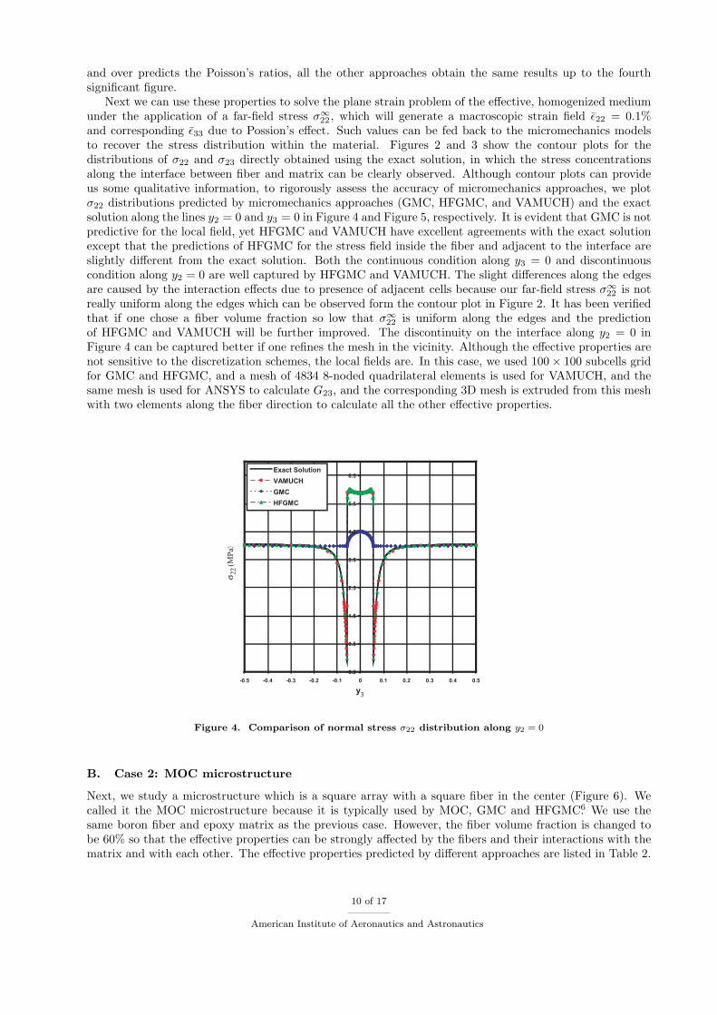
Next we can use these properties to solve the plane strain problem of the effective, homogenized mediumunder the application of a far-field stress σ∞22 , which will generate a macroscopic strain field ε22 = 0.1%and corresponding ε33 due to Possion’s effect. Such values can be fed back to the micromechanics modelsto recover the stress distribution within the material. Figures 2 and 3 show the contour plots for thedistributions of σ22 and σ23 directly obtained using the exact solution, in which the stress concentrationsalong the interface between fiber and matrix can be clearly observed. Although contour plots can provideus some qualitative information, to rigorously assess the accuracy of micromechanics approaches, we plotσ22 distributions predicted by micromechanics approaches (GMC, HFGMC, and VAMUCH) and the exactsolution along the lines y2 = 0 and y3 = 0 in Figure 4 and Figure 5, respectively. It is evident that GMC is notpredictive for the local field, yet HFGMC and VAMUCH have excellent agreements with the exact solutionexcept that the predictions of HFGMC for the stress field inside the fiber and adjacent to the interface areslightly different from the exact solution. Both the continuous condition along y3 = 0 and discontinuouscondition along y2 = 0 are well captured by HFGMC and VAMUCH. The slight differences along the edgesare caused by the interaction effects due to presence of adjacent cells because our far-field stress σ∞22 is notreally uniform along the edges which can be observed form the contour plot in Figure 2. It has been verifiedthat if one chose a fiber volume fraction so low that σ∞22 is uniform along the edges and the predictionof HFGMC and VAMUCH will be further improved. The discontinuity on the interface along y2 = 0 inFigure 4 can be captured better if one refines the mesh in the vicinity. Although the effective properties arenot sensitive to the discretization schemes, the local fields are. In this case, we used 100× 100 subcells gridfor GMC and HFGMC, and a mesh of 4834 8-noded quadrilateral elements is used for VAMUCH, and thesame mesh is used for ANSYS to calculate G23, and the corresponding 3D mesh is extruded from this meshwith two elements along the fiber direction to calculate all the other effective properties.

22

-0.5

0.5

1.5

2.5

3.5

4.5

5.5

6.5

-0.5 -0.4 -0.3 -0.2 -0.1 0 0.1 0.2 0.3 0.4 0.5

Exact Solution

VAMUCH

GMC

HFGMC

y23

Figure 4. Comparison of normal stress σ22 distribution along y2 = 0

B. Case 2: MOC microstructure

Next, we study a microstructure which is a square array with a square fiber in the center (Figure 6). Wecalled it the MOC microstructure because it is typically used by MOC, GMC and HFGMC.6 We use thesame boron fiber and epoxy matrix as the previous case. However, the fiber volume fraction is changed tobe 60% so that the effective properties can be strongly affected by the fibers and their interactions with thematrix and with each other. The effective properties predicted by different approaches are listed in Table 2.

10 of 17


y2

22

4

4.5

5

5.5

6

-0.5 -0.4 -0.3 -0.2 -0.1 0 0.1 0.2 0.3 0.4 0.5

Exact Solution

VAMUCH

GMC

HFGMC


2y

3y

Figure 6. A sketch of the MOC microstructure

11 of 17


A 64× 64 subcell grid is used for GMC and HFGMC, a 2× 2 subcell grid is used for ECM, a mesh of 37638-noded elements is used for VAMUCH and the same mesh and its corresponding 3D mesh is used for FEM.It can be observed that only VAMUCH and FEM have the same predictions for all the effective properties,although all the approaches predict almost the same value for E11, and HFGMC’s predictions are very closeto those of VAMUCH and FEM. Overall, GMC under predicts E22, G12, G23 and over predicts the Poisson’sratios. Except E11, the predictions of ECM are located between GMC and HFGMC and close to those ofHFGMC.

To evaluate the accuracy of the local stress field predicted by the different approaches, we use a planestrain problem by applying a biaxial loading such that σ22 = −10 MPa and σ33 = 100 MPa to the mi-crostructure. We plot σ33 along y3 = 0 predicted by different approaches in Figure 7, where ANSYS resultsare obtained by directly solving the plane strain problem without using the effective properties. It canbe clearly observed that VAMUCH and HFGMC have excellent agreements with the direct finite elementanalysis of ANSYS, although the predictions of HFGMC are slightly off at the interface between fiber andmatrix. It is also observed that the local field obtained using GMC, although much improved compared tothose of case 1, are only predictive in an average sense. We have also compared other stress components andtested with other types of loading such as transverse shear and longitudinal shear, and similar trends havebeen found. Those results are not reported here for conciseness.

Table 2. Effective properties of boron/epoxy composites for MOC microstructure


GMC 241422 17440 4631 3203 0.2522 0.2673HFGMC 241428 19803 5216 3390 0.2501 0.2000


FEM 241426 19864 5223 3391 0.2501 0.1978

-20

0

20

40

60

80

100

120

140

160

180

-0.5 -0.4 -0.3 -0.2 -0.1 0 0.1 0.2 0.3 0.4 0.5

ANSYS

VAMUCH

GMC

HFGMC

22

33

y2


C. Case 3: X microstructure

The last case we study is an X shaped microstructure, which is sketched in Figure 8, where each quadranthas two square fibers of the same size and equally spaced along the diagonal. The square fibers are per-fectly connected with each other through the corners. The composite system considered is polymer-bondedexplosives (PBXs) with an explosive crystal inclusion of Young’s modulus E = 15300 MPa and Possion’s

12 of 17


2y

3y

Figure 8. The sketch of X shape microstructure

ratio ν = 0.32 embedded in a binding matrix with Poisson’s ratio ν = 0.49. To investigate the predictionsfrom different approaches for different ratios of elastic moduli mismatches, we choose varying binding matrixmaterial so that its Young’s modulus Em takes different values from 0.7 MPa, 7 MPa, 70 MPa, 700 MPa,and 7000 MPa. The fiber volume fraction is fixed at 50%.

Because of the special construction of this microstructure, singularities exist at all the connecting cornersof the fibers. Even the calculation of effective properties becomes sensitive to the discretization schemes usedby different methods. For this case, we used a 64 × 64 subcell grid for GMC and HFGMC, a 3 × 3 subcellgrid is used for ECM, a mesh of 5712 8-noded elements is used for VAMUCH and the same mesh and itscorresponding 3D mesh is used for the FEM. The effective properties with different Young’s modulus for thebinder predicted by different approaches are listed in Tables 3-7. We can observe the following from thesetables:

• When Em = 7000, all the approaches except GMC have excellent predictions for the effective properties.As shown in Table 3, GMC significantly under predicts G12 and G23, slightly under predicts E11, E22

and ν12, and over predicts ν23.

• For other values of Em, the general trend is that when the contrast ratio of the Young’s moduli of fiberand matrix becomes larger, the differences among the predictions from different approaches becomeslarger, although all the approaches still predict a similar value for E11, which approximately obeys theVoigt rule of mixture for fiber reinforce composites.

• For other values of Em, VAMUCH and FEM also predict the same or similar value for E22 andPoisson’s ratios. VAMUCH predictions for G23 are slightly larger than those of FEM predictions,while VAMUCH predictions for G12 are smaller than FEM and the difference become quite significantas the contrast ratio becomes large.

• For other values of Em, the predictions of GMC, HFGMC, and ECM for E22, G12, G23, although verydifferent among themselves, are significantly lower than those of VAMUCH and FEM, while Poisson’sratios predicted from GMC, HFGMC, and ECM are bigger than those from VAMUCH and FEM. Asthe contrast ratio becomes larger, the difference between these two sets of results become much bigger.

• It is interesting to find out the GMC always predicts the same value for G12 and G23 for this mi-crostructure for each value of Em.

• The predictions of ECM are located between those of GMC and HFGMC for Em = 700 MPa, 70 MPaand 7 MPa. However, such a trend is not present for Em = 7000 MPa and 0.7 MPa. Particularly, for

13 of 17


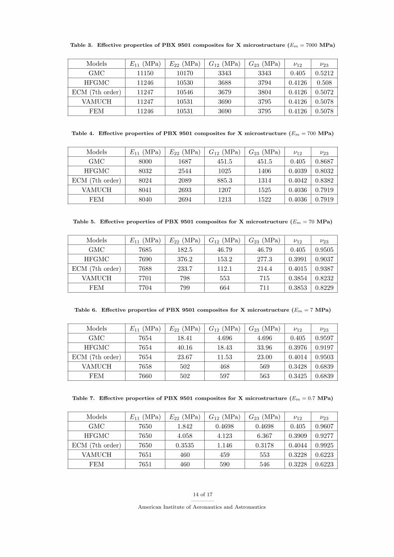
Table 3. Effective properties of PBX 9501 composites for X microstructure (Em = 7000 MPa)


GMC 11150 10170 3343 3343 0.405 0.5212HFGMC 11246 10530 3688 3794 0.4126 0.508


FEM 11246 10531 3690 3795 0.4126 0.5078



GMC 8000 1687 451.5 451.5 0.405 0.8687HFGMC 8032 2544 1025 1406 0.4039 0.8032

ECM (7th order) 8024 2089 885.3 1314 0.4042 0.8382VAMUCH 8041 2693 1207 1525 0.4036 0.7919

FEM 8040 2694 1213 1522 0.4036 0.7919



GMC 7685 182.5 46.79 46.79 0.405 0.9505HFGMC 7690 376.2 153.2 277.3 0.3991 0.9037

ECM (7th order) 7688 233.7 112.1 214.4 0.4015 0.9387VAMUCH 7701 798 553 715 0.3854 0.8232

FEM 7704 799 664 711 0.3853 0.8229



GMC 7654 18.41 4.696 4.696 0.405 0.9597HFGMC 7654 40.16 18.43 33.96 0.3976 0.9197


FEM 7660 502 597 563 0.3425 0.6839

Table 7. Effective properties of PBX 9501 composites for X microstructure (Em = 0.7 MPa)


GMC 7650 1.842 0.4698 0.4698 0.405 0.9607HFGMC 7650 4.058 4.123 6.367 0.3909 0.9277


FEM 7651 460 590 546 0.3228 0.6223

14 of 17


Em = 0.7 MPa, the predictions of ECM for E22 and G23 are the lowest, while the method predicts thehighest value for ν23.

At this stage, we believe it is premature to conclude which sets of predictions are more reliable thanothers. First of all, it is impractical to connect two fibers through one material point (the corner). It isa mathematical idealization of small contacting areas. The singularity due to the stress bridging throughthe connecting corners creates difficult for all numerical approaches. Second, we are limited by resourcesto perform convergence studies for FEM results because its calculations except G23 requires 3D analysis.Although one would tend to blindly believe that the FEM results are the most reliable, this is not necessarilytrue. The reason is that even if all the results are converged, we have strong reasons to believe the assumedboundary conditions, particularly those applied for transverse shear and longitudinal shear, will significantlyaffect the results because of the extreme microstructural construction and contrast ratio of constituentproperties.

Nevertheless, the aforementioned points by no means diminish the value of this case and the significanceof the presented results. Due to its special construction and high contrast ratio, this case provides a greatchallenge to all micromechanics approaches. It clearly discloses the fallacy about micromechanics thatevery model “works” as far as effective properties concerned. This is a case worthy of the attention ofthe micromechanics community and more extensive research on issues such as convergence studies, sizeeffects of the contacting areas, and even physical experiments, which are needed to make more authoritativeconclusions.

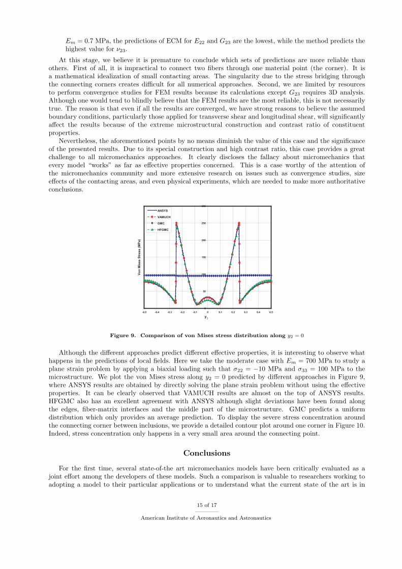
0

50

100

150

200

250

300

-0.5 -0.4 -0.3 -0.2 -0.1 0 0.1 0.2 0.3 0.4 0.5

Vo

n M

ise

s S

tres

s (

MP

a)

ANSYS

VAMUCH

GMC

HFGMC

y3

Figure 9. Comparison of von Mises stress distribution along y2 = 0

Although the different approaches predict different effective properties, it is interesting to observe whathappens in the predictions of local fields. Here we take the moderate case with Em = 700 MPa to study aplane strain problem by applying a biaxial loading such that σ22 = −10 MPa and σ33 = 100 MPa to themicrostructure. We plot the von Mises stress along y2 = 0 predicted by different approaches in Figure 9,where ANSYS results are obtained by directly solving the plane strain problem without using the effectiveproperties. It can be clearly observed that VAMUCH results are almost on the top of ANSYS results.HFGMC also has an excellent agreement with ANSYS although slight deviations have been found alongthe edges, fiber-matrix interfaces and the middle part of the microstructure. GMC predicts a uniformdistribution which only provides an average prediction. To display the severe stress concentration aroundthe connecting corner between inclusions, we provide a detailed contour plot around one corner in Figure 10.Indeed, stress concentration only happens in a very small area around the connecting point.

Conclusions

For the first time, several state-of-the art micromechanics models have been critically evaluated as ajoint effort among the developers of these models. Such a comparison is valuable to researchers working toadopting a model to their particular applications or to understand what the current state of the art is in

15 of 17


Figure 10. Contour plot of von Mises stress (MPa) distribution around a connecting corner

predictive capabilities in the field of micromechanics. Additionally the presented results (especially the localfield predictions) will represent test cases for researchers seeking to determine the accuracy of the predictivecapabilities of new micromechanics models. The X shape microstructure provides a very challenging testcase for all micromechanics approaches, and more research is needed to pinpoint the real limits of themicromechanics approach in general, and various micromechanics models in particular.

Acknowledgements

The first author and last author would like to acknowledge the support of the National Science Foundation.The second author would like to acknowledge the support of the Los Alamos National Laboratory and theASC program. The third and fourth authors would like to acknowledge the support of NASA Glenn ResearchCenter.

References

1Jones, R., Mechanics of Composite Materials, Hemisphere, New York, NY, 1975.2Herakovich, C., Mechanics of Fibrous Composites, John Wiley and Sons, New York, NY, 1998.3Mori, T. and Tanaka, K., “Average Stress in Matrix and Average Elastic Energy of Materials with Misfitting Inclusions,”

Acta Materialia, Vol. 21, 1973, pp. 571–574.4Benveniste, Y., “A New Approach to the Application of Mori-Tanaka’s Theory in Composite Materials,” Mechanics of

Materials, Vol. 36, 1987, pp. 147–157.5Williams, T. O., “A Generalized, Elasticity-based Theory for the Homogenization of Hetergeneous Materials with Complex

Microstructures,” 2007, in preparation.6Aboudi, J., Mechanics of Composite Materials: A Unified Micromechanics Approach, Elsevier, New York, NY, 1991.7Paley, M. and Aboudi, J., “Micromechanical Analysis of Composites by the Generalized Method of Cells,” Mechanics of

Materials, Vol. 14, 1992, pp. 127–139.8Aboudi, J., “Micromechanical Analysis of Thermo-Inelastic Multiphase Short-Fiber Composites,” Composites Engineer-

ing, Vol. 5, 1995, pp. 839–850.9Aboudi, J., “Micromechanical Analysis of Composites by the Method of Cells - Update,” Applied Mechanics Reviews,

Vol. 49, 1996, pp. 127–139.10Aboudi, J., “Micromechanical Analysis of Fully Coupled Electro-Magneto-Thermo-Elastic Multiphase Composites,”

Smart Materials and Structures, Vol. 10, 2001, pp. 867–877.11Williams, T. O., “A Two-dimensional, Higher-oder, Elasticity-based Micromechanics Model,” International Journal of

Solids and Structures, Vol. 42, 2005, pp. 1009–1038.12Williams, T. O., “A Three-dimensional, Higher-oder, Elasticity-based Micromechanics Model,” International Journal of

Solids and Structures, Vol. 42, 2005, pp. 971–1007.

16 of 17


13Nemat-Nasser, S. and Hori, M., Micromechanics: Overall Properties of Heterogeneous Materials, North-Holland, NewYork, NY, 1993.

14Bensoussan, A., Lions, J.-L., and Papanicolaou, G., Asymptotic Analysis for Periodic Structures, Elsevier, New York,NY, 1978.

15Yu, W., “A Variational-Asymptotic Cell Method for Periodically Heterogeneous Materials,” Proceedings of the 2005ASME International Mechanical Engineering Congress and Exposition, ASME, Orlando, Florida, Nov. 5–11 2005.

16Yu, W. and Tang, T., “Variational Asymptotic Method for Unit Cell Homogenization of Periodically HeterogeneousMaterials,” International Journal of Solids and Structures, Vol. 44, 2007, pp. 4039–4052.

17Yu, W. and Tang, T., “A New Micromechanics Model for Predicting Thermoelastic Properties of Heterogeneous Materi-als,” International Journal of Solids and Structures, 2007, submitted.

18Sun, C. and Vaidya, R., “Prediction of Composite Properties from a Representative Volume Element,” CompositesScience and Technology, Vol. 86, 1996, pp. 171–179.

19Brockenbrough, J., Suresh, S., and Wienecke, H., “Deformation of Metal-Matrix Composites with Continuous Fibers:Geometrical Effects of Fiber Distribution and Shape,” Acta. Metall. Mater., Vol. 39, 1991, pp. 735–752.

20Brydon, A. D., Bardenhagen, S. G., Miller, E. A., and Seidler, G. T., “Simulation of the Densification of Real Open-CelledFoam Microstructures,” Journal of the Mechanics and Physics of Solids, Vol. 53, 2005, pp. 2638–2660.

21Lissenden, C. and Herakovich, C., “Comparison of Micromechanical Models for Elastic Properties,” Space ’92, Proceedingsof the 3rd International Conference, Denver, CO, Vol. 2, 1992, pp. 1309–1322.

22Pindera, M.-J. and Bednarcyk, B., “An Efficient Implementation of the Generalized Method of Cells for Unidirectional,Multi-Phased Composites with Complex Microstructures,” Composites: Part B , Vol. 30, 1999, pp. 1009–1038.

23Bednarcyk, B. and Pindera, M. J., “Inlastic Response of a Woven Carbon/Copper Composite Part II: MicromechanicsModel,” Journal of Composite Materials, Vol. 34, 2000, pp. 299–331.

24Aboudi, J., Pindera, M.-J., and Arnold, S., “Higher-Order Theory for Periodic Multiphase Materials with InelasticPhases,” International Journal of Plasticity, Vol. 19, 2003, pp. 805–847.

25Aboudi, J., “Harmonic Waves in Composite Materials,” Wave Motion, Vol. 8, 1986, pp. 289–303.26Aboudi, J., “Transient Waves in Composite Materials,” Wave Motion, Vol. 9, 1987, pp. 141–156.27Aboudi, J., “Wave Propagation in Damaged Composite Materials,” International Journal of Solids and Structures,

Vol. 24, 1988, pp. 117–138.28Aboudi, J., Pindera, M.-J., and Arnold, S., “Higher-Order Theory for Functionally Graded Materials,” Composites: Part

B , Vol. 30, 1999, pp. 777–832.29Arnold, S., Bednarcyk, B., and Aboudi, J., “Comparison of the Computational Efficiency of the Original Versus Refor-

mulated High-Fidelity Generalized Method of Cells,” NASA TM 2004-213438 , 2004.30Aboudi, J., “The Generalized Method of Cells and High-Fidelity Generalized Method of Cells Micromechanical Models

- A Review,” Mechanics of Advanced Materials and Structures, Vol. 11, 2004, pp. 329–366.31Bednarcyk, B. and Arnold, S., “MAC/GMC 4.0 User’s Guide,,” NASA/TM-2002-212077 , 2002.32Guedes, J. and Kikuchi, N., “Preprocessing and Postprocessing for Materials Based on the Homogenization Method with

Adaptive Finite Element Method,” Computer Methods in Applied Mechanics and Engineering, Vol. 83, 1990, pp. 143–198.33Eshelby, J. D., “The Determination of the Elastic Field of an Ellipsoidal Inclusion, and Related Problems,” Proc. R. Soc.

London A, 1957, pp. 376–396.

17 of 17


a critical evaluation of the predictive capabilities of...

Documents