climate change causes and hydrologic predictive capabilities

Climate Change Causes and Hydrologic Predictive Capabilities

V.V. Srinivas Associate Professor

Department of Civil Engineering Indian Institute of Science, Bangalore

[email protected]

1

Overview of Presentation

Climate Change Causes

Effects of Climate Change Hydrologic Predictive Capabilities to Assess Impacts of Climate Change

on Future Water Resources

GCMs and Downscaling Methods Typical case studies

Gaps where more research needs to be focused

2

Weather & Climate

Weather Definition: Condition of the atmosphere at a particular place and time Time scale: Hours-to-days Spatial scale: Local to regional Climate Definition: Average pattern of weather over a period of time Time scale: Decadal-to-centuries and beyond Spatial scale: Regional to global Climate Change Variation in global and regional climates

3

(Source: PhysicalGeography.net)

Variation in the solar output/radiation Sun-spots (dark patches) (11-years cycle)

Cyclic variation in Earth's orbital characteristics and tilt - three Milankovitch cycles Change in the orbit shape

(circular↔elliptical) (100,000 years cycle)

Changes in orbital timing of perihelion and aphelion – (26,000 years cycle)

Changes in the tilt (obliquity) of the Earth's axis of rotation (41,000 year cycle; oscillates between 22.1 and 24.5 degrees)

Climate Change – Causes 4

Volcanic eruptions

Ejected SO2 gas reacts with water vapor in stratosphere to form a dense optically bright haze layer that reduces the atmospheric transmission of incoming solar radiation

Figure : Ash column generated by the eruption of Mount Pinatubo. (Source: U.S. Geological Survey).

Climate Change - Causes 5

Variation in Atmospheric GHG concentration Global warming due to absorption of longwave radiation emitted from the

Earth's surface

Sources of GHGs Burning of fossil fuels

Agriculture: livestock, agricultural soils, and rice production

Land use and Forestry - act as a source/sink Oceans: release/absorb CO2 depending on temperature

Climate Change - Causes

IPCC, 2007

Others: Hydrofluorocarbons, Perfluorocarbons and Sulfur hexafluoride

6

Climate Change - Causes

Most of the pre-anthropogenic (pre-1850) decadal-scale temperature variations was due to changes in solar radiation and volcanism – [Crowley 2000, Science]

Most of the warming in 20th-century is due to increase in GHG resulting from anthropogenic causes – [Crowley 2000, Science]

Basis: • Reconstructed Northern Hemisphere temperatures and climate forcing

over the past 1000 years • Indices of volcanism, Solar variability, Changes in GHGs and

Tropospheric aerosols

7

Figure: Reconstructed and observed CO2 records for the past 400,000 years

Ref: http://www.climate.gov

Lake Vostok (400,000 years ago to 2,500 years ago)

Law Dome Ice Core (from 2,000 years ago to 1960)

Mauna Loa Record (from 1960 to 2008)

Effects of Climate Change

Lake Vostok : The largest of Antarctica's almost 400 known subglacial lakes Law Dome, East Antarctica Mauna Loa: One of five volcanoes that form the Island of Hawaii in the U.S. Station ALOHA: Deep water (~4,800 m) location approximately 100 km north of the Hawaiian Island of Oahu

8

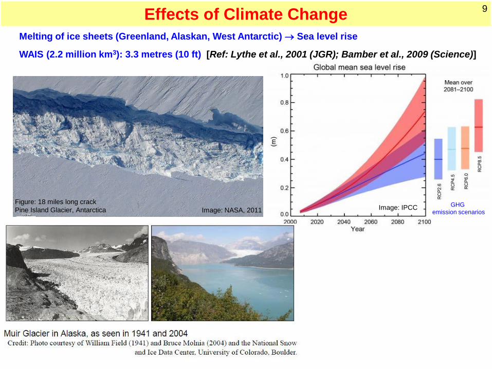
Melting of ice sheets (Greenland, Alaskan, West Antarctic) → Sea level rise

WAIS (2.2 million km3): 3.3 metres (10 ft) [Ref: Lythe et al., 2001 (JGR); Bamber et al., 2009 (Science)]

Image: NASA, 2011 Figure: 18 miles long crack Pine Island Glacier, Antarctica Image: IPCC GHG

emission scenarios

Effects of Climate Change 9

Changes to duration of seasons

Dieback of the Amazon rainforest (southern portion) due to increase in dry season length (by about a week per decade since 1979).

(Area: 1.4 billion acres, containing 90-140 billion metric tons of carbon) (could cause the release of large volumes of the CO2 into atmosphere) Changes to frequency and severity of hydrologic extremes such as floods

and droughts

Changes in the thermohaline circulation in the north Atlantic that affects global ocean heat transport

Intensification of desertification (through spatio-temporal variation in patterns of temperature, rainfall, solar radiation and winds) - West African Sahel, China

Effects of Climate Change 10

Hydrologic Predictive Capabilities to

Assess Impacts of Climate Change on Future Water Resources

http://www.teachengineering.org/

Water Balance

11

Ref: http://www.unep.org/dewa/vitalwater/article141.html

Future projections of water demand – Based on population growth

Future projections of water balance components – What can be the basis?

Hydrologic Predictive Capabilities 12

Simulate the response of the global climate system to future projections of

GHG emissions & Radiative forcing

General Circulation Models (GCMs) – Numerical Models

New Scenarios approved by IPCC in 2013

13

GCMs depict the climate using a three dimensional grid over the globe

Several vertical layers in the atmosphere and oceans

General Circulation Models (GCMs) 14

Climate model name

Agency/Source Atmospheric resolution

Oceanic resolution

BCC-CM1 Beijing Climate Center, China T63L16 1.875° x 1.875°, L30

BCCR: BCM2.0 Bjerknes Centre for Climate Research, Norway

T63L31 1.5° x (0.5°-1.5°), L35*

CCCma: CGCM3

Canadian Center for Climate Modelling and Analysis, Canada

T47, L31 1.8° x 1.8°, L29

T63, L31 1.4° Lon x 0.9° Lat, L29

CNRM-CM3 Centre National de Recherches Meteorologiques, France

T63, L45 182 x 152 grid†

CSIRO: MK3 Australia's Commonwealth Scientific and Industrial Research Organisation, Australia

T63, L18 1.875° Lon x approx. 0.84° Lat, L31

MPIM: ECHAM5-OM

Max-Planck-Institut for Meteorology, Germany

T63 L31 1.5°x1.5°, L40

T refers to horizontal resolution (number of waves with triangle truncation in horizontal direction) L refers to the number of vertical levels or layers.

General Circulation Models (GCMs) – Typical Examples 15

16

Simulate coarse-scale atmospheric dynamics reasonably well

Fail to simulate climate variables at finer watershed scale, as many of the physical processes which control local climate, e.g. topography, vegetation and hydrology, are not considered

General Circulation Models (GCMs) – Issues

Water Balance

Spatial Downscaling Dynamical downscaling Statistical downscaling Temporal downscaling/disaggregation

16

Dynamic downscaling Involves nesting of Regional Climate Model (RCM) in GCM Grid spacing of RCM: 20–50 km

Spatial Downscaling Methods – An Overview

GCM grid GCM grid

RCM grid

Target Region

RCM Accounts for finer-scale atmospheric dynamics (e.g., orographic precipitation) time-dependent lateral meteorological conditions defined by GCM

17

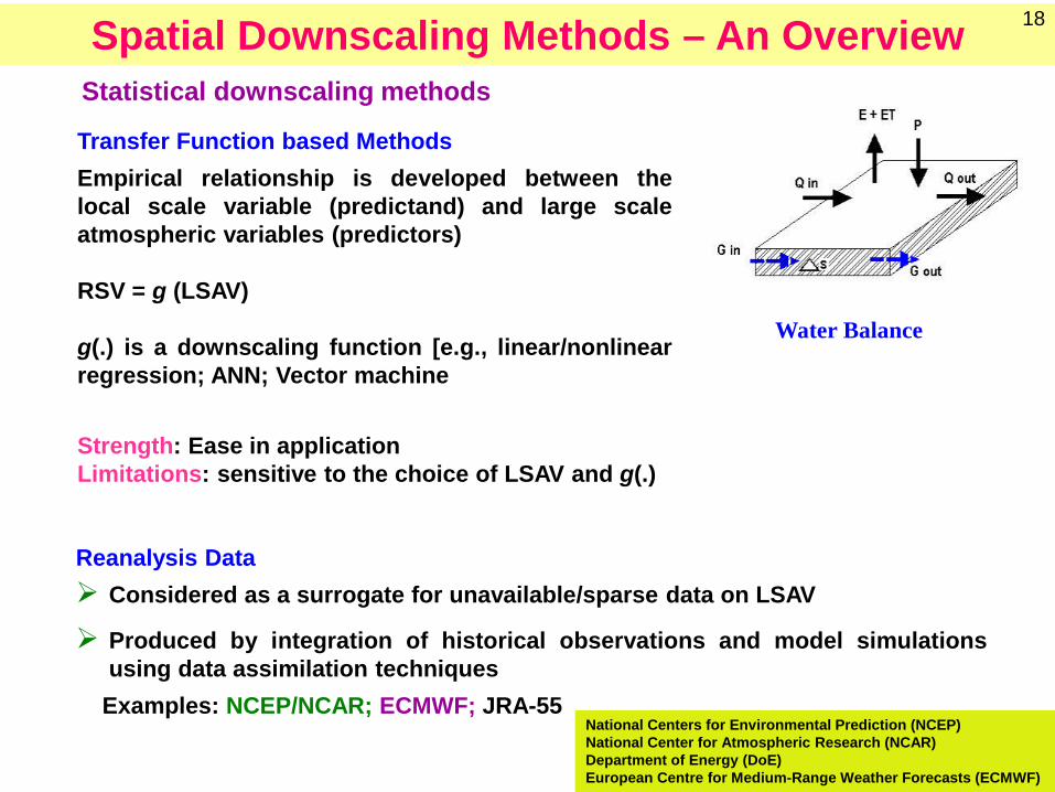
Statistical downscaling methods

Transfer Function based Methods Empirical relationship is developed between the local scale variable (predictand) and large scale atmospheric variables (predictors) RSV = g (LSAV)

g(.) is a downscaling function [e.g., linear/nonlinear regression; ANN; Vector machine

Strength: Ease in application Limitations: sensitive to the choice of LSAV and g(.)

Spatial Downscaling Methods – An Overview 18

Reanalysis Data Considered as a surrogate for unavailable/sparse data on LSAV

Produced by integration of historical observations and model simulations using data assimilation techniques

Examples: NCEP/NCAR; ECMWF; JRA-55 National Centers for Environmental Prediction (NCEP) National Center for Atmospheric Research (NCAR) Department of Energy (DoE) European Centre for Medium-Range Weather Forecasts (ECMWF)

Water Balance

Weather Typing Methods Local meteorological (predictand) data are partitioned into groups/clusters

based on past patterns of atmospheric circulation Future local climate scenarios are constructed by resampling predictand

data from clusters by conditioning on the future circulation patterns produced by a GCM

Limitation • Assume validity of the model parameters under future climate conditions

Stochastic Weather Generators

Climate change scenarios are generated stochastically using conventional weather generators by modifying their parameters conditional on outputs from a GCM

Examples: WGEN, LARS–WG or EARWIG

Limitation • Low skill at reproducing inter-annual to decadal climate variability • Unanticipated effects that changes to precipitation occurrence may have on

secondary variables such as temperature

Spatial Downscaling Models – An Overview 19

Predictors for downscaling different hydrometeorological variables

S N Predictors (coarser scale variables)

Predictand (local scale variable)

1

Temperature, geo-potential height, specific humidity, zonal and meridional wind velocities, precipitable water, surface pressure

Precipitation

2 Temperature at higher elevations

zonal and meridional wind velocities at higher elevations

Latent heat, sensible heat, shortwave radiation and longwave radiation fluxes

Max. & Min. temperature

3 zonal and meridional wind velocities at higher elevations Wind speed

4 Temperature at higher elevation Specific humidity at higher elevation Surface temperature, Latent heat flux

Relative humidity

5 Precipitable water Cloud cover

6 Mostly predictors selected for precipitation Some times wind speed, relative humidity, cloud cover

Streamflow

Predictor set depends on governing physical processes

Spatial Downscaling Models – An Overview 20

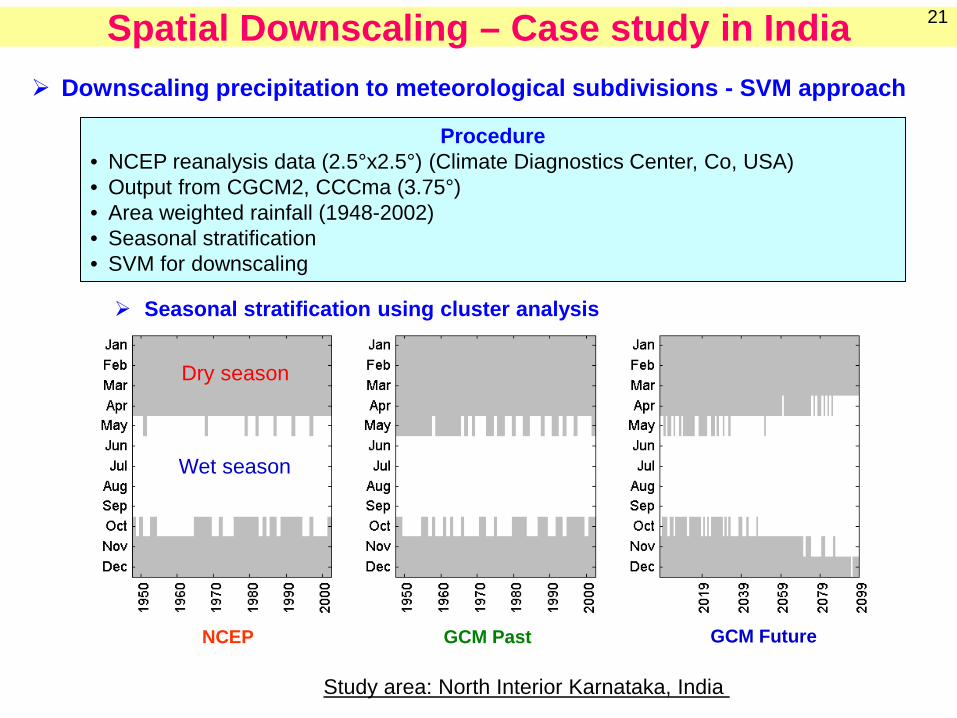
Downscaling precipitation to meteorological subdivisions - SVM approach

Procedure • NCEP reanalysis data (2.5°x2.5°) (Climate Diagnostics Center, Co, USA) • Output from CGCM2, CCCma (3.75°) • Area weighted rainfall (1948-2002) • Seasonal stratification • SVM for downscaling

Spatial Downscaling – Case study in India 21

NCEP GCM Past GCM Future

Seasonal stratification using cluster analysis

Dry season

Wet season

Study area: North Interior Karnataka, India

Results Significant increase in precipitation is projected for Konkan and Goa, Coastal Karnataka, Gujarat, Saurashtra and Kutch along west coast of India, Coastal Andhra Pradesh along east coast, Telangana and Rayalaseema in peninsula India, Punjab and Haryana in the north-west, east Uttar Pradesh, west Uttar Pradesh plains and Bihar plains in the north, and north Assam and south Assam in the north-east India. Drop in precipitation is projected for Kerala and East Madhya Pradesh, while mixed trend in precipitation is projected for the remaining parts of the country by the LS-SVM downscaling model for the simulations of CGCM2 model under IS92a scenario.

Ref: Tripathi et al. (2006) Published in J. of Hydrology

Spatial Downscaling – Case Study in India 22

Methods GCM simulated future streamflows are accepted

GCM simulated meteorological variables are used to drive a

hydrological model (unrealistic streamflows owing to inadequate and simplistic representation of the hydrologic cycle within GCMs) GCM simulated meteorological variables are downscaled to local scale

meteorological variables that are used to drive a hydrological model

GCM simulated LSAVs are downscaled to streamflow (Do not take into account dynamics of regional hydrological processes and the mechanisms governing streamflow generation in a watershed) Hydrological models are driven by hypothetical/synthetic or analogue

scenarios of meteorological variables

Future Streamflow projection in Climate Change Scenario 23

• Annual rainfall - 1051 mm • Catchment area: 2564 km2

• Gross storage capacity of dam: 1056 Mm3 (37.73 tmc)

Figure: NCEP & GCM grid points and rain gauge locations in Malaprabha reservoir catchment

Impact Assessment of Climate Change on Streamflows in Malaprabha Catchment


Ref: http://waterresources.kar.nic.in/salient_features_malaprabha.htm

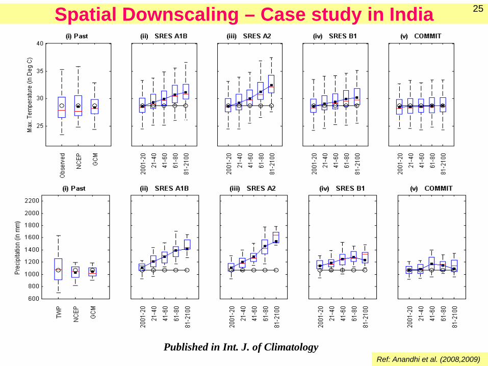
Precipitation

Published in Int. J. of Climatology Ref: Anandhi et al. (2008,2009)


Input for SWAT Model


Study area: Catchment of Malaprabha reservoir Calibration period: 1978-1993 Validation period: 1994 –2000

Bias in predicting peak flows is less for SWAT SBEM and DDSM under predicted high peaks and over predicted low peaks

SWAT : Soil and Water Assessment Tool SBEM : Support vector machine based empirical model DDSM : Direct downscaling model


ρ = 0.84

ρ = 0.98 ρ = 0.91

1mm: 2.564 Mm3

Figure: Projections for Monsoon Period (June-September)

The scenario A2 has the highest concentration of equivalent carbon dioxide (CO2) equal to 850 ppm, while the same for A1B, B1 and COMMIT scenarios are 720 ppm, 550 ppm and ≈ 370 ppm respectively.


What would be the implications of this uncertainty in river basin planning and management of water resources?

Monsoon streamflow∼ 950 Mm3 (Annual streamflow ∼ 1200 Mm3)

Multi-site downscaling of maximum and minimum daily temperature using support vector machine

Published in Int. J. of Climatology: 2014


Biases /change factors of the mean monthly climatology are computed

Strategy-1 Estimation of change between GCM past and station observations Application of bias corrections to GCM/RCM future simulations

Strategy-2 Estimation of change between GCM past and GCM future Application of bias correction to station observations Issue: The methods apply the correction to the mean and do not take account of model deficiencies in reproducing observed variability Strategy-3 Estimation of the percent changes in the climate variables per degree of

global warming for each season Scaling the values by three levels of global warming projected by IPCC

to obtain ‘‘seasonal scaling’’ factors Quantile-based strategies (Matching probability distributions of predictor variables in the GCM/RCM control simulations (1850-2000) to match probability distributions of observed predictor data

Bias correction / Change factor methodologies 30

Identification of appropriate predictors for downscaling in various parts of the world

Challenges: Understanding governing physical processes

Developing effective multi-site multivariate downscaling models

Challenges in modelling: Cross-correlations between time series of a predictand for all possible pairs of sites. Cross-correlations between time series of different predictands at each site and for all

possible pairs of sites

Developing methods to address uncertainty in choice of

Reanalysis data and spatial domain of predictors GCM and Climate change scenarios Method for re-gridding (GCM-to-Reanalysis) - Inverse square distance; bilinear ; Bessel Downscaling method Hydrological model: SWAT, HEC HMS, MIKE SHE, VIC, MODFLOW Relaxing assumption of stationarity in predictors -predictand relationship

Developing method to arrive at realistic future projections of extreme hydrologic events (floods and droughts)

Challenges: No proper strategy even in stationary scenario

Gaps where focused research is needed 31

Index flood procedure [Dalrymple, USGS, 1960]

ROI [Burn, 1990] & Regression Analysis [GLS, Stedinger & Tasker, 1985, USGS]

Gaps where focused research is needed 32

THANK YOU

climate change causes and hydrologic predictive capabilities

Documents